Optimizing the Age of Information in RIS-aided SWIPT Networks

Abstract

In this paper, a reconfigurable intelligent surface (RIS)-assisted simultaneous wireless information and power transfer (SWIPT) network is investigated. To quantify the freshness of the data packets at the information receiver, the age of information (AoI) is considered. To minimize the sum AoI of the information users while ensuring that the power transferred to energy harvesting users is greater than the demanded value, we formulate a scheduling scheme, and a joint transmit beamforming and phase shift optimization at the access point (AP) and RIS, respectively. The alternating optimization (AO) algorithm is proposed to handle the coupling between active beamforming and passive RIS phase shifts, and the successive convex approximation (SCA) algorithm is utilized to tackle the non-convexity of the formulated problems. The improvement in terms of AoI provided by the proposed algorithm and the trade-off between the age of information and energy harvesting is quantified by the numerical simulation results.

I Introduction

In beyond fifth generation (B5G) and sixth generation (6G) wireless network, challenging requirements are brought about by machine type communications (MTC) and the internet of things (IoT), which include massive connectivity, ultra reliability, low latency, as well as energy efficiency [1]. To realize self-sustainable communication systems in future wireless networks, the author in [18] first introduced the concept of simultaneous wireless information and power transfer (SWIPT) theoretically. Recently, SWIPT has becoming popular in the research of wireless communications [2].

To achieve the demands for ultra-reliable low latency communication (URLLC) with high quality of service (QoS), authors in [13] and [14] introduced a novel metric quantifying the freshness of information, namely the age of information (AoI) for the first times. The AoI is defined as the time elapsed since the generation of the last successfully delivered signal containing status update information about the system.In addition to traditional communication networks, the AoI has been considered in wireless powered networks [15, 16]. In [15], a wireless sensor network was studied with the sensor node which transmits status update packets harvesting energy from radio frequency signals, where the average AoI performance was analyzed and optimized with a greedy method. In [16], the authors investigated an age minimization problem in relay-aided two-hop energy harvesting networks.

Recently, reconfigurable intelligent surfaces (RIS) has emerged as a cost-efficient technology to compensate for the propagation attenuation and provide additional links for blocked direct links. Optimization on RIS aided networks have been investigated widely in the literature. In [7], the received power was maximized by jointly optimizing the transmit beamforming vectors and the phase shifts. Authors in [8] minimized the transmit power under the constraint of outage probability requirements. In [9], RIS was applied to SWIPT network to maximize the weighted sum power of energy harvesting receivers while guaranteeing signal-to-interference-plus-noise ratio (SINR) of information users. However, existing works of RIS mainly focused on the improvement of system capacity and energy efficiency. To the best of our knowledge, the investigation on information freshness improvement in RIS-aided SWIPT networks has not been studied yet.

Driven by this motivation, we study the sum AoI minimization in RIS-aided SWIPT networks. We construct a framework of RIS-assisted SWIPT network with multiple information receivers and energy receivers. An non-convex AoI optimization problem is formulated and solved by an successive convex approximation (SCA) based alternating optimization (AO) algorithm. Numerical results show the significant performance improvement of the proposed algorithm compared with maximum ratio transmission (MRT), random phase shifts case and active amplify-and-forward (AF) relay. Moreover, the trade-off between information freshness and energy harvesting is also highlighted in the simulation results.

II System Model and Problem Formulation

II-A Communication System Model

A RIS-aided wireless system is illustrated in Fig. 1, in which an access point (AP) configured with $N_{t}$ transmit antennas serves a SWIPT system with the assist of a RIS which has $N_{s}$ reflecting elements. We consider $U_{I}$ information streams at the AP forwarding status-update signals to the corresponding single-antenna information users (IUs), while $U_{E}$ energy streams are always forwarding energy packets to the single-antenna energy users (EUs), denoted by the sets $\mathcal{U_{I}}=\{1,...,U_{I}\}$ and $\mathcal{U_{E}}=\{1,...,U_{E}\}$, respectively. The time axis is measured by time slots indexed as $t\in\{1,2,...,T\}$. An update packet of information stream $i$ arrives at the system with probability $\lambda_{i}$ in each slot $t$. The indicator $a_{i}(t)\in\{0,1\}$ denotes whether the $i^{th}$ information stream has an arrived packet at AP or not.

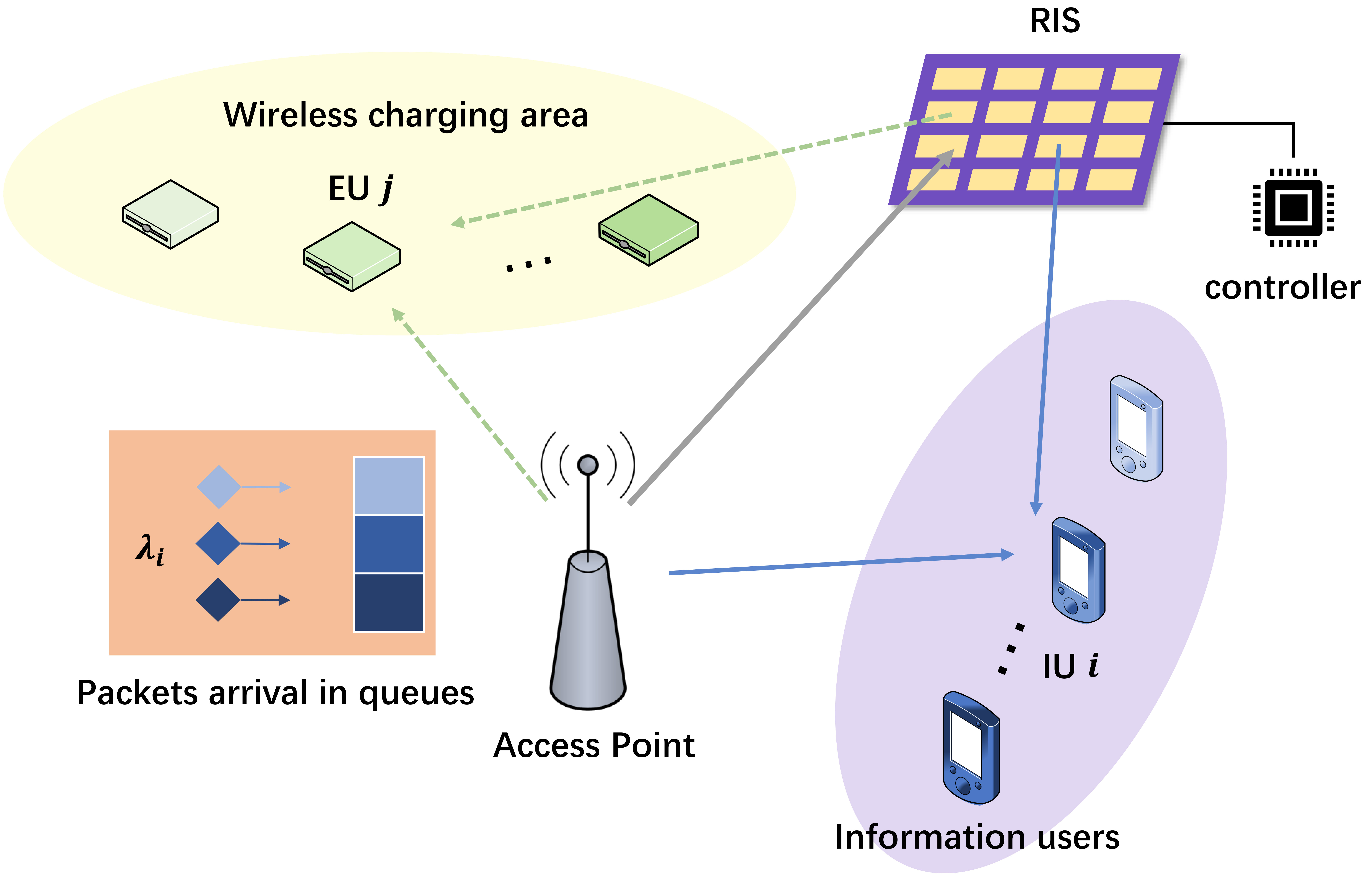
Figure 1: System model for the downlink SWIPT network.

Assume a time-varying flat fading channel model with coherent time lasting for one time slot. The channel state information (CSI) in each time slot is assumed to be perfectly known. Assume that the channels for each user are orthogonal without any interference, while the total scheduled information streams cannot exceed the total number of available information channels $M$. Therefore, a scheduling strategy is considered for information streams at the AP, which is constrained by

$$\sum_{i}\alpha_{i}(t)\leq M,$$ (1)

$$\alpha_{i}(t)\in\{0,1\},$$ (2)

where $\alpha_{i}(t)$ denotes the scheduling state at time slot $t$ for IU $i$.

The AP transmit signals separately to IU $i$ and the EU $j$ with $\bm{x}_{i}^{I}(t)=\bm{w}_{i}(t)s_{i}^{I}(t)$ and $\bm{x}_{j}^{E}(t)=\bm{v}_{j}(t)s_{j}^{E}(t)$, respectively, where $\bm{w}_{i}\in\mathbb{C}^{N_{t}\times 1}$ and $\bm{v}_{j}\in\mathbb{C}^{N_{t}\times 1}$ are the beamforming vectors for IU $i$ and EU $j$. Information and energy signals are denoted by $s_{i}^{I}(t)\sim\mathcal{CN}(0,1)$ and $s_{j}^{E}(t)\sim\mathcal{CN}(0,1)$, satisfying $\mathbb{E}(|s_{i}(t)|^{2})=1$ and $\mathbb{E}(|s_{j}(t)|^{2})=1$. The total transmit power is limited to be no more than $P_{0}$, such that

$$\sum_{i\in\mathcal{U_{I}}}||\bm{w}_{i}(t)||^{2}+\sum_{j\in\mathcal{U_{E}}}||\bm{v}_{j}(t)||^{2}\leq P_{0}{\color[rgb]{0,0,0}.}$$ (3)

The wireless transmission is assisted by the RIS, where $\bm{h}_{b,i}^{H}(t),\bm{h}_{r,i}^{H}(t),\bm{g}_{b,j}^{H}(t),\bm{g}_{r,j}^{H}(t)\in\mathbb{C}^{1\times N_{t}},\text{ and }\bm{G}(t)\in\mathbb{C}^{N_{s}\times N_{t}}$ denote the channels between AP and IU $i$, RIS and IU $i$, AP and EU $j$, RIS and EU $j$, AP and RIS, respectively. Define a reflection coefficient matrix $\bm{\Phi}(t)={\rm diag}(e^{j\theta_{1}(t)},e^{j\theta_{2}(t)},...,e^{j\theta_{N_{s}}(t)})\in\mathbb{C}^{N_{s}\times N_{s}}$, where $\theta_{n}$ is constrained by

$$\theta_{n}(t)\in[0,2\pi),\forall n\in\{1,2,...,N_{s}\},$$ (4)

which can be equivalently converted to a series of constraints of unit modulus

$$|e^{j\theta_{n}(t)}|=1,\forall n\in\{1,2,...,N_{s}\}.$$ (5)

The received SNR for IU $i$ is $\gamma_{i}(t)=\frac{|\bm{h}_{i}^{H}(t)\bm{w}_{i}(t)|^{2}}{\sigma_{i}^{2}}$, and the energy harvested by EU $j$ is $E_{j}(t)=|\bm{g}_{j}^{H}(t)\bm{v}_{j}(t)|^{2}$, where $\bm{h}_{i}^{H}(t)=\bm{h}_{r,i}^{H}(t)\bm{\Phi}(t)\bm{G}(t)+\bm{h}_{b,i}^{H}(t)$, and $\bm{g}_{j}^{H}(t)=\bm{g}_{r,j}^{H}(t)\bm{\Phi}(t)\bm{G}(t)+\bm{g}_{b,j}^{H}(t)$ are the equivalent channels for IU $i$ and EU $j$.

II-B The Age of Information

Following [4], the AoI for IU $i$ at time slot $t$ is denoted as $A_{i}(t)$, which is given by

$$A_{i}(t+1)=\alpha_{i}(t)k_{i}(t)z_{i}(t)+(1-\alpha_{i}(t))(1-k_{i}(t))A_{i}(t)+\\ (1-\alpha_{i}(t))k_{i}(t)A_{i}(t)+\alpha_{i}(t)(1-k_{i}(t))A_{i}(t)+1,$$ (6)

where $z_{i}(t)$ is the system time of the packet as follows,

$$z_{i}(t+1)=\left\{\begin{aligned} &0&if\,a_{i}(t+1)=1,\forall i,t\\ &z_{i}(t)+1&otherwise.\end{aligned}\right.$$ (7)

$k_{i}(t)\in\{0,1\}$ is $1$ when the scheduled stream $i$ has an available packet, and it turns to $0$ only if the $i^{th}$ stream is scheduled and successfully delivered without any newly arrived packet in this queue. A successful delivery is considered when the stream is scheduled and the received SNR is no less than the threshold value,

$$\gamma_{i}(t)\geq\alpha_{i}(t)k_{i}(t)\gamma_{th},\;\forall i\in\mathcal{U_{I}}.$$ (8)

II-C Problem Formulation

To minimize the total AoI for $U_{I}$ information streams, the active beamforming vectors and RIS phase shifts with scheduling schemes are jointly optimized. The optimization problem is proposed as follows,

$$\mathrm{(P1)}: \min_{\alpha_{i}(t),\bm{\Phi}(t),\atop\bm{w}_{i}(t),\bm{v}_{j}(t)}\sum_{t}\sum_{i\in\mathcal{U_{I}}}A_{i}(t)$$ (9)

$${\rm s.t.}\quad (\ref{chanConst}),(\ref{schedIndic}),(\ref{powConst}),(\ref{phaseModu}),(\ref{SNRconst}),$$

$$E_{j}(t)\geq Q,\forall j\in\mathcal{U_{E}},$$ (10)

where (10) aims to guarantee the amount of harvested energy. Due to the fact that the AoI will rise linearly without successful delivery, the problem of minimizing the sum AoI becomes maximizing AoI reduction in each time slot[5], which is the difference between the AoI and the system time in the current slot. Therefore, the optimization problem is converted to (P2) as

$$\mathrm{(P2)}: \max_{\alpha_{i}(t),\bm{\Phi}(t),\atop\bm{w}_{i}(t),\bm{v}_{j}(t)}\sum_{i\in\mathcal{U_{I}}}(A_{i}(t)-z_{i}(t))\alpha_{i}(t)k_{i}(t)$$ (11)

$${\rm s.t.}\quad (\ref{chanConst}),(\ref{schedIndic}),(\ref{powConst}),(\ref{phaseModu}),(\ref{SNRconst}),(\ref{EUconst}).$$

However, (P2) is difficult to solve due to the non-convexity of the constraints in QoS and harvested power for the EUs as well as the highly-coupled variables. To address this issue, an alternating optimization (AO) algorithm based on successive convex approximation (SCA) algorithm is proposed in the next section.

III AO-based Solutions

In this section, an AO-based algorithm solving this problem is presented by dealing with two subproblems.

III-A Problem Reformulation

First, the intractable constraint (2) is relaxed as $\alpha_{i}(t)\in[0,1]$. Then, to convert the problem into a more friendly form, define $\rho_{n}(t)=e^{j\theta_{n}(t)}$ satisfying $|\rho_{n}(t)|=1$, and $\bm{\rho}^{H}(t)=[\rho_{1}(t),\rho_{2}(t),...,\rho_{N_{s}}(t)]\in\mathbb{C}^{1\times N_{s}}$. Rewrite the equivalent channel for IU $i$ as $\bm{h}_{i}^{H}(t)=\bm{\rho}^{H}(t)\bm{U}_{i}(t)+\bm{h}_{b,i}^{H}(t)$, where $\bm{U}_{i}(t)={\rm diag}\Big{(}\bm{h}_{r,i}^{H}(t)\Big{)}\bm{G}(t)$. Similarly, the equivalent channel for EU $j$ is rewritten as $\bm{g}_{j}^{H}(t)=\bm{\rho}^{H}(t)\bm{V}_{j}(t)+\bm{g}_{b,j}^{H}(t)$. Thus, the problem is rewritten as

$$\mathrm{(P3)}:\max_{\alpha_{i}(t),\bm{\rho}(t),\atop\bm{w}_{i}(t),\bm{v}_{j}(t)}\sum_{i\in\mathcal{U_{I}}}(A_{i}(t)-z_{i}(t))\alpha_{i}(t)k_{i}(t)$$ (12)

$${\rm s.t.}\quad(\ref{chanConst}),(\ref{powConst}),$$

$$\quad\alpha_{i}(t)\in[0,1],$$ (12a)

$$\quad\big{|}\rho_{n}(t)\big{|}=1,\forall n\in\{1,2,...,N_{s}\},$$ (12b)

$$\quad\big{|}(\bm{\rho}^{H}(t)\bm{U}_{i}(t)+\bm{h}_{b,i}^{H}(t))\bm{w}_{i}(t)\big{|}^{2}\geq\alpha_{i}(t)k_{i}(t)\gamma_{th}\sigma_{i}^{2}{\color[rgb]{0,0,0},}$$ (12c)

$$\quad\big{|}(\bm{\rho}^{H}(t)\bm{V}_{j}(t)+\bm{g}_{b,j}^{H}(t))\bm{v}_{j}(t)\big{|}^{2}\geq Q{\color[rgb]{0,0,0}.}$$ (12d)

III-B Optimizing the Scheduling Policy and RIS Phase Shifts

To decompose the highly-coupled problem, we first optimize passive beamforming $\bm{\rho}(t)$ and scheduling indicator $\alpha_{i}(t)$ with given fixed $\bm{w}_{i}(t)$ and $\bm{v}_{j}(t)$. We employ the penalty method to deal with the non-convexity of constraint (5) by introducing a large positive constant $C$, where (P3) is reformulated as

$$\mathrm{(P4)}: \max_{\alpha_{i}(t),\bm{\rho}(t)}\sum_{i\in\mathcal{U_{I}}}(A_{i}(t)-z_{i}(t))\alpha_{i}(t)k_{i}(t)+C\sum_{n=1}^{N_{s}}(|\rho_{n}(t)|^{2}-1)$$ (13)

$${\rm s.t.}\quad(\ref{chanConst}),(\ref{relaschedIndic}),(\ref{SNRconst1}),(\ref{EUconst1}),$$

$$\quad|\rho_{n}(t)|\leq 1,\forall n\in\{1,2,...,N_{s}\}{\color[rgb]{0,0,0}.}$$ (13a)

It is noteworthy that when $C$ starts at a sufficiently small value, a good starting point of $\rho_{n}(t)$ can be given even though the unit modulus constraints are not satisfied. Then, we increase $C$ iteratively. With the value of $C$ becoming sufficiently large, the penalty will enforce $|\rho_{n}(t)|=1$ to obtain the optimum value (13). However, the objective function becomes non-convex due to the penalty term. To address this issue, SCA algorithm is utilized, where the objective function (13) is approximated as the first order Taylor expansion ([12]):

$$\sum_{i\in\mathcal{U_{I}}} (A_{i}(t)-z_{i}(t))\alpha_{i}(t)k_{i}(t)+2C\sum_{n=1}^{N_{s}}\mathcal{R}e\Big{\{}\Big{(}\rho_{n}^{(i-1)}(t)\Big{)}^{*}\Big{(}\rho_{n}(t)$$

$$- \rho_{n}^{(i-1)}(t)\Big{)}\Big{\}}+C\sum_{n=1}^{N_{s}}(|\rho_{n}^{(i-1)}(t)|^{2}-1),$$ (14)

where the value in the $(i-1)^{th}$ iteration is denoted by the superscript $(i-1)$.

Also, non-convex constraints (12c) and (12d) can be solved by SCA algorithm, with (12c) being approximated by

$$2\mathcal{R}e\Big{\{}\bm{w}_{i}^{H}(t)\Big{(}\bm{\rho}^{(i-1)H}(t)\bm{U}_{i}(t)+\bm{h}_{b,i}^{H}(t)\Big{)}^{H}\Big{(}\bm{\rho}(t)-\bm{\rho}^{(i-1)}(t)\Big{)}^{H}$$

$$\bm{U}_{i}(t)\bm{w}_{i}(t)\Big{\}}+\Big{|}\Big{(}\bm{\rho}^{(i-1)H}(t)\bm{U}_{i}(t)+\bm{h}_{b,i}^{H}(t)\Big{)}\bm{w}_{i}(t)\Big{|}^{2}$$

$$\geq\alpha_{i}(t)k_{i}(t)\gamma_{th}\sigma_{i}^{2},$$ (15)

where the lower bound of the left hand side (LHS) of the inequality is approximated by the first Taylor expansion with respect to $\bm{\rho}(t)$. Similarly, (12c) can be estimated as

$$2\mathcal{R}e\Big{\{}\bm{v}_{j}^{H}(t)\Big{(}\bm{\rho}^{(i-1)H}(t)\bm{V}_{i}(t)+\bm{g}_{b,j}^{H}(t)\Big{)}^{H}\Big{(}\bm{\rho}(t)-\bm{\rho}^{(i-1)}(t)\Big{)}^{H}$$

$$\bm{V}_{i}(t)\bm{v}_{j}(t)\Big{\}}+\Big{|}\Big{(}\bm{\rho}^{(i-1)H}(t)\bm{V}_{j}(t)+\bm{g}_{b,j}^{H}(t)\Big{)}\bm{v}_{j}(t)\Big{|}^{2}$$

$$\geq Q,\vspace*{-0.5cm}$$ (16)

Accordingly, the non-convex problem (P4) is converted as

$$\mathrm{(P5)}: \max_{\alpha_{i}(t),\bm{\rho}(t)}\sum_{i\in\mathcal{U_{I}}}(A_{i}(t)-z_{i}(t))\alpha_{i}(t)k_{i}(t)$$

$$+2C\sum_{n=1}^{N_{s}}\mathcal{R}e\Big{\{}\Big{(}\rho_{n}^{(i-1)}(t)\Big{)}^{*}\Big{(}\rho_{n}(t)-\rho_{n}^{(i-1)}(t)\Big{)}\Big{\}},$$ (17)

$${\rm s.t.}\quad(\ref{chanConst}),(\ref{relaschedIndic}),(\ref{phaseModu2}),(\ref{TaySNRalg2}),(\ref{TayEUalg2}).$$

where the last term of (14) is omitted since it is a constant.

Algorithm 1 Scheduling Scheme and Phase Shifts Optimization

1:Initialize $\bm{\rho}^{(0)}(t),\alpha^{(0)}_{i}(t),\bm{w}_{i}(t),\bm{v}_{j}(t),\;\forall i\in\mathcal{U_{I}}$, $\forall j\in\mathcal{U_{E}}.$ Set iteration index $n=1$.

2:repeat

3:    Update $\alpha_{i}^{(n)}(t),\bm{\rho}^{(n)}(t)$ by solving problem (P5).

4:until Convergence.

5:Output $\bm{\rho}^{(n)}(t)$.

Therefore, (P5) becomes a convex problem that can be efficiently solved by standard optimization software such as CVX [10]. The pseudo code Algorithm 1 gives a summary of the SCA-based algorithm 1.

III-C Optimizing the Scheduling Scheme and Active Beamforming Design

Given the fixed phase shift $\bm{\rho}(t)$ obtained by the last sub-problem, we optimize $\bm{w}_{i}(t)$ and $\bm{v}_{j}(t)$ while updating $\alpha_{i}(t)$. Similarly, SCA algorithm is employed to handle the non-convexity in constraints (12c) and (12d), where constraint (12c) is approximated by the first Taylor expansion with respect to $\bm{w}_{i}(t)$,

$$2\mathcal{R}e\Big{\{}\bm{w}_{i}^{(i-1)H}(t)\bm{h}_{i}(t)\bm{h}_{i}^{H}(t)\Big{(}\bm{w}_{i}(t)-\bm{w}_{i}^{(i-1)}(t)\Big{)}\Big{\}}$$

$$+\big{|}\bm{h}_{i}^{H}(t)\bm{w}_{i}^{(i-1)}(t)\big{|}^{2}\geq\alpha_{i}(t)k_{i}(t)\gamma_{th}\sigma_{i}^{2},$$ (18)

where $(i-1)$ denotes the value in the $(i-1)^{th}$ iteration. (12d) can be rewritten as

$$2\mathcal{R}e\Big{\{}\bm{v}_{j}^{(i-1)H}(t)\bm{g}_{j}(t)\bm{g}_{j}^{H}(t)\Big{(}\bm{v}_{j}(t)-\bm{v}_{j}^{(i-1)}(t)\Big{)}\Big{\}}$$

$$+\big{|}\bm{g}_{j}^{H}(t)\bm{v}_{j}^{(i-1)}(t)\big{|}^{2}\geq Q(t).$$ (19)

Then, (P3) becomes

$$\mathrm{(P6)}: \max_{\alpha_{i}(t),\atop\bm{w}_{i}(t),\bm{v}_{j}(t)}\sum_{i\in\mathcal{U_{I}}}(A_{i}(t)-z_{i}(t))\alpha_{i}(t)k_{i}(t)$$ (20)

$${\rm s.t.}(\ref{chanConst}),(\ref{powConst}),(\ref{relaschedIndic}),(\ref{TaySNR}),(\ref{TayEU}),$$

which is a convex problem and CVX can be used to solve it [10]. Finally, a stationary point can be obtained by solving a series of approximated convex problems. The corresponding algorithm for scheduling and beamforming optimization is presented in the pseudo code Algorithm 2. As a result, through the alternating optimization between (P5) and (P6), the value of the objective function will eventually converge to a local optimum.

Algorithm 2 Scheduling and Beamforming Optimization

1:Initialize $\alpha_{i}^{(0)}(t),\bm{w}_{i}^{(0)}(t),\bm{v}_{j}^{(0)}(t),\bm{\rho}(t),\;\forall i\in\mathcal{U_{I}}$, $\forall j\in\mathcal{U_{E}}.$ Set iteration index $n=1$.

2:repeat

3:     Update $\alpha_{i}^{(n)}(t),\bm{w}_{i}^{(n)}(t),\bm{v}_{j}^{(n)}(t)$ by solving problem (P6).

4:until Convergence.

5:Output $\alpha_{i}^{(n)}(t),\bm{w}_{i}^{(n)}(t),\bm{v}_{j}^{(n)}(t)$.

III-D Complexity Analysis

The overall computational complexity is based on the two proposed algorithms. The passive optimization problem is solved by SCA based penalty method, whose complexity is $\mathcal{O}\Big{(}S_{1}TU_{I}^{3.5}\log_{2}(1/\epsilon_{1})\Big{)}$, where $S_{1}$ denotes the number of SCA iterations, $T$ denotes the number of iterations to increase $C$, $U_{I}^{3.5}$ is the complexity of interior-point method in CVX, and $\epsilon_{1}$ is the accuracy of the SCA algorithm. The complexity of Algorithm 2 is $\mathcal{O}\big{(}S_{2}N_{s}^{3.5}\log_{2}(1/\epsilon_{2})\big{)}$. Hence, the overall computational complexity of the proposed AO algorithm is $\mathcal{O}\Big{(}S_{A}(S_{1}TU_{I}^{3.5}\log_{2}(1/\epsilon_{1})+S_{2}N_{s}^{3.5}\log_{2}(1/\epsilon_{2}))\Big{)}$, where $S_{A}$ is the number of alternating iterations.

IV Numerical Results

To quantify the effectiveness of the proposed algorithm, we perform numerical simulations with $U_{I}=3$ information users and $U_{E}=3$ energy users, respectively. We assume $N_{t}=4$ transmit antennas at the AP, and single antenna receivers. The packet arriving probabilities $\lambda_{i}$ are all set as 0.6. The noise power is set to be $-70\ {\rm dBm}$. Besides, $M=2$ available information channels are supposed.

We consider Rayleigh fading channels with large scale attenuation, where the independent channels are given as

$$\bm{h}_{b,i}(t)=A_{b,i}\bar{\bm{h}}_{b,i}(t){\color[rgb]{0,0,0},}\;\bm{h}_{r,i}(t)=A_{r,i}\bar{\bm{h}}_{r,i}(t){\color[rgb]{0,0,0},}$$

$$\bm{g}_{b,j}(t)=A_{b,j}\bar{\bm{g}}_{b,j}(t){\color[rgb]{0,0,0},}\;\bm{g}_{r,j}(t)=A_{r,j}\bar{\bm{g}}_{r,j}(t){\color[rgb]{0,0,0},}$$

$$\bm{G}(t)=A_{G}\bar{\bm{G}}(t),$$ (21)

where $\bar{\bm{h}}_{b,i}(t)$, $\bar{\bm{h}}_{r,i}(t)$, $\bar{\bm{g}}_{b,j}(t)$, $\bar{\bm{g}}_{r,j}(t)$, $\bar{\bm{G}}(t)$ denote the Rayleigh fading channels of the 5 links. $A_{b,i}$, $A_{r,i}$, $A_{b,j}$, $A_{r,j}$, $A_{G}$ denote the corresponding large scale fading, which can be calculated as $A_{b,i}=\sqrt{A_{0}d_{b,i}^{-n_{b,i}}}$ (similar for other channels), where $A_{0}=-30\ {\rm dB}$ is the reference path loss at a distance $d_{0}=1\text{ m}$, and $n_{b,i}={n}_{b,j}=2.2$, $n_{r,i}=n_{r,j}=2.2$ and $n_{b,r}=3.5$ are the path loss exponents for AP-IU $i$ link, AP-EU $j$ link, RIS-IU $i$ link, RIS-EU $j$ link and AP -RIS link, respectively. The distances from the AP to the IUs and EUs are set to be $d_{b,i}=31\ \rm m$ and $d_{b,j}=3\ \rm m$, respectively. The AP-RIS distance is set as $d_{br}=3\ \rm m$ in Fig. 2(a) and Fig. 2(b).

In Fig. 2(a), the sum AoI increases with rising SNR threshold value $\gamma_{th}$, with the total transmit power set as $P_{0}=3\ \rm W$. The 3 solid lines shows the trade-off between the AoI and harvested energy of EUs. The sum AoI increases with growing energy harvesting threshold $Q$ from $-15\ {\rm dBm}$ to $-8\ {\rm dBm}$. Compared with conventional maximum ratio transmission (MRT) beamforming scheme, the proposed method shows significant AoI performance improvement with the same parameter configuration. In contrast, sum AoI is larger and grows faster with increasing SNR threshold using random phase shift even though $Ns$ is set to $200$. Moreover, the magenta dash line shows the sum AoI versus $\gamma_{th}$ in the case without EU receiver, from which we can see that sum AoI is lower than SWIPT case, because power allocation and passive beamforming can be adjusted to satisfy QoS of information receivers.

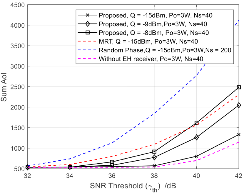
(a) Sum AoI versus SNR threshold $\gamma_{th}$.

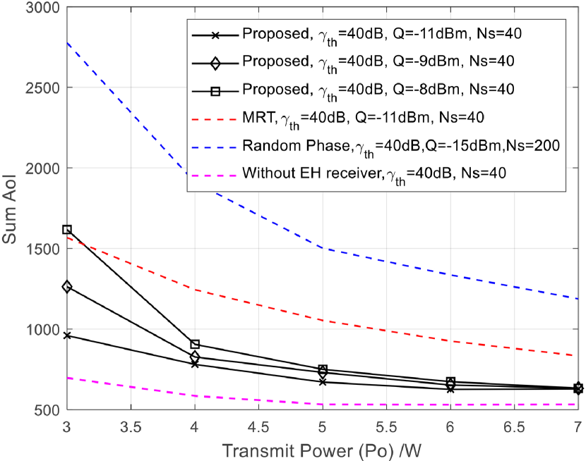
(b) Sum AoI versus transmit power $P_{0}$

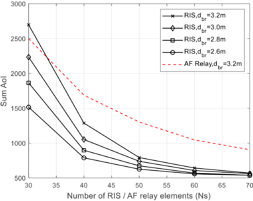
(c) Sum AoI versus the number of reflecting elements $N_{s}$

Figure 2: Simulation results

Fig. 2(b) demonstrates sum AoI reduction with growing transmit power. It is because larger transmit power enhances transmit signals, making the SNR and energy harvesting constraints to be more easily satisfied. Furthermore, the AoI and energy harvesting trade-off is also shown in Fig. 2(b), where more harvested energy results in worse performance on information freshness. Compared with MRT beamforming scheme and random phase scheme, the proposed AO algorithm shows drastic performance improvement. Compatible with the results in Fig. 2(a), without EH receiver case shows better AoI performance than SWIPT network.

In Fig. 2(c), we analyze how the number of RIS elements and the distance between the AP and the RIS effect the sum AoI, with $N_{s}$ increasing from 40 to 70. The 4 configurations are all set with $P_{0}=3\ \rm W,\gamma_{th}=40\ {\rm dB}\text{ and }Q=-10\ {\rm dBm}$, while the distance between the AP and the RIS changes between $3.2\ \rm m$ and $2.6\ \rm m$. It can be noticed that with growing number of reflecting elements, the AoI drops quickly to converge, showing the effectiveness of using RIS to enhance the wireless link. Moreover, the shorter distance from the AP to the RIS results in better AoI performance, because the channel gain is larger. In addition, AF relay is used instead of RIS. With the same power consumption, the sum AoI is lower than that of RIS-aided network at the beginning. However, with increasing elements, RIS outperforms AF relay. It is because RIS is passive without radio frequency (RF) chains, and thus RIS-aided networks consumes much lower power than AF relay with RF chains.

V Conclusion

We studied sum AoI optimization while satisfying the energy harvesting demands in a SWIPT network with the assistance of RIS. An SCA based AO algorithm was proposed to solve the scheduling problem with joint active and passive beamforming design. Numerical simulations showed the effectiveness of the proposed method compared with the conventional baselines, and trade-off between AoI and energy harvesting was illustrated by the numerical results.

[Proof of convergence of the proposed algorithms]

Algorithm 1 and Algorithm 2 are both based on SCA algorithm, where the convergence proof is similar. Thus, we take Algorithm 1 as an example, and convergence of Algorithm 2 can be proven as the same manner.

Recall that the problems (P4) and (P5) are equivalent. We show that (P5) can converge to a stationary point, which is equivalent to prove that of (P4). Based on constraints (12c) and (12d), we define the following functions

$$\mathcal{F}_{1}(\bm{\rho}(t),\alpha_{i}(t))=\alpha_{i}(t)k_{i}(t)\gamma_{th}\sigma_{i}^{2}-\big{|}(\bm{\rho}^{H}(t)\bm{U}_{i}(t)+\bm{h}_{b,i}^{H}(t))\bm{w}_{i}(t)\big{|}^{2},$$ (22)

$$\mathcal{F}_{2}(\bm{\rho}(t))=Q-\big{|}(\bm{\rho}^{H}(t)\bm{V}_{j}(t)+\bm{g}_{b,j}^{H}(t))\bm{v}_{j}(t)\big{|}^{2},$$ (23)

where $\mathcal{F}_{1}(\bm{\rho}(t),\alpha_{i}(t))\leq 0$ and $\mathcal{F}_{2}(\bm{\rho}(t))\leq 0$ are always guaranteed. With a series of transformations based on SCA algorithm, the above two functions are upper bounded by

$$\mathcal{\tilde{F}}_{1}(\bm{\rho}(t),\bm{\rho}^{(i-1)}(t),\alpha_{i}(t))=\alpha_{i}(t)k_{i}(t)\gamma_{th}\sigma_{i}^{2}$$

$$- 2\mathcal{R}e\Big{\{}\bm{w}_{i}^{H}(t)\Big{(}\bm{\rho}^{(i-1)H}(t)\bm{U}_{i}(t)+\bm{h}_{b,i}^{H}(t)\Big{)}^{H}\Big{(}\bm{\rho}(t)-\bm{\rho}^{(i-1)}(t)\Big{)}^{H}$$

$$\bm{U}_{i}(t)\bm{w}_{i}(t)\Big{\}}-\Big{|}\Big{(}\bm{\rho}^{(i-1)H}(t)\bm{U}_{i}(t)+\bm{h}_{b,i}^{H}(t)\Big{)}\bm{w}_{i}(t)\Big{|}^{2}$$ (24)

$$\mathcal{\tilde{F}}_{2}(\bm{\rho}(t),\bm{\rho}^{(i-1)}(t))=Q(t)$$

$$-2\mathcal{R}e\Big{\{}\bm{v}_{j}^{H}(t)\Big{(}\bm{\rho}^{(i-1)H}(t)\bm{V}_{i}(t)+\bm{g}_{b,j}^{H}(t)\Big{)}^{H}\Big{(}\bm{\rho}(t)-\bm{\rho}^{(i-1)}(t)\Big{)}^{H}$$

$$\bm{V}_{i}(t)\bm{v}_{j}(t)\Big{\}}-\Big{|}\Big{(}\bm{\rho}^{(i-1)H}(t)\bm{V}_{j}(t)+\bm{g}_{b,j}^{H}(t)\Big{)}\bm{v}_{j}(t)\Big{|}^{2},$$ (25)

which are differentiable. In proposed Algorithm 1, $\mathcal{F}_{1}(\bm{\rho}(t),\alpha_{i}(t))$ and $\mathcal{F}_{2}(\bm{\rho}(t))$ are replaced by $\mathcal{\tilde{F}}_{1}(\bm{\rho}(t),\bm{\rho}^{(i-1)}(t),\alpha_{i}(t))$ and $\mathcal{\tilde{F}}_{2}(\bm{\rho}(t),\bm{\rho}^{(i-1)}(t))$, respectively in each iteration of solving (P5). According to [17], the proposed SCA based Algorithm 1 converges to a Karush-Kuhn-Tucker (KKT) point of (P4) if the following conditions are satisfied:

$$\mathcal{F}_{1}(\bm{\rho}(t),\alpha_{i}(t))\leq\mathcal{\tilde{F}}_{1}(\bm{\rho}(t),\bm{\rho}^{(i-1)}(t),\alpha_{i}(t))$$ (26)

$$\mathcal{F}_{2}(\bm{\rho}(t))\leq\mathcal{\tilde{F}}_{2}(\bm{\rho}(t),\bm{\rho}^{(i-1)}(t)),$$ (27)

$$\frac{\partial\mathcal{F}_{1}(\bm{\rho}(t),\alpha_{i}(t))}{\partial\bm{\rho}(t)}=\frac{\partial\mathcal{\tilde{F}}_{1}(\bm{\rho}(t),\bm{\rho}^{(i-1)}(t),\alpha_{i}(t))}{\partial\bm{\rho}(t)},$$ (28)

$$\frac{\partial\mathcal{F}_{2}(\bm{\rho}(t))}{\partial\bm{\rho}(t)}=\frac{\partial\mathcal{\tilde{F}}_{2}(\bm{\rho}(t),\bm{\rho}^{(i-1)}(t))}{\partial\bm{\rho}(t)}.$$ (29)

Then, the above conditions can be verified by deriving the first-order derivatives of $\mathcal{F}_{1}(\bm{\rho}(t),\alpha_{i}(t))$, $\mathcal{F}_{1}(\bm{\rho}(t),\alpha_{i}(t))$, $\mathcal{F}_{2}(\bm{\rho}(t))$ and $\mathcal{\tilde{F}}_{2}(\bm{\rho}(t),\bm{\rho}^{(i-1)}(t))$ with respect to $\bm{\rho}(t)$. Notice that (p5) is equivalent to (P4), which means that Algorithm 1 can converge to a stationary KKT point of (P4). Moreover, the proof of convergence of Algorithm 2 can be similarly derived.

References

• [1] T. D. P. Perera, D. N. K. Jayakody, I. Pitas, and S. Garg, “Age of information in swipt-enabled wireless communication system for 5gb,” IEEE Wireless Commun., vol. 27, no. 5, pp. 162–167, 2020.
• [2] T. D. Ponnimbaduge Perera, D. N. K. Jayakody, S. K. Sharma, S. Chatzinotas, and J. Li, “Simultaneous wireless information and power transfer (swipt): Recent advances and future challenges,” IEEE Commun. Surv. Tutorials, vol. 20, no. 1, pp. 264–302, 2018.
• [3] L. R. Varshney, “Transporting information and energy simultaneously,” in 2008 IEEE International Symposium on Information Theory, 2008, pp. 1612–1616.
• [4] A. Muhammad, M. Elhattab, M. Shokry, and C. Assi, “Age of Information Optimization in a RIS-Assisted Wireless Network,” arXiv e-prints, p. arXiv:2103.06405, Mar. 2021.
• [5] S. Zhang, H. Zhang, Z. Han, H. V. Poor, and L. Song, “Age of information in a cellular internet of uavs: Sensing and communication trade-off design,” IEEE Trans. Wireless Commun., vol. 19, no. 10, pp. 6578–6592, 2020.
• [6] Q. Wu, S. Zhang, B. Zheng, C. You, and R. Zhang, “Intelligent reflecting surface-aided wireless communications: A tutorial,” IEEE Transactions on Communications, vol. 69, no. 5, pp. 3313–3351, 2021.
• [7] Q. Wu and R. Zhang, “Intelligent reflecting surface enhanced wireless network via joint active and passive beamforming,” IEEE Trans. Wireless Commun., vol. 18, no. 11, pp. 5394–5409, 2019.
• [8] G. Zhou, C. Pan, H. Ren, K. Wang, and A. Nallanathan, “Outage constrained transmission design for irs-aided communications with imperfect cascaded channels,” in GLOBECOM 2020 - 2020 IEEE Global Communications Conference, 2020, pp. 1–6.
• [9] Q. Wu and R. Zhang, “Weighted sum power maximization for intelligent reflecting surface aided swipt,” IEEE Wireless Commun. Letters, vol. 9, no. 5, pp. 586–590, 2020.
• [10] S. Boyd and L. Vandenberghe, Convex Optimization.   Cambridge university press, 2004.
• [11] C. Pan, H. Ren, K. Wang, J. F. Kolb, M. Elkashlan, M. Chen, M. Di Renzo, Y. Hao, J. Wang, A. L. Swindlehurst, X. You, and L. Hanzo, “Reconfigurable intelligent surfaces for 6g systems: Principles, applications, and research directions,” IEEE Commun. Mag., vol. 59, no. 6, pp. 14–20, 2021.
• [12] Z. Yang, M. Chen, W. Saad, W. Xu, M. Shikh-Bahaei, H. V. Poor, and S. Cui, “Energy-efficient wireless communications with distributed reconfigurable intelligent surfaces,” IEEE Trans. Wireless Commun., vol. 21, no. 1, pp. 665–679, 2022.
• [13] S. Kaul, R. Yates, and M. Gruteser, “Real-time status: How often should one update?” in 2012 Proceedings IEEE INFOCOM, 2012, pp. 2731–2735.
• [14] S. Kaul, M. Gruteser, V. Rai, and J. Kenney, “Minimizing age of information in vehicular networks,” in 2011 8th Annual IEEE Communications Society Conference on Sensor, Mesh and Ad Hoc Communications and Networks, 2011, pp. 350–358.
• [15] I. Krikidis, “Average age of information in wireless powered sensor networks,” IEEE Wireless Commun. Letters, vol. 8, no. 2, pp. 628–631, 2019.
• [16] A. Arafa and S. Ulukus, “Age-minimal transmission in energy harvesting two-hop networks,” in GLOBECOM 2017 - 2017 IEEE Global Communications Conference, 2017, pp. 1–6.
• [17] B. R. Marks and G. P. Wright, “A general inner approximation algorithm for nonconvex mathematical programs,” Operations Research, vol. 26, no. 4, pp. 681–683, 1978.
• [18] L. R. Varshney, “Transporting information and energy simultaneously,” in 2008 IEEE International Symposium on Information Theory, 2008, pp. 1612–1616.