Electroprewetting near a flat charged surface

Abstract

We look at the wetting of a pure fluid in contact with a charged flat surface. In the bulk, the fluid is a classical van der Waals fluid containing dissociated ions. The presence of wall and ions leads to strong dielectrophoretic and electrophoretic forces that increase the fluid’s density at the wall. We calculate the fluid’s profiles analytically and numerically and obtain the energy integrals. The critical surface potential for prewetting is obtained. In the phase diagrams, the line of first-order transition meets a second-order transition line at a critical point whose temperature can be higher or lower than the bulk critical temperature. The results are relevant to droplet nucleation around charged particles in the atmosphere and could possibly explain deviations from expected nucleation rates.

I Introduction

Fluids near or at charged surfaces are ubiquitous in every day life and in technology. The depth of penetration of the field into the fluid can vary from the molecular scale to infinity, in principle, depending on the fluids conductivity and on the geometry of electrodes producing the field. In the first edition of their book on electrodynamics of continuous media, Landau and Lifshitz calculated in a typical concise manner the change to the critical temperature $T_{c}$ [1]. Their reasoning was as follows: The electrostatic energy of perfect dielectrics is given by the integral $F_{\rm e}=-(1/2)\int\varepsilon_{0}\varepsilon(\phi){\bf E}^{2}{\rm d}^{3}r$, where ${\bf E}$ is the electric field, $\varepsilon_{0}$ is the vacuum permittivity, and $\varepsilon(\phi)$ is the relative dielectric constant, that depends on the scaled density (or composition, in the analogous case of binary mixtures), $\phi$. Close enough to the critical point, one can write $\varepsilon(\phi)$ as a Taylor-series expansion to quadratic order around $\phi_{c}$: $\varepsilon(\phi)\simeq\varepsilon_{c}+\Delta\varepsilon(\phi-\phi_{c})+(1/2)\varepsilon^{\prime\prime}(\phi-\phi_{c})^{2}$, where $\phi_{c}$ is the value of $\phi$ at the critical point, and $\varepsilon_{c}=\varepsilon(\phi_{c})$. When $\varepsilon(\phi)$ is multiplied by ${\bf E}^{2}$ in the electrostatic energy integral, and ${\bf E}$ is constant, the linear term in $\phi-\phi_{c}$ is simply a renormalization of the chemical potential. In a Landau expansion of the total energy in powers of $\phi-\phi_{c}$, the quadratic term in $F_{\rm e}$, proportional to $\varepsilon^{\prime\prime}$, simply renormalizes $T_{c}$, such that $T_{c}\to T_{c}+\Delta T$. For binary liquid mixtures, one obtains $\Delta T=v_{0}\varepsilon_{0}\varepsilon^{\prime\prime}E^{2}/k_{B}$, where $v_{0}$ is a molecular volume and $k_{B}$ is Boltzmann’s constant. Consequently, $T_{c}$ and the whole binodal curve are shifted upwards or downwards depending on the sign of $\varepsilon^{\prime\prime}$. For a pure liquid in coexistence with its vapor the behavior is similar. For values of $v_{0}$, $\varepsilon^{\prime\prime}$ and $E$ characteristic to experiments, one finds that $\Delta T$ is quite small, $\Delta T\sim 10$ mK.

The Landau prediction spurred several very accurate measurements of the shift to $T_{c}$, starting from P. Debye [2, 3, 4, 5, 6, 7]. But due to the smallness of the effect and some errors in several works, the problem gradually lost its allure.

Spatially nonuniform fields, on the other hand, have a much stronger effect on the phase behavior of fluids [8, 9]. When a spatially nonuniform field acts on a liquid mixture, if the field gradient is small, then the dielectrophoretic force “pulls” the more polar component toward the region where the field is high. If the external potential is small, then this effect is “obvious” in the sense that composition gradients are smooth. However, when the external potential is large enough, a sharp interface appears between two coexisting domains, one rich in the polar component and the other rich in the less polar liquid. The interface can appear far from a wall or at a surface, and the phase transition can be first or second order, depending on $T$, average composition $\phi_{0}$, and symmetry [10, 11, 12, 13]. The shift of the stability line separating the homogeneous and mixed states in field gradients is $10$–$100$ larger than in uniform fields (Landau).

In purely dielectric liquids (e.g., oils), the dielectrophoretic force is governed by the geometry of the electrodes producing the fields. In polar liquids on the other hand, dissociated ions are free to move. Their location is a balance among entropic, electrostatic, and chemical forces and it generally leads to screening of the field. Thus, field gradients occur irrespective of the electrode geometry. Importantly, when the ions move to the electrode they also “drag” the liquid in which they are better solvated, leading to a force of electrophoretic origin which is proportional to the preferential solvation.

The Gibbs transfer energy $\Delta G^{t}$ measures this preference and is sensitive to the ion and solvent combination. For example, for Na⁺ cations, $\Delta G^{t}=8.6$ kJ/mol for moving from water to methanol (Na⁺ “prefers” to be in water) but $\Delta G^{t}=-13.7$ kJ/mol for moving from water to dimethyl sulfoxide (it “prefers” to be in DMSO). The corresponding values for the hydrophilic Cl^- anion are both positive ($13.1$ and $39.4$ kJ/mol, respectively), and the values for the bulky hydrophobic anion sodium tetraphenylborate are $-24$ kJ/mol and $-37$ kJ/mol, respectively [14, 15]. Ion-specific effects play a central role in the solubility of proteins and leads to “salting out” [16], which is commonly used in protein separation techniques. Ionic specificity leads to the Hofmeister series [17, 18, 19, 20] and influences the air-water surface tension and the interaction between surface [21, 22, 23, 24, 25], [26].

In this paper, we study the coexistence of a vapor and liquid near a flat charged surface. The origin of field gradients is the presence of ions dissociated in the fluid. We look in details on the electroprewetting phenomenon, obtain the critical surface potential (or charge) for the phase transition, calculate the profiles, and show the resulting phase diagrams.

II Model

The starting point of the field-theoretic model is the free-energy integral

$$F = \int f{\rm d}{\bf r}+\int_{S}f_{\rm s}{\rm d}{\bf r}_{s},$$

where $f$ and $f_{s}$ are the bulk free energy and surface energy densities:

$$f = f_{\rm vdw}(T,\rho)+\frac{1}{2}c^{2}(\nabla\rho)^{2}+k_{B}T\left[n^{+}(\ln(v_{0}n^{+})-1)\right.$$

$$+ \left.n^{-}(\ln(v_{0}n^{-})-1)\right]-\frac{1}{2}\varepsilon_{0}\varepsilon(\rho)(\nabla\psi)^{2}$$

$$+ e(n^{+}-n^{-})\psi-k_{B}Tv_{0}(\Delta u^{+}n^{+}+\Delta u^{-}n^{-})\rho,$$

$$f_{\rm s} = v_{0}\rho\gamma_{\rm ls}+(1-v_{0}\rho)\gamma_{\rm gs}.$$ (1)

Here $\rho$ is the coarse-grained fluid’s density, $n^{\pm}$ are the cation and anion densities, $\varepsilon_{0}$ is the vacuum permittivity and $\varepsilon(\rho)$ is the relative dielectric constant, $\psi$ is the electrostatic potential, $k_{B}$ is the Boltzmann’s constant, $T$ is the absolute temperature, $v_{0}$ is a molecular volume (assumed the same for all molecules involved), $e$ is the unit charge, and $c$ is a constant. The surface integral is over the bounding surfaces; in this work we consider a semi-infinite system in the $x>0$ plane bounded by a single surface at $x=0$. The parameters $\gamma_{\rm ls}$ and $\gamma_{\rm gs}$ are the liquid-solid and gas-solid interfacial energies, respectively. The parameters $\Delta u^{\pm}$ measure the preferential solubility of the ions in the liquid. When they are positive, ions are attracted to the liquid phase, where $\rho$ is high. The derivation below is general for a bistable fluid, but for numerical purposes we will consider specifically the classical van der Waals fluid where $f_{\rm vdw}$ is given by

$$f_{\rm vdw}=k_{B}T\rho\left[\ln(\rho\Lambda^{3})-1-\ln(1-\rho b)\right]-a\rho^{2}.$$ (2)

Here $a$ and $b$ are the van der Waals interaction and excluded volume parameters, and $\Lambda$ is the de Broglie wavelength. The bulk critical point of the classical van der Waals fluid is given by $T_{c}=8a/27k_{B}b$, $\rho_{c}=1/3b$, and $P_{c}=a/27b^{2}$.

We proceed by defining dimensionless quantities as follows: $\tilde{f}=f/P_{c}$, $\phi=\rho/\rho_{c}$, $t=T/T_{c}$, and $\tilde{n}^{\pm}=v_{0}n^{\pm}$, $\tilde{\psi}=e\psi/k_{B}T$. In addition, all lengths are scaled as $\tilde{{\bf r}}={\bf r}/\lambda_{D0}$, where $\lambda_{D0}$ is the “vacuum” Debye length given by

$$\lambda_{D0}^{2}=\frac{\varepsilon_{0}v_{0}k_{B}T}{2\tilde{n}_{0}e^{2}}$$ (3)

and $\tilde{n}_{0}=v_{0}n_{0}$ is the scaled bulk ion concentration, far away from any charged surface. Lastly, we define $\tilde{P}$, $M$, “vacuum” Bjerrum length $l_{B}$ and $\tilde{c}$ as

$$\tilde{P} = \frac{k_{B}T}{v_{0}P_{c}},~{}~{}~{}~{}~{}~{}M=\tilde{P}\frac{v_{0}}{l_{B}\lambda_{D0}^{2}},$$

$$l_{B} = \frac{e^{2}}{\varepsilon_{0}k_{B}T},~{}~{}~{}~{}~{}~{}\tilde{c}^{2}=\frac{c^{2}\rho_{c}^{2}}{P_{c}\lambda_{D0}^{2}}.$$ (4)

The dimensionless bulk energy integral is therefore

$$\frac{F_{b}}{\lambda_{D0}^{3}P_{c}} = \int\left(\tilde{f}_{\rm vdw}(\phi)+\frac{1}{2}\tilde{c}^{2}(\tilde{\nabla}\phi)^{2}\right.$$ (5)

$$+ \tilde{P}[\tilde{n}^{+}(\ln(\tilde{n}^{+})-1)+\tilde{n}^{-}(\ln(\tilde{n}^{-})-1)]$$

$$- \frac{1}{2}M\varepsilon(\phi)(\tilde{\nabla}\tilde{\psi})^{2}+\tilde{P}(\tilde{n}^{+}-\tilde{n}^{-})\tilde{\psi}$$

$$- \left.\tilde{P}v_{0}\rho_{c}(\Delta u^{+}\tilde{n}^{+}+\Delta u^{-}\tilde{n}^{-})\phi\right){\rm d}\tilde{{\bf r}},$$

with

$$\tilde{f}_{\rm vdw}=(8t/3)\phi\left[\ln(\rho_{c}\phi\Lambda^{3})-1-\ln(1-\phi/3)\right]-3\phi^{2}.$$ (6)

For the surface energy, we repeat similar steps and obtain

$$\frac{F_{s}}{\lambda_{D0}^{3}P_{c}} = \int\Delta\tilde{\gamma}\phi d\tilde{{\bf r}}_{s}+{\rm const}$$ (7)

$$\Delta\tilde{\gamma} = \frac{v_{0}\rho_{c}(\gamma_{\rm ls}-\gamma_{\rm gs})}{\lambda_{D0}P_{c}}.$$

In equilibrium, the total free energy $F_{b}+F_{s}$ is at a minimum, and thus we look at the Euler-Lagrange equations for $\tilde{\omega}=\tilde{f}-\mu\phi-\mu^{+}\tilde{n}^{+}-\mu^{-}\tilde{n}^{-}$ with respect to the four fields $\phi$, $\tilde{n}^{\pm}$, and $\psi$:

$$\frac{\delta\tilde{\omega}}{\delta\phi} = \tilde{f}^{\prime}_{\rm vdw}(\phi)-\tilde{c}^{2}\tilde{\nabla}^{2}\phi-\frac{1}{2}M\frac{d\varepsilon}{d\phi}(\tilde{\nabla}\tilde{\psi})^{2}$$ (8)

$$- \tilde{P}v_{0}\rho_{c}(\Delta u^{+}\tilde{n}^{+}+\Delta u^{-}\tilde{n}^{-})-\mu=0,$$

$$\frac{\delta\tilde{\omega}}{\delta n^{\pm}} = \tilde{P}[\ln(\tilde{n}^{\pm})\pm\tilde{\psi}-v_{0}\rho_{c}\Delta u^{\pm}\phi]-\mu^{\pm}=0,$$ (9)

$$\frac{\delta\tilde{\omega}}{\delta\psi} = M\tilde{\nabla}[\varepsilon(\phi)\tilde{\nabla}\tilde{\psi}]+\tilde{P}(\tilde{n}^{+}-\tilde{n}^{-})=0.$$ (10)

$\mu$, $\mu^{+}$ and $\mu^{-}$ are the chemical potentials of the fluid density and the cation and anion densities, respectively. Equation (10) is the Poisson’s equation.

For a fluids in contact with a wall at scaled potential $\tilde{V}$ and bulk composition $\phi_{0}$, the boundary conditions are

$$\tilde{c}^{2}\phi^{\prime}(0) = \Delta\tilde{\gamma},~{}~{}~{}\phi(\infty)=\phi_{0}$$

$$\tilde{\psi}(0) = \tilde{V},~{}~{}~{}~{}~{}\tilde{\psi}(\infty)=0.$$

In the grand-canonical ensemble, the chemical potential is $\mu=\mu_{0}$ with

$$\mu_{0} = \tilde{f}^{\prime}_{\rm vdw}(\phi_{0})-2\tilde{P}\tilde{n}_{0}v_{0}\rho_{c}\Delta u.$$ (11)

We continue by focusing on the simple case where the two ions are equally “philic” to the liquid phase: $\Delta u^{\pm}=\Delta u$. We use $\varepsilon_{1}\approx 1$ and $\varepsilon_{2}$ as the permittivities of the vapor and pure liquid, respectively, and assume a dielectric constitutive relation of the form

$$\varepsilon(\phi)=\varepsilon_{1}+\Delta\tilde{\varepsilon}\phi+\frac{1}{2}\varepsilon^{\prime\prime}\phi^{2}.$$ (12)

To show a clear difference from the Landau mechanism, in most places below we will assume a linear relation with $\varepsilon^{\prime\prime}=0$ and $\Delta\varepsilon=(\varepsilon_{2}-\varepsilon_{1})/3$.

Far away from any charged surface, in the bulk reservoir, the electric potential vanishes, $\phi=\phi_{0}$ is a composition smaller than the lower binodal value, and $\tilde{n}=\tilde{n}_{0}$, hence the Euler-Lagrange equation for the ions is readily solved to yield the Boltzmann weight

$$\tilde{n}^{\pm}=\tilde{n}_{0}e^{\mp\tilde{\psi}+v_{0}\rho_{c}\Delta u(\phi-\phi_{0})}.$$ (13)

III Results

III.1 Critical value of the potential

The dielectrophoretic and electrophoretic forces in Eq. (8) lead to an increase of the fluid’s density near the wall. This increase is reminiscent of the increase in density of a fluid under the influence of gravity near the surface of Earth (though the electric field case is far richer because the fluid’s density changes the field, via the Poisson’s equation, a “back action” that is not present in the coupling between gravity and mass density) [27].

Because the fluid is bistable, if the surface potential is large enough, then a transition will occur from a gas to a liquid phase. To obtain the threshold value we substitute $\tilde{n}^{+}+\tilde{n}^{-}=2\tilde{n}_{0}e^{v_{0}\rho_{c}\Delta u(\phi-\phi_{0})}\cosh(\tilde{\psi})$ in Eq. (8) and obtain

$$\tilde{f}^{\prime}_{\rm vdw}(\phi) - \tilde{c}^{2}\tilde{\nabla}^{2}\phi-\frac{1}{2}M\Delta\varepsilon(\tilde{\nabla}\tilde{\psi})^{2}$$

$$- 2\tilde{P}\tilde{n}_{0}v_{0}\rho_{c}\Delta ue^{v_{0}\rho_{c}\Delta u(\phi-\phi_{0})}\cosh(\tilde{\psi})-\mu_{0}=0.$$

When $\varepsilon_{1}=\varepsilon_{2}$, the solution to the Poisson-Boltzmann problem [Eqs. (9)–(10)] is the classical nonlinear potential near a single wall:

$$\tilde{\psi}_{0} = 2\ln\left[\frac{1+Ce^{-\tilde{x}}}{1-Ce^{-\tilde{x}}}\right],~{}~{}~{}~{}~{}~{}C=\frac{e^{\tilde{V}/2}-1}{e^{\tilde{V}/2}+1}.$$ (15)

When $\varepsilon_{1}\neq\varepsilon_{2}$ and $\Delta\varepsilon$ is much smaller than the average dielectric constant $\bar{\varepsilon}$, the solution to the potential is $\tilde{\psi}=\tilde{\psi}_{0}+\tilde{\psi}_{1}$, where $\tilde{\psi}_{1}$ is of order $\Delta\varepsilon/\bar{\varepsilon}$. The field squared $(\tilde{\nabla}\tilde{\psi})^{2}$ in Eq. (III.1) can be expanded similarly in orders of $\Delta\varepsilon/\bar{\varepsilon}$. It is instructive to examine this equation to zero order in $\Delta\varepsilon/\bar{\varepsilon}$ and in the absence of preferential solvation ($\Delta u=0$); corrections will be the result of a loop expansion in higher orders in $\Delta\varepsilon/\bar{\varepsilon}$.

Cahn’s classical wetting construction cannot be performed here due to the existence of the long-range force [28, 29], but graphical solution of the equation for $\phi$ may be useful in the sharp interface limit ($\tilde{c}=0$), see Fig. 1. For simplicity, it is assumed here that $\varepsilon$ is linear in $\phi$ and that $\Delta u=0$. The black thin line is $\tilde{f}^{\prime}_{\rm vdw}(\phi)$ at a given temperature $t<1$. $\phi_{0}$ is the bulk composition and is assumed to be outside and on the left of the binodal curve. The solution to Eq. (III.1) is given graphically as an intersection between this curve and a nearly horizontal line $(1/2)M\Delta\varepsilon(\tilde{\nabla}\tilde{\psi})^{2}+\mu_{0}$. At $\tilde{x}=\infty$, the field is zero and $\tilde{f}^{\prime}_{\rm vdw}=\mu_{0}$ retrieves the bulk phase (red circle in the figure). As $\tilde{x}$ decreases, the field increases, the horizontal line sweeps upwards in Fig. 1, and the intersection moves to larger values of $\phi$. If the wall charge is not too large, then the locus of intersections is shown as a green solid line. The red diamond signifies the maximal value of $\phi$, obtained at the wall: $\phi_{s}=\phi(\tilde{x}=0)$. The resulting profile $\phi(\tilde{x})$ is smoothly decaying with $\tilde{x}$.

This behavior changes at large wall potentials. Let us denote by $\phi_{\rm s,l}$ and $\phi_{\rm s,h}$ the low and high spinodal compositions, respectively. $\phi_{\rm s,l}^{*}$ is the composition where $f^{\prime}_{\rm vdw}$ equals $f^{\prime}_{\rm vdw}(\phi_{\rm s,h})$. Similarly, $\phi_{\rm s,h}^{*}$ is the composition where $f^{\prime}_{\rm vdw}(\phi_{\rm s,h}^{*})=f^{\prime}_{\rm vdw}(\phi_{\rm s,l})$. Clearly, when the potential or charge increases sufficiently, the line $(1/2)M\Delta\varepsilon(\tilde{\nabla}\tilde{\psi})^{2}+\mu_{0}$ moves up so much that the solution to the equation is at large values of $\phi$. At these potentials, the profile is described by a “jump” from a low-$\phi$ part at large $\tilde{x}$ to a high-$\phi$ part at small $\tilde{x}$ . The compositions in both phases are not uniform. At the critical value for the transition, $\phi_{s}$ is larger than $\phi_{\rm s,l}^{*}$ and smaller than $\phi_{\rm s,l}$.

One can approximate the critical potential by assuming that the transition occurs at the lower binodal value, that is, when $\phi_{s}=\phi_{\rm b,l}$.

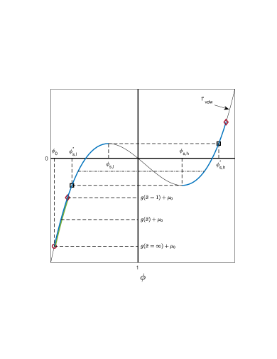
Figure 1: Graphical solution of Eq. (8) or Eq. (III.1) when $\varepsilon_{1}\approx\varepsilon_{2}$ and $\Delta u=0$. These equations can be written as $f^{\prime}_{\rm vdw}=g(\tilde{x})+\mu_{0}$, where $g(\tilde{x})=(1/2)M\Delta\varepsilon(\tilde{\nabla}\tilde{\psi})^{2}$ is a decreasing function of $\tilde{x}$. Curved black line is $f^{\prime}_{\rm vdw}$. The solution to the equation is the intersection between $f^{\prime}_{\rm vdw}$ and a nearly horizontal line. This line sweeps upwards as $\tilde{x}$ decreases from infinity, giving a smoothly decaying profile $\phi(\tilde{x})$ (green segment) when the surface potential $\tilde{V}$ is small. Red circle is the bulk composition and leftmost red diamond is the surface composition $\phi_{s}$. If $\tilde{V}$ is large enough, then coexistence between a vapor and a liquid is marked by a surface composition at large values of $\phi$ (rightmost red diamond).

Since $\left(4C/(C^{2}-1)\right)^{2}=2(\cosh(\tilde{V})-1)$, and in the sharp interface limit, this amounts to

$$\tilde{f}^{\prime}_{\rm vdw}(\phi_{\rm b,l})-M\Delta\varepsilon(\cosh(\tilde{V}_{c})-1)$$

$$-2\tilde{P}\tilde{n}_{0}v_{0}\rho_{c}\Delta ue^{v_{0}\rho_{c}\Delta u(\phi_{\rm b,l}-\phi_{0})}\cosh(\tilde{V}_{c})-\mu_{0}\approx 0,$$

or

$$\cosh(\tilde{V}_{c})\approx\frac{\tilde{f}^{\prime}_{\rm vdw}(\phi_{\rm b,l})-\mu_{0}+M\Delta\varepsilon}{M\Delta\varepsilon+2\tilde{P}\tilde{n}_{0}v_{0}\rho_{c}\Delta ue^{v_{0}\rho_{c}\Delta u(\phi_{\rm b,l}-\phi_{0})}}.$$

When $\tilde{V}\gg 1$, $\cosh(\tilde{V})-1\approx\cosh(\tilde{V})$ and we have

$$\cosh(\tilde{V}_{c})\approx\frac{\tilde{f}^{\prime}_{\rm vdw}(\phi_{\rm b,l})-\mu_{0}}{M\Delta\varepsilon+2\tilde{P}\tilde{n}_{0}v_{0}\rho_{c}\Delta ue^{v_{0}\rho_{c}\Delta u(\phi_{\rm b,l}-\phi_{0})}}.$$

In the opposite limit, $\tilde{V}_{c}\ll 1$, one obtains

$$\tilde{V}_{c}^{2}\approx\frac{\tilde{f}^{\prime}_{\rm vdw}(\phi_{\rm b,l})-2\tilde{P}\tilde{n}_{0}v_{0}\rho_{c}\Delta ue^{v_{0}\rho_{c}\Delta u(\phi_{\rm b,l}-\phi_{0})}-\mu_{0}}{\frac{1}{2}M\Delta\varepsilon+\tilde{P}\tilde{n}_{0}v_{0}\rho_{c}\Delta ue^{v_{0}\rho_{c}\Delta u(\phi_{\rm b,l}-\phi_{0})}}.$$

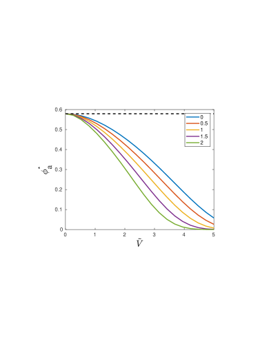
Figure 2: Plots of $\phi_{a}^{*}$, the value of the bulk composition $\phi_{0}$ obeying Eq. (III.1), as a function of surface potential $\tilde{V}$ and for a fixed reduced temperature $t=T/T_{c}=0.95$. The five curves correspond to the five values of $v_{0}\rho_{c}\Delta u$ indicated in the legend. Wetting of the surface occurs when $\phi_{0}>\phi_{a}^{*}$. Dashed horizontal line is the lower value of the binodal composition $\phi_{b,l}$ at the same temperature. The $\tilde{V}\ll 1$ and $\tilde{V}\gg 1$ limits are described by Eqs. (III.1) and (III.1), respectively. In this and in other figures (unless stated otherwise) we used $\tilde{n}_{0}=0.05$, $\varepsilon_{1}=1$, $\varepsilon_{2}=5$, and $\tilde{P}/t=0.4$.

The analytical equation Eq. (III.1) can be inverted to obtain the critical value of bulk composition $\phi_{a}^{*}$ for a given temperature and surface potential. Figure 2 shows $\phi_{a}^{*}$ vs $\tilde{V}$. When $\phi_{0}<\phi_{a}^{*}$, the profile $\phi(\tilde{x})$ is smoothly varying; when $\phi_{0}>\phi_{a}^{*}$, an electroprewetting transition occurs where a dense phase wets the surface in coexistence with a vapor phase away from it. At infinitesimal potential, Eq. (III.1) applies and $\phi_{a}^{*}$ is infinitesimally close to the lower binodal value $\phi_{b,l}$. As $\tilde{V}$ increases, $\phi_{a}^{*}$ decreases and the unstable “window” for electroprewetting $\phi_{b,l}-\phi_{a}^{*}$, widens. At large potentials Eq. (III.1) holds.

III.2 Phase diagrams

Before we evaluate the phase diagrams numerically let us continue with the sharp interface limit and examine the Euler-Lagrange equation for $\phi$ along with the second and third derivatives of the energy calculated at the surface:

$$f^{\prime}_{\rm vdw}(\phi_{s})-\frac{1}{2}M\frac{d\varepsilon}{d\phi}\psi_{s}^{\prime 2}$$

$$-2\tilde{P}\tilde{n}_{0}v_{0}\rho_{c}\Delta ue^{v_{0}\rho_{c}\Delta u(\phi_{s}-\phi_{0})}\cosh(\tilde{V})-\mu_{0} = 0~{},$$ (19)

$$f^{\prime\prime}_{\rm vdw}(\phi_{s})-\frac{1}{2}M\frac{d^{2}\varepsilon}{d\phi^{2}}\psi_{s}^{\prime 2}$$

$$-2\tilde{P}\tilde{n}_{0}(v_{0}\rho_{c}\Delta u)^{2}e^{v_{0}\rho_{c}\Delta u(\phi_{s}-\phi_{0})}\cosh(\tilde{V}) = 0~{},$$ (20)

$$f^{\prime\prime\prime}_{\rm vdw}(\phi_{s})-\frac{1}{2}M\frac{d^{3}\varepsilon}{d\phi^{3}}\psi_{s}^{\prime 2}$$

$$-2\tilde{P}\tilde{n}_{0}(v_{0}\rho_{c}\Delta u)^{3}e^{v_{0}\rho_{c}\Delta u(\phi_{s}-\phi_{0})}\cosh(\tilde{V}) = 0~{}.$$ (21)

where $-\psi_{s}^{\prime}$ is the value of the field at $\tilde{x}=0$. A simultaneous solution of Eqs. (19) and (20) yields $\phi_{0}(t)$ and $\phi_{s}(t)$ as two lines in the phase diagram. Simultaneous solution of Eqs. (19) and (21) yields another two lines $\phi_{0}(t)$ and $\phi_{s}(t)$. Figure 3 shows these lines for the case where $\varepsilon$ is a linear function of $\phi$ and with the approximation $\tilde{\psi}=\tilde{\psi}_{0}$ from Eq. (15). There are two solutions to Eqs. (19) and (20). The first is marked with circles (circles with line: $\phi_{0}$, circles only: $\phi_{s}$) and the second is marked with a plus “+” sign (“+” with line: $\phi_{0}$; “+” only: $\phi_{s}$). Black solid line is the bulk binodal curve. In part (a) the preferential solvation is zero ($\Delta u=0$) and $\phi_{s}$ are identical with the spinodal composition (dashed green line). Red solid curve is the solution for $\phi_{0}$ of Eqs. (19) and (21).

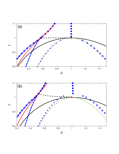
Figure 3: A solution of Eqs. (19) and (20) for the variables $\phi_{0}$ (bulk composition) and $\phi_{s}$ (surface composition) gives lines in the phase diagram (blue). These equations have two pairs of solutions – one is marked with circles [circles with line: $\phi_{0}(t)$; circles: $\phi_{s}(t)$] and one marked with “+” signs [“+” with line: $\phi_{0}(t)$; “+”: $\phi_{s}(t)$]. In (a) $v_{0}\rho_{c}\Delta u=0$ and $\phi_{s}(t)$ are identical with the bulk spinodal curves (dashed green line). In (b) $v_{0}\rho_{c}\Delta u=0.8$ and they are different. Red curve $\phi_{0}(t)$ is given from from Eqs. (19) and (21). This curve meets with the blue curves at a point marked with a square. In (a) this occurs at $t=1$ while in (b) it occurs at $t>1$. In both parts, the point marked with square is the simultaneous solution of Eqs. (19)–(21) for a given surface potential $\tilde{V}$ [in both (a) and (b) $\tilde{V}=2$]. The dashed line, obtained as the solution for $\tilde{V}$ diminishing to zero, is the approximation for the second-order phase transition line. The bulk critical point of the van der Waals fluid is at $(1,1)$. In Figs. 3–9 we used $v_{0}\rho_{c}\Delta u=0.2$.

The curves $\phi_{0}(t)$ for the second and third derivatives merge at a critical point marked with square. At this point the line of first order prewetting transitions becomes a line of second order transitions [30]. When $\Delta u=0$, the temperature of this point $t=1$ is equal to the bulk critical temperature. Above this temperature, the lines merge into one line. The point marked with square is thus a simultaneous solution of the three equations (19)–(21) for the three variables $\phi_{0}$, $\phi_{s}$, and $t$. The dashed line leading from this point to the bulk critical point is the second-order transition line appearing in the presence of long-range forces. It is approximately obtained as the locus of square points with surface potentials decreasing from $\tilde{V}$ to zero. In part (b), we show the same curves but now $\Delta u\neq 0$. The curves $\phi_{s}$ are different from the bulk spinodal values. The point where first- and second-order transitions meet is shifted upwards to $t>1$.

In the above analysis, we used the approximation $\tilde{\psi}=\tilde{\psi}_{0}$ which is valid when $\varepsilon_{1}$ and $\varepsilon_{2}$ are sufficiently similar. In general, when the two epsilons are very different energy penalties can be associated with dielectric interfaces that are perpendicular to the field’s direction. In our problem, it means that the effect of $\tilde{\psi}_{1}$, which is of order $\Delta\varepsilon/\bar{\varepsilon}$ and neglected in the previous discussion, becomes increasingly important. The approximation is worse if, in addition, $\varepsilon$ depends quadratically on $\phi$. In the $\tilde{\psi}=\tilde{\psi}_{0}$ approximation, the point where first- and second-order lines meet is predicted too far to the left of the binodal curve (small values of $\phi_{0}$) in the phase diagram.

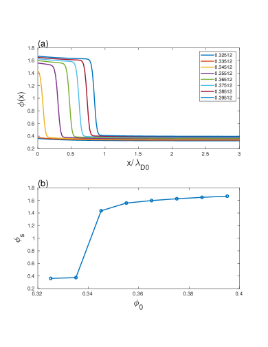
Figure 4: (a) Composition profiles $\phi(\tilde{x})$ for a fluid confined by a charged wall at $\tilde{x}=0$ for several values of bulk composition $\phi_{0}$ (see legend), at fixed temperature and surface voltage. Below the critical composition $\approx 0.34$ the surface is wetted by a vapor while above this composition it is wetted by a liquid. The liquid-vapor interface is always at a finite distance but increases as the composition approaches the binodal value. (b) Surface composition $\phi_{s}$ vs the bulk composition $\phi_{0}$ in part (a). We used $\tilde{V}=2$, $\tilde{c}=0.02$, $\Delta\tilde{\gamma}=0$, and $t=0.9$.

We now lift this assumption and use full profiles calculated numerically. Figure 4 (a) depicts $\phi(\tilde{x})$ for several bulk compositions at fixed $t$ and $\tilde{V}$. At the two lower compositions, the profiles are smoothly varying and the surface has vapor phase. Above the critical composition (in this example $\phi_{0}\approx 0.34$), a first-order transition occurs and the surface is wet by the liquid. At even higher compositions, the vapor-liquid interface moves to larger (but always finite) distances. Part (b) shows the surface composition $\phi_{s}$ vs $\phi_{0}$.

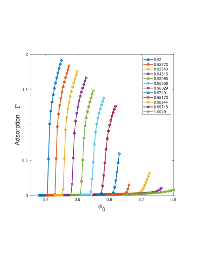
Figure 5: Adsorption curves $\Gamma(\phi_{0})$ at different temperatures $t$ given in the legend. The abrupt change in $\Gamma(\phi_{0})$ is the first-order prewetting transition. We used $\tilde{V}=1$, $\tilde{c}=0.02$, and $\Delta\tilde{\gamma}=0$.

Figure 5 shows the adsorption curves $\Gamma$ at different temperatures and fixed potential. $\Gamma$ is defined as

$$\Gamma=\int_{0}^{\infty}\phi(\tilde{x})d\tilde{x}.$$ (22)

For all temperatures, the values of $\phi_{0}$ used are smaller than the corresponding binodal composition. $\Gamma$ increases with $\phi_{0}$ monotonically and has an abrupt change at a specific composition, signaling the prewetting transition. At temperatures closer to the bulk critical point ($t\lesssim 1$) the change in $\Gamma$ is less abrupt. Across the second-order line the change is continuous but this is not discernible at the parameters used here and is not shown.

Figure 6 is the phase diagram in the $(\phi_{0},t)$ plane for a fixed value of $\tilde{V}$ and a diffuse interface ($\tilde{c}\neq 0$). In these axes, the critical point of the classic van der Waals fluid is at $(1,1)$. The black concave curve is the bulk field-free binodal obtained from the common-tangent construction. The blue line is the first-order transition. Compositions to its left lead to a dry surface while to its right the surface becomes wet. The first order line terminates at a temperature where the transition becomes second order (see Fig. 3). In the numerical scheme using a diffuse interface, $\tilde{c}\neq 0$, it is difficult to reliably find this line and hence it is not shown.

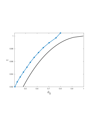
Figure 6: Phase diagram at constant potential. Black line is the binodal curve and blue line is the electro-prewetting line. It terminates at a temperature that is close to $1$ but slightly larger because $\Delta u\neq 0$. We used $\tilde{V}=1$, $\tilde{c}=0.02$, $v_{0}\rho_{c}\Delta u=0.2$, and $\Delta\tilde{\gamma}=0$.

III.3 Analytical profiles and quadratic expansion of the energy

We now seek analytical approximations for the composition profiles and the film energy. At surface potentials smaller than the critical value, the profiles $\phi(\tilde{{\bf r}})$ are smooth and the variation $|\phi(\tilde{{\bf r}})-\phi_{0}|$ is everywhere small. In that case, the free-energy Eq. (5) can be expanded to quadratic order in both $\varphi\equiv\phi-\phi_{0}$ and $\tilde{\psi}^{2}$. The total grand-canonical potential $\Omega$ is

$$\frac{\Omega}{\lambda_{D0}^{3}P_{c}} \approx \phi_{0}\Delta\tilde{\gamma}+\int\left\{\tilde{f}_{\rm vdw}(\phi_{0})-2\tilde{P}\tilde{n}_{0}-\mu_{0}\phi_{0}\right.$$

$$+ \frac{1}{2}\alpha^{2}\tilde{c}^{2}\varphi^{2}+\frac{1}{2}\tilde{c}^{2}(\tilde{\nabla}\varphi)^{2}-\frac{1}{2}M\left(\varepsilon(\phi_{0})+\Delta\varepsilon\varphi\right)(\tilde{\nabla}\tilde{\psi})^{2}$$

$$- \left.\tilde{P}\tilde{n}_{0}[1+v_{0}\rho_{c}\Delta u\varphi]\tilde{\psi}^{2}\right\}{\rm d}\tilde{{\bf r}}+\int\varphi(\tilde{{\bf r}}_{s})\Delta\tilde{\gamma}{\rm d}\tilde{{\bf r}}_{s},$$

where

$$\alpha^{2} = \frac{\tilde{f}_{\rm vdw}^{\prime\prime}(\phi_{0})-2\tilde{P}\tilde{n}_{0}(v_{0}\rho_{c}\Delta u)^{2}}{\tilde{c}^{2}}~{}$$ (24)

is the inverse squared correlation length modified by the presence of the ions (see Appendix A for details). The quantity $\alpha^{2}$ replace the standard bulk $f^{\prime\prime}(\phi)$ term in a Landau-series expansion; it contains a correction to the correlation length due to the preferential solubility of the ions and hints to a change in the bulk critical point [31].

The first line in Eq. (III.3) includes constant terms; the last term in the third line is the change in the surface energy, which is linear in $\varphi$. For the specific case of a van der Waals fluid, the vanishing of the second derivative is written as

$$\frac{8t}{3}\left(\frac{1}{\phi}+\frac{1}{3-\phi}\right)+\frac{8t}{(3-\phi)^{2}}-6-2\tilde{P}\tilde{n}_{0}(v_{0}\rho_{c}\Delta u)^{2}=0.$$

In the bulk, the field vanishes and the third derivative of the free energy is

$$\frac{72t\left(1-\phi\right)}{\left(3-\phi\right)^{3}\phi^{2}}-2\tilde{P}\tilde{n}_{0}(v_{0}\rho_{c}\Delta u)^{3}=0.$$

Treating $v_{0}\rho_{c}\Delta u$ as small and looking to linear order in $\Delta t$ and $\Delta\phi_{c}$, we find that the bulk critical point is shifted according to

$$t_{c} = 1+\Delta t~{}~{}~{}~{}~{}~{}~{}~{}~{}~{}~{}~{}~{}~{}~{}~{}~{}~{}~{}~{}~{}~{}~{}~{}~{}~{}~{}\phi_{c}=1+\Delta\phi_{c},$$ (25)

$$\Delta t = \frac{1}{3}\tilde{P}\tilde{n}_{0}(v_{0}\rho_{c}\Delta u)^{2}~{}~{}~{}~{}~{}~{}~{}~{}~{}\Delta\phi_{c}=\frac{2}{9}\tilde{P}\tilde{n}_{0}(v_{0}\rho_{c}\Delta u)^{3}.$$

One can estimate the magnitude of this shift for water by using $P_{c}=22\times 10^{6}$ Pa, $T_{c}=670^{\circ}$K, $v_{0}\simeq 3\times 10^{-29}$ m³, $\rho_{c}\simeq 10^{28}$ m^-3, and taking $\Delta u=1$ and $\tilde{n}_{0}=0.001$, that is, one ion on every $1000$ water molecules. It then follows that $\Delta T=(1/3)T_{c}\tilde{P}\tilde{n}_{0}(v_{0}\rho_{c}\Delta u)^{2}\simeq 0.1^{\circ}$K.

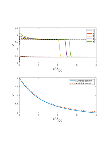
Figure 7: (a) Composition profiles at several values of the surface potential $\tilde{V}$ (see legend). For the two small values of $\tilde{V}$, the profile $\phi(\tilde{x})$ smoothly decreases with increasing $\tilde{x}$. At short distance, $\phi(\tilde{x})$ increases since $\Delta\tilde{\gamma}=0.01$ is positive, favoring the vapor phase. When the surface potential is large enough, $\tilde{V}=3$, $4$, $5$, an electroprewetting transition occurs, with liquid phase at small $\tilde{x}$ coexisting with a vapor at larger distances. Fine dash-dotted horizontal lines are the low and high values of the binodal compositions at the same temperature, $\phi_{b,l}$ and $\phi_{b,h}$, respectively. Lower and higher dashed lines are the linear approximations based on Eq. (29). (b) The numerical (solid) and analytical (dashed) potential profiles $\tilde{\psi}(\tilde{x})$ for $\tilde{V}=2$ of part (a). In both parts, the reduced temperature is $t=0.9$ and $\tilde{c}=0.02$.

We now take the variation of the quadratic energy with respect to $\varphi$ and $\tilde{\psi}$. To lowest order we obtain

$$\alpha^{2}\tilde{c}^{2}\varphi-\tilde{c}^{2}\varphi^{\prime\prime}-\frac{1}{2}M\Delta\tilde{\varepsilon}(\tilde{\nabla}\tilde{\psi})^{2}-\tilde{P}\tilde{n}_{0}v_{0}\rho_{c}\Delta u\tilde{\psi}^{2}=0,$$

(27)

$$M\varepsilon(\phi_{0})\tilde{\nabla}^{2}\tilde{\psi}-2\tilde{P}\tilde{n}_{0}\tilde{\psi}=0.$$

In one dimension, the Poisson equation is readily solved noting that $2\tilde{P}\tilde{n}_{0}/M=1$: $\tilde{\psi}=\tilde{V}e^{-\beta\tilde{x}}$, where $\beta^{2}=1/\varepsilon(\phi_{0})$. The equation for $\varphi$ can now be written as

$$\varphi^{\prime\prime}-\alpha^{2}\varphi = Be^{-2\beta\tilde{x}},$$ (28)

where

$$B = -\frac{M}{2\tilde{c}^{2}}\left(v_{0}\rho_{c}\Delta u+\Delta\varepsilon\beta^{2}\right)\tilde{V}^{2}.$$

The form of the quantity $B$ shows that the preferential solvation, proportional to $\Delta u$, leading to an electrophoretic force on the fluid, appears on the same footing as the “dielectric contrast”, $\Delta\varepsilon\beta^{2}$, in our notation, which leads to a dielectrophoretic force.

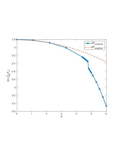
Figure 8: Numerical [solid line, from Eqs. (5) and (7)] and analytical [dashed line, Eq. (33)] film energies as a function of increasing surface potential $\tilde{V}$. The energy decreases monotonically as $\tilde{V}$ increases. For the values of parameters chosen here, the critical electroprewetting potential is $\tilde{V}_{c}\approx 4.75$. When $\tilde{V}<\tilde{V}_{c}$, the analytical approximation matches well the numerical energy; above $\tilde{V}_{c}$ it is not a good approximation as the film energy exhibits a sharp decrease in its value. We used $\Delta\tilde{\gamma}=-0.005$, $t=0.7$, $\tilde{c}=0.1$, and $\phi_{0}=0.99\phi_{b,l}$ for this temperature.

The solution for $\varphi$ obeying the boundary conditions $\tilde{c}^{2}\varphi^{\prime}(0)=\Delta\tilde{\gamma}$ and $\varphi(\infty)=0$ is

$$\varphi = Ae^{-\alpha\tilde{x}}+\frac{B}{4\beta^{2}-\alpha^{2}}e^{-2\beta\tilde{x}},$$ (29)

with

$$A = -\frac{2\beta B}{\alpha(4\beta^{2}-\alpha^{2})}-\frac{\Delta\tilde{\gamma}}{\alpha\tilde{c}^{2}}.$$ (30)

Note that the deviation of the surface composition from the bulk value is

$$\varphi(0)=-\frac{\Delta\tilde{\gamma}}{\alpha\tilde{c}^{2}}-\frac{B}{\alpha(\alpha+2\beta)}.$$ (31)

Since $B$ is negative, when $\Delta\tilde{\gamma}=0$ it follows that $\varphi(0)>0$: The dielectrophoretic and electrophoretic forces are both attracting the liquid to the wall increasing its density there.

We are now in a position to substitute the profiles just obtained back in the energy, to get the integrated energy (see Appendix B for details):

$$\frac{\Omega_{\rm tot}-\Omega_{0}}{\lambda_{D0}^{3}P_{c}} = -\frac{1}{2}M\tilde{V}^{2}/\beta+\frac{1}{2}\tilde{c}^{2}A^{2}\alpha-2\tilde{c}^{2}\frac{AB\beta}{\alpha^{2}-4\beta^{2}}$$

$$- \frac{1}{8}\tilde{c}^{2}\frac{B^{2}}{\beta}\frac{\alpha^{2}-12\beta^{2}}{\left(\alpha^{2}-4\beta^{2}\right)^{2}}+\left(A+\frac{B}{4\beta^{2}-\alpha^{2}}\right)\Delta\tilde{\gamma}.$$

$\Omega_{0}/(\lambda_{D0}^{3}P_{c})=\phi_{0}\Delta\tilde{\gamma}+\int_{0}^{\infty}[\tilde{f}_{\rm vdw}(\phi_{0})-2\tilde{P}\tilde{n}_{0}-\mu_{0}\phi_{0}]{\rm d}\tilde{x}$ is the (infinite) bulk energy.

We further use the relation between $A$ and $B$ in Eq. (30) to eliminate $A$ and express $\Omega_{\rm tot}$ in terms of $B$ and $\Delta\tilde{\gamma}$:

$$\frac{\Omega_{\rm tot}-\Omega_{0}}{\lambda_{D0}^{3}P_{c}} = -\frac{1}{2}M\tilde{V}^{2}/\beta-\frac{1}{8}\frac{B^{2}\tilde{c}^{2}}{\alpha\beta}\frac{\alpha+4\beta}{(\alpha+2\beta)^{2}}$$ (33)

$$- \frac{B\Delta\tilde{\gamma}}{\alpha(\alpha+2\beta)}-\frac{1}{2}\frac{\Delta\tilde{\gamma}^{2}}{\alpha\tilde{c}^{2}}.$$

In the absence of surface potential, $\tilde{V}=0$ and $B\propto\tilde{V}^{2}=0$, and the energy is just the last term. This negative energy is the standard expression, quadratic in $\Delta\tilde{\gamma}$. When the surface has no chemical wetting preference, $\Delta\tilde{\gamma}=0$, the energy is quadratic in the potential. In the general case, a mixed term $\propto B\Delta\tilde{\gamma}$ exists.

Figure 7 shows the profiles $\phi(\tilde{x})$ and $\tilde{\psi}(\tilde{x})$ obtained from a numerical solutions of Eqs. (8)–(10) for varying surface potentials. The bulk composition $\phi_{0}$ was chosen to reflect a stable vapor phase. When $\tilde{V}$ is small ($\tilde{V}=1$ or $2$), the profiles are smooth and $\phi(\tilde{x})$ is always close to its bulk value vapor $\phi_{0}$. In that particular example, close to the surface $\phi$ is smaller due to our choice of positive value of $\Delta\tilde{\gamma}$. However, if the surface potential is large enough ($\tilde{V}=3$, $4$, or $5$), then the electroprewetting phase transition pursues marked by a dense liquid phase at the wall and a vapor phase far from it. The lower thick dashed line is the linear approximation $\phi=\phi_{0}+\varphi$ with a small $\varphi$ taken from Eq. (29), valid before the transition. The higher thick dashed line is a similar approximation $\phi=\phi_{b,h}+\varphi$ with values of $\alpha$ and $\beta$ from:

$$\alpha^{2} = \frac{\tilde{f}_{\rm vdw}^{\prime\prime}(\phi_{b,h})-2\tilde{P}\tilde{n}_{0}(v_{0}\rho_{c}\Delta u)^{2}e^{v_{0}\rho_{c}\Delta u(\phi_{b,h}-\phi_{0})}}{\tilde{c}^{2}},$$

$$\beta^{2} = \frac{e^{v_{0}\rho_{c}\Delta u(\phi_{b,h}-\phi_{0})}}{\tilde{\varepsilon}(\phi_{b,h})}.$$ (34)

In Fig. 8 we present the total integrated energy of the fluid vs $\tilde{V}$ near a slightly hydrophilic surface. The solid line is the numerical value of the energy calculated from the sum of Eqs. (5) and (7). The dashed line is the analytical approximation Eq. (33). The energy decreases as $\tilde{V}$ increases. The numerical and analytical energies are quite similar before the critical prewetting potential ($\tilde{V}_{c}\approx 4.75$). At $\tilde{V}_{c}$, the film energy decreases discontinuously and the analytical approximation fails.

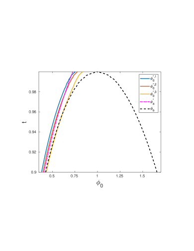
Figure 9: Phase diagram in the $(\phi_{0},t)$ plane. Dashed line is the classical bulk binodal curve $\phi_{b}$ of the van der Waals model. $\phi_{a}^{*}$ is the analytical stability line obtained from Eq. (III.1) with surface potential $\tilde{V}=1$. $\phi_{0}^{*,1}$ is the phase line for $\Delta\tilde{\gamma}=-10^{-3}$ and the same potential. For a given temperature and surface potential, $\phi_{0}^{*,1}$ is the value of $\phi_{0}$ in Eqs. (8)–(10) giving $\phi(0)=\phi_{b,l}$. The two curves $\phi_{0}^{*,2}$ and $\phi_{0}^{*,3}$ are similar but $\Delta\tilde{\gamma}$ is $\Delta\tilde{\gamma}=-5\times 10^{-4}$ and $\Delta\tilde{\gamma}=5\times 10^{-4}$, respectively.

Figure 9 depicts the phase diagram in the $(\phi_{0},t)$ plane with five curves. The dashed line is the bulk van der Waals binodal curve. $\phi_{a}^{*}$ is from the analytical expression from Eq. (III.1). $\phi_{a}^{*}$ is the value of $\phi_{0}$ satisfying this equation for a given value of the surface potential $\tilde{V}=1$ and varying temperatures. Note that due to the approximation used, $\phi_{a}^{*}$ is not sensitive to the value of short-range chemical affinity $\Delta\tilde{\gamma}$. The three other lines are the phase lines $\phi_{0}^{*,i}$ ($i=1$, $2$, $3$) corresponding to the same $\tilde{V}$ and three different values of $\Delta\tilde{\gamma}$. They were obtained by looking for the value of bulk composition $\phi_{0}$ that yields a numerical solution of Eqs. (8)–(10) with $\phi_{s}=\phi_{b,l}$. That is, $\phi_{0}^{*,i}$ are the values of $\phi_{0}$ where a fluid profile whose density at the surface is exactly equal to the (lower) binodal density. When $\Delta\tilde{\gamma}=5\times 10^{-4}$ (orange line), the surface is hydrophobic and the unstable region is small. The surface hydrophobicity is stronger than the field-effect at all temperature except close to the critical point ($t\lesssim 1$). When the surface is hydrophilic, $\Delta\tilde{\gamma}=-5\times 10^{-4}$ (red line), the unstable region is larger. Prewetting occurs even farther away from the binodal at stronger hydrophilicity, $\Delta\tilde{\gamma}=-10^{-3}$ (blue line).

IV Conclusions

We looked at the wetting of a van der Waals fluid model containing dissociated ions near a wall with short-range chemical interaction and long-range electrostatic forces. Density gradients occur because of two forces: ionic screening leads to field gradients and these lead to a dielectrophoretic force tending to “suck” the fluid to the wall. Simultaneously, ions attracted to the wall ‘drag” the fluid with them with a force proportional to $\Delta u$ stemming from their preferential solvation. We calculated the film energy on the mean-field level numerically for all values of surface potential and bulk compositions and analytically for conditions where the variations in the density profiles are small.

The phenomenon discussed here has numerous differences from the classical wetting. In classical wetting, the first integration of the equation for $\phi$ is possible and this gives the profile. The temperature of the “surface critical point” is different from the bulk critical temperature. In the present case, due to the existence of ions and formation of a Debye double layer, the integration is not possible and a profile exists even if the gradient-squared term is absent from the energy ($\tilde{c}=0$). The long-range electrostatic forces give rise to a second-order transition line. A discontinuity in the profile requires the inflection of the bulk energy, that is, the first-order line terminates at $T_{c}$. Non-zero preferential solubility ($\Delta u\neq 0$) changes this, and so does a nonlinear dependence of $\varepsilon$ on $\phi$, but a linear relation $\varepsilon(\phi)$ does not. The second-order line starts from the termination of the first-order line and extends towards the bulk critical point.

The changes to the phase diagram are much larger than those expected by the influence of a uniform field (Landau mechanism). The appreciable change in phase transition temperature can be seen from the upward shift from the binodal temperature, see, for example, Figs. 6 and 9. The shift in $t$, $\Delta t=0.01$–$0.05$, can be translated to a shift in $T$, $\Delta T\simeq 6$–$30^{\circ}$K. One can look at the corresponding shift in pressure by comparing $\Delta T/T_{c}$ to $\Delta P/P_{c}$, and therefore obtain the shift to be $\Delta P\approx 10^{6}$ Pa, that is, about $10$ Atm. The van der Waals model employed here is generally considered to give poor quantitative predictions and cannot be used to reliably predict the numerical values of many physical quantities. Simulations on the molecular level, such as Brownian dynamics or Monte Carlo simulations, would allow to obtain more accurate numerical predictions. We considered the values of both $\varepsilon$ and $\Delta u$ to be such that the liquid is adsorbed at the surface. We leave for a future work to study the competition between these forces when their signs are opposite. In the Earth’s atmosphere, colloidal aggregates and particles are crucial to nucleation of liquid droplets. We believe that our results could be implemented to ion-induced nucleation around charged particles [32, 33, 34, 35, 36] and possibly shed light on unexplained fast nucleation rates reported.

APPENDIX A

In this Appendix we expand the free-energy Eq. (5) to quadratic order in $\varphi\equiv\phi-\phi_{0}$ and $\tilde{\psi}^{2}$. Since $\tilde{n}^{\pm}\approx\tilde{n}_{0}(1\mp\psi+v_{0}\rho_{c}\Delta u\varphi)$ we have

$$\tilde{n}^{+}(\ln(\tilde{n}^{+})-1) \approx \tilde{n}_{0}(\ln\tilde{n}_{0}-1)+\tilde{n}_{0}\ln\tilde{n}_{0}v_{0}\rho_{c}\Delta u\varphi+\frac{1}{2}\tilde{n}_{0}\left(1+\ln\tilde{n}_{0}\right)\left(v_{0}\rho_{c}\Delta u\varphi\right)^{2}$$

$$- \tilde{n}_{0}\ln\tilde{n}_{0}\tilde{\psi}-\tilde{n}_{0}(\ln\tilde{n}_{0}+1)\tilde{\psi}v_{0}\rho_{c}\Delta u\varphi+\frac{1}{2}\tilde{n}_{0}(\ln\tilde{n}_{0}+1)\tilde{\psi}^{2},$$

$$\tilde{n}^{-}(\ln(\tilde{n}^{-})-1) \approx \tilde{n}_{0}(\ln\tilde{n}_{0}-1)+\tilde{n}_{0}\ln\tilde{n}_{0}v_{0}\rho_{c}\Delta u\varphi+\frac{1}{2}\tilde{n}_{0}\left(1+\ln\tilde{n}_{0}\right)\left(v_{0}\rho_{c}\Delta u\varphi\right)^{2}$$

$$+ \tilde{n}_{0}\ln\tilde{n}_{0}\tilde{\psi}+\tilde{n}_{0}(\ln\tilde{n}_{0}+1)\tilde{\psi}v_{0}\rho_{c}\Delta u\varphi+\frac{1}{2}\tilde{n}_{0}(\ln\tilde{n}_{0}+1)\tilde{\psi}^{2},$$

$$\Rightarrow\tilde{n}^{+}(\ln(\tilde{n}^{+})-1) + \tilde{n}^{-}(\ln(\tilde{n}^{-})-1)$$

$$=2\tilde{n}_{0}(\ln\tilde{n}_{0}-1) + 2\tilde{n}_{0}\ln\tilde{n}_{0}\left(v_{0}\rho_{c}\Delta u\varphi\right)+\tilde{n}_{0}(1+\ln\tilde{n}_{0})\left(\tilde{\psi}^{2}+(v_{0}\rho_{c}\Delta u\varphi)^{2}\right).$$ (35)

$$(\tilde{n}^{+}-\tilde{n}^{-})\tilde{\psi}\approx-2\tilde{n}_{0}\tilde{\psi}^{2}-2\tilde{n}_{0}v_{0}\rho_{c}\Delta u\left(\varphi+\frac{1}{2}v_{0}\rho_{c}\Delta u\varphi^{2}\right)\tilde{\psi}^{2}.$$ (36)

$$\left(\tilde{n}^{+}+\tilde{n}^{-}\right)\phi \approx \tilde{n}_{0}\left(1-\tilde{\psi}+v_{0}\rho_{c}\Delta u\varphi+\frac{1}{2}(\tilde{\psi}-v_{0}\rho_{c}\Delta u\varphi)^{2}\right)(\phi_{0}+\varphi)$$ (37)

$$+ \tilde{n}_{0}\left(1+\tilde{\psi}+v_{0}\rho_{c}\Delta u\varphi+\frac{1}{2}(-\tilde{\psi}-v_{0}\rho_{c}\Delta u\varphi)^{2}\right)(\phi_{0}+\varphi)$$

$$= 2\tilde{n}_{0}\phi_{0}$$

$$+ 2\tilde{n}_{0}\varphi+2\tilde{n}_{0}\phi_{0}v_{0}\rho_{c}\Delta u\varphi$$

$$+ \tilde{n}_{0}\phi_{0}\left(\tilde{\psi}^{2}+(v_{0}\rho_{c}\Delta u\varphi)^{2}\right)+2\tilde{n}_{0}v_{0}\rho_{c}\Delta u\varphi^{2}+O(\varphi^{3}).$$

Therefore the free-energy Eq. (5) can be written as

$$\frac{F}{\lambda_{D0}^{3}P_{c}} \approx \int\left\{\tilde{f}_{\rm vdw}(\phi_{0})+\tilde{f}_{\rm vdw}^{\prime}(\phi_{0})\varphi+\frac{1}{2}\tilde{f}_{\rm vdw}^{\prime\prime}(\phi_{0})\varphi^{2}+\frac{1}{2}\tilde{c}^{2}(\tilde{\nabla}\varphi)^{2}\right.$$

$$+ \tilde{P}\left[2\tilde{n}_{0}(\ln\tilde{n}_{0}-1)+2\tilde{n}_{0}\ln\tilde{n}_{0}\left(v_{0}\rho_{c}\Delta u\varphi\right)+\tilde{n}_{0}(1+\ln\tilde{n}_{0})\left(\tilde{\psi}^{2}+(v_{0}\rho_{c}\Delta u\varphi)^{2}\right)\right]$$

$$- \frac{1}{2}M\left(\varepsilon(\phi_{0})+\Delta\varepsilon\varphi\right)(\tilde{\nabla}\tilde{\psi})^{2}-2\tilde{P}\tilde{n}_{0}\ln\tilde{n}_{0}\tilde{\psi}^{2}-2\tilde{P}\tilde{n}_{0}v_{0}\rho_{c}\Delta u\varphi\tilde{\psi}^{2}$$

$$- \left.\tilde{P}v_{0}\rho_{c}\Delta u\left[2\tilde{n}_{0}\phi_{0}+2\tilde{n}_{0}\varphi+2\tilde{n}_{0}\phi_{0}v_{0}\rho_{c}\Delta u\varphi+\tilde{n}_{0}\phi_{0}\left(\tilde{\psi}^{2}+(v_{0}\rho_{c}\Delta u\varphi)^{2}\right)+2\tilde{n}_{0}v_{0}\rho_{c}\Delta u\varphi^{2}\right]\right\}{\rm d}\tilde{{\bf r}}.$$

To this energy we add the chemical potential terms. They are

$$\frac{F_{\mu}}{\lambda_{D0}^{3}P_{c}} = \int\left\{-\mu_{0}(\phi_{0}+\varphi)-\mu^{+}\tilde{n}_{0}\left(1-\tilde{\psi}+v_{0}\rho_{c}\Delta u\varphi+\frac{1}{2}(\tilde{\psi}-v_{0}\rho_{c}\Delta u\varphi)^{2}\right)\right.$$

$$- \left.\mu^{-}\tilde{n}_{0}\left(1+\tilde{\psi}+v_{0}\rho_{c}\Delta u\varphi+\frac{1}{2}(\tilde{\psi}+v_{0}\rho_{c}\Delta u\varphi)^{2}\right)\right\}{\rm d}\tilde{{\bf r}},$$

where

$$\mu_{0} = \tilde{f}^{\prime}_{\rm vdw}(\phi_{0})-2\tilde{P}\tilde{n}_{0}v_{0}\rho_{c}\Delta u,$$

$$\mu^{\pm} = \tilde{P}\left(\ln\tilde{n}_{0}-v_{0}\rho_{c}\Delta u\phi_{0}\right).$$ (38)

The sum $\Omega=F+F_{\mu}$ is

$$\frac{\Omega}{\lambda_{D0}^{3}P_{c}} = \int\left\{\tilde{f}_{\rm vdw}(\phi_{0})+\tilde{f}_{\rm vdw}^{\prime}(\phi_{0})\varphi+\frac{1}{2}\tilde{f}_{\rm vdw}^{\prime\prime}(\phi_{0})\varphi^{2}+\frac{1}{2}\tilde{c}^{2}(\tilde{\nabla}\varphi)^{2}-\frac{1}{2}M\left(\varepsilon(\phi_{0})+\Delta\varepsilon\varphi\right)(\tilde{\nabla}\tilde{\psi})^{2}\right.$$

$$- 2\mu^{\pm}\tilde{n}_{0}+2\tilde{P}\tilde{n}_{0}(\ln\tilde{n}_{0}-1)-\mu_{0}\phi_{0}-2\tilde{P}\tilde{n}_{0}v_{0}\rho_{c}\Delta u\phi_{0}$$

$$+ \left(-\mu_{0}-2\mu^{\pm}\tilde{n}_{0}v_{0}\rho_{c}\Delta u+2\tilde{P}\tilde{n}_{0}v_{0}\rho_{c}\Delta u\ln\tilde{n}_{0}+2\tilde{P}\tilde{n}_{0}v_{0}\rho_{c}\Delta u(-v_{0}\rho_{c}\Delta u\phi_{0}-1)\right)\varphi$$

$$+ \left(-\mu^{\pm}\tilde{n}_{0}(v_{0}\rho_{c}\Delta u)^{2}-\tilde{P}\tilde{n}_{0}(v_{0}\rho_{c}\Delta u)^{2}+\tilde{P}\tilde{n}_{0}(v_{0}\rho_{c}\Delta u)^{2}\ln\tilde{n}_{0}-\tilde{P}\tilde{n}_{0}(v_{0}\rho_{c}\Delta u)^{3}\phi_{0}\right)\varphi^{2}$$

$$+ \left[-\tilde{n}_{0}\left(\mu^{\pm}+\tilde{P}(1-\ln\tilde{n}_{0}+v_{0}\rho_{c}\Delta u\phi_{0})\right)-\tilde{n}_{0}v_{0}\rho_{c}\Delta u\left(\mu^{\pm}+\tilde{P}(1-\ln\tilde{n}_{0}+v_{0}\rho_{c}\Delta u\phi_{0})\right)\varphi\right.$$

$$+ \left.\left.\frac{1}{2}\tilde{n}_{0}(v_{0}\rho_{c}\Delta u)^{2}\left(\mu^{\pm}+\tilde{P}(1-\ln\tilde{n}_{0}+v_{0}\rho_{c}\Delta u\phi_{0})\right)\varphi^{2}\right]\tilde{\psi}^{2}\right\}{\rm d}\tilde{{\bf r}}.$$

The terms $\tilde{f}_{\rm vdw}^{\prime}(\phi_{0})\varphi-\mu_{0}\varphi-2\tilde{P}\tilde{n}_{0}v_{0}\rho_{c}\Delta u\varphi=0$ cancel out, and the surface term $\varphi(0)\Delta\tilde{\gamma}$ is added. The result, after additional cleaning, is Eq. (III.3).

APPENDIX B

In this Appendix we substitute the profiles in Eq. (29) in the quadratic free-energy Eq. (III.3). We note that $\int_{0}^{\infty}\tilde{\psi}^{2}dx=\tilde{V}^{2}/2\beta$ and $\int_{0}^{\infty}\tilde{\psi}^{\prime 2}dx=\tilde{V}^{2}\beta/2$; in addition

$$\int_{0}^{\infty}\varphi^{2}dx = \frac{A^{2}}{2\alpha}-\frac{2AB}{(\alpha-2\beta)(\alpha+2\beta)^{2}}+\frac{B^{2}}{4\beta(\alpha^{2}-4\beta^{2})^{2}},$$

$$\int_{0}^{\infty}\varphi^{\prime 2}dx = \frac{1}{2}A^{2}\alpha-\frac{4AB\alpha\beta}{(2\beta+\alpha)^{2}(\alpha-2\beta)}+\frac{B^{2}\beta}{(4\beta^{2}-\alpha^{2})^{2}},$$

$$\int_{0}^{\infty}\varphi\tilde{\psi}^{2}dx = \frac{1}{4}\tilde{V}^{2}\frac{B+4A\beta(2\beta-\alpha)}{\beta(4\beta^{2}-\alpha^{2})},$$

$$\int_{0}^{\infty}\varphi\tilde{\psi}^{\prime 2}dx = \frac{1}{4}\tilde{V}^{2}\beta\frac{B+4A\beta(2\beta-\alpha)}{4\beta^{2}-\alpha^{2}}.$$

We write $\Omega_{0}/(\lambda_{D0}^{3}P_{c})=\phi_{0}\Delta\tilde{\gamma}+\int_{0}^{\infty}[\tilde{f}_{\rm vdw}(\phi_{0})-2\tilde{P}\tilde{n}_{0}-\mu_{0}\phi_{0}]{\rm d}\tilde{x}$ and use $2\tilde{P}\tilde{n}_{0}=M$:

$$\frac{\Omega-\Omega_{0}}{\lambda_{D0}^{3}P_{c}} = \frac{1}{2}\tilde{c}^{2}\left[\frac{A^{2}\alpha}{2}-\frac{2AB\alpha^{2}}{(\alpha-2\beta)(\alpha+2\beta)^{2}}+\frac{B^{2}\alpha^{2}}{4\beta(\alpha^{2}-4\beta^{2})^{2}}\right]$$

$$+ \frac{1}{2}\tilde{c}^{2}\left[\frac{1}{2}A^{2}\alpha-\frac{4AB\alpha\beta}{(2\beta+\alpha)^{2}(\alpha-2\beta)}+\frac{B^{2}\beta}{(4\beta^{2}-\alpha^{2})^{2}}\right]$$

$$- \frac{1}{4}M\varepsilon(\phi_{0})\tilde{V}^{2}\beta-\frac{1}{8}M\Delta\varepsilon\tilde{V}^{2}\beta\frac{B+4A\beta(2\beta-\alpha)}{4\beta^{2}-\alpha^{2}}$$

$$- \frac{1}{4}M\tilde{V}^{2}/\beta$$

$$- \frac{1}{8}Mv_{0}\rho_{c}\Delta u\tilde{V}^{2}\frac{B+4A\beta(2\beta-\alpha)}{\beta(4\beta^{2}-\alpha^{2})}$$

$$+ \left(A+\frac{B}{4\beta^{2}-\alpha^{2}}\right)\Delta\tilde{\gamma}.$$

$$\frac{\Omega-\Omega_{0}}{\lambda_{D0}^{3}P_{c}} = \frac{1}{2}\tilde{c}^{2}A^{2}\alpha+\frac{1}{2}\tilde{c}^{2}\left[-\frac{2AB\alpha^{2}+4AB\alpha\beta}{(\alpha-2\beta)(\alpha+2\beta)^{2}}+\frac{B^{2}\left(\alpha^{2}+4\beta^{2}\right)}{4\beta(\alpha^{2}-4\beta^{2})^{2}}\right]$$

$$- \frac{1}{8}M\Delta\varepsilon\tilde{V}^{2}\beta\frac{B+4A\beta(2\beta-\alpha)}{4\beta^{2}-\alpha^{2}}$$

$$- \frac{1}{2}M\tilde{V}^{2}/\beta$$

$$- \frac{1}{8}Mv_{0}\rho_{c}\Delta u\tilde{V}^{2}\frac{B+4A\beta(2\beta-\alpha)}{\beta(4\beta^{2}-\alpha^{2})}$$

$$+ \left(A+\frac{B}{4\beta^{2}-\alpha^{2}}\right)\Delta\tilde{\gamma}.$$

Further simplification yields:

$$\frac{\Omega-\Omega_{0}}{\lambda_{D0}^{3}P_{c}} = \frac{1}{2}\tilde{c}^{2}\left(A^{2}\alpha-\frac{2AB\alpha}{\alpha^{2}-4\beta^{2}}+\frac{B^{2}\left(\alpha^{2}+4\beta^{2}\right)}{4\beta\left(\alpha^{2}-4\beta^{2}\right)^{2}}\right)$$

$$- \frac{1}{8}M\tilde{V}^{2}\left(\Delta\varepsilon\beta^{2}+v_{0}\rho_{c}\Delta u\right)\frac{B+4A\beta(2\beta-\alpha)}{\beta\left(4\beta^{2}-\alpha^{2}\right)}$$

$$- \frac{1}{2}M\tilde{V}^{2}/\beta$$

$$+ \left(A+\frac{B}{4\beta^{2}-\alpha^{2}}\right)\Delta\tilde{\gamma}.$$

We now use the definition of $B=-M\left(v_{0}\rho_{c}\Delta u+\Delta\varepsilon\beta^{2}\right)\tilde{V}^{2}/2\tilde{c}^{2}$ on the second line:

$$\frac{\Omega-\Omega_{0}}{\lambda_{D0}^{3}P_{c}} = \frac{1}{2}\tilde{c}^{2}\left(A^{2}\alpha-\frac{2AB\alpha}{\alpha^{2}-4\beta^{2}}+\frac{B^{2}\left(\alpha^{2}+4\beta^{2}\right)}{4\beta\left(\alpha^{2}-4\beta^{2}\right)^{2}}\right)$$

$$+ \frac{1}{4}B\tilde{c}^{2}\frac{B+4A\beta(2\beta-\alpha)}{\beta\left(4\beta^{2}-\alpha^{2}\right)}$$

$$- \frac{1}{2}M\tilde{V}^{2}/\beta$$

$$+ \left(A+\frac{B}{4\beta^{2}-\alpha^{2}}\right)\Delta\tilde{\gamma}.$$

We combine the first and second lines:

$$\frac{\Omega-\Omega_{0}}{\lambda_{D0}^{3}P_{c}}=\frac{1}{2}\tilde{c}^{2}\left(A^{2}\alpha-\frac{4AB\beta}{\alpha^{2}-4\beta^{2}}-\frac{1}{4}\frac{B^{2}\left(\alpha^{2}-12\beta^{2}\right)}{\beta\left(\alpha^{2}-4\beta^{2}\right)^{2}}\right)-\frac{1}{2}M\tilde{V}^{2}/\beta+\left(A+\frac{B}{4\beta^{2}-\alpha^{2}}\right)\Delta\tilde{\gamma}.$$

Equation (III.3) is retrieved.

References

- Landau and Lifshitz [1957] L. D. Landau and E. M. Lifshitz, Electrodynamics of Continuous Media (Nauka, Moscow, 1957).
- Debye and Kleboth [1965] P. Debye and K. Kleboth, Electrical field effect on the critical opalescence, J. Chem. Phys. 42, 3155 (1965).
- Reich and Gordon [1979] S. Reich and J. M. Gordon, Electric field dependence of lower critical phase separation behavior in polymer-polymer mixtures, J. Polym. Sci., Part B: Polym. Phys. 17, 371 (1979).
- Early [1992] M. D. Early, Dielectric constant measurements near the critical point of cyclohexane-aniline., J. Chem. Phys. 96, 641 (1992).
- Wirtz and Fuller [1993] D. Wirtz and G. G. Fuller, Phase transitions induced by electric fields in near-critical polymer solutions, Phys. Rev. Lett. 71, 2236 (1993).
- Orzechowski [1999] K. Orzechowski, Electric field effect on the upper critical solution temperature, Chem. Phys. 240, 275 (1999).
- Orzechowski et al. [2014] K. Orzechowski, M. Adamczyk, A. Wolny, and Y. Tsori, Shift of the critical mixing temperature in strong electric fields. theory and experiment, J. Phys. Chem. B 118, 7187 (2014).
- Tsori [2009] Y. Tsori, Colloquium: Phase transitions in polymers and liquids in electric fields, Rev. Mod. Phys. 81, 1471 (2009).
- Tsori and Leibler [2007] Y. Tsori and L. Leibler, Phase-separation in ion-containing mixtures in electric fields, Proc. Natl. Acad. Sci. U.S.A. 104, 7348 (2007).
- Galanis and Tsori [2013] J. Galanis and Y. Tsori, Mixing-demixing phase diagram for simple liquids in nonuniform electric fields, Phy. Rev. E 88, 10.1103/PhysRevE.88.012304 (2013).
- Galanis and Tsori [2014] J. Galanis and Y. Tsori, Phase separation dynamics of simple liquids in non-uniform electric fields, J. Chem. Phys. 140, 10.1063/1.4869113 (2014).
- Samin and Tsori [2009] S. Samin and Y. Tsori, Stability of binary mixtures in electric field gradients, J. Chem. Phys. 131, 10.1063/1.3257688 (2009).
- Samin and Tsori [2011] S. Samin and Y. Tsori, Vapor-liquid equilibrium in electric field gradients, J. Phys. Chem. B 115, 75 (2011).
- Hefter [2005] G. Hefter, Ion solvation in aqueous?organic mixtures, Pure Appl. Chem. 77, 605 (2005).
- Onuki and Okamoto [2011] A. Onuki and R. Okamoto, Selective solvation effects in phase separation in aqueous mixtures, Curr. Opin. Colloid Interface Sci. 16, 525 (2011).
- Zhang and Cremer [2006] Y. Zhang and P. S. Cremer, Interactions between macromolecules and ions: The hofmeister series, Curr. Opin. Chem. Biol. 10, 658 (2006).
- dos Santos et al. [2010] A. P. dos Santos, A. Diehl, and Y. Levin, Surface tensions, surface potentials, and the hofmeister series of electrolyte solutions, Langmuir 26, 10778 (2010).
- Morag et al. [2013] J. Morag, M. Dishon, and U. Sivan, The governing role of surface hydration in ion specific adsorption to silica: An afm-based account of the hofmeister universality and its reversal, Langmuir 29, 6317 (2013), pMID: 23631425, http://dx.doi.org/10.1021/la400507n .
- Schwierz et al. [2013] N. Schwierz, D. Horinek, and R. R. Netz, Anionic and cationic hofmeister effects on hydrophobic and hydrophilic surfaces, Langmuir 29, 2602 (2013), pMID: 23339330, http://dx.doi.org/10.1021/la303924e .
- Schwierz et al. [2010] N. Schwierz, D. Horinek, and R. R. Netz, Reversed anionic hofmeister series: The interplay of surface charge and surface polarity, Langmuir 26, 7370 (2010), pMID: 20361734, http://dx.doi.org/10.1021/la904397v .
- Jungwirth and Tobias [2006] P. Jungwirth and D. J. Tobias, Specific ion effects at the air/water interface, Chem. Rev. 106, 1259 (2006), http://pubs.acs.org/doi/pdf/10.1021/cr0403741 .
- Levin [2009] Y. Levin, Polarizable ions at interfaces, Phys. Rev. Lett. 102, 147803 (2009).
- Levin et al. [2009] Y. Levin, A. P. dos Santos, and A. Diehl, Ions at the air-water interface: An end to a hundred-year-old mystery?, Phys. Rev. Lett. 103, 257802 (2009).
- Markovich et al. [2015] T. Markovich, D. Andelman, and R. Podgornik, Surface tension of electrolyte interfaces: Ionic specificity within a field-theory approach, J. Chem. Phys. 142, 044702.1 (2015).
- Ben-Yaakov et al. [2011] D. Ben-Yaakov, D. Andelman, and R. Podgornik, Dielectric decrement as a source of ion-specific effects, J. Chem. Phys. 134, 10.1063/1.3549915 (2011).
- Marcus [2002] Y. Marcus, Solvent Mixtures: Properties and Selective Solvation (CRC Press, Boca Raton, FL, 2002).
- Moldover et al. [1979] M. R. Moldover, J. V. Sengers, R. W. Gammon, and R. J. Hocken, Gravity effects in fluids near the gas-liquid critical point, Rev. Mod. Phys. 51, 79 (1979).
- Cahn [1977] J. W. Cahn, Critical point wetting, J. Chem. Phys. 66, 3667 (1977).
- De Gennes [1985] P.-G. De Gennes, Wetting: statics and dynamics, Rev. Mod. Phys. 57, 827 (1985).
- Ebner and Saam [1987] C. Ebner and W. F. Saam, New reentrant wetting phenomena and critical behavior near bulk critical points, Phys. Rev. Lett. 58, 587 (1987).
- Yabunaka and Onuki [2017] S. Yabunaka and A. Onuki, Electric double layer composed of an antagonistic salt in an aqueous mixture: Local charge separation and surface phase transition, Phys. Rev. Lett. 119, 118001 (2017).
- Kirkby et al. [2016] J. Kirkby, J. Duplissy, K. Sengupta, C. Frege, H. Gordon, C. Williamson, M. Heinritzi, M. Simon, C. Yan, J. Almeida, et al., Ion-induced nucleation of pure biogenic particles, Nature 533, 521 (2016).
- Laakso et al. [2002] L. Laakso, J. M. Mäkelä, L. Pirjola, and M. Kulmala, Model studies on ion-induced nucleation in the atmosphere, J. Geophys. Res.: Atmos. 107, AAC (2002).
- Lovejoy et al. [2004] E. Lovejoy, J. Curtius, and K. Froyd, Atmospheric ion-induced nucleation of sulfuric acid and water, J. Geophys. Res.: Atmos. 109 (2004).
- Kroll and Tsori [2021] R. Kroll and Y. Tsori, Liquid nucleation around charged particles in the vapor phase, J. Chem. Phys 155, 174101 (2021).
- Egorov [2004] S. Egorov, Ion solvation dynamics in supercritical fluids, Phys. Rev. Lett. 93, 023004 (2004).