Drying-induced stresses in poroelastic drops on rigid substrates

Abstract

We develop a theory for drying-induced stresses in sessile, poroelastic drops undergoing evaporation on rigid surfaces. Using a lubrication-like approximation, the governing equations of three-dimensional nonlinear poroelasticity are reduced to a single thin-film equation for the drop thickness. We find that thin drops experience compressive elastic stresses but the total in-plane stresses are tensile. The mechanical response of the drop is dictated by the initial profile of the solid skeleton, which controls the in-plane deformation, the dominant components of elastic stress, and sets a limit on the depth of delamination that can potentially occur. Our theory suggests that the alignment of desiccation fractures in colloidal drops is selected by the shape of the drop at the point of gelation. We propose that the emergence of three distinct fracture patterns in dried blood drops is a consequence of a non-monotonic drop profile at gelation. We also show that depletion fronts, which separate wet and dry solid, can invade the drop from the contact line and localise the generation of mechanical stress during drying. Finally, the finite element method is used to explore the stress profiles in drops with large contact angles.

I Introduction

The drying behaviour of thin films and drops is important to a multitude of industries and applications. The presence of a particulate phase introduces appreciable changes to the evaporative process and leads to hydrodynamic and mechanical instabilities, sometimes resulting in cracking. While traditionally viewed as detrimental, the onset of cracking can play an advantageous role in a number of modern applications, from affordable medical diagnostics [1] to high-resolution, high-throughput nano-patterning [2]. With such a broad range of applications, there is a growing need for efficient and accurate modelling capabilities of the stresses accompanying the evaporation of particle-laden films and drops. Yet considerable complexity arises in these drying systems from the delicate interplay between capillarity, thermocapillarity, heat and mass transfer, contact lines (undergoing pinning and de-pinning), and, crucially, the formation of a poroelastic network, which controls the formation of cracks and their morphology. In this paper, we focus on the development of a theory for drying-induced stresses in sessile, poroelastic drops undergoing evaporation on rigid surfaces.

Many important patterning behaviours manifest during the evaporation of droplets [3] due to the interaction between evaporation-driven flows and the contact line [4]. The commonly encountered ‘coffee-ring’ stain is one such example, where evaporation in the presence of a non-volatile solute promotes the appearance of a distinctly inhomogeneous deposit. Deegan et al. [5, 6, 7] first explained the origin of this effect by the presence of an increased evaporative flux at the contact line, coupled with a resultant capillary-induced restoration flow.

Crack formation in drying colloidal drops is thought to be a multi-step process originating from the coffee-ring effect [8, 9]. The radially outwards capillary flow transports colloids to the pinned contact line where they accumulate due to weak, counteracting diffusive effects [10]. Gelation occurs once the particle concentration exceeds a critical value, resulting in the local transformation of the liquid drop into a poroelastic solid; the porous elastic material then has an elastic skeleton with interconnected pores containing fluid. A gelation front consequently emerges from the contact line and propagates towards the drop centre [11]. Mechanical stresses develop in the gelled region because of the competing effects of evaporation-driven contraction of the solid skeleton and its adhesion to the substrate. Cracks therefore emerge as a mechanism to relieve mechanical stress.

Experiments have shown that a myriad of fracture patterns can occur during droplet evaporation [12]. When an aqueous drop with silica nanoparticles dries, fractures typically nucleate at the contact line and travel radially inwards, following the gelation front. These fractures divide the deposit into an array of ‘petals’ that simultaneously delaminate from the substrate, resulting in the entire solid ‘blooming’ into a structure that resembles a lotus flower [13, 14]. In the case of dried blood drops, the solid deposit often has an orthoradial fracture at the contact line, an annular region with several radial fractures, and a central zone with smaller-scale fractures with no preferred orientation [15]. Extensive experimental research has been carried out to elucidate the dependence of the fracture pattern on the contact angle [16, 17], drying rate [18, 19, 20], substrate deformability [21], and particle hydrophobicity [22] and concentration [23, 24]. However, a detailed theoretical description of stress generation in drying colloidal drops is lacking, with treatments relying on scaling analyses [25] or one-dimensional models that do not capture the evolving and non-uniform thickness of the drop [20, 26].

Our work will deploy three-dimensional nonlinear poroelasticity to build a comprehensive model of drying-induced mechanical stresses in drops with a pre-existing solid structure. Moreover, a lubrication-like approximation will be invoked to systematically reduce the governing equations. Poroelasticity theory is based on the premise that the solid phase is arranged into a porous and deformation structure referred to as the ‘solid skeleton’. Biot developed the theory of poroelasticity [27, 28, 29] to account for the two-way coupling between the deformation of the solid skeleton and fluid flow within the pore space. The theory formalised by Biot assumes the deformation of the solid skeleton is infinitesimal and thus describes the solid skeleton as a linearly elastic material. When the solid deformation is no longer infinitesimal, one must derive poroelastic models in the framework of nonlinear elasticity [30, 31]. The lubrication approximation has been used in tandem with the theory of poroelasticity [32, 33] to study thin films for various applications such as CO₂ sequestration [34], imbibition [35], soft contact [36, 37], and biomechanics [38, 39].

By combining poroelasticity with the lubrication approximation, we are able to provide novel physical insights into the internal droplet dynamics. In the case of axisymmetric drops with circular contact lines, we find that the initial profile of the poroelastic drop plays a critical role in selecting the modes of in-plane deformation, thereby determining whether the radial or hoop stresses dominate. Our work suggests that the fracture patterns appearing in drying colloidal drops are dictated by the shape of the drop at the point of gelation, in agreement with the experimental observations of Bourrianne et al. [24]. By comparing the magnitude of the radial and hoop stresses, we correctly predict the emergence of three distinct fracture patterns in dried drops of blood [11]. We also find that the drop profile affects the depth of delamination, which may not reach the drop centre, in line with the experiments of Osman et al. [26]. We show that a sharp decrease in the permeability during drying can result in the formation of depletion fronts that invade the bulk of the drop from the contact line and localise the accumulation of stresses. Finally, finite element simulations are used to calculate the stress profiles in poroelastic drops with large contact angles. We find that many of the conclusions obtained from the reduced model still apply.

The rest of this paper is organised as follows. In Section II, details of the problem formulation and non-dimensionalisation are provided. The governing equations are asymptotically reduced in Section III. The results are discussed in Section IV, while Section V is devoted to the concluding remarks.

II Problem formulation

We consider a drop of fluid consisting of a volatile solvent (e.g. water) and a non-volatile colloidal component (e.g. nanoparticles) that dries on a horizontal non-deformable solid substrate. We envision the colloids as having formed a poroelastic solid from which evaporation occurs. The contact line is assumed to remain pinned, which is in agreement with experiments, and the time-dependent contact angle $\varphi(t)$ is assumed to be small. The characteristic height and lateral extent (e.g. the radius) of the drop are denoted by $H$ and $R$, respectively, where $H/R\ll 1$. We work within the framework of nonlinear poroelasticity [31] to account for large deformations during drying. We also assume that the drop remains bonded to the underlying substrate and thus neglect delamination processes that can potentially occur.

II.1 Kinematics

The governing equations are formulated in terms of Eulerian coordinates $\boldsymbol{x}=x_{i}\boldsymbol{e}_{i}$ associated with the current (deformed) configuration, where $\boldsymbol{e}_{i}$ are Cartesian basis vectors and summation over repeated indices is implied. We let $\boldsymbol{X}=X_{i}\boldsymbol{e}_{i}$ denote Lagrangian coordinates associated with the initial (undeformed) configuration of the drop. During drying, the solid element originally located at $\boldsymbol{X}$ is displaced to $\boldsymbol{x}$, thereby generating a displacement $\boldsymbol{u}^{s}=\boldsymbol{x}-\boldsymbol{X}(\boldsymbol{x},t)$. The deformation gradient tensor $\boldsymbol{\mathsf{F}}$ and its determinant $J=\det\boldsymbol{\mathsf{F}}$ describe the distortion and volumetric changes of material elements, respectively. In Eulerian coordinates, the deformation gradient tensor is most readily expressed in terms of its inverse as

$$\boldsymbol{\mathsf{F}}^{-1}=\nabla\boldsymbol{X}=\boldsymbol{\mathsf{I}}-\nabla\boldsymbol{u}^{s},$$ (1)

where $\nabla$ is the spatial gradient taken with respect to the Eulerian coordinates $\boldsymbol{x}$. We adopt the convention that $\nabla\boldsymbol{u}^{s}=(\partial u_{i}^{s}/\partial x_{j})\,\boldsymbol{e}_{i}\otimes\boldsymbol{e}_{j}$. The velocity of the fluid and solid are written as $\boldsymbol{v}^{f}$ and $\boldsymbol{v}^{s}$, respectively. In Eulerian formulations of nonlinear elasticity, the rate of change of displacement is linked to the velocity by the relationship

$$\frac{\partial\boldsymbol{u}^{s}}{\partial t}+(\boldsymbol{v}^{s}\cdot\nabla)\boldsymbol{u}^{s}=\boldsymbol{v}^{s},$$ (2)

where $\boldsymbol{u}^{s}={\bf 0}$ when $t=0$.

II.2 Balance laws

The composition of the mixture is described by the volume fractions of fluid and solid, $\phi^{f}$ and $\phi^{s}$, respectively. Conservation of liquid and solid yield

$$\frac{\partial\phi^{f}}{\partial t}+\nabla\cdot(\phi^{f}\boldsymbol{v}^{f}) =0,$$ (3a)

$$\frac{\partial\phi^{s}}{\partial t}+\nabla\cdot(\phi^{s}\boldsymbol{v}^{s}) =0.$$ (3b)

In deriving (3), it has been assumed that the densities of the solid skeleton and the fluid are constant, that is, both phases are incompressible. Furthermore, it is assumed that no volume change occurs upon mixing and that material elements only consist of solid and fluid, the latter of which leads to the condition

$$\phi^{f}+\phi^{s} =1.$$ (4)

Since the pore space is only occupied by fluid, the volume fraction of fluid $\phi^{f}$ also represents the porosity of the solid. Due to the incompressibility of the fluid and solid, volumetric changes in material elements can only be due to imbibition or depletion of fluid within the pore space, leading to the relationship

$$J=\det\boldsymbol{\mathsf{F}}=\frac{1-\phi^{f}_{0}}{1-\phi^{f}},$$ (5)

where $\phi^{f}_{0}$ represents the fluid fraction in the initial undeformed configuration. For simplicity, we assume that $\phi^{f}_{0}$ is spatially uniform. The Jacobian determinant $J$ describes the local contraction of the solid skeleton ($J<1$) that occurs due to the loss of fluid from the pore space ($\phi^{f}<\phi^{f}_{0}$). If the porosity $\phi^{f}$ remains spatially uniform during drying, then the Jacobian determinant can be written in terms of the total drop volume $V$ as $J(t)=V(t)/V(0)$.

The fluid within the pore space is assumed to be transported by pressure gradients. Hence, we impose Darcy’s law,

$$\phi^{f}(\boldsymbol{v}^{f}-\boldsymbol{v}^{s}) =-\frac{k(\phi^{f})}{\mu_{f}}\nabla p,$$ (6)

where $k$ is the permeability of the solid skeleton, $\mu_{f}$ is the fluid viscosity, and $p$ is the pressure. The contraction of the solid matrix during drying will reduce the pore size and hence decrease the permeability. Deformation-driven changes in the permeability are captured through its dependence on the porosity. In particular, we adopt a normalised Kozeny–Carmen law [40, 41] for the permeability given by

$$\frac{k(\phi^{f})}{k_{0}}=\frac{(1-\phi^{f}_{0})^{2}}{(\phi^{f}_{0})^{3}}\frac{(\phi^{f})^{3}}{(1-\phi^{f})^{2}},$$ (7)

where $k_{0}$ is the permeability of the initial configuration.

Conservation of momentum for the two-phase mixture yields

$$\nabla\cdot\boldsymbol{\sigma} =\nabla p,$$ (8)

where $\boldsymbol{\sigma}$ is the effective (Terzaghi) elastic stress tensor of the solid [30], which commonly appears in soil mechanics [27, 42]. The solid skeleton is assumed to be isotropic and obey a neo-Hookean equation of state. The elastic component of the stress tensor can be written as

$$\begin{split}\boldsymbol{\sigma}=\frac{\nu E}{(1+\nu)(1-2\nu)}(J-1)\boldsymbol{\mathsf{I}}+\frac{E}{2(1+\nu)J}(\boldsymbol{\mathsf{B}}-\boldsymbol{\mathsf{I}}),\end{split}$$ (9)

where $E$ is the Young’s modulus, $\nu$ is Poisson’s ratio (both assumed constant), $\boldsymbol{\mathsf{I}}$ is the identity tensor, and $\boldsymbol{\mathsf{B}}=\boldsymbol{\mathsf{F}}\boldsymbol{\mathsf{F}}^{T}$ is the left Cauchy–Green tensor. In the limit of small deformations, $\nabla\boldsymbol{u}^{s}\ll 1$, we find that $\boldsymbol{\mathsf{F}}\sim\boldsymbol{\mathsf{I}}+\nabla\boldsymbol{u}^{s}$, which implies that $\boldsymbol{\mathsf{B}}\sim\boldsymbol{\mathsf{I}}+\nabla\boldsymbol{u}^{s}+(\nabla\boldsymbol{u}^{s})^{T}$ and $J=\det\boldsymbol{\mathsf{F}}\sim 1+\nabla\cdot\boldsymbol{u}^{s}$. Hence, the stress-strain relation (9) reduces to

$$\boldsymbol{\sigma}\sim \frac{\nu E}{(1+\nu)(1-2\nu)}(\nabla\cdot\boldsymbol{u}^{s})\boldsymbol{\mathsf{I}}$$

$$\quad+\frac{E}{2(1+\nu)}\,\left(\nabla\boldsymbol{u}^{s}+(\nabla\boldsymbol{u}^{s})^{T}\right),$$ (10)

thus recovering linear elasticity.

It is convenient to decompose vector and tensor quantities into in-plane and transverse components that are parallel and perpendicular to the substrate, respectively. We let $x_{3}=z$ and $X_{3}=Z$ denote the transverse Eulerian and Lagrangian coordinates, respectively, and let $\boldsymbol{e}_{3}=\boldsymbol{e}_{z}$ be the corresponding basis vector. If $\boldsymbol{a}=a_{i}\boldsymbol{e}_{i}$ denotes an arbitrary vector, then we write $\boldsymbol{a}=\boldsymbol{a}_{\parallel}+a_{z}\boldsymbol{e}_{z}$, where $\boldsymbol{a}_{\parallel}=a_{\alpha}\boldsymbol{e}_{\alpha}$ is a vector of the in-plane components and $a_{z}=a_{3}$ is the transverse component; here we adopt the convention that Greek indices are equal to 1 or 2. Similarly, we introduce the in-plane gradient operator $\nabla_{\parallel}=\nabla-\boldsymbol{e}_{z}\,\partial/\partial z$. The symmetric elastic stress tensor $\boldsymbol{\mathsf{\sigma}}$ is written in terms of its in-plane components $\boldsymbol{\mathsf{\sigma}}_{\parallel}=\sigma_{\alpha\beta}\boldsymbol{e}_{\alpha}\otimes\boldsymbol{e}_{\beta}$, transverse shear components $\boldsymbol{\sigma}_{\perp}=\sigma_{\alpha 3}\boldsymbol{e}_{\alpha}$, and vertical component $\sigma_{zz}$ as $\boldsymbol{\mathsf{\sigma}}=\boldsymbol{\mathsf{\sigma}}_{\parallel}+\boldsymbol{\sigma}_{\perp}\otimes\boldsymbol{e}_{z}+\boldsymbol{e}_{z}\otimes\boldsymbol{\sigma}_{\perp}+\sigma_{zz}\boldsymbol{e}_{z}\otimes\boldsymbol{e}_{z}$. Similar decompositions will be used for other tensorial quantities as well.

II.3 Boundary and initial conditions

We assume that the solid skeleton perfectly adheres to the rigid substrate, resulting in a no-displacement condition

$$\boldsymbol{u}^{s}={\bf 0},\quad z=0.$$ (11)

In addition, the substrate is taken to be impermeable; therefore,

$$\boldsymbol{v}^{f}\cdot\boldsymbol{e}_{z}=0,\quad z=0.$$ (12)

The static contact line of the drop is denoted by the curve $\boldsymbol{r}^{c}_{\parallel}$ and defined by the equation

$$h=0,\quad\boldsymbol{x}_{\parallel}=\boldsymbol{r}^{c}_{\parallel}.$$ (13)

The kinematic boundary conditions for the fluid and solid phase at the free surface are given by

$$\rho_{f}\phi^{f}(\boldsymbol{v}^{f}\cdot\boldsymbol{n}-v_{n}) =\phi^{f}q_{\mathrm{e}}, \quad z =h(\boldsymbol{x}_{\parallel},t),$$ (14a)

$$\rho_{s}\phi^{s}(\boldsymbol{v}^{s}\cdot\boldsymbol{n}-v_{n}) =0, \quad z =h(\boldsymbol{x}_{\parallel},t),$$ (14b)

where $\rho_{f}$ and $\rho_{s}$ are the densities of the fluid and solid, respectively; $q_{\mathrm{e}}=q_{\mathrm{e}}(\phi^{f})$ is the evaporative mass flux which depends on the surface composition; and $v_{n}$ is the normal velocity of the free surface, defined as

$$v_{n}=\frac{1}{(1+|\nabla_{\parallel}h|^{2})^{1/2}}\frac{\partial h}{\partial t}.$$ (15)

Continuity of stress at the drop surface is given by

$$\boldsymbol{\mathsf{\sigma}}\cdot\boldsymbol{n}-p\boldsymbol{n}=\boldsymbol{0},\quad z=h(\boldsymbol{x}_{\parallel},t),$$ (16)

where the atmospheric pressure has been set to zero. Similar boundary conditions on the stress have been used by other researchers when modelling drying-induced stresses in colloidal suspensions [43, 44]. The initial conditions for the fluid fraction, displacement, and drop thickness are given by

$$\phi^{f}(\boldsymbol{x},0) =\phi^{f}_{0},$$ (17a)

$$\boldsymbol{u}^{s}(\boldsymbol{x},0) =\boldsymbol{0},$$ (17b)

$$h(\boldsymbol{x}_{\parallel},0) =h_{0}(\boldsymbol{x}_{\parallel}).$$ (17c)

The initial conditions can be placed in the context of drying colloidal dispersions by connecting the quantities $h_{0}$ and $\phi^{f}_{0}$ to the profile of the drop and the volume fraction of liquid at the point of gelation. The gel point depends on the nature of the colloids as well as the evaporation conditions, as these control the possible arrangements of particles (e.g. random close packing, face-centred cubic). The experimental observation of gelation fronts implies that different regions of the drop undergo the sol-gel transition at different times, making it difficult to define a profile for $h_{0}$. However, some insights can be obtained from the shape of the solid deposit that remains on the substrate when drying is complete. Anyfantakis et al. [22] examined the drying of aqueous drops containing silica nanoparticles; by increasing the hydrophobicity of the nanoparticles, they observed that the final deposit takes on a parabolic profile. Therefore, the colloids likely remained uniformly dispersed during drying, which would have resulted in a homogeneous gelation when the drop had a parabolic profile. However, by decreasing the hydrophobicity of the particles, the deposit had a non-monotonic profile. Given the different profiles that might arise during drying, we will treat $h_{0}$ as a parameter with the aim of elucidating the role it plays in determining the poromechanical response of the drop.

II.4 Scaling and non-dimensionalisation

We scale spatial quantities according to $\boldsymbol{x}_{\parallel}\sim R$, $z\sim H$, $h\sim H$, and define $\epsilon=H/R\ll 1$. For the liquid, we choose the usual lubrication scales for the velocity, $\boldsymbol{v}^{f}_{\parallel}\sim V$ and $v^{f}_{z}\sim\epsilon V$, where the velocity scale $V$ will be defined below. We use an advective time scale given by $t\sim R/V$.

To facilitate identifying appropriate scales for the solid, we assume that the linear stress-strain relation given by (10) applies. Balancing $v^{s}_{z}$ with $\partial h/\partial t$ in the kinematic boundary condition (14b) implies that $v^{s}_{z}\sim\epsilon V$. Moreover, balancing $\partial u_{z}^{s}/\partial t$ with $v^{s}_{z}$ in the vertical component of (2) gives a scale for the vertical displacement: $u_{z}^{s}\sim H$. A scale for the vertical normal stress can then be obtained as $\sigma_{zz}\sim E\,\partial u_{z}^{s}/\partial z\sim E$. We postulate that large horizontal contractions of the solid skeleton are prohibited by its adhesion to the substrate. Therefore, the removal of solvent will drive a predominantly vertical contraction of the solid skeleton. The elastic stress that is generated by this vertical contraction, $\sigma_{zz}$, must be balanced by the pressure, $p$, resulting in $p\sim\sigma_{zz}\sim E$. A scale for the horizontal displacements can be obtained through a consideration of the horizontal momentum balance for the mixture. As in lubrication theory, we expect the horizontal pressure gradient to generate a shear stress. Therefore, we balance $\partial\boldsymbol{\sigma}_{\perp}/\partial z$ with $\nabla_{\parallel}p$ which implies that $\boldsymbol{\sigma}_{\perp}\sim\epsilon E$. The shear stress also scales like $\boldsymbol{\sigma}_{\perp}\sim E\,\partial\boldsymbol{u}^{s}_{\parallel}/\partial z$; thus, we find that $\partial\boldsymbol{u}^{s}_{\parallel}/\partial z\sim\epsilon$. In light of the no-slip condition for the solid, this balance implies that $\boldsymbol{u}^{s}_{\parallel}\sim\epsilon H$ and hence $\boldsymbol{v}^{s}_{\parallel}\sim\epsilon^{2}V$. The in-plane components of the stress tensor can be scaled as $\boldsymbol{\mathsf{\sigma}}_{\parallel}\sim E$. Finally, the velocity scale is determined from the horizontal component of Darcy’s law, which gives $V=(k_{0}/\mu_{f})(E/R)$.

Under this scaling, the non-dimensional displacement gradient is

$$\nabla\boldsymbol{u}^{s}=\epsilon^{2}\nabla_{\parallel}\boldsymbol{u}^{s}_{\parallel}+\epsilon\left(\frac{\partial\boldsymbol{u}^{s}_{\parallel}}{\partial z}\otimes\boldsymbol{e}_{z}+\boldsymbol{e}_{z}\otimes\nabla_{\parallel}u_{z}^{s}\right)$$

$$\quad+\frac{\partial u_{z}^{s}}{\partial z}\boldsymbol{e}_{z}\otimes\boldsymbol{e}_{z},$$ (18)

which shows that in-plane and shear strains will be small. The non-dimensional form of the elastic stress tensor is $\boldsymbol{\mathsf{\sigma}}=\boldsymbol{\mathsf{\sigma}}_{\parallel}+\sigma_{zz}\boldsymbol{e}_{z}\otimes\boldsymbol{e}_{z}+\epsilon(\boldsymbol{\sigma}_{\perp}\otimes\boldsymbol{e}_{z}+\boldsymbol{e}_{z}\otimes\boldsymbol{\sigma}_{\perp})$.

II.4.1 Non-dimensional bulk equations

The rescaled conservation equations for the volume fractions are given by

$$\frac{\partial\phi^{f}}{\partial t}+\nabla_{\parallel}\cdot\left(\phi^{f}\boldsymbol{v}^{f}_{\parallel}\right)+\frac{\partial}{\partial z}\left(\phi^{f}v^{f}_{z}\right) =0,$$ (19a)

$$\frac{\partial\phi^{s}}{\partial t}+\epsilon^{2}\nabla_{\parallel}\cdot\left(\phi^{s}\boldsymbol{v}^{s}_{\parallel}\right)+\frac{\partial}{\partial z}\left(\phi^{s}v^{s}_{z}\right) =0.$$ (19b)

Thus, fluid is transported in both the horizontal and vertical directions. The solid, however, is predominantly transported in the vertical direction, suggesting that a uniaxial mode of deformation occurs. The components of the solid velocity can be obtained from

$$\frac{\partial\boldsymbol{u}^{s}_{\parallel}}{\partial t}+\epsilon^{2}\boldsymbol{v}^{s}_{\parallel}\cdot\nabla_{\parallel}\boldsymbol{u}^{s}_{\parallel}+v^{s}_{z}\frac{\partial\boldsymbol{u}^{s}_{\parallel}}{\partial z}=\boldsymbol{v}^{s}_{\parallel},$$ (20a)

$$\frac{\partial u_{z}^{s}}{\partial t}+\epsilon^{2}\boldsymbol{v}^{s}_{\parallel}\cdot\nabla_{\parallel}u_{z}^{s}+v^{s}_{z}\frac{\partial u_{z}^{s}}{\partial z}=v^{s}_{z}.$$ (20b)

Darcy’s law (6) can be written in component form as

$$\phi^{f}(\boldsymbol{v}^{f}_{\parallel}-\epsilon^{2}\boldsymbol{v}^{s}_{\parallel}) =-k(\phi^{f})\nabla_{\parallel}p,$$ (21a)

$$\epsilon^{2}\phi^{f}(v^{f}_{z}-v^{s}_{z}) =-k(\phi^{f})\frac{\partial p}{\partial z},$$ (21b)

which shows that vertical gradients in the pressure will be weak. The in-plane motion of the solid skeleton plays a sub-dominant role in (21a) and can be neglected. Consequently, the problems describing the in-plane transport of solid and fluid decouple. The momentum balance for the mixture (8) is

$$\nabla_{\parallel}\cdot\boldsymbol{\mathsf{\sigma}}_{\parallel}+\frac{\partial\boldsymbol{\sigma}_{\perp}}{\partial z} =\nabla_{\parallel}p,$$ (22a)

$$\epsilon^{2}\nabla_{\parallel}\cdot\boldsymbol{\sigma}_{\perp}+\frac{\partial\sigma_{zz}}{\partial z} =\frac{\partial p}{\partial z}.$$ (22b)

The lubrication approximation for poroelastic solids therefore leads to a different stress balance than for viscous fluids by bringing the in-plane stresses $\boldsymbol{\mathsf{\sigma}}_{\parallel}$ and the vertical normal stress $\sigma_{zz}$ into the leading-order problem.

II.4.2 Non-dimensional boundary and initial conditions

The non-dimensional adhesion and no-flux conditions are the same as in (11) and (12). The kinematic boundary conditions become

$$\frac{\partial h}{\partial t}+\boldsymbol{v}^{f}_{\parallel}\cdot\nabla_{\parallel}h-v^{f}_{z}=-\mathcal{Q}q(\phi^{f})\mathcal{A},\,\,\,\,z=h(\boldsymbol{x}_{\parallel},t),$$ (23a)

$$\frac{\partial h}{\partial t}+\epsilon^{2}\boldsymbol{v}^{s}_{\parallel}\cdot\nabla_{\parallel}h-v^{s}_{z}=0,\quad z=h(\boldsymbol{x}_{\parallel},t),$$ (23b)

where $\mathcal{Q}=q_{0}/(\rho_{f}V\epsilon)$, $q_{0}=q_{e}(\phi^{f}_{0})$ is the initial evaporative mass flux, and $\mathcal{A}=\left(1+\epsilon^{2}|\nabla_{\parallel}h|^{2}\right)^{1/2}$. The non-dimensional parameter $\mathcal{Q}$ plays the role of a Péclet number by characterising the relative rate of evaporation to bulk fluid transport. The stress balances at the free surface are given by

$$-\boldsymbol{\mathsf{\sigma}}_{\parallel}\cdot\nabla_{\parallel}h+\boldsymbol{\sigma}_{\perp}+p\nabla_{\parallel}h =\boldsymbol{0}, \quad z =h(\boldsymbol{x}_{\parallel},t),$$ (24a)

$$-\epsilon^{2}\boldsymbol{\sigma}_{\perp}\cdot\nabla_{\parallel}h+\sigma_{zz}-p =0, \quad z =h(\boldsymbol{x}_{\parallel},t).$$ (24b)

The initial conditions for the drop profile, porosity, and displacements are $h=h_{0}(\boldsymbol{x}_{\parallel})$, $\phi^{f}=\phi^{f}_{0}$, $\boldsymbol{u}^{s}_{\parallel}=\boldsymbol{0}$, and $u_{z}^{s}=0$ when $t=0$.

II.5 Parameter estimation

Giorgiutti–Dauphiné and Pauchard [20] conducted experiments on colloidal drops consisting of silica nanoparticles in water. They reported values of $k_{0}\sim 10^{-19}$ m², $E\sim 1$ GPa, $\mu_{f}\sim 10^{-3}$ Pa s, and $R\sim 1$ mm. The initial contact angle $\varphi_{0}$ ranged from $30^{\circ}$ to $40^{\circ}$, leading to values of $\epsilon\sim\varphi_{0}$ in the range of 0.5 to 0.7. The evaporation velocity, $V_{e}\sim q_{0}/\rho_{f}$, can be inferred from their measurements of the cracking time and is found to be roughly $10^{-9}$ m s^-1. A conservative estimate of the Péclet number based on a value of $\epsilon=0.1$ is then $\mathcal{Q}\sim 10^{-3}$. Osman et al. [26] reported similar parameter values for their experiments: $k_{0}\sim 10^{-20}$ m², $V_{e}\sim 10^{-8}$ m s^-1, $\mu_{f}\sim 10^{-3}$ Pa s, and $R\sim 1$ mm. The Young’s modulus and contact angles were not measured. However, since their colloidal dispersions were also based on silica nanoparticles, we estimate that $E\sim 1$ GPa. The Péclet number can be parameterised in terms of the initial contact angle as $\mathcal{Q}\sim 10^{-3}\,\varphi_{0}^{-1}$ and is expected to be small. Finally, in the case of drying blood drops, Sobac and Brutin [9] reported that $R=4.3$ mm, $V_{e}\simeq 9\cdot 10^{-8}$ m s^-1, and $\varphi_{0}=15^{\circ}$. Moreover, they estimated that the diffusivity of fluid through the poroelastic solid was roughly $D_{w}\simeq 3\cdot 10^{-8}$ m² s^-1, which leads to a velocity scale of $V\sim D_{w}/R\simeq 7\cdot 10^{-6}$ m s^-1. The corresponding Péclet number is $\mathcal{Q}\sim 0.05$.

III Asymptotic reduction

The dimensionless model is asymptotically reduced by taking the limit as $\epsilon\to 0$. The reduction can be decomposed into two main steps. First, the mechanical problem is solved in terms of the fluid fraction. Second, the transport problems for the fluid and solid are simplified and then combined into a thin-film-like equation for the drop thickness.

The reduction of the mechanical problem begins with a consideration of the rescaled displacement gradient (18) and the deformation gradient tensor (1). By taking $\epsilon\to 0$ in (18) and substituting the result in (1), the leading-order contribution to the deformation gradient tensor can be written as $\boldsymbol{\mathsf{F}}=\boldsymbol{\mathsf{I}}_{\parallel}+J\boldsymbol{e}_{z}\otimes\boldsymbol{e}_{z}$, where $\boldsymbol{\mathsf{I}}_{\parallel}=\boldsymbol{e}_{\alpha}\otimes\boldsymbol{e}_{\alpha}$ is the in-plane identity tensor and

$$J=\det\boldsymbol{\mathsf{F}}=\left(1-\frac{\partial u_{z}^{s}}{\partial z}\right)^{-1}.$$ (25)

The Jacobian determinant $J$ in (25) must also satisfy (5). The asymptotic reduction of the deformation gradient tensor $\boldsymbol{\mathsf{F}}$ shows that, to leading order, the drop undergoes uniaxial deformation along the vertical direction. The leading-order components of the elastic stress tensor are

$$\boldsymbol{\mathsf{\sigma}}_{\parallel} =\frac{\nu}{(1+\nu)(1-2\nu)}(J-1)\boldsymbol{\mathsf{I}}_{\parallel},$$ (26a)

$$\boldsymbol{\sigma}_{\perp} =\frac{1}{2(1+\nu)}\left(J\frac{\partial\boldsymbol{u}^{s}_{\parallel}}{\partial z}+\nabla_{\parallel}u_{z}^{s}\right),$$ (26b)

$$\sigma_{zz} =\frac{1}{1+\nu}\left[\frac{1}{2}(J-J^{-1})+\frac{\nu}{1-2\nu}(J-1)\right].$$ (26c)

By integrating the $O(1)$ contributions to the vertical stress balance (22b), we observe that the pressure is equal to the vertical normal stress,

$$p=\sigma_{zz}=\frac{1}{1+\nu}\left[\frac{1}{2}(J-J^{-1})+\frac{\nu}{1-2\nu}(J-1)\right].$$ (27)

Taking $\epsilon\to 0$ in (21b) shows that the pressure $p$ is independent of $z$ to leading order. Consequently, we deduce that $\sigma_{zz}$, $J$, and hence $\phi^{f}$ are also independent of $z$. The horizontal stress balance (22a) can now be integrated and the stress-free condition (24a) imposed to find

$$\boldsymbol{\sigma}_{\perp}=\frac{1}{2(1+\nu)}\nabla_{\parallel}\left((h-z)(J^{-1}-J)\right).$$ (28)

Equating (26b) and (28) leads to a differential equation for the in-plane components of the solid displacement $\boldsymbol{u}^{s}_{\parallel}$. Furthermore, (25) provides an equation for the vertical displacement $u_{z}^{s}$. Upon solving these equations and imposing $\boldsymbol{u}^{s}=\boldsymbol{0}$ at $z=0$, we find that the displacements are given by

$$\boldsymbol{u}^{s}_{\parallel} =\frac{1}{2}\,z^{2}\,\nabla_{\parallel}(\log J)+zJ^{-1}\nabla_{\parallel}\left(h(J^{-1}-J)\right),$$ (29a)

$$u_{z}^{s} =(1-J^{-1})z.$$ (29b)

At this point, the mechanical problem has been completely solved in terms of the Jacobian determinant $J$, which is linked to the fluid fraction via (5).

At leading order, the conservation law for the fluid (19a) becomes

$$\frac{\partial\phi^{f}}{\partial t}+\nabla_{\parallel}\cdot(\phi^{f}\boldsymbol{v}^{f}_{\parallel})+\phi^{f}\frac{\partial v^{f}_{z}}{\partial z}=0.$$ (30)

Integrating (30) across the thickness of the drop and using the impermeability condition (12) and the kinematic boundary condition (23a) leads to

$$\frac{\partial}{\partial t}(h\phi^{f})+\nabla_{\parallel}\cdot(h\phi^{f}\boldsymbol{v}^{f}_{\parallel})=-\mathcal{Q}\phi^{f}q(\phi^{f}).$$ (31)

Similarly, from the conservation of solid (19b), we find that

$$\frac{\partial}{\partial t}(h\phi^{s})=0$$ (32)

to leading order. By integrating (32) and using the definition of $J$ from (5), we obtain

$$h=Jh_{0}.$$ (33)

Equation (33) reflects the uniaxial mode of deformation that the drop experiences and states that volumetric changes in material elements can only be accommodated through variations in the film thickness $h$. Adding (31) and (32) and using Darcy’s law (21a) gives

$$\frac{\partial h}{\partial t}=\nabla_{\parallel}\cdot\left[k(\phi^{f})h\nabla_{\parallel}p\right]-\mathcal{Q}\phi^{f}q(\phi^{f}).$$ (34)

By using (27) and (33) to write $p=\sigma_{zz}(J)$ and $J=h/h_{0}$, respectively, (34) can be formulated as a thin-film-like equation

$$\frac{\partial h}{\partial t}=\nabla_{\parallel}\cdot\left[k(\phi^{f})h\sigma_{zz}^{\prime}\left(\frac{h}{h_{0}}\right)\nabla_{\parallel}\left(\frac{h}{h_{0}}\right)\right]-\mathcal{Q}\phi^{f}q(\phi^{f}),$$ (35a)

where $$\sigma_{zz}^{\prime}(J)=\mathrm{d}\sigma_{zz}(J)/\mathrm{d}J \phi^{f}=1-(1-\phi_{f,0})(h_{0}/h)$$ and the solvent fraction is given by . The thin-film equation (35a) can be solved using the boundary and initial conditions

$$h =0, \quad\boldsymbol{x}_{\parallel} =\boldsymbol{r}^{c}_{\parallel};$$ (35b)

$$h =h_{0}(\boldsymbol{x}_{\parallel}), \quad t =0.$$ (35c)

Once the drop thickness $h$ is calculated, the Jacobian determinant $J$ can be computed from (33) and used to evaluate the elastic stresses and displacements given by (26)–(29).

III.1 The slow-evaporation limit

The parameter estimates from Sec. II.5 indicate that the Péclet number $\mathcal{Q}$ is typically small, implying that fluid loss due to evaporation is slow relative to the rate at which fluid is replenished by bulk transport. This separation of time scales can be used to further reduce the model. By rescaling time as $t=\mathcal{Q}^{-1}\tau$ and taking $\mathcal{Q}\to 0$, we can deduce from (35a) and (33) that $h/h_{0}$ and hence $J$ must be spatially uniform. This permits the film thickness to be written as $h(\boldsymbol{x}_{\parallel},\tau)=J(\tau)h_{0}(\boldsymbol{x}_{\parallel})$. Consequently, the fluid fraction $\phi^{f}$ must also be independent of space in order to satisfy the incompressibility condition (5). To determine the time dependence of $J$, we integrate (35a) over the contact surface to obtain

$$\frac{\mathrm{d}J}{\mathrm{d}\tau}=-\frac{A_{0}\phi^{f}q(\phi^{f})}{V_{0}},$$ (36)

where $A_{0}$ and $V_{0}$ are the (non-dimensional) area of the contact surface and the initial volume of the drop, respectively, and $\phi^{f}=1-(1-\phi_{f,0})/J$. Equation (36) can be recast into a differential equation for the volume of the drop $V(\tau)$ using the relation $J(\tau)=V(\tau)/V_{0}$.

IV The poromechanics of drying

The solutions of the asymptotically reduced model provide new insights into the poromechanics of drying drops. We first analyse and interpret the solutions for the stress. We then explore the mechanics of drying in the limit of slow evaporation, corresponding to vanishingly small Péclet numbers $\mathcal{Q}$. Numerical simulations are used to study the dynamics for moderate evaporation rates characterised by Péclet numbers that are $O(1)$ in size. Finally, we use finite element simulations to examine the stresses that arise when the contact angle is not small.

IV.1 Analysis of drying-induced stresses

A key feature of the asymptotic reduction is that it allows for a straightforward determination and interpretation of the stresses that are generated during drying. The total stress within the poroelastic drop is characterised by the Cauchy stress tensor $\boldsymbol{\mathsf{T}}=\boldsymbol{\mathsf{\sigma}}-p\boldsymbol{\mathsf{I}}$ and can therefore be decomposed into an elastic stress associated with deformations of the solid skeleton and an isotropic contribution arising from the fluid. Since drying leads to a loss of volume ($J<1$), we see from (26a) that in-plane elastic stresses $\boldsymbol{\mathsf{\sigma}}_{\parallel}$ are compressive. The origin of these compressive stresses can be understood by drawing on the analogy between the drying-induced contraction of the solid skeleton and the vertical compression of a slab of elastic material. Due to the Poisson effect, vertical compression of a slab will drive a lateral (or in-plane) expansion. However, if the slab is bonded to a substrate, then lateral expansion is constrained and a compressive stress is generated to resist lateral deformation. An examination of the total in-plane stresses, defined by

$$\boldsymbol{\mathsf{T}}_{\parallel}=\boldsymbol{\mathsf{\sigma}}_{\parallel}-p\boldsymbol{\mathsf{I}}_{\parallel}=\frac{1}{2(1+\nu)}(J^{-1}-J)\boldsymbol{\mathsf{I}}_{\parallel},$$ (37)

reveals they are tensile due to the negative pressure counteracting the elastic stresses. The combination of a tensile total stress and a compressive elastic stress is consistent with the findings of Bouchaudy and Salmon [43], who report similar mechanics in a one-dimensional setting.

The generation of tensile in-plane stresses leads to a mechanism for fracture, which is commonly observed during the drying of complex colloidal suspensions. However, the isotropic form of the in-plane stress tensor (37) prohibits the leading-order problem from providing any information about the orientation of nucleated fractures, which we expect to be perpendicular to the directions of maximal stress. Any mechanism that could select a preferential direction for fracture must therefore manifest in higher-order contributions to the stress tensor and, as a result, be relatively weak.

Drying-induced stresses can trigger the delamination of the drop from rigid substrates, in which case knowledge of the traction exerted by the drop on the substrate is crucial. The non-dimensional traction is defined as $\boldsymbol{\mathcal{T}}=\boldsymbol{\mathsf{T}}|_{z=0}\cdot\boldsymbol{e}_{z}$. The in-plane components of the traction, which are generated from elastic shear stresses, are readily computed from (28) and found to be

$$\boldsymbol{\mathcal{T}}_{\parallel}=\frac{1}{2(1+\nu)}\nabla_{\parallel}\left(h(J^{-1}-J)\right).$$ (38a)

To determine the leading-order component of the vertical traction $$\mathcal{T}_{z}$$, we integrate (22b) across the thickness of the drop and impose the stress-free condition (24b) to obtain

$$\mathcal{T}_{z}=\frac{\epsilon^{2}}{4(1+\nu)}\nabla_{\parallel}^{2}\left(h^{2}(J^{-1}-J)\right).$$ (38b)

The vertical traction (38b) can be interpreted as the adhesive stress required for the drop to remain bonded to the substrate during drying. Positive and negative values of $\mathcal{T}_{z}$ imply that the drop is pulling upwards and pushing downwards on the substrate, respectively. Due to the prefactor of $\epsilon^{2}\sim\varphi_{0}^{2}$ appearing in (38b), thinner drops with smaller contact angles will be less prone to delamination, provided this occurs once $\mathcal{T}_{z}$ exceeds a critical threshold. To the best of our knowledge, the contact-angle dependence of delamination has not been investigated experimentally.

IV.2 Mechanics in the slow-evaporation limit

Significant insight into the mechanics of drying can be obtained by considering the slow-evaporation limit, as the spatial uniformity of the Jacobian determinant $J$ enables the asymptotic solutions to be greatly simplified. Due to the monotonic decrease in the drop volume $V$ in time, we can use $J(t)=V(t)/V_{0}$ as a proxy for time, where $J$ decreases from $J=1$ when $t=0$ to a steady-state value of $J=J_{\infty}<1$ as $t\to\infty$. For simplicity, we focus on the case of axisymmetric drops with circular contact lines.

The radial displacement can be computed from (29a) and is found to be

$$u^{s}_{r}=z(J^{-1}-J)\frac{\mathrm{d}h_{0}}{\mathrm{d}r}.$$ (39)

Consequently, the radial and orthoradial motion of the solid skeleton is controlled by the initial geometry of the drop, which is encoded in the functional form of $h_{0}$. In locations where the initial profile has a negative slope, $\mathrm{d}h_{0}/\mathrm{d}r<0$, solid elements are displaced towards the drop centre ($u^{s}_{r}<0$) and undergo orthoradial compression ($u^{s}_{r}/r<0$). However, if the initial profile has a positive slope, $\mathrm{d}h_{0}/\mathrm{d}r>0$, then solid elements are displaced towards the contact line ($u^{s}_{r}>0$) and undergo orthoradial expansion ($u^{s}_{r}/r>0$). Similarly, the initial curvature of the solid skeleton, $\mathrm{d}^{2}h_{0}/\mathrm{d}r^{2}$, controls the mode of radial deformation. Solid elements experience a radial compression ($\partial u^{s}_{r}/\partial r<0$) if the curvature is negative and a radial expansion ($\partial u^{s}_{r}/\partial r>0$) if the curvature is positive.

The compressive and extensional modes of radial and orthoradial deformation lead to small differences in the radial and hoop stresses. Although small, these differences can establish a preferential direction for nucleated fractures. By calculating the higher-order terms in the elastic stress tensor, we find that the difference between the radial and hoop stress can be expressed as $\mathsf{T}_{rr}-\mathsf{T}_{\theta\theta}=\sigma_{rr}-\sigma_{\theta\theta}=\epsilon^{2}(1+\nu)^{-1}\mathcal{S}(r,z)$, where

$$\mathcal{S}=\frac{\partial u^{s}_{r}}{\partial r}-\frac{u^{s}_{r}}{r}+J\frac{\partial u^{s}_{r}}{\partial z}\frac{\partial u_{z}^{s}}{\partial r}+\frac{J^{2}}{2}\left(\frac{\partial u^{s}_{r}}{\partial z}\right)^{2}.$$ (40)

The first two terms on the right-hand side of (40) capture the competition between linear radial and orthoradial strains, and they would be present if the model had been formulated in terms of linear elasticity. The final two terms on the right-hand side of (40) arise from geometric nonlinearities associated with finite strains. Substituting the expression for the radial displacement (39) and the vertical displacement (29b) into (40) leads to

$$\mathcal{S}=(J^{-1}-J)z\left(\frac{\mathrm{d}^{2}h_{0}}{\mathrm{d}r^{2}}-\frac{1}{r}\frac{\mathrm{d}h_{0}}{\mathrm{d}r}\right)+\frac{(J^{2}-1)^{2}}{2}\left(\frac{\mathrm{d}h_{0}}{\mathrm{d}r}\right)^{2}.$$ (41)

Using (41), it is straightforward to explore how different drop profiles $h_{0}$ affect the competition between radial and orthoradial stress generation.

Near the contact line, the initial profile of the drop can be locally represented as a linear function with negative gradient. The resulting value of $\mathcal{S}$ will be positive, indicating that the radial stress dominates the hoop stress. Consequently, fractures will have a slight preference to align with (be parallel to) the orthoradial direction. Due to $\mathsf{T}_{rr}-\mathsf{T}_{\theta\theta}$ being proportional to $\epsilon^{2}\sim\varphi_{0}^{2}$, the strength of the orthoradial alignment should increase with the initial contact angle. Observations of similar qualitative trends were made in the experimental work of Carle and Brutin [16, Fig. 4] where increases in the initial contact angle led to increasingly prominent orthoradial fractures at the contact line.

Understanding the competition between the radial and hoop stresses away from the contact line requires specific knowledge of the initial profile of the poroelastic drop. Parabolic profiles for $h_{0}$ represent a special case and lead to the first bracketed term in (41) vanishing, implying that the radial and orthoradial strains are identical in the limit of linear elasticity and can only be distinguished by considering a nonlinear theory. Although the value of $\mathcal{S}$ is always positive for parabolic drops, the prefactor of the final term will be small and thus any preferential orientation of fractures will be very weak. The drying experiments by Anyfantakis et al. [22] support this prediction: the solid deposits that were parabolic in shape were patterned by disordered fractures with no clear orientation. In this case, the parabolic profile is likely a result of the drops remaining homogeneous during drying.

We therefore postulate that the alignment of nucleated fractures is due to the heterogeneous gelation of drops and the creation of poroelastic skeletons with non-parabolic profiles. Sobac and Brutin [9] measured the profile of a dried deposit that was patterned by strongly aligned fractures. The deposit thickness was non-monotonic and found to generally increase towards the contact line until a maximum was reached, after which the thickness rapidly decreased to zero; see Fig. 1 (a). The dried deposit exhibited three distinct fracture patterns: (I) near the contact line there was a large orthoradial fracture; (II) away from the contact line there was an annular region where fractures were predominantly aligned with the radial direction; and (III) there was a central region with non-oriented fractures. An image of the dried deposit showing the three fracture patterns is provided in Fig. 1 (b).

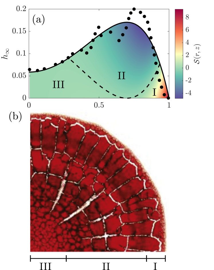
Figure 1: The alignment of fractures is driven by the deposit profile. (a) The steady-state profile of a dried blood drop. Circles represent experimental data from Sobac and Brutin [9] and the solid line is a polynomial fit. The superimposed heatmap illustrates the difference between the radial and hoop stresses $\mathcal{S}=\epsilon^{-2}(1+\nu)(\sigma_{rr}-\sigma_{\theta\theta})$. The black dashed line is the $\mathcal{S}=0$ level set. The three regions correspond to (I) a dominant radial stress (orthoradial fractures), (II) a dominant orthoradial stress (radial fractures) and (III) similar stresses (non-oriented fractures). (b) The deposit associated with the profile in panel (a), showing the three fracture patterns suggested by the asymptotic theory. This figure has been adapted from Sobac and Brutin [9].

The three fracture patterns observed by Sobac and Brutin [9] can be rationalised by the poroelastic model. Doing so requires reconstructing the profile of the drop at the point of gelation, which is achieved using the relation $J=h/h_{0}=(1-\phi^{f}_{0})/(1-\phi^{f})$ and taking $\phi^{f}$ and $h$ to be the equilibrium fluid fraction $\phi^{f}_{\infty}$ and drop profile $h_{\infty}$, respectively. Solving for the initial profile $h_{0}$ gives

$$h_{0}(r)\simeq\left(\frac{1-\phi^{f}_{\infty}}{1-\phi^{f}_{0}}\right)h_{\infty}(r).$$ (42)

Sobac and Brutin [11] estimate that the first fractures occur when the solid fraction is roughly 30%. Therefore, we take the gel point to be $\phi^{f}_{0}\simeq 0.7$. In addition, the solid deposit is assumed to be completely dry, $\phi^{f}_{\infty}\simeq 0$. A smooth function for $h_{\infty}$ is obtained by fitting a polynomial to the experimentally measured profile, resulting in the solid black curve shown in Fig. 1 (a). Using the reconstruction of $h_{0}$ provided by (42), we calculate the difference between the radial and hoop stress via (41) and plot the values of $\mathcal{S}$ as a heatmap in Fig. 1 (a). As predicted, there is a region near the contact line where the radial stress dominates ($\mathcal{S}>0$), resulting in the orthoradial fracture associated with pattern (I). However, there is also an intermediate region centred about the maximum of the deposit thickness where the hoop stress dominates ($\mathcal{S}<0$) and the onset of the radially aligned fractures associated with pattern (II) is expected. Finally, near the drop centre, the value of $\mathcal{S}$ is very close to zero, suggesting the emergence of non-oriented fractures observed in pattern (III).

The model predicts that the appearance of multiple fracture patterns will be a generic feature of poroelastic skeletons that have a non-monotonic initial profile. Near a maximum in the profile, where $\mathrm{d}h_{0}/\mathrm{d}r\simeq 0$ and $\mathrm{d}^{2}h_{0}/\mathrm{d}r^{2}<0$, the hoop stress will dominate the radial stress ($\mathcal{S}<0$), suggesting the emergence of radially aligned fractures. Conversely, local minima in the profile would lead to orthoradially aligned fractures. The presence of multiple maxima and minima in the deposit profile shown in Fig. 1 (a) could explain the sequential realignment of fractures that is seen in Fig. 1 (b).

For slowly evaporating drops, the normal component of the traction reduces to

$$\mathcal{T}_{z}=\frac{\epsilon^{2}}{4(1+\nu)}\frac{J^{2}(J^{-1}-J)}{r}\frac{\mathrm{d}}{\mathrm{d}r}\left[r\frac{\mathrm{d}}{\mathrm{d}r}\left(h_{0}^{2}\right)\right].$$ (43)

The competition between the decrease in the drop height, captured through $J^{2}$, and the increase in elastic stress, captured through $J^{-1}-J$, results in a non-monotonic evolution of the traction that reaches a maximum value when $J=2^{-1/2}\simeq 0.71$. There are two ramifications of this finite maximum. Firstly, it implies that delamination is not guaranteed to occur. Secondly, if delamination does occur, then the propagating delamination front may not reach the drop centre by the end of the drying process. In fact, the drop only pulls upwards on the substrate in locations where the curvature of $h_{0}^{2}$ is positive. For drops with initially parabolic profiles, $h_{0}=1-r^{2}$, the traction is positive for $r>2^{-1/2}$, which sets a theoretical maximum on the depth of delamination.

Osman et al. [26] experimentally observed a limited depth of delamination in drying colloidal drops. Using a simple model, they argued that heterogeneous gelation leads to a poroelastic ‘foot’ developing at the contact line, the length of which controls the depth of delamination. Our complementary theory predicts that even a fully gelled drop could only undergo a partial degree of delamination. When combined, these two theories suggest that the extent of delamination ultimately arises from an intricate interplay between the horizontal growth of the poroelastic solid as well as its shape.

IV.3 Numerical simulations

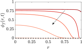
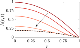
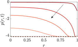
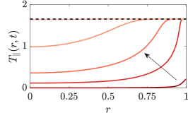
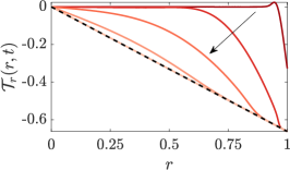
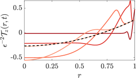
Figure 2: The dynamics of a drying poroelastic drop at a moderate evaporation rate ($\mathcal{Q}=1$). The spatio-temporal evolution of the (a) fluid fraction (porosity), (b) drop thickness, (c) pressure, (d) total in-plane stress, (e) radial and (f) vertical traction on the substrate. The parameter values are $\nu=0.45$, $\phi^{f}_{0}=0.80$, and $q(\phi^{f})\equiv 1$. The solutions are shown at times $t=0.01$, $0.2$, $0.5$, $1$, and $2$. Arrows show the direction of time; the dashed black lines denote the steady states.

The poromechanics that occur for larger Péclet numbers are explored via numerical simulations of the thin-film equation (35) in an axisymmetric geometry. The initial profile of the drop is assumed to be parabolic; thus, we take $h_{0}(r)=1-r^{2}$. For simplicity, the non-dimensional evaporative mass flux is taken to be a constant, $q(\phi^{f})\equiv 1$. As a result, all of the fluid will evaporate from the pores of the solid. The consequences of this simplifying assumption on the dynamics will be discussed below.

The first case we consider corresponds to a moderate rate of evaporation with $\mathcal{Q}=1$. For Péclet numbers $\mathcal{Q}$ that are $O(1)$ in size, the time scale of fluid depletion due to evaporation is commensurate with the time scale of fluid replenishment due to bulk transport. Thus, the generation of composition gradients within the material is to be expected. The initial fluid fraction, or porosity, is set to $\phi^{f}_{0}=0.80$ and the Poisson’s ratio is taken to be $\nu=0.45$. The evolution of the fluid fraction indicates there is a rapid loss of fluid near the contact line, which results in a completely collapsed (fluid-free) solid; see Fig. 2 (a). Due to the sharp decrease in the permeability with the porosity, fluid from the bulk is prohibited from replenishing that which is lost due to evaporation. As the drying process continues, a depletion front invades the drop from the contact line while the fluid content in the bulk decreases with a weak composition gradient. The motion of the depletion front can be detected in the evolution of the drop thickness. Upstream of the front, the drop thickness remains stationary because it has converged to its steady-state profile, while downstream of the front, the drop thickness continues to decrease as fluid is removed from the pore space; see Fig. 2 (b).

The formation of a depletion front plays a significant role in the mechanical response of the drop. The localised removal of fluid from regions near the contact line triggers a vertical compression of the solid skeleton and leads to a large decrease in the pressure, as seen in Fig. 2 (c). This zone of negative pressure propagates into the bulk following the depletion front. In turn, the negative pressure generates tensile stresses $\boldsymbol{\mathsf{T}}_{\parallel}=T_{\parallel}\boldsymbol{\mathsf{I}}_{\parallel}$ in both the radial and orthoradial directions that increasingly penetrate into the bulk with time; see Fig. 2 (d).

The radial traction can be expressed as $\mathcal{T}_{r}=\partial(hT_{\parallel})/\partial r$, which is simply the gradient of the vertically integrated, total radial stress. Thus, the behaviour of the radial traction largely mirrors that of the radial stress: a sharp gradient develops near the contact line and propagates inwards, as shown in Fig. 2 (e). However, unlike the radial stress, the radial traction settles into a non-uniform steady state due to the gradients in the drop thickness. The negative values of the radial traction imply that the substrate is being pulled towards the drop centre. The vertical traction $\mathcal{T}_{z}$ exhibits non-monotonic behaviour in time, which is likely due to the same competition between the decrease in drop height and generation of elastic stress that is captured in Eqn (43). Regions near the contact line experience an upwards force ($\mathcal{T}_{z}>0$) that acts to pull the drop off the substrate and trigger delamination, whereas central regions of the drop push on the substrate ($\mathcal{T}_{z}<0$) and enhance its adhesion; see Fig. 2 (f).

Larger evaporation rates drive the emergence of non-parabolic drop shapes that result in the hoop stress exceeding the radial stress. By computing the rescaled stress difference $\mathcal{S}$ given by (40), we find that a localised region appears at the contact line where the hoop stress exceeds the radial stress ($\mathcal{S}<0$); see Fig. 3 (a). This localised is referred to as the “hoop zone”. As time increases, the hoop zone propagates along the free surface of the drop towards the centre, and, at the contact line, the radial stress overtakes the hoop stress ($\mathcal{S}>0$); see Fig. 3 (b). As the drop completely dries out, the hoop zone dissipates and the radial stress dominates across the entirety of the drop, as seen in Fig. 3 (c). The propagating depletion front separates the hoop zone from the region dominated by the radial stress. The region behind (upstream of) the depletion front is fluid-free and the drop profile is simply a rescaled version of the initial parabolic profile, $h(r,t)\simeq(1-\phi^{f}_{0})h_{0}(r)$; thus, the radial stress dominates, in accordance with (41). Ahead (downstream) of the depletion front, the drop profile becomes non-parabolic due to the non-uniform removal of fluid, thus leading to the hoop zone.

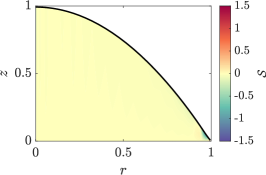
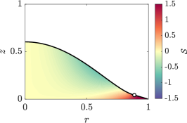
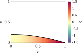
Figure 3: Moderate evaporation rates can lead to the hoop stress exceeding the radial stress in initially parabolic drops. The rescaled difference between the radial and hoop stress $\mathcal{S}=\epsilon^{-2}(1+\nu)(\sigma_{rr}-\sigma_{\theta\theta})$ defined by (40) is shown as a heatmap at times (a) $t=0.01$, (b) $t=0.5$, and (c) $t=2$. The drop profile $h(r,t)$ is shown as the solid black line. The white circle in (b) depicts the position of the depletion front $r_{f}(t)$, defined by $\phi^{f}(r_{f}(t),t)=0.01$. The parameter values are $\mathcal{Q}=1$, $\nu=0.45$, $\phi^{f}_{0}=0.80$, and $q(\phi^{f})=1$.

We now turn our attention to the drop dynamics that occur for slower rates of evaporation by considering the case when $\mathcal{Q}=0.1$. We first consider a drop with the same parameters as in Fig. 2 by setting $\nu=0.45$ and $\phi^{f}_{0}=0.80$. The fluid fraction initially decreases while remaining approximately uniform throughout the drop, see Fig. 4 (a), which is consistent with the findings of the slow-evaporation limit. The homogeneous drying of the drop gives rise to roughly uniform in-plane stresses as well, as shown in Fig. 4 (b). The in-plane stresses, in turn, generate a vertical traction with a roughly parabolic initial profile; see Fig. 4 (c). Eventually, the loss of fluid triggers a sharp decrease in the permeability. Weak gradients in the fluid fraction near the contact line are amplified, resulting in a propagating depletion front; see Fig. 4 (a).

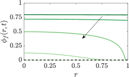
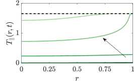
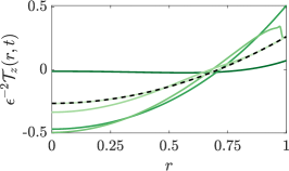
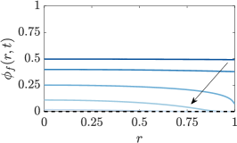
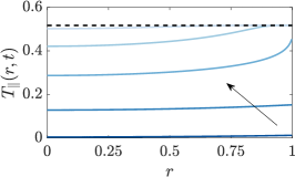
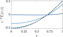
Figure 4: Drop dynamics with a small evaporation rate ($\mathcal{Q}=0.1$). In panels (a)–(c), the initial fluid fraction is $\phi^{f}_{0}=0.80$. In panels (d)–(f), the initial fluid fraction is $\phi^{f}_{0}=0.50$. In all panels, $\nu=0.45$, $q(\phi^{f})\equiv 1$, and the solutions are shown at times $t=0.1$, $2$, $5$, $10$, and $20$. Arrows show the direction of time; the dashed black lines denote the steady states.

Decreasing the initial fluid fraction to $\phi^{f}_{0}=0.5$ and keeping the other parameters fixed leads to qualitatively similar dynamics to those seen in Fig. 4 (a)–(c). However, in this case, the depletion front is more diffuse (Fig. 4 (d)) and the in-plane stresses $T_{\parallel}$ are smaller (Fig. 4 (e)) due to the solid skeleton undergoing less volumetric contraction; recall from (5) that $J=1-\phi^{f}_{0}$ at the steady state. The vertical traction monotonically approaches its steady-state profile (Fig. 4 (g)), which is larger in magnitude than the case when $\phi^{f}_{0}=0.8$ due to the smaller change in drop thickness.

In all of the cases considered so far, it has been assumed that evaporation completely dries the solid, removing all fluid from within the pore space. Relaxing this assumption, so that some fluid remains, will curtail the decrease in the permeability. This will result in weaker gradients in the fluid fraction and, consequently, in all of the other quantities as well. Moreover, it may prohibit the formation of a depletion front altogether.

IV.4 Drops with large contact angle

The finite element method is used to compute the steady-state stress distribution in axisymmetric drops with large contact angles. Under the steady-state assumption, the full time-dependent model described in Sec. II reduces to the equilibrium equations of nonlinear elasticity, $\nabla\cdot\boldsymbol{\mathsf{\sigma}}=\nabla p$, with an incompressibility constraint $J=J_{0}$. The constant $J_{0}<1$ describes the volumetric contraction due to drying. The governing equations are solved in the reference configuration. The finite element method is implemented with FEniCS [45, 46] using P2-P1 elements for displacement and pressure, respectively. In all of the simulations, the initial profile of the drop is taken to be a parabola that is represented in dimensional form as $h_{0}(r)/R=\epsilon\left(1-(r/R)^{2}\right)$. The initial contact angle satisfies $\tan\varphi_{0}=2\epsilon$ and thus $\varphi_{0}\sim 2\epsilon$ for $\epsilon\ll 1$. In addition, we set $J_{0}=1/2$, corresponding to a drop that has shed half of its volume.

We first compute the steady-state drop thickness $h_{\infty}$ for a range of aspect ratios $\epsilon=H/R$. When $\epsilon=0.1$ and $0.2$ ($\varphi_{0}=11^{\circ}$ and $22^{\circ}$), the drops have parabolic profiles that are in good agreement the asymptotic theory; see Fig. 5 (a). However, as $\epsilon$ increases to 0.4 and then to 0.8 ($\varphi_{0}=39^{\circ}$ and $58^{\circ}$), deviations from a parabolic profile begin to emerge. The profile that arises when $\epsilon=0.8$ closely resembles that seen by Pauchard and Allain [47] when studying drying colloidal drops with contact angles on the order of 45^∘. When the contact angle is large, the solid skeleton is generally further away from the substrate and hence less influenced by the no-slip (perfect adhesion) condition. Thus, drying leads to greater radial displacements. However, the radial displacement is constrained near $r=0$ due to the assumption of axisymmetry. The net result is that solid near the contact line is displaced inwards and, in order to conserve solid volume, the vertical contraction of the drop near the centre is reduced.

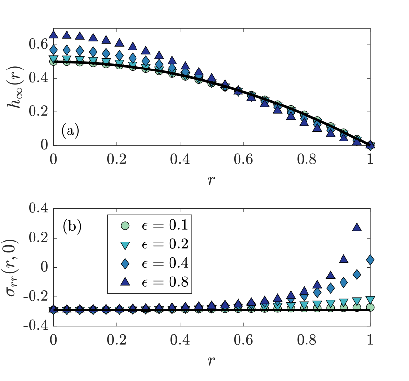
Figure 5: The (a) equilibrium drop thickness $h_{\infty}$ and (b) radial elastic stress along the substrate for different drop aspect ratios $\epsilon=H/R$. Symbols denote quantities computed using the finite element method. The solid black lines denote asymptotic solutions. The legend applies to both panels.

Increasing the contact angle also leads to marked changes in the radial elastic stress $\sigma_{rr}$. When $\epsilon=0.1$ and $0.2$, the radial elastic stress along the substrate is compressive and nearly uniform, in agreement with the asymptotic solutions; see Fig. 5 (b). However, increasing $\epsilon$ leads to larger gradients and the emergence of a region near the contact line where the radial elastic stress becomes tensile. Explicitly calculating $\sigma_{rr}$ along the substrate reveals that its tensile nature is a nonlinear effect arising from large shear strains $\partial u_{r}/\partial z$.

To further explore the poromechanics of drying with large contact angles, we have computed the spatial distribution of the radial and orthoradial elastic stresses, along with the pressure, in a drop with an aspect ratio of $\epsilon=0.8$. The radial elastic stress is generally compressive, with the exception of a small tensile region near the contact line; see Fig. 6 (a). The orthoradial elastic stress is also compressive; see Fig. 6 (b). The magnitude of the orthoradial elastic stress increases with distance from the substrate due to the radial displacement increasing in magnitude as well. The pressure is negative throughout the drop and is concentrated near the contact line; see Fig. 6 (c). Computing the total (Cauchy) stress by subtracting the pressure from the elastic stresses shows that the drop is under tension in both the radial and orthoradial directions. However, the radial stress exceeds the orthoradial stress, particularly at locations near the contact line.

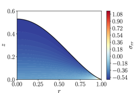
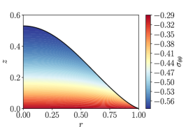
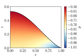
Figure 6: The (a) radial elastic stress, (b) orthoradial elastic stress, and (c) pressure in a dried poroelastic drop with large initial contact angle. The drop has shed half of its volume due to fluid loss ($J=0.50$). We set $\epsilon=0.80$ ($\varphi_{0}\simeq 58^{\circ}$) and $\nu=0.30$.

The stress profiles shown in Fig. 6 indicate that many of the conclusions obtained from the asymptotically reduced model still apply when the contact angle of the drop is not small. However, from Fig. 5, we see that the quantitative accuracy of the asymptotic reduction can only be ensured for drops with initial contact angles that are smaller than $20^{\circ}$.

As a final point, experiments have shown that the drying pathway for colloidal drops with large contact angles involves the formation of an elastic skin at the free surface [1]. Drying-induced stresses lead to buckling of the skin [47] as opposed to fracture. Extending the poroelastic model proposed here to shell-like geometries would allow drying-induced buckling patterns to be studied.

V Concluding remarks

By combining nonlinear poroelasticity with the lubrication approximation, we have derived a simplified model that offers new insights into the generation of mechanical stress during the drying of complex drops. The asymptotic analysis indicates that the initial profile of the solid skeleton $h_{0}$ plays a central role in the poromechanics of drop drying, as it controls the in-plane motion of the solid skeleton. Using the asymptotic solutions for the stress, it is possible to predict the alignment of desiccation fractures.

A limitation of the model proposed here is that is based on the assumption that the drop has a pre-existing poroelastic structure. That is, the model does not consider the regime in which the drop is liquid. As a consequence, the initial profile of the solid skeleton $h_{0}$ must be provided as input to the model. An important area of future work is to develop an extended model that captures the fluid mechanics of drying and the sol-gel transition, with the aim of predicting $h_{0}$. Routh and Russel [48] studied a similar problem but assumed the porous solid was rigid.

When modelling the drying of biological fluids before gelation occurs, non-Newtonian effects may be important to consider. For example, blood is often modelled as a Carreau–Yasuda fluid [49]. In this case, the relevance of non-Newtonian effects can be assessed through the quantity $(\lambda\dot{\gamma})^{a}$, where $\lambda$ is a relaxation time, $\dot{\gamma}$ is the shear rate, and $a$ is a constant. Abraham et al. [50] report that $\lambda=8.2$ s and $a=0.64$ for blood. For a thin drop in the lubrication limit, $\dot{\gamma}\sim U/(\epsilon R)$. Sobac and Brutin [9] state that, before gelation, the fluid velocity $U$ is dominated by capillary action and provide a value of $U=8$ $\mu$m s^-1. Using the parameter values in Sec. II.5 gives $(\lambda\dot{\gamma})^{a}\sim 0.26$, which is small but not negligible. After gelation, the liquid component of blood (mainly water) will flow through a porous network composed of solid biological components (mainly red blood cells). Thus, describing the macroscopic flow field using Darcy’s law, as done here, is appropriate.

With a satisfactory initial profile for the solid skeleton, the asymptotic approach developed here can be extended to a wide range of new problems that capture, for example, delamination, substrate deformability, and fracture. These problems will help to unravel the complex interplay between physical mechanisms that govern the drying of complex fluids and provide a deeper understanding of the various modes of mechanical instability that can occur.