Hybrid Acceleration Scheme for Variance Reduced Stochastic Optimization Algorithms

Abstract

Stochastic variance reduced optimization methods are known to be globally convergent while they suffer from slow local convergence, especially when moderate or high accuracy is needed. To alleviate this problem, we propose an optimization algorithm—which we refer to as a hybrid acceleration scheme—for a class of proximal variance reduced stochastic optimization algorithms. The proposed optimization scheme combines a fast locally convergent algorithm, such as a quasi–Newton method, with a globally convergent variance reduced stochastic algorithm, for instance SAGA or L–SVRG. Our global convergence result of the hybrid acceleration method is based on specific safeguard conditions that need to be satisfied for a step of the locally fast convergent method to be accepted.

We prove that the sequence of the iterates generated by the hybrid acceleration scheme converges almost surely to a solution of the underlying optimization problem. We also provide numerical experiments that show significantly improved convergence of the hybrid acceleration scheme compared to the basic stochastic variance reduced optimization algorithm.

1 Introduction

We consider convex finite–sum optimization problems of the form

$$\underset{x\in\mathbb{R}^{d}}{\text{minimize}}\hskip 5.69054ptF(x)+g(x),$$ (1)

where $F:\mathbb{R}^{d}\to\mathbb{R}$ is the average of convex and smooth functions $f_{i}:\mathbb{R}^{d}\to\mathbb{R}$, that is,

$$F(x)=\tfrac{1}{N}\sum_{i=1}^{N}f_{i}(x),$$

for all $x\in\mathbb{R}^{d}$ and $g:\mathbb{R}^{d}\to\mathbb{R}\cup\{\infty\}$ is a closed, convex, proper, and potentially non–smooth function that can be used as a regularization term or to model convex constraints. Such finite–sum optimization problems are common in machine learning and statistics where they are known as regularized empirical risk minimization problems schmidt2017minimizing (25, 30).

One approach to solve the finite–sum optimization problem (1) is to use the proximal–gradient method beck2009fast (3). However, at each iteration, the proximal–gradient algorithm requires as many individual gradient evaluations as the number of component functions of the finite–sum, which can be computationally expensive. Another approach is to apply stochastic proximal–gradient descent Nitanda2014StochasticPG (17, 23), which requires only one gradient evaluation at each iteration, but, due to the variance in the estimation of the full gradient, suffers from sub–linear convergence rate, even in the strongly convex setting johnson2013accelerating (11, 12). Several stochastic variance–reduced optimization algorithms such as SDCA shalev2013stochastic (28), SVRG johnson2013accelerating (11), and SAGA defazio2014saga (8), have been designed to reduce the gradient approximation variance. These methods have been shown to be practically efficient and achieve global (linear) convergence for (strongly) convex problems. However, their local convergence is often slow in practice.

To improve convergence, pre–determined data preconditioning li2017preconditioned (13, 33) or metric selection giselsson2015metric (9) can be used. These are generic approaches that can be applied on top of acceleration schemes. However, finding the optimal or even a good metric is problem– and algorithm–dependent and might be computationally expensive. Quasi–Newton type methods, such as Anderson acceleration Anderson1965IterativePF (1, 32) and limited–memory BFGS liu1989limited (14), instead find a suitable metric on the fly. Compared to stochastic optimization algorithms, these methods have higher per–iteration cost, but, often exhibit very fast local convergence. However, global convergence results are scarce for non–smooth problems, whereas some results exist for fully smooth problems Rodomanov2021GreedyQM (20, 21, 22).

In this paper, we provide a generic algorithm that combines a method with locally fast convergence (that will be called acceleration method) with a globally convergent proximal stochastic optimization algorithm (that will be called basic method). The key feature of the general algorithm is a set of safeguard conditions that decide if an acceleration step can be accepted while maintaining global convergence. If the safeguard conditions are not satisfied, a step of the basic method is taken. This results in a hybrid scheme that automatically selects between two different algorithms and benefits both from the global convergence properties of the basic method and the fast local convergence of the acceleration method. We refer to our proposed algorithm as the hybrid acceleration scheme.

The idea of a hybrid algorithm that selects between a globally convergent method and locally fast, but not globally, convergent method has been explored, e.g., in themelis2019supermann (31, 34), whose selection criteria are extensions of the one in giselsson2016line (10). A key difference between our approach and themelis2019supermann (31, 34) is that their methods are based on a deterministic basic method, while ours is based on a variance reduced stochastic method. This difference necessitates a completely different convergence analysis and enables for faster progress far from the solution in our finite–sum problem setting since our method takes advantage of that particular problem structure schmidt2017minimizing (25).

Due to the flexibility of our scheme, many different locally fast methods can be used. For instance; limited–memory BFGS (lBFGS) liu1989limited (14), Anderson acceleration Anderson1965IterativePF (1), and the class of vector extrapolation methods smith1987extrapolation (29) to which, e.g., the regularized nonlinear acceleration scieur2016regularized (27) and its stochastic counterpart scieur2017nonlinear (26) belong.

We instantiate our hybrid method with two different local methods, namely limited–memory BFGS (lBFGS) liu1989limited (14) and Anderson acceleration Anderson1965IterativePF (1). In our numerical experiments, we combine these methods with Loop–less SVRG kovalev2019don (12) in our hybrid acceleration method. Our numerical experiments show that our hybrid acceleration scheme can exhibit significantly improved convergence compared to the basic stochastic optimization algorithm.

The paper is outlined as follows. In Section 2, we recall some basic definitions. Section 3 discusses the problem formulation and the link between deterministic and stochastic gradient methods and introduces the family of stochastic optimization algorithms that is considered in this work. In Section 4, the hybrid acceleration method is introduced and in Section 5, we prove its convergence. Numerical experiments are presented in Section 6 and concluding remarks are given in Section 7.

2 Preliminaries

The set of the real numbers and the $d$-dimensional Euclidean space are denoted by $\mathbb{R}$ and $\mathbb{R}^{d}$ respectively. For a symmetric positive definite matrix $\Gamma$ and $x,y\in\mathbb{R}^{d}$, $\langle x,y\rangle$, $\|x\|$, and $\|x\|_{\Gamma}$ are the inner product, the induced norm, and the weighted norm $\|x\|_{\Gamma}:=\sqrt{\langle x,\Gamma x\rangle}$ respectively. Moreover, the $d\times d$ identity matrix is denoted by $I_{d}$.

The notation $2^{\mathbb{R}^{d}}$ denotes the power set of $\mathbb{R}^{d}$. A map $A:\mathbb{R}^{d}\rightrightarrows 2^{\mathbb{R}^{d}}$ is characterized by its graph $\operatorname{gra}(A)=\{(x,u)\in\mathbb{R}^{d}\times\mathbb{R}^{d}:u\in Ax\}$. The operator $A$ is monotone, if $\mathord{\left\langle u-v,x-y\right\rangle}\geq 0$ for all $(x,u),(y,v)\in\operatorname{gra}(A)$. A monotone operator $A$ is maximally monotone if there exists no monotone operator $B:\mathbb{R}^{d}\rightrightarrows 2^{\mathbb{R}^{d}}$ such that $\operatorname{gra}(B)$ properly contains $\operatorname{gra}(A)$. A mapping $T:\mathbb{R}^{d}\rightarrow\mathbb{R}^{d}$ is $L$-Lipschitz continuous if $\|T(x)-T(y)\|\leq L\|x-y\|$ for all $x,y\in\mathbb{R}^{d}$, and is nonexpansive if it is 1-Lipschitz continuous. Further $T:\mathbb{R}^{d}\rightarrow\mathbb{R}^{d}$ is

1. firmly nonexpansive if

   $$\|x-y-(T(x)-T(y))\|^{2}\leq\|x-y\|^{2}-\|T(x)-T(y)\|^{2}\quad\quad\forall x,y\in\mathbb{R}^{d},$$

2. $\tfrac{1}{L}$-cocoercive if

   $$\langle T(x)-T(y),x-y\rangle\geq\tfrac{1}{L}\|T(x)-T(y)\|^{2}\quad\quad\forall x,y\in\mathbb{R}^{d}.$$

For a mapping $T$, $\tfrac{1}{L}$-cocoercivity implies its $L$-Lipschitz continuity. The other direction does not hold in general. However, if the mapping is the gradient of a convex function, then its $L$-Lipschitz continuity and $\tfrac{1}{L}$-cocoercivity are equivalent (bauschke2017convex, 2, Corollary 18.17). A differentiable function $F:\mathbb{R}^{d}\rightarrow\mathbb{R}$ is said to be $L$-smooth, if its gradient is $L$-Lipschitz continuous.

The subdifferential of a function $f:\mathbb{R}^{d}\rightarrow\mathbb{R}\cup\{\infty\}$ at $x\in\mathbb{R}^{d}$ is denoted by $\partial f(x)$ and defined as

$$\partial f(x)=\{v\in\mathbb{R}^{d}:f(y)\geq f(x)+\mathord{\left\langle v,y-x\right\rangle}\text{~{}for all~{}}y\in\mathbb{R}^{d}\}.$$

The proximal mapping of a closed, convex and proper function $g:\mathbb{R}^{d}\rightarrow\mathbb{R}\cup\{+\infty\}$, is defined as $\operatorname{prox}_{\lambda g}(v)=\underset{x}{\mathrm{argmin}}\left(g(x)+\tfrac{1}{2\lambda}\|x-v\|^{2}\right)$, where $\lambda>0$.

The set of fixed–points of a mapping $\mathcal{T}:\mathbb{R}^{d}\rightarrow\mathbb{R}^{d}$, is denoted by $\mathrm{fix}\mathcal{T}$ and defined as $\mathrm{fix}\mathcal{T}=\{x\in\mathbb{R}^{d}:x=\mathcal{T}x\}$. The zero–set of a map ${\mathcal{R}}:\mathbb{R}^{d}\rightarrow\mathbb{R}^{d}$ is indicated by $\mathrm{zer}{\mathcal{R}}$ and given by $\mathrm{zer}{\mathcal{R}}=\{x\in\mathbb{R}^{d}:0={\mathcal{R}}x\}$. It is evident that $\mathrm{fix}\mathcal{T}=\mathrm{zer}{(\mathrm{Id}-\mathcal{T})}$, where $\mathrm{Id}-\mathcal{T}$ is the residual map of the operator $\mathcal{T}$.

3 Problem formulation and basic method

We are interested in solving the following convex optimization problem

$$\underset{x\in\mathbb{R}^{d}}{\text{minimize}}\hskip 5.69054pt\tfrac{1}{N}\sum_{i=1}^{N}f_{i}(x)+g(x),$$ (2)

under the following assumptions.

Assumption 3.1

We assume that

1. For each $i\in\{1,\ldots,N\}$, the function $f_{i}:\mathbb{R}^{d}\rightarrow\mathbb{R}$ is convex, differentiable and $L_{i}$-smooth.

2. The function $g:\mathbb{R}^{d}\rightarrow\mathbb{R}\cup\{+\infty\}$ is convex, closed and proper.

3. The solution set of the problem is nonempty.

The necessary and sufficient optimality condition for this problem is given by Fermat’s rule as

$$0\in{\partial(F+g)(x)=}\mathrm{\nabla}F(x)+\partial g(x){,}$$ (3)

where the equality holds since all $f_{i}$ have full domain and $g$ is proper (bauschke2017convex, 2, Theorem 16.3 and Corollary 16.48). This means that any $x^{\star}$ that satisfies the optimality condition (3), is a solution to the associated optimization problem (2). It is also known that fixed–points of the proximal–gradient operator, namely, the set $\{x\in\mathbb{R}^{d}:x=\operatorname{prox}_{\lambda g}(x-\lambda\nabla F(x)),\lambda>0\}$, are solutions of problem (2). In fact, all solutions of the inclusion problem (3), are fixed–points of the proximal–gradient operator or, equivalently, zeros of its residual mapping, which is given by

$${\mathcal{R}}x=x-\operatorname{prox}_{\lambda g}\left(x-\lambda\nabla F(x)\right),$$

for any $\lambda>0$ (parikh2014proximal, 19, Section 4.2). For $0<\lambda<\tfrac{2}{L}$ with $L$ being the smoothness modulus of $F$, iterating the proximal gradient mapping finds a solution of problem (2) combettes2011proximal (5).

The optimality condition (3), can be reformulated in a primal–dual form by storing all gradients of component functions $f_{i}$. In that case, the optimality condition becomes

$$\begin{cases}&0\in\partial g(x)+\tfrac{1}{N}\sum_{i=1}^{N}y_{i}\\ &0=y_{1}-\mathrm{\nabla}f_{1}(x)\\ &\quad\vdots\\ &0=y_{N}-\mathrm{\nabla}f_{N}(x)\end{cases},$$ (4)

where $y_{i}$ denotes the $i$–th dual variable. This is clearly equivalent to (3). Therefore, a primal–dual solution $z^{\star}:=(x^{\star},y_{1}^{\star},\ldots,y_{N}^{\star})$ satisfies (4), if and only if $x^{\star}$ satisfies (3) and is a solution of (2). It also holds that $z^{\star}$ satisfies (4) if and only if it satisfies $\bar{\mathcal{R}}z^{\star}=0$, where $\bar{\mathcal{R}}$ is the primal–dual residual mapping

$$\bar{\mathcal{R}}z:=\begin{pmatrix}x-\operatorname{prox}_{\lambda g}\left(x-\tfrac{\lambda}{N}\sum_{i=1}^{N}y_{i}\right)\\ y_{1}-\mathrm{\nabla}f_{1}(x)\\ \vdots\\ y_{N}-\mathrm{\nabla}f_{N}(x)\end{pmatrix},$$ (5)

in which $z=(x,y_{1},\ldots,y_{N})$ is the primal–dual variable. We record the equivalence between zeroes of $\bar{\mathcal{R}}$ and solutions to (2), in Proposition 1 (with proof in Appendix A.1) and Lipschitz continuity of $\bar{\mathcal{R}}$ in Proposition 2 (with proof in Appendix A.2).

Proposition 1

Given the residual map in (5), the primal–dual point $z^{\star}=(x^{\star},y_{1}^{\star},\ldots,y_{N}^{\star})$ satisfies $\bar{\mathcal{R}}z^{\star}=0$, if and only if $x^{\star}$ solves (2). Furthermore, for each index $i$, $y_{i}^{\star}$ is unique.

Proposition 2

Let for all $i\in\{1,\ldots,N\}$, $f_{i}(x)$ be $L_{i}$-smooth, then the primal–dual residual mapping, $\bar{\mathcal{R}}$ in (5), is Lipschitz-continuous.

In order to find zeros of $\bar{\mathcal{R}}$, one way is to form iterates based on (5), and evaluate all $y_{i}$’s (the full gradient) at each iteration, which would be similar to the proximal–gradient algorithm. However, when $N$ is very large, a key challenge is the high per–iteration cost of $N$ gradient evaluations which makes the algorithm very expensive. This gives rise to the idea of using a cheaply evaluable approximation of the true gradient instead, and randomly evaluate gradients of only one or some of $f_{i}$’s at each iteration. The following gives such an approximation

$$\widehat{\nabla}_{i_{k}}F(x,y)\triangleq\tfrac{1}{Np_{i_{k}}}\left(\mathrm{\nabla}f_{i_{k}}(x)-y_{i_{k}}\right)+\tfrac{1}{N}\sum\limits_{i=1}^{N}y_{i},$$ (6)

in which $i_{k}$ is an index randomly drawn from $\{1,\ldots,N\}$ based on some probability distribution and $p_{i_{k}}$ is its associated probability. This stochastic approximation is based on the average of the dual variables which is modified by a correction term, $(\mathrm{\nabla}f_{i_{k}}(x)-y_{i_{k}})/({Np_{i_{k}}})$. The correction term is added in order to progressively improve the approximation by incorporating the latest gradient information and also to make $\widehat{\nabla}_{i_{k}}F(x,y)$ an unbiased estimate of the true gradient.

Using the approximation $\mathrm{\nabla}F(x)\approx\widehat{\nabla}_{i_{k}}F(x,y)$, and inspired by the proximal gradient algorithm, a family of proximal stochastic optimization algorithms can be formulated as

$$x^{k+1} =\operatorname{prox}_{\lambda g}\left(x^{k}-\lambda\widehat{\nabla}_{i_{k}}F(x^{k},y^{k})\right),$$ (7)

$$y_{i}^{k+1} =y_{i}^{k}+\varepsilon_{i}^{k}(\mathrm{\nabla}f_{i}(x^{k})-y_{i}^{k}),\quad\forall i\in\{1,\ldots,N\},$$

where $k$ is the iteration counter, $x^{k}$ is the primal variable, $y^{k}=(y_{1}^{k},\ldots,y_{N}^{k})$ with $y_{i}^{k}$ being the $i$–th dual variable, $\lambda>0$ is the step size, $\varepsilon_{i}^{k}{\in\{0,1\}}$ is a random binary variable that determines whether the $i$–th dual variable is to be updated at iteration $k$ (the associated probability of $\varepsilon_{i}^{k}=1$ is $\rho_{i}$), and $\widehat{\nabla}_{i_{k}}F(x^{k},y^{k})$ is the stochastic approximation of the true gradient that is defined in (6). This approximation of the full gradient is unbiased since

$$\operatorname{\mathbb{E}}_{k}(\widehat{\nabla}_{i_{k}}F(x^{k},y^{k})) =\tfrac{1}{N}\sum_{i=1}^{N}(\mathrm{\nabla}f_{i}(x^{k})-y_{i}^{k})+\tfrac{1}{N}\sum_{i=1}^{N}y_{i}^{k}$$

$$=\tfrac{1}{N}\sum_{i=1}^{N}\mathrm{\nabla}f_{i}(x^{k})=\mathrm{\nabla}F(x^{k}){,}$$

in which, $\operatorname{\mathbb{E}}_{k}$ denotes expected value operation given all available information up to step $k$. We refer to (7) as the basic method. On the other hand, there are algorithms that use a biased estimation of the true gradient morin2019svag (16, 24), but in this work we only consider the unbiased case. The algorithm in (7) has been analyzed in davis2016smart (7) in the monotone operator setting and in morin2020sampling (15) in the strongly convex setting.

The class of stochastic optimization algorithms (7) has L–SVRG davis2016smart (7, 12) and SAGA defazio2014saga (8) as special cases. The L–SVRG algorithm is extracted from (7) with uniform sampling of $i_{k}\in\{1,\ldots,N\}$ and

$$\varepsilon_{i}^{k}=\begin{cases}1\qquad\mathrm{if}\hskip 2.84526ptq<\rho\\ 0\qquad\mathrm{otherwise}\end{cases},\quad\forall i\in\{1,\ldots,N\},$$

where $q$ is uniformly sampled from $[0,1]$ and $0<\rho\leq 1$. Therefore, all dual variables are updated together and on average once every $\rho^{-1}$ iterations. The algorithm in (7) reduces to SAGA with $i_{k}$ uniformly sampled from $\{1,\ldots,N\}$ and

$$\varepsilon_{i}^{k}=\begin{cases}1\qquad\mathrm{if}\hskip 2.84526pti_{k}=i\\ 0\qquad\mathrm{otherwise}\end{cases},\quad\forall i\in\{1,\ldots,N\}.$$

Therefore, for SAGA, at each iteration, only one of the dual variables is updated and the others remain unchanged.

4 Hybrid acceleration scheme

In this section, we introduce a novel hybrid strategy to accelerate local convergence of proximal stochastic optimization algorithms of the form (7), in which the approximation of the true gradient and the update law of the dual variables, vary depending on the choice of basic method. The basic method (7), is devised to solve large–scale finite–sum optimization problems of the form (2), and is globally convergent while it has slow local convergence. Therefore, in our acceleration scheme, they are combined with a locally fast convergent method. The proposed acceleration scheme is given in Algorithm 1 and discussed below.

Algorithm 1   General framework of the hybrid acceleration scheme

1:Input: initial point $z^{0}$, positive constants $C$, $D$, $\delta$, merit function $V(.)$, acceleration algorithm $\mathcal{A}(.)$ and its memory size $m$ (if needed), $K_{0}$, the basic method and its parameters, primal and dual probability distribution, the step size $\lambda$, $\Gamma=\mathrm{blkdiag}(I_{d},\tfrac{\lambda}{N\rho_{1}L_{1}}I_{d},\ldots,\tfrac{\lambda}{N\rho_{N}L_{N}}I_{d})$, and the maximum permissible number of iterations $k_{max}$.

2:set $k=k_{\mathrm{aa}}=0$

3:while $k<k_{max}$ do

4:     $m_{k_{\mathrm{aa}}}=\min\{m,k_{\mathrm{aa}}\}$

5:     find $z^{+}=\mathcal{A}(z^{k},z^{{k_{\mathrm{aa}}-1}},\ldots,z^{{k_{\mathrm{aa}}-m_{k_{\mathrm{aa}}}}})$ from acceleration algorithm

6:     if $V(z^{+})\leq\frac{CV(z^{0})}{(k_{\mathrm{aa}}+1)^{(1+\delta)}}$ and $\left\|z^{+}-z^{k}\right\|_{\Gamma}\leq DV(z^{k})$ then

7:         set $z^{k+1}=z^{+}$ and $k_{\mathrm{aa}}\leftarrow k_{\mathrm{aa}}+1$

8:         $k\leftarrow k+1$ and $k_{\mathrm{aa}}\leftarrow k_{\mathrm{aa}}+1$

9:     else

10:         set $(\widetilde{x}^{0},\widetilde{y}_{1}^{0},\ldots,\widetilde{y}_{N}^{0})=z^{k}$

11:         for $s=0,1,\cdots,K_{0}-1$ do

$$\begin{cases}\widetilde{x}^{s+1}=\operatorname{prox}_{\lambda g}\left(\widetilde{x}^{s}-\lambda\widehat{\nabla}_{i_{s}}F(\widetilde{x}^{s},\widetilde{y}^{s})\right),\\ \widetilde{y}_{i}^{s+1}=\widetilde{y}_{i}^{s}+\varepsilon_{i}^{s}(\mathrm{\nabla}f_{i}(\widetilde{x}^{s})-\widetilde{y}_{i}^{s}),\quad\forall i\in\{1,\ldots,N\}.\end{cases}$$

$$\hskip 7.96677ptz^{k+1}=(\widetilde{x}^{s+1},\widetilde{y}_{1}^{s+1},\ldots,\widetilde{y}_{N}^{s+1})$$

$$\hskip 7.96677ptk\leftarrow k+1$$

12:         end for

13:     end if

14:end while

Description of the algorithm.

In order to initialize the scheme one needs to select (i) the parameters and probability distributions used in the basic method; (ii) an acceleration algorithm $\mathcal{A}(.)$ along with its associated parameters; and (iii) an initial point $z^{0}$. The acceleration algorithm $\mathcal{A}(.)$ can be algorithms such as lBFGS or Anderson acceleration that both store and use a history of past $m$ iterates to find a next iterate. Then, the algorithm works as follows: at the beginning of each iteration the iterate from the acceleration algorithm, $z^{+}$, has to be computed. If $z^{+}$ satisfies some safeguard conditions, that we will discuss below, we set it as the true next iterate, $z^{k+1}$, and the main counter of the loop, $k$, and also the acceleration algorithm’s counter, $k_{aa}$, are increased by one; then, we proceed to the next iteration. Otherwise, $K_{0}$ steps of the basic method are performed in the inner loop of the algorithm. It is evident that $K_{0}$ can differ among different iterations of the outer loop of the scheme, but, we considered it as a constant for simplicity. The algorithm is to be run as above until the last iteration is reached or some termination criteria are met. Note that if the iterate from the acceleration algorithm is accepted, the basic method steps need not to be performed, that is, the basic method and the acceleration algorithm are not being run in parallel.

Safeguard conditions and merit function.

For a nominal next iterate of the acceleration algorithm, $z^{+}$, to be accepted as the actual next iterate of the scheme, the following conditions have to be satisfied

$$V(z^{+}) \leq CV(z^{0})(1+k_{\mathrm{aa}})^{-(1+\delta)},$$ (8)

$$\left\|z^{+}-z^{k}\right\|_{\Gamma} \leq DV(z^{k}),$$ (9)

where $\delta$, $C$ and $D$ are positive constants, $V:\mathbb{R}^{(N+1)d}\rightarrow\mathbb{R}$ is a merit function (that is discussed below), and

$$\Gamma=\mathrm{blkdiag}(I_{d},\tfrac{\lambda}{N\rho_{1}L_{1}}I_{d},\ldots,\tfrac{\lambda}{N\rho_{N}L_{N}}I_{d}).$$

The safeguard condition (8) enforces the merit function to be convergent to zero. Condition (9), is to ensure that the sequence $(\|z^{k+1}-z^{k}\|_{\Gamma})_{k\in I_{\mathrm{aa}}}$, where $I_{\mathrm{aa}}$ is the set of indices for which the next iterate is obtained from acceleration algorithm, is diminishing and finally convergent to zero.

Our convergence theory, that will be given in the next section, assumes that; i) the merit function outputs nonnegative values, ii) for any sequence $(z^{k})_{k\in\mathbb{N}}$, the merit function is such that

$$V(z^{k})\to 0\qquad\Longrightarrow\qquad\left\|\bar{\mathcal{R}}z^{k}\right\|\to 0.$$

Therefore, a feasible choice for the merit function can be the following scaled $l_{2}$–norm of $\bar{\mathcal{R}}z^{k}$

$$V(z^{k})=\left\|\bar{\mathcal{R}}z^{k}\right\|_{\Gamma}.$$ (10)

For this choice of merit function, which we use in this work, both requirements on the merit function are met. Other options for the merit function could be the sum or maximum of the vector of the last $p$ scaled $l_{2}$–norm of residuals.

5 Convergence results

In this section, we provide results on convergence of the basic method and the hybrid acceleration scheme. Before proceeding to convergence results, we summarize the notations and the assumptions that are used in the theorems and their proofs. The proofs are given in the Appendix.

Notation.

$\mathcal{X}^{\star}$ indicates the solution set of problem (2), $z=(x,y_{1},\ldots,y_{N})$ denotes a primal–dual variable for (5), $\bar{\mathcal{R}}$ is the primal–dual residual operator defined in (5), $z^{\star}=(x^{\star},y_{1}^{\star},\ldots,y_{N}^{\star})$ is an arbitrary point in the set of zeros of the primal–dual residual mapping with $y_{i}^{\star}=\mathrm{\nabla}f_{i}(x^{\star})$, $p_{i}$ is primal sampling probability, $\rho_{i}$ is the $i$–th dual variable update probability, $\lambda>0$ is the step size, $\operatorname{\mathbb{E}}_{k}$ denotes the expected value operator given all the information up to the $k$–th iteration, and $\Gamma=\mathrm{blkdiag}(I_{d},\tfrac{\lambda}{N\rho_{1}L_{1}}I_{d},\ldots,\tfrac{\lambda}{N\rho_{N}L_{N}}I_{d})$. Moreover, $z^{k}=(x^{k},y_{1}^{k},\ldots,y_{N}^{k})$ denotes the $k$–th primal–dual iterate; and $(z^{k})_{k\in\mathbb{N}}$, $(x^{k})_{k\in\mathbb{N}}$, and $(y_{i}^{k})_{k\in\mathbb{N}}$ are the sequences of primal–dual-, primal-, and the $i$–th dual iterates, respectively.

The following is a result that is used in proof of Theorem 5.2. The proof can be found in Appendix A.3.

Proposition 3

Under Assumption 3.1, almost sure (a.s.) convergence of $(z^{k})_{k\in\mathbb{N}}$ to a $\bar{z}\in\mathrm{zer}{\bar{\mathcal{R}}}$, implies a.s. convergence of $(x^{k})_{k\in\mathbb{N}}$ and $(y_{i}^{k})_{k\in\mathbb{N}}$ to a $\bar{x}\in\mathcal{X}^{\star}$ and $\bar{y}_{i}=\mathrm{\nabla}f_{i}(\bar{x})$ respectively.

The result in Theorem 5.1 and its proof (given in Appendix A.5) share similarities with davis2016smart (7, 15).

Theorem 5.1

Let $z^{k}$ be the $k$–th primal–dual iterate associated with the basic method iterates in (7), then given Assumption 3.1, the following holds

$$\operatorname{\mathbb{E}}_{k}\|z^{k+1}-z^{\star}\|_{\Gamma}^{2}\leq\|z^{k}-z^{\star}\|_{\Gamma}^{2}-\zeta_{k},$$

with

$$\zeta_{k} =\sum_{i=1}^{N}\tfrac{\lambda}{N}(\tfrac{1}{L_{i}}-\tfrac{2\lambda}{Np_{i}})\left(\|\mathrm{\nabla}f_{i}(x^{k})-\mathrm{\nabla}f_{i}(x^{\star})\|^{2}+\|y_{i}^{k}-y_{i}^{\star}\|^{2}\right)$$ (11)

$$\qquad+\tfrac{2\lambda^{2}}{N^{2}}\|\sum_{i=1}^{N}(y_{i}^{k}-y_{i}^{\star})\|^{2}+\lambda^{2}\|\mathrm{\nabla}F(x^{k})-\mathrm{\nabla}F(x^{\star})\|^{2}$$

$$\qquad+\operatorname{\mathbb{E}}_{k}\|x^{k+1}-x^{k}+\lambda(\widehat{\nabla}_{i_{k}}F(x^{k},y^{k})-\mathrm{\nabla}F(x^{\star}))\|^{2}.$$

Furthermore, if $0<\lambda<\mathrm{min}_{i}\{\tfrac{Np_{i}}{2L_{i}}\}$, then $(z^{k})_{k\in\mathbb{N}}$ converges a.s. to a random variable $\bar{z}\in\mathrm{zer}{\bar{\mathcal{R}}}$ and $(x^{k})_{k\in\mathbb{N}}$ and $(y_{i}^{k})_{k\in\mathbb{N}}$ converge a.s. to random variables $\bar{x}\in\mathcal{X}^{\star}$ and $\bar{y}_{i}=\mathrm{\nabla}f_{i}(\bar{x})$ respectively.

Remark 1

In order to ensure a.s. convergence in Theorem 5.1, the coefficient of all terms in $\zeta_{k}$ must be positive. Then, from relation (11), it is evident that for each $i$, $0<\lambda<\tfrac{Np_{i}}{2L_{i}}$ must hold. Therefore, the smallest of these has to be set as the upper bound of $\lambda$, that is, $0<\lambda<\mathrm{min}_{i}\{\tfrac{Np_{i}}{2L_{i}}\}$. The largest upper bound of the step size is attained when we have Lipschitz probability distribution for primal sampling, namely, $p_{i}=\tfrac{L_{i}}{\sum_{i=1}^{N}L_{i}}$.

The following result is on a.s. convergence of the sequence of iterates that are obtained from Algorithm 1. The proof is presented in Appendix A.6.

Theorem 5.2

Suppose that Assumption 3.1 holds, that $0<\lambda<\mathrm{min}_{i}\{\tfrac{Np_{i}}{2L_{i}}\}$, and that the merit function $V:\mathbb{R}^{(N+1)d}\to\mathbb{R}$ is nonnegative and such that for all sequences $(z^{k})_{k\in\mathbb{N}}$ satisfying $V(z^{k})\to 0$ we have $\|\bar{\mathcal{R}}z^{k}\|\to 0$. Then $(z^{k})_{k\in\mathbb{N}}$ in Algorithm 1 converges a.s. to a random variable $\bar{z}\in\mathrm{zer}{\bar{\mathcal{R}}}$. Moreover, $(x^{k})_{k\in\mathbb{N}}$ and $(y_{i}^{k})_{k\in\mathbb{N}}$ converge a.s. to random variables $\bar{x}\in\mathcal{X}^{\star}$ and $\bar{y}_{i}=\mathrm{\nabla}f_{i}(\bar{x})$ respectively.

6 Numerical experiments

We solve a regularized logistic regression problem for binary classification of the form

$$\underset{x=(w,b)}{\text{minimize}}\hskip 5.69054pt\sum_{i=1}^{N}{\text{log}(1+e^{\theta_{i}^{T}w+b})-u_{i}(\theta_{i}^{T}w+b)}+\tfrac{\xi}{2}\|w\|_{2}^{2},$$ (12)

where $\theta_{i}\in\mathbb{R}^{d}$ and $u_{i}\in\{0,1\}$ are training data and labels respectively, and $\xi>0$ is a regularization parameter. The optimization problem variable is $x=(w,b)$ with $w\in\mathbb{R}^{d}$ and $b\in\mathbb{R}$.

In the hybrid acceleration scheme, we use L–SVRG as the basic method and either Anderson acceleration or lBFGS as the acceleration algorithms. The following lists the algorithms that are used in the numerical experiments

• GD: Gradient descent method with fixed step size,

• L–SVRG: Loopless Stochastic Variance Reduced Gradient method,

• L–SVRG+AA: L–SVRG as the basic method combined with Anderson acceleration,

• L–SVRG+lBFGS: L–SVRG as the basic method combined with limited–memory BFGS.

In order to use Anderson acceleration as the acceleration algorithm in the hybrid acceleration scheme, an associated fixed–point mapping of problem (12) is needed. Let $F(x)$ denote the objective function of problem (12). Then, the associated mapping of the problem that is used by Anderson acceleration is given by

$$\mathcal{T}_{gd}(x)=x-\lambda\nabla F(x)$$

for $\lambda\in(0,2/L)$, where $L$ is smoothness modulus of $F$. On the other hand, since the objective function at hand has no non–smooth part, the lBFGS algorithm can also be utilized in the hybrid acceleration scheme to solve problem (12). Unlike Anderson acceleration, lBFGS method does not need an associated fixed–point map of the problem, rather, it requires gradients of the objective function in order to find a solution. See Appendix B.1 and Appendix B.2 for descriptions of Anderson acceleration and lBFGS methods, respectively.

A rough approximation of the per–iteration count of floating point operations for the different algorithms are as follows

• $4Nd$ for gradient descent,

• $12Nd$ for L–SVRG,

• $4Nd+\tfrac{4}{3}m^{3}+2m^{2}d$ for Anderson acceleration,

• $4Nd+2d^{2}+13md+\xi_{bt}4Nd$ for lBFGS,

where, $N$ is the number of the component functions (which is the same as the number of samples in the training dataset), $d$ is the dimension of the optimization problem variable, $m$ is the size of memory stack for either Anderson acceleration or lBFGS and $\xi_{bt}$ is a coefficient to include an approximate average cost for back-tracking line search of lBFGS.

Numerical simulations are done using two datasets; UCI Madelon CC01a (4) with 2000 samples and 500 features, and UCI Sonar CC01a (4) with 208 samples and 60 features. In the numerical experiments, the regularization parameter in the objective function is set to $\xi=0.01$, we used a memory size of $m=5$ for both Anderson acceleration and lBFGS, the constants of the safeguard condition of the hybrid acceleration scheme is $C=D=10^{6}$, and $\delta=10^{-6}$, and the parameter $K_{0}$ is set to the number of samples of the associated dataset. Moreover, we used the merit function as is defined in (10).

In Figure 1 and Figure 2, the left plots show relative value of objective function versus step number (which is basically equal to the total number of full gradient evaluations up to that step), and the right plot illustrates the relative value of objective function versus weighted iteration counts. The weighted iteration is intended to include a rough approximation of computational cost in such a way that different methods at each weighted iteration have roughly the same computational expense. Therefore, it provides a better comparison in terms of computational complexity among different algorithms. The simulation results show remarkable improvement in convergence rate and overall computational cost of the hybrid acceleration scheme compared to those of the basic method.

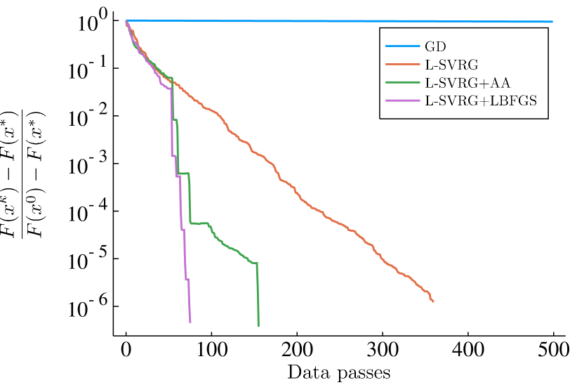
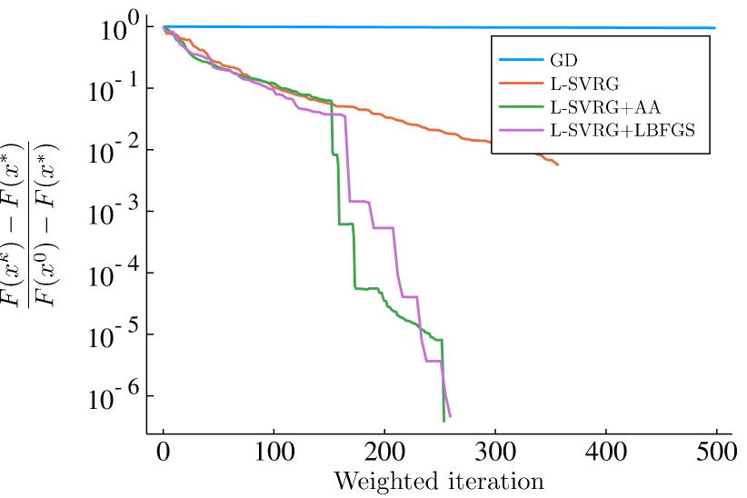
Figure 1: Normalized sub-optimality vs. number of passes over data (the plot to the left) and weighted iteration number (the plot to the right) for the logistic regression problem (12), on UCI Madelon dataset (2000 samples, 500 features), solved using GD, L–SVRG, L–SVRG+AA and L–SVRG+lBFGS methods with regularization parameter $\xi=0.01$.

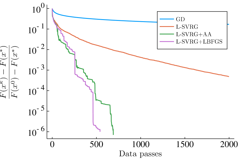
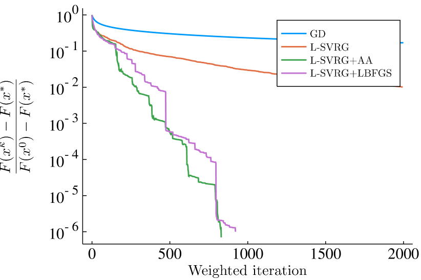
Figure 2: Normalized sub-optimality vs. number of passes over data (the plot to the left) and weighted iteration number (the plot to the right) for the logistic regression problem (12), on UCI Sonar dataset (208 samples, 60 features), solved using GD, L–SVRG, L–SVRG+AA and L–SVRG+lBFGS methods with regularization parameter $\xi=0.01$.

7 Conclusion

In this paper, we proposed and showed almost sure convergence of a hybrid acceleration scheme. It combines a globally convergent variance reduced stochastic gradient method—the basic method—with a fast locally convergent method—the acceleration method—to benefit from the strengths of both methods; global convergence of the basic method and fast local convergence of the acceleration method. Our numerical experiments show that our algorithm performs significantly better than the basic method in isolation, while preserving global convergence guarantees that the local acceleration methods lack.

Appendix A

In what follows, we provide the proofs of the propositions and the theorems that are not addressed in the body of the paper.

A.1 Proof of Proposition 1

From $\bar{\mathcal{R}}z^{\star}=0$ and for any $\lambda>0$ we have

$$\begin{cases}x^{\star}-\operatorname{prox}_{\lambda g}\left(x^{\star}-\tfrac{\lambda}{N}\sum_{i=1}^{N}y_{i}^{\star}\right)=0\\ y_{1}^{\star}=\mathrm{\nabla}f_{1}(x^{\star})\\ \qquad\vdots\\ y_{N}^{\star}=\mathrm{\nabla}f_{N}(x^{\star})\end{cases} \quad\iff\quad x^{\star}-\operatorname{prox}_{\lambda g}\left(x^{\star}-\lambda\nabla F(x^{\star})\right)=0$$

$$\quad\iff\quad 0\in\nabla F(x^{\star})+\partial g(x^{\star})$$

$$\quad\iff\quad 0\in\partial(F+g)(x^{\star}),$$

where the last equivalence holds due to $f_{i}$’s and $g$ having full domain (bauschke2017convex, 2, Theorem 16.3 and Corollary 16.48). Therefore, by Fermat’s rule $x^{\star}$ is a solution of problem (2).

Now suppose that ${x}_{1}^{\star}$ and ${x}_{2}^{\star}$ are two distinct solutions to the problem, that is

$$-\nabla F({x}_{1}^{\star}) \in\partial g({x}_{1}^{\star}),$$

$$-\nabla F({x}_{2}^{\star}) \in\partial g({x}_{2}^{\star}).$$

Then using the fact that $\partial g$ is monotone and that each $\nabla f_{i}$ is $\tfrac{1}{L_{i}}$-cocoercive, we have

$$0\geq\left\langle{x}_{2}^{\star}-{x}_{1}^{\star},\mathrm{\nabla}F\left({x}_{2}^{\star}\right)-\mathrm{\nabla}F\left({x}_{1}^{\star}\right)\right\rangle\geq\sum_{i=1}^{N}\tfrac{1}{NL_{i}}\left\|\mathrm{\nabla}f_{i}({x}_{2}^{\star})-\mathrm{\nabla}f_{i}({x}_{1}^{\star})\right\|^{2}\geq 0,$$

which gives that ${y}_{i}^{\star}=\mathrm{\nabla}f_{i}({x}_{2}^{\star})=\mathrm{\nabla}f_{i}({x}_{1}^{\star})$ for all $i$’s. Hence it follows that ${y}_{i}^{\star}=\mathrm{\nabla}f_{i}({x}^{\star})$ is unique. ∎

A.2 Proof of Proposition 2

In the following proof, we use nonexpansiveness of the proximal operator and $L_{i}$-Lipschitz continuity of $\mathrm{\nabla}f_{i}(x)$ for all $i$

$$\mathord{\left\|\bar{\mathcal{R}}\hat{z}-\bar{\mathcal{R}}z\right\|}^{2} =\mathord{\left\|\hat{x}-\operatorname{prox}_{\lambda g}\bigg{(}\hat{x}-\tfrac{\lambda}{N}\sum_{i=1}^{N}{\hat{y}_{i}}\bigg{)}-x+\operatorname{prox}_{\lambda g}\bigg{(}x-\tfrac{\lambda}{N}\sum_{i=1}^{N}{y_{i}}\bigg{)}\right\|}^{2}$$

$$\qquad+\sum_{i=1}^{N}{\mathord{\left\|\hat{y}_{i}-\mathrm{\nabla}f_{i}(\hat{x})-y_{i}+\mathrm{\nabla}f_{i}(x)\right\|}}^{2}$$

$$\leq\Bigg{(}\mathord{\left\|\hat{x}-x\right\|}+\mathord{\left\|\hat{x}-\tfrac{\lambda}{N}\sum_{i=1}^{N}{\hat{y}_{i}}-\left({x-\tfrac{\lambda}{N}\sum_{i=1}^{N}{{y_{i}}}}\right)\right\|}\Bigg{)}^{2}$$

$$\qquad+\sum_{i=1}^{N}2\left(\mathord{\left\|\hat{y}_{i}-y_{i}\right\|}^{2}+\mathord{\left\|\mathrm{\nabla}f_{i}(\hat{x})-\mathrm{\nabla}f_{i}(x)\right\|}^{2}\right)$$

$$\leq 2\mathord{\left\|\hat{x}-x\right\|}^{2}+2\mathord{\left\|\hat{x}-\tfrac{\lambda}{N}\sum_{i=1}^{N}{\hat{y}_{i}}-\left({x-\tfrac{\lambda}{N}\sum_{i=1}^{N}{{y_{i}}}}\right)\right\|}^{2}$$

$$\qquad+\sum_{i=1}^{N}2\left(\mathord{\left\|\hat{y}_{i}-y_{i}\right\|}^{2}+\mathord{\left\|\mathrm{\nabla}f_{i}(\hat{x})-\mathrm{\nabla}f_{i}(x)\right\|}^{2}\right)$$

$$\leq 6\mathord{\left\|\hat{x}-x\right\|}^{2}+4\tfrac{\lambda^{2}}{N^{2}}\mathord{\left\|\sum_{i=1}^{N}{(\hat{y}_{i}-y_{i})}\right\|}^{2}$$

$$\qquad+\sum_{i=1}^{N}2\left(\mathord{\left\|{\hat{y}_{i}-y_{i}}\right\|^{2}+L_{i}^{2}\left\|{\hat{x}-x}\right\|}^{2}\right)$$

$$\leq{(6+2\sum_{i=1}^{N}{L_{i}^{2}})}\mathord{\left\|\hat{x}-x\right\|}^{2}+{(2+4\tfrac{\lambda^{2}}{N})}\sum_{i=1}^{N}{\mathord{\left\|\hat{y}_{i}-y_{i}\right\|}^{2}}$$

$$\leq\bar{\alpha}\left({\mathord{\left\|\hat{x}-x\right\|}^{2}+\sum_{i=1}^{N}{\mathord{\left\|\hat{y}_{i}-y_{i}\right\|}^{2}}}\right)=\bar{\alpha}\mathord{\left\|\hat{z}-z\right\|}^{2},$$

where

$$\bar{\alpha}=\max\left(6+2\sum_{i=1}^{N}{L_{i}^{2}},2+4\tfrac{\lambda^{2}}{N}\right).$$

The first inequality is given by the triangle inequality and nonexpansiveness of proximal operator for the first term and by Young’s inequality for terms in the sum. The second and third inequalities is given by Young’s inequality, and the fourth one is given by $\|a_{1}+\ldots+a_{N}\|_{2}^{2}\leq N(\|a_{1}\|_{2}^{2}+\ldots+\|a_{N}\|_{2}^{2})$. Therefore, $\bar{\mathcal{R}}$ is Lipschitz continuous. ∎

A.3 Proof of Proposition 3

Using the definition of the primal–dual residual operator at $\bar{z}=(\bar{x},\bar{y}_{1}.\ldots,\bar{y}_{N})$

$$\bar{\mathcal{R}}\bar{z}\triangleq\begin{pmatrix}\bar{x}-\operatorname{prox}_{\lambda g}\left(\bar{x}-\tfrac{\lambda}{N}\sum_{i=1}^{N}\bar{y}_{i}\right)\\ \bar{y}_{1}-\mathrm{\nabla}f_{1}(\bar{x})\\ \vdots\\ \bar{y}_{N}-\mathrm{\nabla}f_{N}(\bar{x})\end{pmatrix}=0$$

gives $\bar{y}_{i}=\mathrm{\nabla}f_{i}(\bar{x})$ for all $i$. This in turn yields

$$\bar{x}-\operatorname{prox}_{\lambda g}\left(\bar{x}-\tfrac{\lambda}{N}\sum_{i=1}^{N}\mathrm{\nabla}f_{i}(\bar{x})\right)=\bar{x}-\operatorname{prox}_{\lambda g}\left(\bar{x}-\lambda\mathrm{\nabla}F(\bar{x})\right)=0,$$

which evidently means that $\bar{x}\in\mathcal{X}^{\star}$, i.e., $0\in\partial g(\bar{x})+\nabla F(\bar{x})$. Since $z^{k}$ converges to $\bar{z}$ almost surely, $x^{k}$ and $y_{i}^{k}$, respectively, converge to $\bar{x}$ and $\bar{y}_{i}=\nabla f_{i}(\bar{x})$ almost surely. This concludes the proof. ∎

A.4 Lemmas for proof of Theorem 5.1

The following lemmas are needed in our proof of Theorem 5.1.

Lemma A.1

Let $\bar{\mathcal{R}}$ be the primal–dual residual operator (5), $(x^{\star},y^{\star})\in\mathrm{zer}{\bar{\mathcal{R}}}$, $f_{i}$ be convex and $L_{i}$-Lipschitz continuous, and $y_{i}^{\star}=\mathrm{\nabla}f_{i}(x^{\star})$ for all $i\in\{1,...,N\}$ , then for the iterates given in (7), the following bounds the variance of the primal variable

$$\operatorname{\mathbb{E}}_{k}\|x^{k+1}-x^{\star}\|^{2} \leq\|x^{k}-x^{\star}\|^{2}-\sum_{i=1}^{N}{\tfrac{2\lambda}{NL_{i}}\|\mathrm{\nabla}f_{i}(x^{k})-\mathrm{\nabla}f_{i}(x^{\star})\|^{2}}$$ (13)

$$\qquad-\operatorname{\mathbb{E}}_{k}\|x^{k+1}-x^{k}+\lambda(\widehat{\nabla}_{i_{k}}F(x^{k},y^{k})-\mathrm{\nabla}F(x^{\star}))\|^{2}$$

$$\hskip 93.89409pt+\lambda^{2}\operatorname{\mathbb{E}}_{k}\|\widehat{\nabla}_{i_{k}}F(x^{k},y^{k})-\mathrm{\nabla}F(x^{\star})\|^{2}.$$

Proof. Using firm nonexpansiveness of the proximal operator, we have

$$\|x^{k+1}-x^{\star}\|^{2} =\left\|\operatorname{prox}_{\lambda g}\left(x^{k}-\lambda\widehat{\nabla}_{i_{k}}F(x^{k},y^{k})\right)-\operatorname{prox}_{\lambda g}\left(x^{\star}-\lambda\mathrm{\nabla}F(x^{\star})\right)\right\|^{2}$$

$$\leq\left\|x^{k}-\lambda\widehat{\nabla}_{i_{k}}F(x^{k},y^{k})-(x^{\star}-\lambda\mathrm{\nabla}F(x^{\star}))\right\|^{2}-$$

$$\quad\quad\quad\quad\|x^{k}-\lambda\widehat{\nabla}_{i_{k}}F(x^{k},y^{k})-\operatorname{prox}_{\lambda g}(x^{k}-\lambda\widehat{\nabla}_{i_{k}}F(x^{k},y^{k}))$$

$$\quad\quad\quad\quad\quad\quad-(x^{\star}-\lambda\mathrm{\nabla}F(x^{\star}))+\operatorname{prox}_{\lambda g}(x^{\star}-\lambda\mathrm{\nabla}F(x^{\star}))\|^{2}$$

$$=\|x^{k}-x^{\star}\|^{2}-2\lambda\langle x^{k}-x^{\star},\widehat{\nabla}_{i_{k}}F(x^{k},y^{k})-\mathrm{\nabla}F(x^{\star})\rangle$$

$$\qquad+\lambda^{2}\|\widehat{\nabla}_{i_{k}}F(x^{k},y^{k})-\mathrm{\nabla}F(x^{\star})\|^{2}$$

$$\qquad-\|x^{k+1}-x^{k}+\lambda(\widehat{\nabla}_{i_{k}}F(x^{k},y^{k})-\mathrm{\nabla}F(x^{\star}))\|^{2}.$$

The second equality above, is given by $x^{\star}=\operatorname{prox}_{\lambda g}(x^{\star}-\lambda\mathrm{\nabla}F(x^{\star}))$ and by the primal update formula $x^{k+1}=\operatorname{prox}_{\lambda g}(x^{k}-\lambda\widehat{\nabla}_{i_{k}}F(x^{k},y^{k}))$. Taking expected value conditioned on all available information up to step $k$, yields

$$\operatorname{\mathbb{E}}_{k}\|x^{k+1}-x^{\star}\|^{2} \leq\|x^{k}-x^{\star}\|^{2}-2\lambda\langle x^{k}-x^{\star},\mathrm{\nabla}{F}(x^{k})-\mathrm{\nabla}F(x^{\star})\rangle$$

$$\qquad\qquad-\operatorname{\mathbb{E}}_{k}\|x^{k+1}-x^{k}+\lambda(\widehat{\nabla}_{i_{k}}F(x^{k},y^{k})-\mathrm{\nabla}F(x^{\star}))\|^{2}$$

$$\qquad\qquad\qquad\qquad+\lambda^{2}\operatorname{\mathbb{E}}_{k}\|\widehat{\nabla}_{i_{k}}F(x^{k},y^{k})-\mathrm{\nabla}F(x^{\star})\|^{2}$$

$$\leq\|x^{k}-x^{\star}\|^{2}-2\lambda\sum_{i=1}^{N}{\tfrac{1}{NL_{i}}\|\mathrm{\nabla}f_{i}(x^{k})-\mathrm{\nabla}f_{i}(x^{\star})\|^{2}}$$

$$\qquad\qquad-\operatorname{\mathbb{E}}_{k}\|x^{k+1}-x^{k}+\lambda(\widehat{\nabla}_{i_{k}}F(x^{k},y^{k})-\mathrm{\nabla}F(x^{\star}))\|^{2}$$

$$\qquad\qquad\qquad\qquad+\lambda^{2}\operatorname{\mathbb{E}}_{k}\|\widehat{\nabla}_{i_{k}}F(x^{k},y^{k})-\mathrm{\nabla}F(x^{\star})\|^{2}.$$

In the first inequality, we used $\operatorname{\mathbb{E}}_{k}\widehat{\nabla}_{i_{k}}F(x^{k},y^{k})=\mathrm{\nabla}F(x^{k})$ and the second inequality is given by cocoercivity of $\mathrm{\nabla}f_{i}(x)$. ∎

Lemma A.2

Let $\bar{\mathcal{R}}$ be the primal–dual residual operator (5), $(x^{\star},y^{\star})\in\mathrm{zer}{\bar{\mathcal{R}}}$ and $y_{i}^{\star}=\mathrm{\nabla}f_{i}(x^{\star})$ for all $i\in\{1,...,N\}$, then for the iterates given in (7), the following holds:

$$\operatorname{\mathbb{E}}_{k}\left(\sum_{i=1}^{N}{\tfrac{\lambda}{N\rho_{i}L_{i}}\|y_{i}^{k+1}-y_{i}^{\star}\|^{2}}\right) =\sum_{i=1}^{N}\tfrac{\lambda}{NL_{i}}\|\mathrm{\nabla}f_{i}(x^{k})-\mathrm{\nabla}f_{i}(x^{\star})\|^{2}$$ (14)

$$\qquad\qquad+\sum_{i=1}^{N}(1-\rho_{i})\tfrac{\lambda}{N\rho_{i}L_{i}}\|y_{i}^{k}-y_{i}^{\star}\|^{2},$$

where $\rho_{i}$ is the probability of $\varepsilon_{i}^{k}$ being $1$ for $y_{i}$.

Proof. By substitution of $y_{i}^{k+1}$ from (7) we get

$$\operatorname{\mathbb{E}}_{k}\left(\sum_{i=1}^{N}{\tfrac{\lambda}{N\rho_{i}L_{i}}\|y_{i}^{k+1}-y_{i}^{\star}\|^{2}}\right) =\operatorname{\mathbb{E}}_{k}\left(\sum_{i=1}^{N}\tfrac{\lambda}{N\rho_{i}L_{i}}\|y_{i}^{k}+\varepsilon_{i}^{k}(\mathrm{\nabla}f_{i}(x^{k})-y_{i}^{k})-y_{i}^{\star}\|^{2}\right)$$

$$=\sum_{i=1}^{N}\tfrac{\lambda}{N\rho_{i}L_{i}}\operatorname{\mathbb{E}}_{k}\|y_{i}^{k}+\varepsilon_{i}^{k}(\mathrm{\nabla}f_{i}(x^{k})-y_{i}^{k})-y_{i}^{\star}\|^{2}$$

$$=\sum_{i=1}^{N}\tfrac{\lambda}{N\rho_{i}L_{i}}\Big{(}\rho_{i}\|\mathrm{\nabla}f_{i}(x^{k})-y_{i}^{\star}\|^{2}+(1-\rho_{i})\|y_{i}^{k}-y_{i}^{\star}\|^{2}\Big{)}$$

$$=\sum_{i=1}^{N}\tfrac{\lambda}{NL_{i}}\|\mathrm{\nabla}f_{i}(x^{k})-\mathrm{\nabla}f_{i}(x^{\star})\|^{2}$$

$$\qquad\quad+\sum_{i=1}^{N}(1-\rho_{i})\tfrac{\lambda}{N\rho_{i}L_{i}}\|y_{i}^{k}-y_{i}^{\star}\|^{2}.$$

In the third equality we used the fact that the only random variable in the expression to the right of the second equality is $\varepsilon_{i}^{k}\in\{0,1\}$ and the probability of $\varepsilon_{i}^{k}$ being $1$ is assumed to be $\rho_{i}$. ∎

Lemma A.3

Let $\bar{\mathcal{R}}$ be the primal–dual residual operator of the problem, $(x^{\star},y^{\star})\in\mathrm{zer}{\bar{\mathcal{R}}}$ and $y_{i}^{\star}=\mathrm{\nabla}f_{i}(x^{\star})$ for all $i\in\{1,...,N\}$, then for the iterates given in (7), the following gives the update variance bound:

$$\operatorname{\mathbb{E}}_{k}\|\widehat{\nabla}_{i_{k}}F(x^{k},y^{k})-\mathrm{\nabla}F(x^{\star})\|^{2}\leq \sum_{i=1}^{N}{\tfrac{2}{N^{2}p_{i}}\left(\|\mathrm{\nabla}f_{i}(x^{k})-\mathrm{\nabla}f_{i}(x^{\star})\|^{2}+\|y_{i}^{k}-y_{i}^{\star}\|^{2}\right)}$$ (15)

$$-2\|\tfrac{1}{N}\sum_{i=1}^{N}{(y_{i}^{k}-y_{i}^{\star})}\|^{2}-\|\mathrm{\nabla}F(x^{k})-\mathrm{\nabla}F(x^{\star})\|^{2}.$$

Proof. We start with the left-hand side of (15). Using the identity $\operatorname{\mathbb{E}}\|X\|^{2}=\|\operatorname{\mathbb{E}}X\|^{2}+\operatorname{\mathbb{E}}\|X-\operatorname{\mathbb{E}}X\|^{2}$, gives

$$\operatorname{\mathbb{E}}_{k}\|\widehat{\nabla}_{i_{k}}F(x^{k},y^{k})-\mathrm{\nabla}F(x^{\star})\|^{2} =\|\mathrm{\nabla}F(x^{k})-\mathrm{\nabla}F(x^{\star})\|^{2}$$ (16)

$$\qquad+\operatorname{\mathbb{E}}_{k}\|\widehat{\nabla}_{i_{k}}F(x^{k},y^{k})-\mathrm{\nabla}F(x^{k})\|^{2}.$$

Now for the second term in the right-hand side, substitution of $\widehat{\nabla}_{i_{k}}F(x^{k},y^{k})$ yields

$$\operatorname{\mathbb{E}}_{k}\Big{\|}\widehat{\nabla}_{i_{k}}F(x^{k},y^{k}) -\mathrm{\nabla}F(x^{k})\Big{\|}^{2}$$

$$=\operatorname{\mathbb{E}}_{k}\mathord{\left\|\tfrac{1}{Np_{i_{k}}}(\mathrm{\nabla}f_{i_{k}}(x^{k})-y_{i_{k}}^{k})+\tfrac{1}{N}\sum_{i=1}^{N}y_{i}^{k}-\mathrm{\nabla}F(x^{k})\right\|}^{2}$$

$$=\operatorname{\mathbb{E}}_{k}\Bigg{\|}\tfrac{1}{Np_{i_{k}}}(\mathrm{\nabla}f_{i_{k}}(x^{k})-\mathrm{\nabla}f_{i_{k}}(x^{\star})+y_{i_{k}}^{\star}-y_{i_{k}}^{k})$$

$$\qquad\qquad\qquad+\tfrac{1}{N}\sum_{i=1}^{N}y_{i}^{k}-\tfrac{1}{N}\sum_{i=1}^{N}y_{i}^{\star}+\mathrm{\nabla}F(x^{\star})-\mathrm{\nabla}F(x^{k})\Bigg{\|}^{2}$$

$$\leq 2\operatorname{\mathbb{E}}_{k}\mathord{\left\|\tfrac{1}{Np_{i_{k}}}(\mathrm{\nabla}f_{i_{k}}(x^{k})-\mathrm{\nabla}f_{i_{k}}(x^{\star}))-(\mathrm{\nabla}F(x^{k})-\mathrm{\nabla}F(x^{\star}))\right\|}^{2}$$

$$\qquad\qquad+2\operatorname{\mathbb{E}}_{k}\mathord{\left\|\tfrac{1}{Np_{i_{k}}}(y_{i_{k}}^{k}-y_{i_{k}}^{\star})-(\tfrac{1}{N}\sum_{i=1}^{N}y_{i}^{k}-\tfrac{1}{N}\sum_{i=1}^{N}y_{i}^{\star})\right\|}^{2}$$

$$=2\operatorname{\mathbb{E}}_{k}\mathord{\left\|\tfrac{1}{Np_{i_{k}}}(\mathrm{\nabla}f_{i_{k}}(x^{k})-\mathrm{\nabla}f_{i_{k}}(x^{\star}))\right\|}^{2}-2\mathord{\left\|\mathrm{\nabla}F(x^{k})-\mathrm{\nabla}F(x^{\star})\right\|}^{2}$$

$$\qquad\qquad+2\operatorname{\mathbb{E}}_{k}\mathord{\left\|\tfrac{1}{Np_{i_{k}}}(y_{i_{k}}^{k}-y_{i_{k}}^{\star})\right\|}^{2}-2\mathord{\left\|\tfrac{1}{N}\sum_{i=1}^{N}(y_{i}^{k}-y_{i}^{\star})\right\|}^{2}$$

$$=2\sum_{i=1}^{N}\tfrac{1}{N^{2}p_{i}}\mathord{\left\|\mathrm{\nabla}f_{i}(x^{k})-\mathrm{\nabla}f_{i}(x^{\star})\right\|}^{2}-2\mathord{\left\|\mathrm{\nabla}F(x^{k})-\mathrm{\nabla}F(x^{\star})\right\|}^{2}$$

$$\qquad\qquad+2\sum_{i=1}^{N}\tfrac{1}{N^{2}p_{i}}\mathord{\left\|y_{i}^{k}-y_{i}^{\star}\right\|}^{2}-2\mathord{\left\|\tfrac{1}{N}\sum_{i=1}^{N}(y_{i}^{k}-y_{i}^{\star})\right\|}^{2}.$$

The inequality above is given by Cauchy-Schwarz and Young’s inequalities. The third equality is given by the identity $\operatorname{\mathbb{E}}\|X-\operatorname{\mathbb{E}}X\|^{2}=\operatorname{\mathbb{E}}\|X\|^{2}-\|\operatorname{\mathbb{E}}X\|^{2}$. Substituting in (16) yields

$$\operatorname{\mathbb{E}}_{k}\mathord{\left\|\widehat{\nabla}_{i_{k}}F(x^{k},y^{k})-\mathrm{\nabla}F(x^{\star})\right\|}^{2}$$

$$\hskip 28.45274pt\leq\sum_{i=1}^{N}\tfrac{2}{N^{2}p_{i}}\mathord{\left\|\mathrm{\nabla}f_{i}(x^{k})-\mathrm{\nabla}f_{i}(x^{\star})\right\|}^{2}-\mathord{\left\|\mathrm{\nabla}F(x^{k})-\mathrm{\nabla}F(x^{\star})\right\|}^{2}$$

$$\hskip 28.45274pt\qquad\qquad+\sum_{i=1}^{N}\tfrac{2}{N^{2}p_{i}}\mathord{\left\|y_{i}^{k}-y_{i}^{\star}\right\|}^{2}-2\mathord{\left\|\tfrac{1}{N}\sum_{i=1}^{N}(y_{i}^{k}-y_{i}^{\star})\right\|}^{2}.$$

∎

A.5 Proof of Theorem 5.1

We first use the definition of $\Gamma$:

$$\|z^{k}-z^{\star}\|_{\Gamma}^{2}=\|x^{k}-x^{\star}\|^{2}+\sum_{i=1}^{N}{\tfrac{\lambda}{N\rho_{i}L_{i}}\|y_{i}^{k}-y_{i}^{\star}\|^{2}}.$$ (17)

Then, adding (13) to (14) and reordering the terms, yield

$$\operatorname{\mathbb{E}}_{k}\|x^{k+1}-x^{\star}\|^{2}+\operatorname{\mathbb{E}}_{k}\left(\sum_{i=1}^{N}{\tfrac{\lambda}{N\rho_{i}L_{i}}\|y_{i}^{k+1}-y_{i}^{\star}\|^{2}}\right)$$

$$\hskip 28.45274pt\leq\|x^{k}-x^{\star}\|^{2}-\sum_{i=1}^{N}{\tfrac{2\lambda}{NL_{i}}\|\mathrm{\nabla}f_{i}(x^{k})-\mathrm{\nabla}f_{i}(x^{\star})\|^{2}}$$

$$\hskip 28.45274pt\qquad+\lambda^{2}\operatorname{\mathbb{E}}_{k}\|\widehat{\nabla}_{i_{k}}F(x^{k},y^{k})-\mathrm{\nabla}F(x^{\star})\|^{2}$$

$$\hskip 28.45274pt\qquad-\operatorname{\mathbb{E}}_{k}\|x^{k+1}-x^{k}+\lambda(\widehat{\nabla}_{i_{k}}F(x^{k},y^{k})-\mathrm{\nabla}F(x^{\star}))\|^{2}$$

$$\hskip 28.45274pt\qquad+\sum_{i=1}^{N}\tfrac{\lambda}{NL_{i}}\|\mathrm{\nabla}f_{i}(x^{k})-\mathrm{\nabla}f_{i}(x^{\star})\|^{2}+\sum_{i=1}^{N}(1-\rho_{i})\tfrac{\lambda}{N\rho_{i}L_{i}}\|y_{i}^{k}-y_{i}^{\star}\|^{2}$$

$$\hskip 28.45274pt=\|x^{k}-x^{\star}\|^{2}+\sum_{i=1}^{N}\tfrac{\lambda}{N\rho_{i}L_{i}}\|y_{i}^{k}-y_{i}^{\star}\|^{2}-\sum_{i=1}^{N}{\tfrac{2\lambda}{NL_{i}}\|\mathrm{\nabla}f_{i}(x^{k})-\mathrm{\nabla}f_{i}(x^{\star})\|^{2}}$$

$$\hskip 28.45274pt\qquad+\lambda^{2}\operatorname{\mathbb{E}}_{k}\|\widehat{\nabla}_{i_{k}}F(x^{k},y^{k})-\mathrm{\nabla}F(x^{\star})\|^{2}$$

$$\hskip 28.45274pt\qquad-\operatorname{\mathbb{E}}_{k}\|x^{k+1}-x^{k}+\lambda(\widehat{\nabla}_{i_{k}}F(x^{k},y^{k})-\mathrm{\nabla}F(x^{\star}))\|^{2}$$

$$\hskip 28.45274pt\qquad+\sum_{i=1}^{N}\tfrac{\lambda}{NL_{i}}\|\mathrm{\nabla}f_{i}(x^{k})-\mathrm{\nabla}f_{i}(x^{\star})\|^{2}-\sum_{i=1}^{N}\tfrac{\lambda}{NL_{i}}\|y_{i}^{k}-y_{i}^{\star}\|^{2}$$

Now, we use (17) and (15) in the above inequality, which gives

$$\operatorname{\mathbb{E}}_{k}\|z^{k+1}-z^{\star}\|_{\Gamma}^{2} \leq\|z^{k}-z^{\star}\|_{\Gamma}^{2}-\sum_{i=1}^{N}{\tfrac{2\lambda}{NL_{i}}\|\mathrm{\nabla}f_{i}(x^{k})-\mathrm{\nabla}f_{i}(x^{\star})\|^{2}}-\lambda^{2}\|\mathrm{\nabla}F(x^{k})-\mathrm{\nabla}F(x^{\star})\|^{2}$$

$$\quad\quad+\sum_{i=1}^{N}\tfrac{\lambda}{NL_{i}}\|\mathrm{\nabla}f_{i}(x^{k})-\mathrm{\nabla}f_{i}(x^{\star})\|^{2}+\sum_{i=1}^{N}{(\tfrac{2\lambda^{2}}{N^{2}p_{i}}-\tfrac{\lambda}{NL_{i}})\|y_{i}^{k}-y_{i}^{\star}\|^{2}}$$

$$\quad\quad+\sum_{i=1}^{N}{\tfrac{2\lambda^{2}}{N^{2}p_{i}}\|\mathrm{\nabla}f_{i}(x^{k})-\mathrm{\nabla}f_{i}(x^{\star})\|^{2}}-\tfrac{2\lambda^{2}}{N^{2}}\|\sum_{i=1}^{N}{(y_{i}^{k}-y_{i}^{\star})}\|^{2}$$

$$\quad\quad-\operatorname{\mathbb{E}}_{k}\|x^{k+1}-x^{k}+\lambda(\widehat{\nabla}_{i_{k}}F(x^{k},y^{k})-\mathrm{\nabla}F(x^{\star}))\|^{2}$$

$$=\|z^{k}-z^{\star}\|_{\Gamma}^{2}-\sum_{i=1}^{N}{(\tfrac{\lambda}{NL_{i}}-\tfrac{2\lambda^{2}}{N^{2}p_{i}})\|\mathrm{\nabla}f_{i}(x^{k})-\mathrm{\nabla}f_{i}(x^{\star})\|^{2}}$$

$$\quad\quad-\sum_{i=1}^{N}{(\tfrac{\lambda}{NL_{i}}-\tfrac{2\lambda^{2}}{N^{2}p_{i}})\|y_{i}^{k}-y_{i}^{\star}\|^{2}}-\tfrac{2\lambda^{2}}{N^{2}}\|\sum_{i=1}^{N}{(y_{i}^{k}-y_{i}^{\star})}\|^{2}$$

$$\quad\quad-\operatorname{\mathbb{E}}_{k}\|x^{k+1}-x^{k}+\lambda(\widehat{\nabla}_{i_{k}}F(x^{k},y^{k})-\mathrm{\nabla}F(x^{\star}))\|^{2}$$

$$\quad\quad-\lambda^{2}\|\mathrm{\nabla}F(x^{k})-\mathrm{\nabla}F(x^{\star})\|^{2}$$

$$=\|z^{k}-z^{\star}\|_{\Gamma}^{2}-\zeta_{k}$$

where

$$\zeta_{k} =\sum_{i=1}^{N}{(\tfrac{\lambda}{NL_{i}}-\tfrac{2\lambda^{2}}{N^{2}p_{i}})\|\mathrm{\nabla}f_{i}(x^{k})-\mathrm{\nabla}f_{i}(x^{\star})\|^{2}}$$

$$\quad\quad+\sum_{i=1}^{N}{(\tfrac{\lambda}{NL_{i}}-\tfrac{2\lambda^{2}}{N^{2}p_{i}})\|y_{i}^{k}-y_{i}^{\star}\|^{2}}+\tfrac{2\lambda^{2}}{N^{2}}\|\sum_{i=1}^{N}{(y_{i}^{k}-y_{i}^{\star})}\|^{2}$$

$$\quad\quad+\operatorname{\mathbb{E}}_{k}\|x^{k+1}-x^{k}+\lambda(\widehat{\nabla}_{i_{k}}F(x^{k},y^{k})-\mathrm{\nabla}F(x^{\star}))\|^{2}+\lambda^{2}\|\mathrm{\nabla}F(x^{k})-\mathrm{\nabla}F(x^{\star})\|^{2}.$$

This proves the first part of the theorem. To show a.s. convergence of $(x^{k})_{k\in\mathbb{N}}$ to a random variable in $\mathcal{X}^{\star}$, in view of (combettes2015stochastic, 6, Proposition 2.3), we need to show that the set of sequential cluster points of the sequence $(x^{k})_{k\in\mathbb{N}}$ is a subset of $\mathcal{X}^{\star}$, then a.s. convergence of $(x^{k})_{k\in\mathbb{N}}$ to an $\mathcal{X}^{\star}$-valued random variable will follow. In the following, all limits and convergences are to be considered to hold almost surely, also if it is not explicitly written.

We choose $\lambda$ such that $0<\lambda<\mathrm{min}_{i}\{\tfrac{Np_{i}}{2L_{i}}\}$ holds. This choice of $\lambda$, enforces non-negativeness to all the coefficients in relation (11); thus, we have $\zeta_{k}\geq 0$ for all $k\in\mathbb{N}$. Now using (combettes2015stochastic, 6, Proposition 2.3.i), we get that $(\zeta_{k})_{k\in\mathbb{N}}$ is a.s. summable. It follows by a.s. summability of $(\zeta_{k})_{k\in\mathbb{N}}$ that both $(y_{i}^{k})_{k\in\mathbb{N}}$ and $(\mathrm{\nabla}f_{i}(x^{k}))_{k\in\mathbb{N}}$ converge to $\mathrm{\nabla}f_{i}(x^{\star})$ almost surely. This in turn means that, as $k\to\infty$, $\widehat{\nabla}_{i_{k}}F(x^{k},y^{k})\rightarrow\mathrm{\nabla}F(x^{\star})$ almsot surely. Moreover, a.s. summability of $(\zeta_{k})_{k\in\mathbb{N}}$ implies that $(\operatorname{\mathbb{E}}_{k}(\|x^{k+1}-x^{k}+\lambda(\widehat{\nabla}_{i_{k}}F(x^{k},y^{k})-\mathrm{\nabla}F(x^{\star}))\|^{2}))_{k\in\mathbb{N}}$ a.s. converges to zero as $k\rightarrow\infty$ and since $\widehat{\nabla}_{i_{k}}F(x^{k},y^{k})-\mathrm{\nabla}F(x^{\star})\rightarrow 0$, we have that $\operatorname{\mathbb{E}}_{k}(\|x^{k+1}-x^{k}\|^{2})\rightarrow 0$, which implies $x^{k+1}-x^{k}\rightarrow 0$ almost surely. Now, since the Euclidean space $\mathbb{R}^{(N+1)d}$ is separable and $\mathrm{zer}{\bar{\mathcal{R}}}$ is closed, using (combettes2015stochastic, 6, Proposition 2.3.iii), for every $z^{\star}\in\mathrm{zer}{\bar{\mathcal{R}}}$, the sequence $(\|z^{k}-z^{\star}\|)_{k\in\mathbb{N}}$ converges almost surely. Summability of $(\zeta_{k})_{k\in\mathbb{N}}$ implies that $\|z^{k}-z^{\star}\|_{\Gamma}^{2}-\|x^{k}-x^{\star}\|^{2}\rightarrow 0$, and therefore, we infer that for every $x^{\star}\in\mathcal{X}^{\star}$, the sequence $(\|x^{k}-x^{\star}\|^{2})_{k\in\mathbb{N}}$ is a.s. convergent, and therefore, the sequence $(x^{k})_{k\in\mathbb{N}}$ is bounded. Boundedness of $(x^{k})_{k\in\mathbb{N}}$ implies that it has at least one convergent subsequence. Denote this subsequence by $(x^{n_{k}})_{k\in\mathbb{N}}$. Now, from the optimality condition of the proximal operator we get

$$0 \in\lambda\partial g(x^{n_{k}+1})+(x^{n_{k}+1}-(x^{n_{k}}-\lambda\widehat{\nabla}_{i_{k}}F(x^{n_{k}},y^{n_{k}})))\Leftrightarrow$$

$$\lambda\mathrm{\nabla}F(x^{n_{k}+1})-\lambda\mathrm{\nabla}F(x^{n_{k}+1}) \in\lambda\partial g(x^{n_{k}+1})+(x^{n_{k}+1}-(x^{n_{k}}-\lambda\widehat{\nabla}_{i_{k}}F(x^{n_{k}},y^{n_{k}})))\Leftrightarrow$$

$$u^{n_{k}} \in\partial g(x^{n_{k}+1})+\mathrm{\nabla}F(x^{n_{k}+1})\Leftrightarrow$$

$$u^{n_{k}} \in\partial(g+F)(x^{n_{k}+1})\Leftrightarrow$$

$$(x^{n_{k}+1},u^{n_{k}}) \in\operatorname{gra}(\partial(g+F))$$

where $u^{n_{k}}=\lambda^{-1}(x^{n_{k}}-x^{{n_{k}}+1})+\mathrm{\nabla}F(x^{{n_{k}}+1})-\widehat{\nabla}_{i_{k}}F(x^{n_{k}},y^{n_{k}})$. As ${n_{k}}\rightarrow\infty$, $x^{n_{k}}-x^{{n_{k}}+1}\rightarrow 0$ and $\mathrm{\nabla}F(x^{{n_{k}}+1})-\widehat{\nabla}_{i_{k}}F(x^{n_{k}},y^{n_{k}})\rightarrow 0$. Thus, $u^{n_{k}}\rightarrow 0$ almost surely. In the second to last equivalence above, since $\partial F$ has full domain, we used the identity $\partial(g+F)=\partial g+\partial F$ by (bauschke2017convex, 2, Corollary 16.48). Let us assume that the subsequence converges to $\bar{x}$, that is $x^{n_{k}}\rightarrow\bar{x}$. Now by (bauschke2017convex, 2, Corollary 25.5) since $\partial F$ has full domain, $\partial(g+F)$ is maximally monotone. Using (bauschke2017convex, 2, Proposition 20.37.ii), we get $(\bar{x},0)\in\operatorname{gra}(\partial(g+F))$ which implies that $0\in\partial g(\bar{x})+\mathrm{\nabla}F(\bar{x})$. This clearly means that all sequential cluster points of $(x^{k})_{k\in\mathbb{N}}$ belong to $\mathcal{X}^{\star}$. Now, invoking (combettes2015stochastic, 6, Proposition 2.3.iv), implies that $(x^{k})_{k\in\mathbb{N}}$ converges almost surely to a $\mathcal{X}^{\star}$-valued random variable. Invoking Proposition 1 concludes the proof. ∎

A.6 Proof of Theorem 5.2

In the following proof, all the convergences and limits hold almost surely, even if it is not explicitly mentioned.

Let $I_{\mathrm{bm}}$ and $I_{\mathrm{aa}}$ be the sets of indices for which the next iterate is obtained by a basic method step and an acceleration algorithm step, respectively. These index sets satisfy $I_{\mathrm{bm}}\cap I_{\mathrm{aa}}=\emptyset$ and $I_{\mathrm{bm}}\cup I_{\mathrm{aa}}=\mathbb{N}$. Note that if the cardinality of $I_{\mathrm{aa}}$ is finite, after a finite number of steps, the algorithm will reduce to the basic method, which we know is convergent by Theorem 5.1. Therefore, we assume that $|I_{\mathrm{aa}}|$ is infinite.

From Theorem 5.1, for all $k\in I_{\mathrm{bm}}$ and all $z^{\star}\in\mathrm{zer}\bar{\mathcal{R}}$ we have

$$\operatorname{\mathbb{E}}_{k}\left\|z^{k+1}-z^{\star}\right\|_{\Gamma}^{2}\leq\left\|z^{k}-z^{\star}\right\|_{\Gamma}^{2}-\zeta_{k},$$ (18)

where $\zeta_{k}\geq 0$. Using the identity $\operatorname{\mathbb{E}}\|X-\operatorname{\mathbb{E}}X\|^{2}=\operatorname{\mathbb{E}}\|X\|^{2}-\|\operatorname{\mathbb{E}}X\|^{2}$, we have $\|\operatorname{\mathbb{E}}X\|^{2}\leq\operatorname{\mathbb{E}}\|X\|^{2}$. Thus, from (18) and $\zeta_{k}\geq 0$ for all $k\in I_{\mathrm{bm}}$ we have

$$\left(\operatorname{\mathbb{E}}_{k}\mathord{\left\|z^{k+1}-z^{\star}\right\|}_{\Gamma}\right)^{2}\leq\operatorname{\mathbb{E}}_{k}\mathord{\left\|z^{k+1}-z^{\star}\right\|}_{\Gamma}^{2}\leq\mathord{\left\|z^{k}-z^{\star}\right\|}_{\Gamma}^{2}-\zeta_{k}\leq\mathord{\left\|z^{k}-z^{\star}\right\|}_{\Gamma}^{2}.$$

Therefore, for all $k\in I_{\mathrm{bm}}$ we have

$$\operatorname{\mathbb{E}}_{k}\mathord{\left\|z^{k+1}-z^{\star}\right\|}_{\Gamma}\leq\mathord{\left\|z^{k}-z^{\star}\right\|}_{\Gamma}.$$ (19)

On the other hand for all $k\in I_{\mathrm{aa}}$, by the triangle inequality and for all $z^{\star}\in\mathrm{zer}\bar{\mathcal{R}}$, we have

$$\mathord{\left\|z^{k+1}-z^{\star}\right\|}_{\Gamma}\leq\mathord{\left\|z^{k}-z^{\star}\right\|}_{\Gamma}+\mathord{\left\|z^{k+1}-z^{k}\right\|}_{\Gamma}.$$

Using the safeguard condition (9) and that $z^{+}=z^{k+1}$ for all $k\in I_{\mathrm{aa}}$, we obtain

$$\mathord{\left\|z^{k+1}-z^{\star}\right\|}_{\Gamma}\leq\mathord{\left\|z^{k}-z^{\star}\right\|}_{\Gamma}+DV(z^{k}).$$ (20)

Using the fact that $\operatorname{\mathbb{E}}_{k}\mathord{\left\|z^{k+1}-z^{\star}\right\|}_{\Gamma}=\mathord{\left\|z^{k+1}-z^{\star}\right\|}_{\Gamma}$ holds for all $k\in I_{\mathrm{aa}}$ since the acceleration method is deterministic, by combining (19) and (20), we conclude that

$$\operatorname{\mathbb{E}}_{k}\mathord{\left\|z^{k+1}-z^{\star}\right\|}_{\Gamma}\leq\mathord{\left\|z^{k}-z^{\star}\right\|}_{\Gamma}+\sigma_{k}$$ (21)

holds for all $k\in\mathbb{N}$, where

$$\sigma_{k}=\begin{cases}0&k\in I_{\mathrm{bm}}\\ DV(z^{k})&k\in I_{\mathrm{aa}}\end{cases}.$$

Due to (8), $(\sigma_{k})_{k\in\mathbb{N}}$ is summable and $(\mathord{\left\|z^{k}-z^{\star}\right\|})_{k\in\mathbb{N}}$ converges a.s. (combettes2015stochastic, 6, Lemma 2.2) and is therefore a.s. bounded. Next, by squaring both sides of (20), for all $k\in I_{\mathrm{aa}}$, we get

$$\mathord{\left\|z^{k+1}-z^{\star}\right\|}_{\Gamma}^{2}\leq\mathord{\left\|z^{k}-z^{\star}\right\|}_{\Gamma}^{2}+2\mathord{\left\|z^{k}-z^{\star}\right\|}_{\Gamma}DV(z^{k})+(DV(z^{k}))^{2}.$$

Defining $\beta_{k}:=2\mathord{\left\|z^{k}-z^{\star}\right\|}_{\Gamma}DV(z^{k})+(DV(z^{k}))^{2}$ and using $\operatorname{\mathbb{E}}_{k}\mathord{\left\|z^{k+1}-z^{\star}\right\|}_{\Gamma}=\mathord{\left\|z^{k+1}-z^{\star}\right\|}_{\Gamma}$ for all $k\in I_{\mathrm{aa}}$, we get for all $k\in I_{\mathrm{aa}}$ that

$$\operatorname{\mathbb{E}}_{k}\mathord{\left\|z^{k+1}-z^{\star}\right\|}_{\Gamma}^{2}\leq\mathord{\left\|z^{k}-z^{\star}\right\|}_{\Gamma}^{2}+\beta_{k}.$$ (22)

Since we have concluded that $(\|z^{k}-z^{\star}\|_{\Gamma})_{k\in I_{\mathrm{aa}}}$ is bounded a.s. and $(V(z^{k}))_{k\in I_{\mathrm{aa}}}$ is absolutely summable, $(\beta_{k})_{k\in I_{\mathrm{aa}}}$ is a.s. absolutely summable as well. Combining (18) and (22) implies that

$$\operatorname{\mathbb{E}}_{k}\left\|z^{k+1}-z^{\star}\right\|_{\Gamma}^{2}+\nu_{k}\leq\left\|z^{k}-z^{\star}\right\|_{\Gamma}^{2}+\eta_{k},$$ (23)

where

$$\eta_{k}=\begin{cases}0&k\in I_{\mathrm{bm}}\\ \beta_{k}&k\in I_{\mathrm{aa}}\end{cases},\qquad{\hbox{and}}\qquad\nu_{k}=\begin{cases}\zeta_{k}&k\in I_{\mathrm{bm}}\\ 0&k\in I_{\mathrm{aa}}\end{cases}.$$

Therefore, by (combettes2015stochastic, 6, Proposition 2.3.i), $(\nu_{k})_{k\in\mathbb{N}}$ is summable. Now, in (combettes2015stochastic, 6, Proposition 2.3) setting $\phi:z\mapsto z^{2}$, (combettes2015stochastic, 6, Proposition 2.3.iii) implies that $(\left\|z^{k}-z^{\star}\right\|^{2}_{\Gamma})_{k\in\mathbb{N}}$ and evidently $(\left\|z^{k}-z^{\star}\right\|)_{k\in\mathbb{N}}$ are convergent.

For the last part of the proof, fix $z^{\star}\in\mathrm{zer}\bar{\mathcal{R}}$ and denote the set of sequential cluster points of $(z^{k})_{k\in\mathbb{N}}$ by $\mathcal{C}$. Since $(\|z^{k}-z^{\star}\|)_{k\in\mathbb{N}}$ is convergent, the sequence $(z^{k})_{k\in\mathbb{N}}$ is bounded, and therefore, it has at least one convergent subsequence by the Bolzano–Weierstrass theorem. Denote this subsequence by $(z^{n_{k}})_{k\in\mathbb{N}}$ and its associated sequential cluster point by $z_{c}^{\star}=(x_{c}^{\star},y_{1}^{\star},\ldots,y_{N}^{\star})$. As the problem is finite-dimensional, using Lipschitz continuity of the operator $\bar{\mathcal{R}}$ (Proposition 2) we have

$$\mathord{\left\|z^{n_{k}}-z_{c}^{\star}\right\|}\rightarrow 0\qquad\Longrightarrow\qquad\mathord{\left\|\bar{\mathcal{R}}z^{n_{k}}-\bar{\mathcal{R}}z_{c}^{\star}\right\|}\rightarrow 0$$

which means that $\bar{\mathcal{R}}z^{n_{k}}\rightarrow\bar{\mathcal{R}}z_{c}^{\star}$. Note that $(z^{n_{k}})_{k\in\mathbb{N}}$ is constructed by the points that are generated by either the basic method or the acceleration algorithm. For the subsequence of points in $(z^{n_{k}})_{k\in\mathbb{N}}$ that are obtained from the basic method, that is $(z^{n_{k}+1})_{k\in{I_{\mathrm{bm}}}}$, since $(\nu_{n_{k}})_{k\in\mathbb{N}}$ is summable, so is $(\zeta_{n_{k}})_{k\in\mathbb{N}}$. Then, using the same approach as in the last part of the proof of Theroem 5.1, we can show that $(\bar{\mathcal{R}}z^{n_{k}+1})_{k\in{I_{\mathrm{bm}}}}$ converges to zero. For the subsequence of the points in $(z^{n_{k}})_{k\in\mathbb{N}}$ which are generated by the acceleration algorithm, that is $(z^{n_{k}+1})_{k\in I_{\mathrm{aa}}}$, it is evident from the definition of the merit function in (10), that convergence of $(V(z^{n_{k}+1}))_{k\in{I_{\mathrm{aa}}}}$ to zero—which is dictated by the safeguard condition—enforces convergence of $(\bar{\mathcal{R}}z^{n_{k}+1})_{k\in{I_{\mathrm{aa}}}}$ to zero as well. Therefore, for $(z^{n_{k}})_{k\in\mathbb{N}}$ as a whole, we have $z^{n_{k}}\to 0$ as $k\to\infty$. Then, it follows from $\bar{\mathcal{R}}z^{n_{k}}\rightarrow\bar{\mathcal{R}}z_{c}^{\star}$ that $\bar{\mathcal{R}}z_{c}^{\star}=0$. Thus, $z_{c}^{\star}$ belongs to $\mathrm{zer}\bar{\mathcal{R}}$. The same implication can be made for all other sequential cluster points of $(z^{k})_{k\in\mathbb{N}}$ which means that all sequential cluster points of $(z^{k})_{k\in\mathbb{N}}$ belong to $\mathrm{zer}\bar{\mathcal{R}}$, that is $\mathcal{C}\subset\mathrm{zer}\bar{\mathcal{R}}$. Finally, by (combettes2015stochastic, 6, Proposition 2.3.iv), the sequence $(z^{k})_{k\in\mathbb{N}}$ converges a.s. to a point $\bar{z}\in\mathrm{zer}\bar{\mathcal{R}}$. Now, by Proposition 3, $x^{k}\rightarrow\bar{x}$ and for all $i$, $y_{i}^{k}\rightarrow\mathrm{\nabla}f_{i}(\bar{x})$ a.s., where $\bar{x}$ is the solution of problem (2). By this, the proof is complete. ∎

Appendix B

B.1 Anderson acceleration

Anderson acceleration can be exploited to accelerate convergence of the the fixed–point iteration of the form

$$x^{k+1}=\mathcal{T}(x^{k})$$

where $\mathcal{T}:\mathbb{R}^{n}\rightarrow\mathbb{R}^{n}$ is either a contraction or an averaged operator. A variant of Anderson acceleration, which is equipped with Tikhonov regularization on its inner least–squares problem, is given in Algorithm B.1 scieur2016regularized (27).

Algorithm B.1 Anderson Acceleration

1:input: $y^{0}\in\mathbb{R}^{d}$, $m\geq 1$.

2:for $k=0,1,2,\ldots$ do

3:     set $m_{k}=\min\{m,k\}$

4:     find the iterate using the fixed-point map $x^{k}=\mathcal{T}(y^{k})$

5:     form $\mathscr{R}^{k}=(r^{k-m_{k}},\ldots,r^{k})$ where $r^{j}=y^{j}-x^{j}$ for $j\in\{k-m_{k},\ldots,k\}$

6:     determine $\alpha^{(k)}=(\alpha_{0}^{(k)},\ldots,\alpha_{m_{k}}^{(k)})$ that solves

$$\underset{~{}~{}\alpha^{(k)}\in\mathbb{R}^{m_{k}+1}}{\mathrm{minimize}}~{}~{}~{}\mathord{\left\|\mathscr{R}_{n}\alpha^{(k)}\right\|}_{2}^{2}+\xi_{k}\mathord{\left\|\alpha^{(k)}\right\|}_{2}^{2}$$

$$\mathrm{~{}~{}subject~{}to~{}~{}~{}~{}}\mathbf{1}^{T}\alpha^{(k)}=1$$

7:     $y^{k+1}=\sum_{i=0}^{m_{k}}\alpha_{i}^{(k)}x^{k-m_{k}+i}$

8:end for

B.2 Limited–memory BFGS

If the objective function of a convex optimization problem is twice continuously differentiable, an effective way of solving it, is to use quasi–Newton methods. One of the most well-known quasi–Newton methods is the limited–memory BFGS (lBFGS) which has been vastly used in many areas. lBFGS is a variant of BFGS method that uses a limited amount of computer’s memory and in that sense is cheaper than its parent, BFGS method. Hence, unlike BFGS algorithm, its limited–memory version can be used to solve large–scale problems. The lBFGS method can be stated as in Algorithm B.2 nocedal2006numerical (18).

Algorithm B.2 limited–memory BFGS

1:Define: $s^{k}=x^{k+1}-x^{k}$, $u^{k}=\mathrm{\nabla}f(x^{k+1})-\mathrm{\nabla}f(x^{k})$ and $\rho_{k}=((u^{k})^{T}s^{k})^{-1}$.

2:input: $x^{0}$ and the memory stack size $m\geq 1$.

3:for $k=1,2,\ldots$ do

4:     $H_{0}^{k}=\tfrac{(s^{k-1})^{T}u^{k-1}}{(u^{k-1})^{T}u^{k-1}}I$

5:     $q=\mathrm{\nabla}f(x^{k})$

6:     for $i=k-1,\ldots,\text{min}\{k-m,0\}$ do

7:         $\alpha_{i}=\rho_{i}(s^{i})^{T}q$

8:         $q=q-\alpha_{i}u^{i}$

9:     end for

10:     $r=H_{0}^{k}q$

11:     for $i=\text{min}\{k-m,0\},\ldots,k-1$ do

12:         $\beta=\rho_{i}(u^{i})^{T}r$

13:         $r=r+s_{i}(\alpha_{i}-\beta)$

14:     end for

15:     $p^{k}=r$

16:     compute $x^{k+1}=x^{k}-\lambda_{k}p^{k}$, where $\lambda_{k}$ is to satisfy a line search condition

17:     if $k>m$ then

18:         discard $s^{k-m}$ and $u^{k-m}$

19:         compute and save $s^{k}$ and $u^{k}$

20:     end if

21:end for

References

- (1) Donald G Anderson “Iterative Procedures for Nonlinear Integral Equations” In J. ACM 12, 1965, pp. 547–560
- (2) Heinz H Bauschke and Patrick L Combettes “Convex Analysis and Monotone Operator Theory in Hilbert Spaces” Springer, 2017
- (3) Amir Beck and Marc Teboulle “A Fast Iterative Shrinkage-Thresholding Algorithm for Linear Inverse Problems” In SIAM journal on imaging sciences 2.1 SIAM, 2009, pp. 183–202
- (4) Chih-Chung Chang and Chih-Jen Lin “LIBSVM: A Library for Support Vector Machines” Software available at http://www.csie.ntu.edu.tw/~cjlin/libsvm In ACM Transactions on Intelligent Systems and Technology 2, 2011, pp. 27:1–27:27
- (5) Patrick L Combettes and Jean-Christophe Pesquet “Proximal Splitting Methods in Signal Processing” In Fixed-point algorithms for inverse problems in science and engineering Springer, 2011, pp. 185–212
- (6) Patrick L Combettes and Jean-Christophe Pesquet “Stochastic Quasi-Fejér Block-Coordinate Fixed point Iterations with Random Sweeping” In SIAM Journal on Optimization 25.2 SIAM, 2015, pp. 1221–1248
- (7) Damek Davis “SMART: The Stochastic Monotone Aggregated Root-Finding Algorithm” In arXiv preprint arXiv:1601.00698, 2016
- (8) Aaron Defazio, Francis Bach and Simon Lacoste-Julien “SAGA: A Fast Incremental Gradient Method with Support for Non-strongly Convex Composite Objectives” In Advances in neural information processing systems, 2014, pp. 1646–1654
- (9) Pontus Giselsson and Stephen Boyd “Metric Selection in Fast Dual Forward–Backward Splitting” In Automatica 62 Elsevier, 2015, pp. 1–10
- (10) Pontus Giselsson, Mattias Fält and Stephen Boyd “Line Search for Averaged Operator Iteration” In 2016 IEEE 55th Conference on Decision and Control (CDC), 2016, pp. 1015–1022 IEEE
- (11) Rie Johnson and Tong Zhang “Accelerating Stochastic Gradient Descent Using Predictive Variance Reduction” In Advances in neural information processing systems, 2013, pp. 315–323
- (12) Dmitry Kovalev, Samuel Horváth and Peter Richtárik “Don’t jump through hoops and remove those loops: SVRG and Katyusha are better without the outer loop” In Algorithmic Learning Theory, 2020, pp. 451–467 PMLR
- (13) Xi-Lin Li “Preconditioned Stochastic Gradient Descent” In IEEE transactions on neural networks and learning systems 29.5 IEEE, 2017, pp. 1454–1466
- (14) Dong C Liu and Jorge Nocedal “On the Limited Memory BFGS Method for Large Scale Optimization” In Mathematical programming 45.1 Springer, 1989, pp. 503–528
- (15) Martin Morin and Pontus Giselsson “Sampling and Update Frequencies in Proximal Variance Reduced Stochastic Gradient Methods” In arXiv preprint arXiv:2002.05545, 2020
- (16) Martin Morin and Pontus Giselsson “SVAG: Unified Convergence Results for SAG-SAGA Interpolation with Stochastic Variance Adjusted Gradient Descent” In arXiv preprint arXiv:1903.09009, 2019
- (17) Atsushi Nitanda “Stochastic Proximal Gradient Descent with Acceleration Techniques” In NIPS, 2014
- (18) Jorge Nocedal and Stephen Wright “Numerical Optimization” Springer Science & Business Media, 2006
- (19) Neal Parikh and Stephen Boyd “Proximal Algorithms” In Foundations and Trends in optimization 1.3 Now Publishers Inc. Hanover, MA, USA, 2014, pp. 127–239
- (20) Anton Rodomanov and Yurii Nesterov “Greedy Quasi-Newton Methods with Explicit Superlinear Convergence” In SIAM J. Optim. 31, 2021, pp. 785–811
- (21) Anton Rodomanov and Yurii Nesterov “New Results on Superlinear Convergence of Classical Quasi-Newton Methods” In Journal of Optimization Theory and Applications 188, 2021, pp. 744–769
- (22) Anton Rodomanov and Yurii Nesterov “Rates of Superlinear Convergence for Classical Quasi-Newton Methods” In Mathematical Programming, 2021, pp. 1–32
- (23) Lorenzo Rosasco, Silvia Villa and Bang Công Vũ “Convergence of stochastic proximal gradient algorithm” In Applied Mathematics & Optimization 82.3 Springer, 2020, pp. 891–917
- (24) Nicolas L Roux, Mark Schmidt and Francis R Bach “A Stochastic Gradient Method with an Exponential Convergence Rate for Finite Training Sets” In Advances in neural information processing systems, 2012, pp. 2663–2671
- (25) Mark Schmidt, Nicolas Le Roux and Francis Bach “Minimizing Finite Sums with the Stochastic Average Gradient” In Mathematical Programming 162.1-2 Springer, 2017, pp. 83–112
- (26) Damien Scieur, Francis Bach and Alexandre d’Aspremont “Nonlinear Acceleration of Stochastic Algorithms” In Advances in Neural Information Processing Systems, 2017, pp. 3982–3991
- (27) Damien Scieur, Alexandre d’Aspremont and Francis Bach “Regularized Nonlinear Acceleration” In Advances In Neural Information Processing Systems, 2016, pp. 712–720
- (28) Shai Shalev-Shwartz and Tong Zhang “Stochastic Dual Coordinate Ascent Methods for Regularized Loss Minimization” In Journal of Machine Learning Research 14.Feb, 2013, pp. 567–599
- (29) David A Smith, William F Ford and Avram Sidi “Extrapolation Methods for Vector Sequences” In SIAM review 29.2 SIAM, 1987, pp. 199–233
- (30) Choon Hui Teo, Alex Smola, SVN Vishwanathan and Quoc Viet Le “A Scalable Modular Convex Solver for Regularized Risk Minimization” In Proceedings of the 13th ACM SIGKDD international conference on Knowledge discovery and data mining, 2007, pp. 727–736
- (31) Andreas Themelis and Panagiotis Patrinos “SuperMann: A Superlinearly Convergent Algorithm for Finding Fixed Points of Nonexpansive Operators” In IEEE Transactions on Automatic Control 64.12 IEEE, 2019, pp. 4875–4890
- (32) Homer F Walker and Peng Ni “Anderson Acceleration for Fixed-Point Iterations” In SIAM Journal on Numerical Analysis 49.4 SIAM, 2011, pp. 1715–1735
- (33) Tianbao Yang, Rong Jin, Shenghuo Zhu and Qihang Lin “On Data Preconditioning for Regularized Loss Minimization” In Machine Learning 103.1 Springer, 2016, pp. 57–79
- (34) Junzi Zhang, Brendan O’Donoghue and Stephen Boyd “Globally convergent type-I Anderson acceleration for nonsmooth fixed-point iterations” In SIAM Journal on Optimization 30.4 SIAM, 2020, pp. 3170–3197