Relativistic Moduli Space for Kink Collisions

Abstract

The moduli space approximation to kink dynamics permits a relativistic generalization if the Derrick scaling parameter is used as a collective coordinate. We develop a perturbative approach to the resulting relativistic moduli space by expanding the Derrick scaling parameter about unity and treating the higher-order Derrick modes as new degrees of freedom. This approach allows us to resolve (coordinate) singularities order-by-order, and systematically incorporates relativistic corrections perturbatively in kink scattering. It gives an excellent description of kink-antikink collisions in $\phi^{4}$ field theory already at first order, and at higher order, reproduces the fractal structure in the formation of the final state with an error of only $4\%$.

I Introduction

Topological solitons R ; SM ; Shnir are solutions of nonlinear field equations possessing, at first glance, two quite opposed features. On the one hand, they are particle-like objects, whose energy density is localized in a certain region of space. On the other, they carry a topological charge, a quantity characterizing a solution globally, that depends on the field behavior at infinity. Partly owing to this juxtaposition of short-range and long-range features, the dynamics of topological solitons is quite involved, and leads to complex patterns of final states in scattering processes. Except in the rare cases of integrable theories, many aspects of soliton scattering are still far from being fully understood. Among these is the fractal velocity-dependence of the final state in kink-antikink collisions, associated with the resonant coupling of translational motion to oscillatory modes Sug ; CSW ; CPS ; mal ; gani ; Good1 ; Good2 ; Weigel ; AI2 ; Kev ; long ; Sim ; AI1 ; Aza ; luchini ; MORW ; Vill , which can be normal modes or quasi-normal modes DTr-q hosted by free solitons, or the internal modes hosted by ephemeral configurations occurring during the collision DTr ; sphaleron . Also intriguing is the recently discovered spectral wall phenomenon spectral-wall ; sw2 , caused by the transition of a normal mode into the continuum spectrum as solitons approach each other. Finally, there is the famous, long-standing problem of the soliton resolution conjecture resol1 ; resol2 .

One method to reduce the complexity of topological soliton dynamics is to construct a collective coordinate model (CCM). CCM dynamics is sometimes referred to as moduli space dynamics. In this approximation, a field theory Lagrangian $L[\phi]$ that incorporates infinitely many field degrees of freedom is truncated to a dynamical system $L[{\bf X}]$ with finitely many collective coordinates $X^{i}$, $i=1,\dots,N$, also called moduli. Despite this rather drastic simplification, under certain circumstances the CCM accurately describes the full soliton dynamics, because only a subset of field configurations play an important role, while the rest may be neglected.

The moduli space manifold $\mathcal{M}$ offers a more global perspective than the local collective coordinates $X^{i}$ defined on it. In the cases we consider, $\mathcal{M}$ has a Riemannian metric inherited from the kinetic term of the field theory Lagrangian, and a potential inherited from the remaining terms including the gradient term. As we will see below, with the obvious choice of collective coordinates for interacting solitons, the metric on $\mathcal{M}$ sometimes has a singularity, which needs to be removed. This is not always possible by simply changing coordinates.

For solitons that have no static interactions (solitons of Bogolmol’nyi, or BPS, type) Bo ; JT ; Ma8 ; nick ; AH ; Sam ; solv there is a canonical moduli space. But in general, there is no canonical way to construct the restricted set of field configurations in the moduli space, and one needs to make an educated guess. This is the case for weakly interacting solitons unstable ; Sp , and especially for processes like kink-antikink (KAK) collisions in $\phi^{4}$ field theory, whose configurations are far from being BPS MORW .

Very frequently, the collective coordinates are chosen in such a way that the resulting CCM is nonrelativistic, even though the original field theory is Lorentz invariant. This is rather undesirable, both theoretically and from the point of view of applications. There are processes in which the relativistic nature of the colliding solitons is crucial for explaining the observed data. See, e.g., the role of Lorentz contractions in KAK collisions in $\phi^{4}$ theory MORW . For the case of kink dynamics, this shortcoming can be partially resolved by including the Derrick scaling deformation, which allows for a Lorentz contraction of a single kink, as was originally observed in Rice . The result is a relativistic CCM, although it is still not fully relativistic, as it does not include radiation modes.

In multi-kink sectors, inclusion of the Derrick deformation can lead to the appearance of singularities in the relativistic CCM. It was claimed earlier that these singularities can be removed by a rather nontrivial change of the collective coordinates caputo . This issue is reinvestigated here, and it is shown that the singularity appears to be essential. To circumvent this, we present a novel approach to the relativistic CCM. We develop a perturbative expansion where relativistic corrections are taken into account order-by-order in the squared collision velocity, leading to a sequence of higher-order Derrick modes. A simple redefinition of the amplitudes of these Derrick modes then permits a resolution of the singularities in the description of kink-antikink collisions. This elevates the perturbative relativistic collective coordinate model (pRCCM) to an accurate quantitative tool for understanding the dynamics of topological solitons.

II Derrick Deformation and Relativistic Moduli Space

Consider a real scalar- or vector-valued field $\phi$ in $(1+1)$-dimensions (with all internal indices suppressed), governed by the Lorentz-invariant Lagrangian

$$L[\phi] = \int_{-\infty}^{\infty}\mathcal{L}[\phi]\,dx$$ (II.1)

$$= \int_{-\infty}^{\infty}\left(\frac{1}{2}(\partial_{t}\phi)^{2}-\frac{1}{2}(\partial_{x}\phi)^{2}-U(\phi)\right)dx$$

that combines the standard space-time derivative terms with a non-negative potential $U$. Now suppose we have a restricted set of static field configurations – a moduli space of configurations – capturing the main features of a solitonic process at each instant of time,

$$\mathcal{M}=\{\Phi(x;X^{i}),\;i=1,\dots,N\}.$$ (II.2)

In a BPS theory, there is a canonical moduli space of static multi-soliton solutions with equal energies. There is also a canonical moduli space for a single soliton in a non-BPS theory. Multi-soliton configurations in a non-BPS theory are not so easily defined, but a linear superposition of single solitons and/or antisolitons is usually possible. Frequently, further moduli parametrizing fundamental soliton excitations should be included, because these are excited in soliton collisions. These moduli can be chosen to be the amplitudes of positive-frequency modes, i.e., normal modes or even quasi-normal modes, hosted by the solitons. However, we will make another choice later.

In the CCM, all the moduli of the interacting solitons are promoted to time-dependent variables, $X^{i}(t)$. Then, inserting the restricted field configurations $\Phi(x;X^{i}(t))$ into the Lagrangian density $\mathcal{L}$ and performing the spatial integrations, we arrive at an effective Lagrangian for motion on the $N$-dimensional moduli space $\mathcal{M}$. This can be interpreted as a mechanical model for interacting solitons with $N$ degrees of freedom. The Lagrangian on $\mathcal{M}$ is

$$L[{\bf X}]=\int_{-\infty}^{\infty}\mathcal{L}[\Phi(x;X^{i}(t))]\,dx=\frac{1}{2}g_{ij}({\bf X})\dot{X}^{i}\dot{X}^{j}-V({\bf X})\,,$$ (II.3)

where

$$g_{ij}({\bf X})=\int_{-\infty}^{\infty}\frac{\partial\Phi}{\partial X^{i}}\frac{\partial\Phi}{\partial X^{j}}\,dx$$ (II.4)

is the metric on $\mathcal{M}$, while

$$V({\bf X})=\int_{-\infty}^{\infty}\left(\frac{1}{2}\left(\frac{\partial\Phi}{\partial x}\right)^{2}+U(\Phi)\right)\,dx$$ (II.5)

is the potential energy. Ideally, the metric should not possess any singularities except where $V$ diverges, which is naturally the boundary of $\mathcal{M}$, and of course unattainable in any finite-energy field evolution.

However, there are examples in which the moduli space metric is singular at points where $V$ is finite. Note that a metric is singular, not only where a metric component diverges, but also where the metric tensor as a whole degenerates (i.e., is not positive definite) and its determinant vanishes. Sometimes the singularity is resolved by a better choice of coordinates, and we will encounter examples of this. In other cases, the singularity is physical, for example, corresponding to the location of a spectral wall, a barrier in the soliton dynamics caused by the transition of a normal mode into the continuum spectrum.

The simplest moduli space is that of a single kink $\Phi_{K}(x)$, a solution of the static BPS equation

$$\frac{d\phi}{dx}=\sqrt{2U(\phi)}\,.$$ (II.6)

From (II.5) we see that the energy (mass) of the static kink is

$$M=\int_{-\infty}^{\infty}\left(\frac{d\Phi_{K}(x)}{dx}\right)^{2}\,dx\,.$$ (II.7)

We assume throughout that the kink interpolates between isolated vacua of the potential $U$ and that $U$ is symmetric between these vacua. The kink shape is then reflection-antisymmetric. By translation symmetry, the kink centre is an arbitrary real constant $a$, leading to a one-parameter family of equal-energy solutions $\mathcal{M}=\{\Phi_{K}(x-a)\}$. This canonical moduli space is the infinite line $\mathbb{R}$ with coordinate $a$.

Note that the derivative of $\Phi_{K}(x-a)$ w.r.t. $a$ is minus the derivative w.r.t. $x$, and that this is a reflection-symmetric function. The metric on $\mathcal{M}$ is therefore a constant equal to the kink mass $M$,

$$g_{aa}=\int_{-\infty}^{\infty}\left(\frac{\partial\Phi_{K}}{\partial a}(x-a)\right)^{2}dx=M\,,$$ (II.8)

because the integral here is a translate of (II.7). The potential on $\mathcal{M}$ has the same value,

$$V(a) = \int_{-\infty}^{\infty}\left(\frac{1}{2}\left(\frac{\partial\Phi_{K}}{\partial x}(x-a)\right)^{2}+U(\Phi_{K}(x-a))\right)dx$$ (II.9)

$$= M\,.$$

The CCM therefore has the Lagrangian

$$L[a]=\frac{1}{2}M\dot{a}^{2}-M\,,$$ (II.10)

modelling a non-relativistic point particle in a constant, immaterial potential. Solutions of the equation of motion $\ddot{a}=0$ model kink motion at arbitrary constant velocity $\dot{a}=v$. Importantly, the Lorentz invariance of the original field theory is lost, and this feature is inherited by the more complicated dynamics in, for example, kink-antikink collisions. This is because the simplest CCM describing such collisions is constructed using a superposition of static kinks and antikinks.

Typically, an improved soliton moduli space is constructed by including deformations arising from the linear perturbations of the static solitons, i.e., positive-frequency normal modes of the second variation operator, known as shape modes.

There is, however, another physically well motivated deformation, the Derrick or scaling deformation, which in one spatial dimension is simply $x\mapsto bx$. When the Derrick modulus, or scaling parameter, $b$ is included in the single-kink sector, the set of configurations is Rice .

$$\mathcal{M}=\{\Phi_{K}(b(x-a))\}\,.$$ (II.11)

$a$ still defines the position of the kink and therefore $a\in\mathbb{R}$. On the other hand, $b>0$, because when $b=0$ the configuration fails to satisfy the kink boundary conditions, and when $b<0$ the kink becomes an antikink. For $b$ close to unity, the linearized deformation of the kink centred at the origin is

$$\eta_{D}(x)=x\frac{d\Phi_{K}(x)}{dx}\,,$$ (II.12)

which we call the Derrick mode of the kink. The Derrick mode is not generally related to a shape mode, but one of its advantages is that it can be used in any model with kinks, whether or not the kink has a shape mode.

The moduli space $\mathcal{M}$ is now two-dimensional and has the diagonal metric

$$g_{aa} = \int_{-\infty}^{\infty}b^{2}\Phi^{{}^{\prime}2}_{K}(b(x-a))\,dx=Mb\,,$$

$$g_{bb} = \int_{-\infty}^{\infty}(x-a)^{2}\Phi^{{}^{\prime}2}_{K}(b(x-a))\,dx=\frac{Q}{b^{3}}\,.$$ (II.13)

Here, $\Phi^{\prime}_{K}$ is the derivative of $\Phi_{K}$, and therefore the kink’s translation zero mode, $M$ is the kink mass (II.7), while the constant $Q$ is the second moment of the static kink’s energy density,

$$Q=\int_{-\infty}^{\infty}x^{2}\left(\frac{d\Phi_{K}(x)}{dx}\right)^{2}dx\,.$$ (II.14)

$g_{ab}=0$ because the $a$-derivative and $b$-derivative of the kink have opposite symmetries when $U$ has the reflection symmetry assumed earlier.

$\mathcal{M}$ is an anticlastic surface since it has Ricci curvature

$$R=-\frac{b}{Q}\,,$$ (II.15)

which is everywhere negative and, up to a multiplicative constant, just the Derrick modulus $b$.

The potential on $\mathcal{M}$ has the simple form

$$V(b)=\frac{1}{2}M\left(b+\frac{1}{b}\right)\,,$$ (II.16)

so the CCM Lagrangian is

$$L[a,b]=\frac{1}{2}Mb\dot{a}^{2}+\frac{1}{2}\frac{Q}{b^{3}}\dot{b}^{2}-\frac{1}{2}M\left(b+\frac{1}{b}\right)\,.$$ (II.17)

The resulting equations of motion on $\mathcal{M}$ are

$$\frac{d}{dt}(b\dot{a})=0\,,$$ (II.18)

$$Q\frac{d}{dt}\left(\frac{\dot{b}}{b^{3}}\right)+\frac{3Q}{2}\frac{\dot{b}^{2}}{b^{4}}+\frac{M}{2}\left(1-\frac{1}{b^{2}}-\dot{a}^{2}\right)=0\,,$$ (II.19)

and these can be integrated once to give

$$Mb\dot{a}=P\,,$$ (II.20)

$$\frac{1}{2}Mb\dot{a}^{2}+\frac{1}{2}\frac{Q}{b^{3}}\dot{b}^{2}+\frac{1}{2}M\left(b+\frac{1}{b}\right)=E\,,$$ (II.21)

where $P$ and $E$ are the conserved momentum and energy.

Importantly, there exist stationary, non-oscillating solutions with

$$\dot{a}=v\,,\quad b=\gamma\equiv\frac{1}{\sqrt{1-v^{2}}}\,,$$ (II.22)

so $\Phi(x,t)=\Phi_{K}(\gamma(x-vt))$. For these solutions, $P$ and $E$ obey the relativistic relation $E^{2}-P^{2}=M^{2}$, as originally observed in Rice . This is the crucial result of this section. The inclusion of the Derrick deformation allows a moving kink to Lorentz contract. In other words, it preserves the relativistic invariance of the field theory at the level of the moduli space dynamics. Note that the solutions in the moduli space are along lines characterized by the Ricci curvature being a constant proportional to the Lorentz contraction factor $\gamma$ of the kink.

We will call this CCM the relativistic collective coordinate model, and the underlying moduli space $\mathcal{M}$ with coordinates $(a,b)$ the relativistic moduli space for a single kink. In fact, we could eliminate the modulus $b$ from the CCM using the stationary solution $b=1/\sqrt{1-\dot{a}^{2}}$, where $\dot{b}=0$. Then we find

$$L[a]=-M\sqrt{1-\dot{a}^{2}}\,.$$ (II.23)

This is precisely the Lagrangian of a relativistic point particle with rest mass $M$. Hence, we explicitly obtain a relativistic generalization of the non-relativistic CCM for a single kink.

Rather remarkably, the general oscillatory dynamics on $\mathcal{M}$ reduces to simple harmonic motion, for any momentum $P$ and energy $E$ Rice . Let us see how this comes about in the case $P=0$. Here $\dot{a}=0$ so the energy conservation equation (II.21) simplifies to

$$\frac{1}{2}\frac{Q}{b^{3}}\dot{b}^{2}+\frac{1}{2}M\left(b+\frac{1}{b}\right)=E\,,$$ (II.24)

which after the change of variable $\ell=1/b$ becomes

$$\dot{\ell}^{2}+\frac{M}{Q}\left(\ell-\frac{E}{M}\right)^{2}=\frac{M}{Q}\left(\frac{E^{2}}{M^{2}}-1\right)\,.$$ (II.25)

For any $E\geq M$ this is the first integral of a simple harmonic oscillator with frequency $\omega^{2}=M/Q$. Because of the shift of the centre of oscillation to $\ell=E/M$, the motion is restricted to the range $\ell>0$. The linearized Derrick mode of a kink, $\eta_{D}$, has the same frequency $\omega_{D}^{2}=M/Q$, with centre of oscillation at $\ell=1$.

III Derrick Deformation in the Kink-Antikink Sector

To model kink-antikink collisions, we consider the field configurations obtained by the symmetric superposition

$$\Phi_{KAK}(x;a,b)=\Phi_{K}(b(x+a))-\Phi_{K}(b(x-a))+\Phi_{vac}$$ (III.1)

with time-dependent $a$ and $b$. Here, $\Phi_{K}(x)$ is the basic kink solution and $\Phi_{vac}$ the constant needed to satisfy the vacuum boundary conditions. The kink and antikink are at $-a$ and $a$ respectively, and the Derrick modulus $b$ has the same value for both, ensuring the symmetry. The configurations (III.1) are unchanged if $a\mapsto-a$ and $b\mapsto-b$, so we may assume that $b>0$ and $-\infty<a<\infty$.

The moduli space is two-dimensional, with metric components $g_{aa}$, $g_{ab}$ and $g_{bb}$ given by the general integral formula (II.4). These metric components satisfy an interesting identity that is actually valid for kink-kink and kink-antikink superpositions of the general form

$$\Phi(x;a,b)=\Phi_{K}(b(x+a))\pm\Phi_{K}(b(x-a))+\Phi_{0}$$ (III.2)

where $\Phi_{0}$ is any constant. The proof starts with the derivatives of these configurations

$$\partial_{a}\Phi = b\Phi^{\prime}_{K+}\mp b\Phi^{\prime}_{K-}\,,$$

$$\partial_{b}\Phi = (x+a)\Phi^{\prime}_{K+}\pm(x-a)\Phi^{\prime}_{K-}\,,$$ (III.3)

where

$$\Phi^{\prime}_{K\pm}=\left.\frac{d\Phi_{K}(y)}{dy}\right|_{y=b(x\pm a)}\,.$$ (III.4)

The mixed metric component is therefore

$$g_{ab} =\int_{-\infty}^{\infty}(\partial_{a}\Phi)(\partial_{b}\Phi)\,dx$$ (III.5)

$$= \int_{-\infty}^{\infty}\bigl{(}b(x+a)\Phi^{{}^{\prime}2}_{K+}-b(x-a)\Phi^{{}^{\prime}2}_{K-}\mp 2ab\,\Phi^{\prime}_{K+}\Phi^{\prime}_{K-}\bigr{)}\,dx$$

$$= \mp 2ab\int_{-\infty}^{\infty}\Phi^{\prime}_{K+}\Phi^{\prime}_{K-}\,dx\,,$$

where the last equality follows from the vanishing of the first two integrals due to the kink’s reflection-antisymmetry, and the diagonal component $g_{aa}$ is

$$g_{aa} = \int_{-\infty}^{\infty}(\partial_{a}\Phi)^{2}\,dx$$ (III.6)

$$= b^{2}\int_{-\infty}^{\infty}\left(\Phi^{{}^{\prime}2}_{K+}+\Phi^{{}^{\prime}2}_{K-}\mp 2\Phi^{\prime}_{K+}\Phi^{\prime}_{K-}\right)\,dx$$

$$= 2bM\mp 2b^{2}\int_{-\infty}^{\infty}\Phi^{\prime}_{K+}\Phi_{K-}\,dx\,,$$

where $M$ is the kink mass. ($g_{bb}$ is not needed here.) Comparing (III.5) and (III.6) we obtain the identity

$$ag_{aa}-bg_{ab}=2Mab\,.$$ (III.7)

It is sometimes useful to reparametrize the kink-antikink configurations (III.1) as

$$\Phi_{KAK}(x;b,c)=\Phi_{K}(bx+c)-\Phi_{K}(bx-c)+\Phi_{vac}$$ (III.8)

where $c=ba$ and $b>0$, $-\infty<c<\infty$. The metric components, now denoted ${\tilde{g}}_{bb}$, ${\tilde{g}}_{bc}$ and ${\tilde{g}}_{cc}$, satisfy the simpler identity

$$b^{2}{\tilde{g}}_{bc}=-2Mc\,.$$ (III.9)

and the same identity holds in the kink-kink case. These identities will be verified in examples occurring below.

It is important for us to investigate whether the moduli space of kink-antikink configurations (III.8) is globally smooth. For $c>0$, the derivatives of $\Phi_{KAK}$ w.r.t. $b$ and $c$ are non-zero and independent, so this subregion of moduli space is smooth. Similarly, the region $c<0$ is smooth. However, $c=0$ gives the vacuum configuration for any $b$, so it has zero derivative w.r.t. $b$. The two smooth parts of the moduli space are therefore glued at a single point, giving a total space with a singularity, somewhat like a double-cone. No change of coordinates removes this singularity.

We can find the metric and its curvature in the neighbourhood of $c=0$ more precisely by expanding to linear order in $c$. At this order the configurations (III.8) become

$$\Phi_{KAK}(x;b,c)=2c\Phi^{\prime}_{K}(bx)$$ (III.10)

(dropping the constant $\Phi_{vac}$). The derivatives needed for the metric are

$$\frac{\partial\Phi_{KAK}}{\partial b}=2cx\Phi^{\prime\prime}_{K}(bx)\,,\quad\frac{\partial\Phi_{KAK}}{\partial c}=2\Phi^{\prime}_{K}(bx)\,.$$ (III.11)

The metric components on the moduli space are therefore

$${\tilde{g}}_{bb} = 4c^{2}\int_{-\infty}^{\infty}x^{2}\Phi^{{}^{\prime\prime}2}_{K}(bx)\,dx\,,$$

$${\tilde{g}}_{bc} = 4c\int_{-\infty}^{\infty}x\Phi^{\prime\prime}_{K}(bx)\Phi^{\prime}_{K}(bx)\,dx=-\frac{2c}{b^{2}}M\,,$$

$${\tilde{g}}_{cc} = 4\int_{-\infty}^{\infty}\Phi^{{}^{\prime}2}_{K}(bx)\,dx=\frac{4}{b}M\,.$$ (III.12)

The last result follows from (II.7), and the middle result is obtained by integrating by parts or using the identity (III.9). The complete metric for small $c$ is therefore

$$ds^{2}=4M\left(\frac{Sc^{2}}{b^{3}}db^{2}-\frac{c}{b^{2}}dbdc+\frac{1}{b}dc^{2}\right)\,,$$ (III.13)

where

$$S=\frac{\int_{-\infty}^{\infty}y^{2}\Phi^{{}^{\prime\prime}2}_{K}(y)\,dy}{\int_{-\infty}^{\infty}\Phi^{{}^{\prime}2}_{K}(y)\,dy}\,.$$ (III.14)

For $c>0$ it is helpful once more to change variables, to a variant of plane polar coordinates. Let $\sigma=c/\sqrt{b}$ and $\tau=\log(b)$, where $\sigma>0$ and $-\infty<\tau<\infty$. The metric (III.13) becomes

$$ds^{2}=4M\left(d\sigma^{2}+\left(S-\frac{1}{4}\right)\sigma^{2}d\tau^{2}\right)\,.$$ (III.15)

This is a multiple of the standard flat metric on the plane, but the origin is removed and the angle $\tau$ has infinite range, so the surface is the infinite-sheeted universal cover of the punctured plane. By symmetry, the surface for $c<0$ is geometrically similar. These two smooth surfaces are glued together at the single point $\sigma=0$, corresponding to the vacuum configuration $c=0$. The total moduli space (for small $c$) is therefore an infinite-sheeted version of a flat double-cone, and is singular.

Caputo et al. caputo carried out a similar calculation, which they applied to both sine-Gordon (sG) and $\phi^{4}$-theory kink-antikink pairs. They also found a smooth surface by restricting the sign of one of the moduli and changing variables, and then stated without detailed justification that the complete moduli space was smooth, because the change of variables could be extended to all values of the relevant moduli. However, the calculation above indicates that a singularity is unavoidable.

Our conclusion is that the kink-antikink moduli space constructed by direct superposition of kink and antikink configurations, parametrized by their position and Derrick moduli, is not smooth. This moduli space also suffers from a more practical difficulty. The field configurations with $c>0$ have values everywhere greater than $\Phi_{vac}$, and similarly those with $c<0$ have values everywhere less than $\Phi_{vac}$. The configurations that occur instantaneously in true field theory simulations of kink-antikink scattering do not generally have this property. The sG model is an exception. Here, the exact kink-antikink scattering and breather solutions pass from one side of $\Phi_{vac}$ to the other at one instant, for all $x$. Because of this, sG solutions can be modelled well using the moduli space we have been considering. However, in $\phi^{4}$ theory, and probably generically in non-integrable field theories, the instantaneous kink-antikink field configurations often take values on both sides of $\Phi_{vac}$, depending on $x$. Such dynamics requires modelling with a different set of configurations and with a different type of moduli space, and in the next section we introduce our proposed perturbative framework to deal with this.

IV Perturbative Relativistic Moduli Space

Here we present a novel and simple resolution of the singularity at $a=0$ (or equivalently $c=0$) for KAK collisions, when $b$ is close to 1, i.e., $b=1+\epsilon$, with $\epsilon$ small. This includes the physically relevant regime $b\gtrsim 1$, corresponding to incoming or outgoing solitons with not too high but still relativistic velocities. For free solitons $b=\gamma=1+\frac{1}{2}v^{2}+\frac{3}{8}v^{4}+o(v^{4})$. Therefore, $\epsilon=\frac{1}{2}v^{2}+o(v^{2})$, so the expansion in $\epsilon$ is just an expansion in $v^{2}$. In other words, relativistic corrections are included perturbatively. This approach can be applied to all kink models. In addition, it introduces in a natural way an arbitrary number of new moduli.

IV.1 Single-kink sector

Let us begin with the single kink, and set $b=1+\epsilon$. The restricted set of configurations is a truncation of the Taylor expansion

$$\Phi_{K}(b(x-a))=\Phi_{K}((1+\epsilon)(x-a))$$

$$\quad\quad=\sum_{k=0}^{n}\frac{\epsilon^{k}}{k!}(x-a)^{k}\Phi_{K}^{(k)}(x-a)+o(\epsilon^{n})\,,$$ (IV.1)

where $\Phi_{K}^{(k)}$ denotes the $k$-th derivative of the kink. A key idea is that we now replace the sequence of powers of $\epsilon$ by new, independent moduli, denoted $C_{1},\dots,C_{n}$, leading to the following set of configurations,

$$\Phi_{K}(x;a,{\bf C}) = \Phi_{K}(x-a)$$ (IV.2)

$$+ \sum_{k=1}^{n}\frac{C_{k}}{k!}(x-a)^{k}\Phi_{K}^{(k)}(x-a)\,.$$

The original two-dimensional relativistic CCM has been replaced by an $(n+1)$-dimensional perturbative relativistic CCM (pRCCM), where $n$ is the order of the expansion. Effectively, the $k$-th term in the expansion introduces its own $k$-th order Derrick mode. Note that the first-order Derrick mode is the same as the Derrick mode $\eta_{D}$ that we introduced previously.

IV.2 Kink-antikink sector

In the KAK sector, we can now resolve the singularity at $a=0$. As usual, we start with simple superpositions of kink and antikink solutions located at $-a$ and $a$, respectively. However, for the kink and antikink we assume the truncated expansion (IV.2), so

$$\vspace*{-1.0cm}\Phi_{KAK}(x;a,{\bf C})=(\Phi_{K}(x+a)-\Phi_{K}(x-a))+\Phi_{vac}$$

$$+\sum_{k=1}^{n}\frac{C_{k}}{k!}\bigl{(}(x+a)^{k}\Phi_{K}^{(k)}(x+a)-(x-a)^{k}\Phi_{K}^{(k)}(x-a)\bigr{)}\,.$$

(IV.3)

As $a\to 0$ the terms multiplied by $C_{k}$ vanish linearly, as

$$(x+a)^{k}\Phi_{K}^{(k)}(x+a)-(x-a)^{k}\Phi_{K}^{(k)}(x-a)$$

$$\quad=2\left(kx^{k-1}\Phi_{K}^{(k)}(x)+x^{k}\Phi_{K}^{(k+1)}(x)\right)a+o(a)\,.$$

This produces a null vector problem for the moduli $C_{k}$, but one that can be easily resolved by our standard technique MORW . Namely, we make the replacement

$$C_{k}\mapsto\frac{C_{k}}{\tanh(a)}\,.$$ (IV.5)

Because $\tanh(a)$ is linear in $a$ for small $a$, this replacement applied to (IV.3) gives a set of smooth configurations leading to a smooth, finite metric and potential for any $a,C_{1},\dots,C_{n}$.

V Sine-Gordon model

In this section we illustrate the application of the relativistic collective coordinate model, in a case where it works well. Two-soliton dynamics in the sine-Gordon (sG) model is the simplest case of interacting solitons, and as the theory is integrable, we can compare the relativistic CCM with the exact solutions. We also investigate the effect of the perturbative modification (pRCCM).

The sG model, with Lagrangian

$$L_{sG}[\phi]=\int_{-\infty}^{\infty}\left(\frac{1}{2}(\partial_{t}\phi)^{2}-\frac{1}{2}(\partial_{x}\phi)^{2}-(1-\cos\phi)\right)\,dx\,,$$ (V.1)

possesses the well-known static kink

$$\Phi_{K}(x;a)=4\arctan e^{x-a}\,,$$ (V.2)

with mass $M=8$. The non-relativistic single-kink CCM uses these configurations parametrized by a dynamical position $a(t)$, and has Lagrangian

$$L[a]=4\dot{a}^{2}-8\,.$$ (V.3)

To obtain the relativistic version, we include the Derrick deformation. This leads to the Lagrangian of the form (II.17),

$$L[a,b]=4b\dot{a}^{2}+\frac{\pi^{2}}{3b^{3}}\dot{b}^{2}-4\left(b+\frac{1}{b}\right)\,,$$ (V.4)

whose equations of motion have the solution (II.22), modelling a stationary, Lorentz-contracted kink.

Note that the sG kink does not host any positive-frequency normal modes. Despite this, the Derrick mode still exists and has frequency $\omega_{D}^{2}=12/\pi^{2}\approx 1.21585$, which is above the continuum threshold $\omega^{2}=1$.

V.1 Kink-kink solution

The exact kink-kink (KK) solution of the sG model is

$$\Phi_{KK}(x,t)=4\arctan\frac{v\sinh(\gamma x)}{\cosh(\gamma vt)}\,.$$ (V.5)

To show that this solution can be obtained within the relativistic collective coordinate framework, we consider the moduli space $\mathcal{M}$ of symmetric superpositions of kinks,

$$\Phi_{KK}(x;a,b) = 4\arctan e^{b(x+a)}+4\arctan e^{b(x-a)}-2\pi$$ (V.6)

$$= 4\arctan\frac{\sinh bx}{\cosh ba}\,,$$

with $b>0$. Because the kinks are identical, these configurations are invariant under $a\mapsto-a$. This means that the modulus $a$ can be assumed to be nonnegative, $a\geq 0$. Hence the kinks cannot cross over, and at closest approach they are on top of each other. As we will see below, the resulting moduli space $\mathcal{M}$ is incomplete and has a boundary at $a=0$, reachable after a finite time. This problem is resolved by extending the set of configurations (V.6), similarly as in ref.zero-vec .

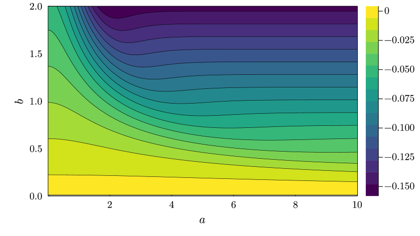
Figure 1: The Ricci curvature $R$ (upper panel) and the potential $V$ (lower panel) for the sine-Gordon KK moduli space with coordinates $(a,b)$. At $a=0$ there is an apparent boundary, reachable after a finite time.

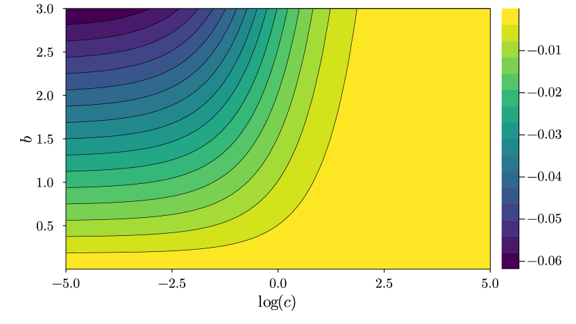
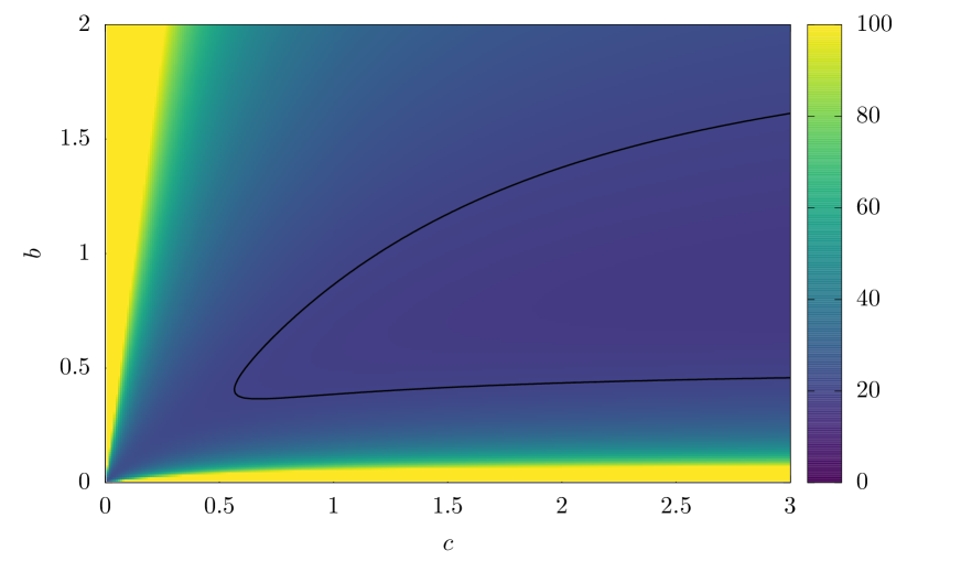
Figure 2: The Ricci curvature $R$ (upper panel) and the potential $V$ (lower panel) for the extended sine-Gordon KK moduli space with coordinates $(c,b)$. The region $c\in(0,1)$ was excluded in Fig. 1. At the boundary $c=0$ the potential diverges.

For the KK configurations (V.6), we obtain a two-dimensional CCM of the general form

$$L[a,b]=\frac{1}{2}g_{aa}\dot{a}^{2}+g_{ab}\dot{a}\dot{b}+\frac{1}{2}g_{bb}\dot{b}^{2}-V(a,b)\,.$$ (V.7)

We find, by integration, that the metric is non-diagonal and has components

$$g_{aa} = 16b\left(1-\frac{2ab}{\sinh(2ab)}\right),$$

$$g_{ab} = -16a\frac{2ab}{\sinh(2ab)}\,,$$

$$g_{bb} = \frac{4\pi^{2}}{3b^{3}}\left[1+\left(1-\frac{8}{\pi^{2}}(ab)^{2}\right)\frac{2ab}{\sinh(2ab)}\right],\hskip 8.5359pt$$ (V.8)

satisfying the identity (III.7), and that the potential is

$$V(a,b) = 8\Bigg{[}b\left(1+\frac{2ab}{\sinh(2ab)}\right)$$ (V.9)

$$\quad+\frac{1}{b\tanh^{2}(ab)}\left(1-\frac{2ab}{\sinh(2ab)}\right)\Bigg{]}\,.$$

The CCM supports a simple solution

$$b=\gamma,\;\;\;a=\frac{1}{\gamma}\mbox{arcosh}\frac{\cosh(\gamma vt)}{v}\,,$$ (V.10)

which, when inserted into (V.6), reproduces the exact kink-kink solution (V.5). In fact, this result can be anticipated by directly comparing the exact solution and the restricted set of configurations (V.6).

Let us now have a closer look at the KK moduli space $\mathcal{M}$. As expected, for $a\to\infty$ it models two independent relativistic solitons, and therefore the CCM has twice the Lagrangian (V.4). On the other hand, $\mathcal{M}$ naively has a boundary at $a=0$, because two of the metric components have zeros:

$$g_{aa}=\frac{32b^{3}}{3}a^{2}+O(a^{4})\,,\quad g_{ab}=-16a+O(a^{3})\,.$$ (V.11)

However, this is only an apparent singularity. Indeed, the Ricci curvature remains finite at $a=0$, see Fig. 1. This null vector problem, resulting from the vanishing of $\partial_{a}\Phi$ as $a\to 0$, can be resolved by a more appropriate choice of coordinates, leading not only to well behaved metric functions but also, importantly, allowing us to extend the moduli space beyond $a=0$.

The resolution is achieved by reparametrizing the configurations (V.6) as

$$\tilde{\Phi}_{KK}(x;c,b)=4\arctan\frac{\sinh bx}{c}\,,$$ (V.12)

where the new collective coordinate $c$ is related to the old ones via $c=\cosh(ba)$. The metric components are now

$$g_{cc} = \frac{16}{b}\frac{1}{c^{2}-1}\left(1-\frac{1}{c\sqrt{c^{2}-1}}\mbox{arcoth}\frac{c}{\sqrt{c^{2}-1}}\right)\,,$$

$$g_{cb} = -\frac{16}{b^{2}}\frac{1}{\sqrt{c^{2}-1}}\mbox{arcoth}\frac{c}{\sqrt{c^{2}-1}}\,,$$

$$g_{bb} = -\frac{4}{b^{3}}\frac{1}{\sqrt{c^{2}(c^{2}-1)}}\left(-\sqrt{c^{2}(c^{2}-1)}\left(\ln^{2}(\tilde{c})+\frac{\pi^{2}}{3}\right)\right.$$ (V.13)

$$+ \left.\frac{1}{6}\ln^{3}(\tilde{c})+\frac{\pi^{2}}{6}\ln(\tilde{c})\right)\,,$$

where

$$\tilde{c}=-1+2c^{2}-2\sqrt{c^{2}(c^{2}-1)}\,,$$ (V.14)

and they are regular on the line $c=1$, which corresponds to $a=0$. Since the potential $V$ also has a finite value on the line, we can extend the moduli space to $c<1$. The curvature and potential extended to the interval $c\in(0,1)$ are shown in Fig. 2. This interval is accessible in a finite time if the initial state has sufficient oscillatory energy. Interestingly, this interval of the moduli space can also be obtained in the previous construction, but requires imaginary values of the coordinate $a$ in the range $(0,i\pi/2b)$.

The boundary at $c=0$ is unattainable since the potential

$$V(c,b) = \frac{8}{bc\left(c^{2}-1\right)^{3/2}}\Biggl{(}c\sqrt{c^{2}-1}\left(b^{2}\left(c^{2}-1\right)+c^{2}\right)$$ (V.15)

$$+ \left(b^{2}\left(c^{2}-1\right)-c^{2}\right)\mbox{arcoth}\left(\frac{c}{\sqrt{c^{2}-1}}\right)\Biggr{)}$$

diverges as $c\to 0$. A second line of $\mathcal{M}$ where the metric behaves badly is $b=0$. This is also a true boundary towards which the potential diverges, so no finite-energy KK trajectories reach it.

To conclude, the extended relativistic moduli space provides a well defined dynamical system for KK dynamics in the sG model, as well as reproducing the exact KK scattering solution.

V.2 Kink-antikink solution

We turn now to the kink-antikink (KAK) solutions of the sG model, both the scattering solution

$$\Phi_{KAK}(x,t)=4\arctan\frac{\sinh(\gamma vt)}{v\cosh(\gamma x)}$$ (V.16)

and the breather

$$\Phi_{B}(x,t)=4\arctan\left(\frac{\sqrt{1-\omega^{2}}}{\omega}\frac{\sin(\omega t)}{\cosh(\sqrt{1-\omega^{2}}\,x)}\right)\,,$$ (V.17)

where $0<\omega<1$.

These solutions can be obtained by using the KAK superposition

$$\Phi_{KAK}(x;a,b) = 4\arctan e^{b(x+a)}-4\arctan e^{b(x-a)}$$ (V.18)

$$= 4\arctan\frac{\sinh ba}{\cosh bx}\,.$$

Here, the configurations are not symmetric under $a\mapsto-a$, so $a$ can have any real value. However, there is a symmetry under the combined transformation $a\mapsto-a$ and $b\mapsto-b$, so it makes sense to require $b>0$. The configuration with $b=0$ is the vacuum configuration for any $a$, but this configuration also occurs for $a=0$ with $b>0$.

The restricted set of configurations (V.18) defines the KAK moduli space $\mathcal{M}$ with metric components

$$g_{aa} = 16b\left(1+\frac{2ab}{\sinh(2ab)}\right),$$

$$g_{ab} = 16a\frac{2ab}{\sinh(2ab)}\,,$$

$$g_{bb} = \frac{4\pi^{2}}{3b^{3}}\left[1-\left(1-\frac{8}{\pi^{2}}(ab)^{2}\right)\frac{2ab}{\sinh(2ab)}\right],\hskip 8.5359pt$$ (V.19)

and potential

$$V(a,b)= 8 \left[b\left(1-\frac{2ab}{\sinh(2ab)}\right)\right.$$ (V.20)

$$+ \left.\frac{\tanh^{2}(ab)}{b}\left(1+\frac{2ab}{\sinh(2ab)}\right)\right]\,.$$

The identity (III.7) is again satisfied. Contrary to the KK case, the potential is finite, see Fig. 3. However, for $a\neq 0$, the configurations with $b\to 0$ are rather far from the physical regime $b\approx 1$, so are unimportant for KAK scattering.

The relativistic CCM has the solution

$$b=\gamma\,,\quad a(t)=\frac{1}{\gamma}\mbox{arsinh}\frac{\sinh(\gamma vt)}{v}\,,$$ (V.21)

fully reproducing the analytical KAK scattering solution for all velocities. As before, it can be obtained by comparing the exact solution with the restricted configurations (V.18). For the breather solution,

$$b = \sqrt{1-\omega^{2}}\,,$$

$$a(t) = \frac{1}{\sqrt{1-\omega^{2}}}\mbox{arsinh}\left(\frac{\sqrt{1-\omega^{2}}}{\omega}\sin(\omega t)\right).$$ (V.22)

V.3 KK and KAK moduli spaces compared

The KAK moduli space has metric components $g_{ab}$ and $g_{bb}$ whose behaviour for small $a$ is

$$g_{ab} = 16a+O(a^{3})\,,$$

$$g_{bb} = \frac{8}{9b}(12+\pi^{2})a^{2}+O(a^{4})\,.$$ (V.23)

These components vanish at $a=0$, producing a metric singularity, whereas it was $g_{aa}$ and $g_{ab}$ that vanished at $a=0$ in the KK case. The Ricci curvature is still finite for all $a$ and $b$, see Fig. 3.

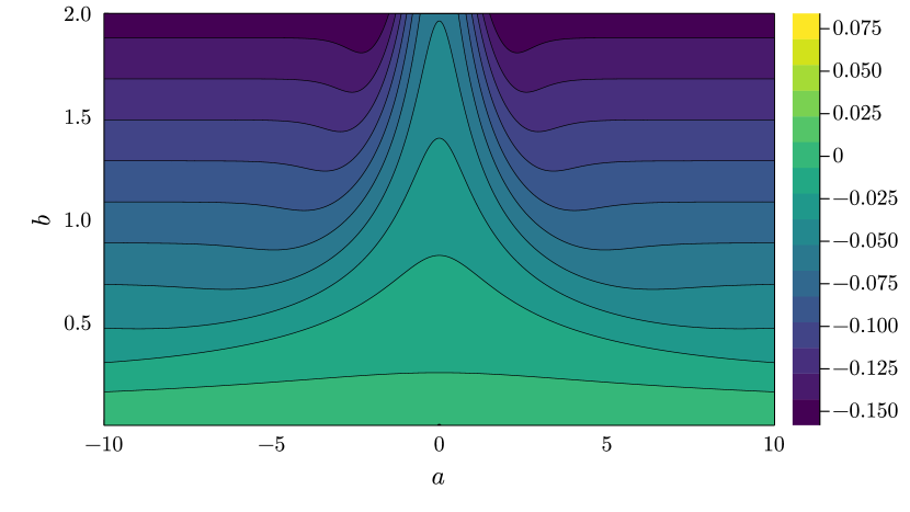
Figure 3: The Ricci curvature $R$ (upper panel) and the potential $V$ (lower panel) for the KAK moduli space in the sine-Gordon model. The boundary at $b=0$, containing a possible singularity, is not included.

This suggests the KK and KAK sectors have different types of null vector. To understand this better, we expand the restricted configurations $\Phi_{KK}$ and $\Phi_{KAK}$ for small $a$, finding

$$\Phi_{KK}(x;a,b) = 4\arctan(\sinh(bx))$$

$$\quad-\frac{2\sinh(bx)}{1+\sinh^{2}(bx)}b^{2}a^{2}+O(a^{4})$$

and

$$\Phi_{KAK}(x;a,b)=\frac{4}{\cosh(bx)}ba+O(a^{3})\,.$$ (V.25)

For $\Phi_{KK}$ the derivative w.r.t. $a$ vanishes as $a\to 0$, while for $\Phi_{KAK}$ it is the derivative w.r.t. $b$. In the former case it was sufficient to introduce the coordinate $c=\cosh(ba)\approx 1+\frac{1}{2}b^{2}a^{2}$, but this does not help in the latter case, where the singularity is essential, as we argued in Section III.

We recall here that there exists a relativistic model of two interacting point particles on the line, whose dynamics precisely reproduces the kink-kink (or kink-antikink) solution of the sine-Gordon model. This is the famous Ruijsenaars–Schneider model with a particular pair potential RS . Undoubtedly, it would be very interesting to understand possible relations between this model and the relativistic CCM.

V.4 Perturbative framework applied to sG model

Here we set $b=1+\epsilon$ and expand in $\epsilon$. For the single sG kink we find

$$\Phi_{K}(x;a,b)=4\arctan e^{b(x-a)}=4\arctan e^{(x-a)}$$ (V.26)

$$\qquad+\epsilon\frac{2(x-a)}{\cosh(x-a)}-\epsilon^{2}\frac{(x-a)^{2}\tanh(x-a)}{\cosh(x-a)}+o(\epsilon^{2})\,.$$

The set of configurations up to first order is therefore

$$\Phi_{K}(x;a,C)=4\arctan e^{(x-a)}+C\frac{2(x-a)}{\cosh(x-a)}$$ (V.27)

where $C\equiv C_{1}$. Their two-dimensional moduli space has a diagonal metric with components

$$g_{aa} = 8+8C+\frac{2}{9}(12+\pi^{2})C^{2}\,,$$

$$g_{CC} = \frac{2\pi^{2}}{3}\,.$$ (V.28)

The quadratic character of $g_{aa}$ makes this a wormhole-type metric.

Figure 4: KAK collision in the pRCCM for the sine-Gordon model with moduli $(a,C)$. Left: $a(t)$; Center: $C(t)$; Right: Difference between $a(t)$ obtained in the pRCCM and the exact expression $a_{exact}(t)$. From top to bottom $v=0.2,0.4,0.6$, and $0.8$.

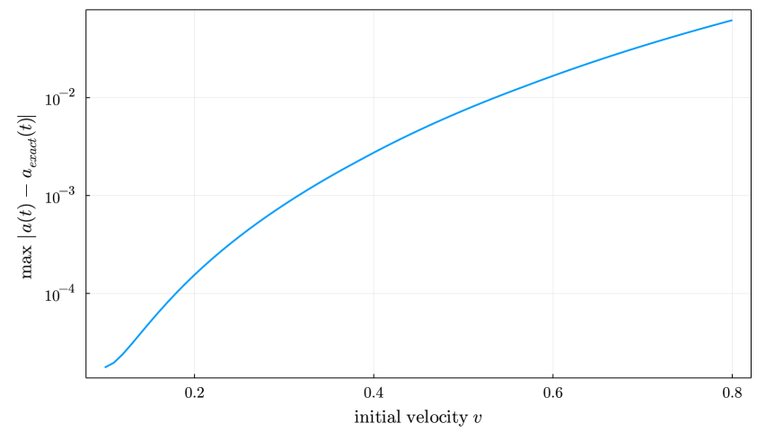
Figure 5: Maximum of the difference between $a(t)$ obtained in the pRCCM for the sine-Gordon model and the exact expression $a_{exact}(t)$, as a function of $v$.

The potential, up to fourth order in $C$, is

$$V(C) = 8+4C^{2}+\frac{2}{9}\left(\pi^{2}-6\right)C^{3}$$ (V.29)

$$+ \frac{1}{450}\left(240-100\pi^{2}+7\pi^{4}\right)C^{4}\,.$$

Importantly, the equations of motion of the resulting pRCCM have a stationary solution satisfying

$$\ddot{a} = 0\,,$$ (V.30)

$$\frac{1}{2}\partial_{C}g_{aa}\,{\dot{a}}^{2} = \partial_{C}V\,.$$ (V.31)

The first equation has the constant-velocity solution $\dot{a}=v$, while the second becomes the nonlinear algebraic equation

$$0 = 4v^{2}+\left(\frac{2}{9}\left(12+\pi^{2}\right)v^{2}-8\right)C$$

$$- \frac{2}{3}\left(\pi^{2}-6\right)C^{2}-\frac{2}{225}\left(240-100\pi^{2}+7\pi^{4}\right)C^{3}\,,$$

with a real solution whose truncated expansion is

$${\tilde{C}}\approx 0.5v^{2}+0.223127v^{4}+0.072637v^{6}+0.016753v^{8}\,.$$ (V.33)

This expansion reproduces the true value of $C$ with good precision.

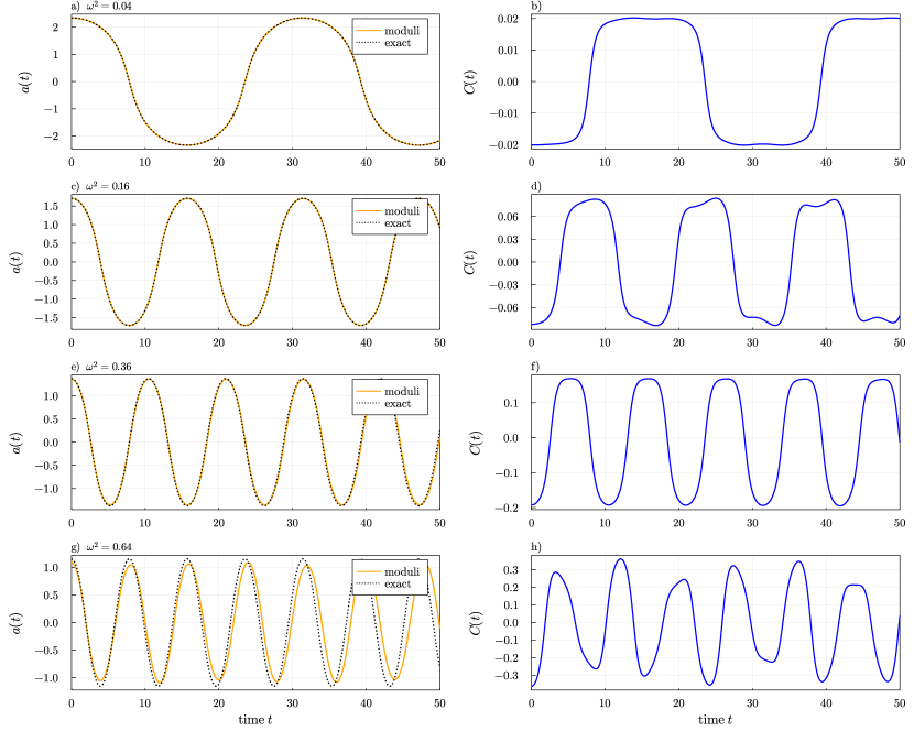
Figure 6: Oscillatory solutions $a(t)$ (left) and $C(t)$ (right) of the pRCCM for the sine-Gordon model. Here (from top to bottom) $\omega^{2}=0.04,0.16,0.36$, and $0.64$. The dotted line represents $a(t)$ computed from the exact breather solution.

Obviously by enlarging the model, taking into account more terms in the expansion, we approach the exact Lorentz-boosted kink with arbitrary accuracy. The price is the growing dimension of the moduli space and the complexity of the resulting equations.

Although the perturbative expansion seems to be an unnecessary complication for a single kink, its usefulness becomes clear when we apply it to the KAK solutions in sG. We consider only the terms up to first order, using the moduli $(a,C)$. The restricted set of configurations, where the null vector is already removed, is

$$\Phi_{KAK}(x;a,C)=4\arctan e^{(x+a)}-4\arctan e^{(x-a)}$$

$$\quad+\frac{2C}{\tanh(a)}\left(\frac{x+a}{\cosh(x+a)}-\frac{x-a}{\cosh(x-a)}\right)\,.$$ (V.34)

The resulting metric is non-singular for any finite $(a,C)$, but as the formulae for the metric components are very long, we do not present them. Furthermore, in our numerical investigations of KAK dynamics we obtain the metric and potential numerically, not referring to their analytical formulae (see Appendix A). In this way, we arrive at a well defined two-dimensional pRCCM for modelling KAK collisions in the underlying field theory. This procedure could be repeated up to any order $n$.

We also need appropriate initial conditions for the approaching kink and antikink. These are provided by the moving single-kink solution of the pRCCM with $C$ given by (V.33), which leads to the following initial conditions at $t=0$,

$$a(0) = a_{0},\;\;\dot{a}(0)=v,$$

$$C(0) = 0.5v^{2}+0.223127v^{4}+0.072637v^{6}+0.016753v^{8},$$

$$\dot{C}(0) = 0\,,$$ (V.35)

where $a_{0}$ is half the initial distance between the solitons.

In Fig. 4, left and center column, we present the time evolution of $a(t)$ and $C(t)$ obtained in the pRCCM, based on the configurations (V.34) and the initial conditions (V.35). The initial velocity has the range of values $v=0.2,0.4,0.6$, and $0.8$. For comparison, we also plot the position of the kink (and antikink) obtained from the sG KAK solution $a_{exact}(t)$ given in (V.21).

To better see the agreement between the pRCCM computation and the exact solution, we plot the difference $a(t)-a_{exact}(t)$ in Fig. 4, right column. The difference is small even for quite relativistic velocities. E.g., for $v=0.4$ the maximum difference is about $0.003$, while at large times it oscillates between $\pm 0.001$.

In Fig. 5 we plot the maximum of this difference as a function of the initial velocity $v$. For small velocities, where our first-order relativistic approximation should work well, the agreement is extremely good. E.g., for $v\lesssim 0.2$ the difference is less than $10^{-4}$. This should be compared with the one-dimensional moduli space computation where for $v=0.2$ the corresponding difference is of order $10^{-2}$ zero-vec . Hence, the inclusion of the first Derrick mode leads to results which are two orders of magnitude more precise.

It is also important to notice that the inclusion of the Derrick mode does not spoil the integrability of the model. The result of the KAK scattering is always a KAK pair. We do not observe any bounce windows or bion formation. This is obviously a crucial test for the validity of our perturbative relativistic framework.

The same pRCCM can be used to study the breather solution, provided the initial conditions have energy less than twice the static energy of a kink. In Fig. 6 we present examples of oscillatory solutions $(a(t),C(t))$. The coordinate $a(t)$ is also compared with the exact expression (V.22) derived from the breather solution. We find good agreement for $\omega\ll 1$. For larger frequencies we notice some discrepancy. There is also a departure from exact periodicity. In any case, it is an important result in our framework that the addition of the new collective coordinate does not lead to the disappearance of the bound orbits. It should be underlined that in the one-dimensional CCM zero-vec the existence of periodic solutions is guaranteed if the energy condition for a breather is satisfied. In higher-dimensional moduli spaces, on the other hand, it is a nontrivial phenomenon, which relies on the details of the moduli space metric and potential.

VI $\phi^{4}$ theory

We consider next the prototypical, non-integrable scalar field theory supporting topological solitons, the $\phi^{4}$ theory in (1+1)-dimensional space-time. The Lagrangian is

$$L_{\phi^{4}}[\phi]=\int_{-\infty}^{\infty}dx\left(\frac{1}{2}(\partial_{t}\phi)^{2}-\frac{1}{2}(\partial_{x}\phi)^{2}-\frac{1}{2}(1-\phi^{2})^{2}\right)\,,$$ (VI.1)

and the field equation has the static BPS kink solutions

$$\Phi_{K}(x;a)=\tanh(x-a)$$ (VI.2)

interpolating between the vacua $-1$ and $+1$. The modulus $a\in\mathbb{R}$ is the position of the kink, and the resulting canonical moduli space has the constant metric $g_{aa}=M=4/3$, so the CCM Lagrangian is

$$L[a]=\frac{2}{3}\dot{a}^{2}-\frac{4}{3}\,.$$ (VI.3)

In this description, the kink moves at an arbitrary velocity $v$ as a non-relativistic particle with mass $M$ and the Lorentz invariance of the original field theory is lost. The antikink $\Phi(x;a)=-\tanh(x-a)$ interpolates between $+1$ and $-1$, but otherwise has similar properties to the kink.

The $\phi^{4}$ kink has one positive-frequency normal mode, the normalized shape mode

$$\eta_{sh}(x)=\frac{3}{2}\frac{\sinh(x)}{\cosh^{2}(x)}\,,$$ (VI.4)

whose frequency $\omega^{2}_{sh}=3$ is below the continuum threshold $\omega^{2}=4$. This mode plays a distinguished role in multi-kink dynamics in $\phi^{4}$ theory.

VI.1 Relativistic Moduli Space

Including the Derrick scaling deformation, with modulus $b>0$, the single-kink configurations are

$$\Phi_{K}(x;a,b)=\tanh b(x-a)\,.$$ (VI.5)

The resulting two-dimensional moduli space has the diagonal metric

$$g_{aa}=\frac{4}{3}b\,,\quad g_{bb}=\frac{\pi^{2}-6}{9}\frac{1}{b^{3}}\,,$$ (VI.6)

and potential

$$V(b)=\frac{2}{3}\left(b+\frac{1}{b}\right)\,,$$ (VI.7)

so the relativistic CCM combining these has Lagrangian

$$L[a,b]=\frac{2}{3}b\dot{a}^{2}+\frac{\pi^{2}-6}{18b^{3}}\dot{b}^{2}-\frac{2}{3}\left(b+\frac{1}{b}\right)\,.$$ (VI.8)

As before, the equations of motion have solutions describing relativistic, Lorentz-contracted kinks moving at constant velocity.

The normalized Derrick mode is now

$$\eta_{D}(x)=\frac{3}{\sqrt{\pi^{2}-6}}\frac{x}{\cosh^{2}(x)}\,,$$ (VI.9)

which is known to be almost identical to the shape mode MORW . Indeed, the Derrick mode frequency $\omega_{D}^{2}=12/(\pi^{2}-6)\approx 3.101$ is very close to the shape mode frequency, and the inner product of the normalized Derrick and shape modes $(\eta_{D},\eta_{sh})\approx 0.98$ is very close to unity.

Exactly as in the sine-Gordon case, the construction of a relativistic CCM describing KAK collisions encounters difficulties. The superposition of kink and antikink,

$$\Phi_{KAK}(x;a,b)=\tanh b(x+a)-\tanh b(x-a)-1\,,$$ (VI.10)

leads to a CCM with metric components

$$g_{aa} = b\left[\frac{8}{\sinh^{2}(2ab)}\left(-1+\frac{2ab}{\tanh(2ab)}\right)+\frac{8}{3}\right],$$ (VI.11)

$$g_{ab} = \frac{8a}{\sinh^{2}(2ab)}\left(-1+\frac{2ab}{\tanh(2ab)}\right),$$

$$g_{bb} = \frac{2}{9b^{3}}\Biggl{[}\pi^{2}-6$$

$$+\frac{3}{\sinh^{2}(2ab)}\left(\pi^{2}-\frac{2ab}{\tanh(2ab)}(\pi^{2}-8a^{2}b^{2})\right)\Biggr{]},$$

and potential

$$V(a,b) = \frac{4b}{3}\Biggl{[}\frac{3}{\sinh^{2}(2ab)}\left(1-\frac{2ab}{\tanh(2ab)}\right)+1\Biggr{]}$$

$$+ \frac{4}{3b}\Biggl{[}-17-24ab-\frac{3(5+12ab)}{\sinh^{2}(2ab)}$$

$$+ \frac{6}{\tanh(2ab)}\left(3+4ab+\frac{5ab}{\sinh^{2}(2ab)}\right)\Biggr{]}\,.$$

The metric components satisfy (III.7), and once again the Ricci curvature is finite for any $a\in\mathbb{R}$ and $b>0$, but the metric still degenerates at $a=0$. There is a null vector problem at $a=0$, because the field configurations (VI.10) become the vacuum, which has zero derivative w.r.t. $b$. However, as argued earlier, there is no simple resolution of this singularity. The configuration space for $a>0$ is a smooth two-dimensional manifold, and similarly for $a<0$. These two surfaces are glued together at the single point $a=0$, and the result is singular.

If we introduce the coordinate $c=ab$ in (VI.10), then

$$\Phi_{KAK}(x;b,c)=\tanh(bx+c)-\tanh(bx-c)-1\,.$$ (VI.13)

The corresponding metric components on the moduli space are

$${\tilde{g}}_{bb} = \frac{2}{9b^{3}}\Biggl{[}12c^{2}+\pi^{2}-6$$

$$+ \frac{3}{\sinh^{2}(2c)}\left(12c^{2}+\pi^{2}-\frac{2c}{\tanh(2c)}\left(4c^{2}+\pi^{2}\right)\right)\Biggr{]}\,,$$

$${\tilde{g}}_{bc} = -\frac{8}{3}\frac{c}{b^{2}}\,,$$

$${\tilde{g}}_{cc} = \frac{1}{b}\left[\frac{8}{\sinh^{2}(2c)}\left(-1+\frac{2c}{\tanh(2c)}\right)+\frac{8}{3}\right]\,,$$ (VI.14)

which satisfy the identity (III.9), and the potential $V$ simplifies when expressed in terms of $b$ and $c$.

VI.2 Perturbative approach to KAK collisions

To avoid the singularity at $a=0$, we use the perturbative approach. As before, we begin with the Derrick deformed single kink $\Phi_{K}=\tanh((1+\epsilon)(x-a))$ with modulus $b=1+\epsilon$, and perform an expansion in $\epsilon$. If we keep only the first Derrick mode $\eta_{D}$, then

$$\Phi_{K}(x;a,C)=\tanh(x-a)+C\frac{x-a}{\cosh^{2}(x-a)}\,,$$ (VI.15)

where we have identified $C=\epsilon$. These configurations have a moduli space with the diagonal metric

$$g_{aa} = \frac{4}{3}+\frac{4}{3}C+\frac{4\pi^{2}}{45}C^{2}\,,$$

$$g_{CC} = \frac{\pi^{2}-6}{9}\,,$$ (VI.16)

and the potential

$$V(C) = \frac{4}{3}+\frac{2}{3}C^{2}+\frac{1}{45}(4\pi^{2}-30)C^{3}$$ (VI.17)

$$+ \frac{1}{450}(120-70\pi^{2}+6\pi^{4})C^{4}\,.$$

As in the case of the sG kink, the pRCCM has a stationary solution obeying the equations of motion (V.30) and (V.31). Specifically, the equation for $C$ reads

$$0 = \frac{2v^{2}}{3}+\frac{4}{45}(\pi^{2}v^{2}-15)C-\frac{1}{15}(4\pi^{2}-30)C^{2}$$ (VI.18)

$$- \frac{2}{225}(120-70\pi^{2}+6\pi^{4})C^{3}\,,$$

when we set $\dot{a}=v$. This can be solved exactly, but as the solution has a long, unilluminating form, we use its truncated expansion in $v^{2}$,

$${\tilde{C}}\approx 0.5v^{2}+0.210507v^{4}+0.027428v^{6}-0.0302351v^{8}\,,$$ (VI.19)

in our numerical simulations.

Keeping the first two Derrick modes, the single-kink configurations are

$$\Phi_{K}(x;a,{\bf C}) = \tanh(x-a)+C_{1}\frac{x-a}{\cosh^{2}(x-a)}$$ (VI.20)

$$- C_{2}(x-a)^{2}\frac{\tanh(x-a)}{\cosh^{2}(x-a)}\,,$$

which leads to a pRCCM with three moduli,

$$L[a,{\bf C}]=\frac{1}{2}g_{aa}\dot{a}^{2}+\frac{1}{2}g_{ij}\dot{C}_{i}\dot{C}_{j}-V({\bf C})\,.$$ (VI.21)

Here we explicitly use the fact that $g_{ai}=0$, $i=1,2$. Although the metric functions and the potential can be found analytically, the formulae are again long, so we do not display them. In any case, in our calculations they are computed numerically. There is a stationary solution approximating the boosted kink moving at constant velocity $\dot{a}=v$, having non-zero Derrick mode amplitudes $\tilde{C}_{k}$ determined using the algebraic equations

$$\frac{1}{2}\partial_{C_{k}}g_{aa}v^{2}=\partial_{C_{k}}V\,.$$ (VI.22)

We turn now to kink-antikink (KAK) collisions, and compare the results from the pRCCM keeping either one or two Derrick moduli to results from full field theory simulations, and also to the results found in ref.MORW using the CCM based on the shape mode.

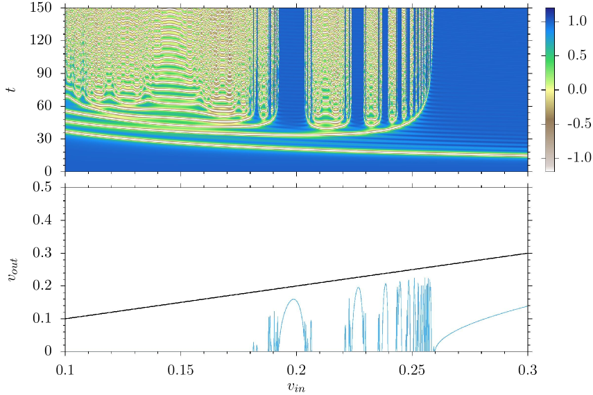
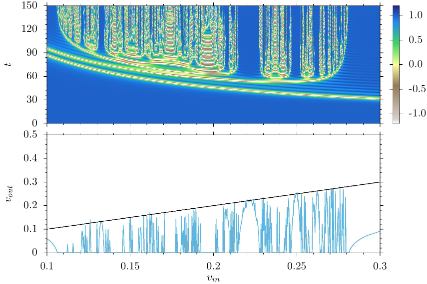
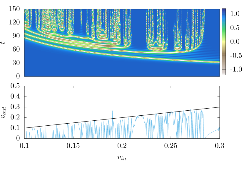
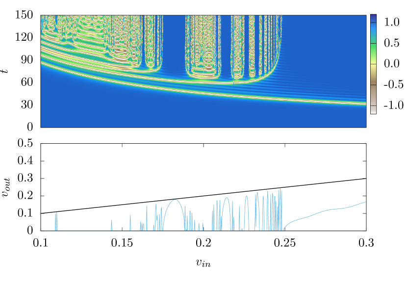
Figure 7: KAK collision in $\phi^{4}$ theory: time dependence of the field at the origin, $\phi(x=0,t)$, and final velocity of backscattered antikink $v_{out}$ for various initial velocities $v_{in}$. Upper left: the full field theory dynamics; upper right: the CCM based on the shape mode MORW ; lower left: the pRCCM with moduli $(a,C)$; lower right: the pRCCM with moduli $(a,C_{1},C_{2})$.

The configurations in the pRCCM are kink-antikink superpositions expanded to finite order in the Derrick modes,

$$\Phi_{KAK}(x;a,{\bf C})=\Phi_{K}(x;-a,{\bf C})-\Phi_{K}(x;a,{\bf C})-1\,.$$ (VI.23)

Inserting these into the $\phi^{4}$ theory Lagrangian gives

$$L_{KAK}(a,{\bf C})=\int_{-\infty}^{\infty}\mathcal{L}_{\phi^{4}}[\Phi_{KAK}(x;a,{\bf C})]\,dx\,,$$ (VI.24)

and after integrating over $x$ we obtain the Lagrangian of the pRCCM, which is a well defined dynamical system provided the null-vector problems are cured by redefining the moduli via

$$C_{k}\mapsto\frac{C_{k}}{\tanh(a)}\,.$$ (VI.25)

The resulting second-order equations of motion for the moduli require initial conditions

$$a(0)=a_{0},\;\;\dot{a}(0)=v\,,$$

$$C_{k}(0)=\tilde{C}_{k},\;\;\dot{C}(0)=0\,,$$ (VI.26)

corresponding to a well-separated KAK pair boosted towards each other.

More explicitly, the configurations modelling KAK collisions with just one Derrick mode are

$$\Phi_{KAK}(x;a,C)=\tanh(x+a)-\tanh(x-a)-1$$ (VI.27)

$$+ \frac{C}{\tanh(a)}\left(\frac{x+a}{\cosh^{2}(x+a)}-\frac{x-a}{\cosh^{2}(x-a)}\right)\,.$$

The resulting pRCCM has equations of motion that must be supplemented by the single-kink initial conditions

$$a(0) = a_{0}\,,\quad\dot{a}(0)=v\,,$$

$$C(0) = 0.5v^{2}+0.210507v^{4}+0.027428v^{6}-0.0302351v^{8}\,,$$

$$\dot{C}(0) = 0\,.$$ (VI.28)

In the full $\phi^{4}$ field theory simulations of KAK collisions, the kink and antikink are boosted towards each other at speeds $v_{in}$, through the initial conditions

$$\phi_{in}(x,0)=\tanh(\gamma(x+a_{0}))-\tanh(\gamma(x-a_{0}))-1\,,$$

$$\partial_{t}\phi_{in}(x,0)=\frac{\gamma v_{in}}{\cosh^{2}(\gamma(x+a_{0}))}-\frac{\gamma v_{in}}{\cosh^{2}(\gamma(x+a_{0}))}\,.$$

In the field theory the kink and antikink either perform a few bounces before escaping to infinity, or they annihilate to the vacuum via the formation of an oscillating state, called a bion, which slowly radiates, decaying to the vacuum. Interestingly, these two possibilities exhibit an amazingly complicated pattern depending on the incoming soliton velocities, with multi-bounce windows and bion chimneys occurring in a fractal manner, see Fig. 7, upper left panel. The fractal structure starts at $v_{min}\approx 0.18$ and ends at $v_{crit}=0.2598$. Below $v_{min}$ only bion chimneys exist, while above $v_{crit}$ only one-bounce scattering is observed.

For a comparison with the non-relativistic CCM based on the shape mode MORW , see Fig. 7, upper right panel. The fractal structure is qualitatively reproduced but there are important details which do not fully agree: (i) there is an overall shift toward larger values of $v_{in}$, e.g., $v_{crit}\approx 0.28$; (ii) there is an unwanted, wide two-bounce window that dominates the low-velocity dynamics for $v_{in}\lesssim 0.11$; (iii) there are many three-bounce and higher-bounce windows in the field theory’s bion regime, i.e., for $0.11\lesssim v_{in}\lesssim 0.2$. Of course, the appearance of bounce windows with a large number of bounces is unsurprising as the CCM has no radiation modes that could transfer energy from the bion. In the CCM, bions can decay only to a free KAK pair. However, the existence of additional two-, three- or four-bounce windows is a rather unwanted feature. Despite this, the results provide convincing evidence that resonant energy transfer between kink motion and an oscillatory mode is the mechanism responsible for the observed fractal structure in the final state formation.

The dynamics found in the pRCCM with only one Derrick modulus $C$ looks similar, see Fig. 7, lower left panel. The overall shift to higher velocities persists, e.g., $v_{crit}=0.2853$. The velocity shift compared with the field theory is $\Delta v_{crit}=0.0255$, a $10\%$ error. However, there is an important improvement in the low-velocity regime, as the number of unwanted low-velocity bounce windows is drastically reduced. Specifically, there is no low-velocity two-bounce window and there is only one unwanted three-bounce window.

A spectacular improvement is observed if we use the pRCCM keeping two Derrick moduli $C_{1}$ and $C_{2}$, see Fig. 7, lower right panel. Basically, almost all bions in the bion chimneys behave as in the field theory, i.e., they do not decay into free solitons after just a small number of bounces. Hence, there are very few bounce windows in the low-velocity regime, and each exhibits a large number of bounces. A similar improvement is observed in the higher-velocity regime. Furthermore, the critical velocity is substantially reduced, to $v_{crit}=0.2490$, for which $\Delta v_{crit}=0.0108$, which is only a $4\%$ error. Additionally, the small wiggles in the final velocities of the solitons, occurring in both the two-dimensional CCMs, are now absent.

Interestingly, the frequency of the first Derrick mode tends to the frequency of the shape mode as the dimension of the pRCCM increases. Specifically, it decreases from $\omega^{2}_{1}=3.1011$ to $\omega^{2}_{1}=3.0221$ when the modulus $C_{2}$ is included. In the latter case, the second Derrick mode has frequency $\omega^{2}_{2}=6.9283$, which is above the continuum threshold. Therefore, oscillations of this mode may partially simulate some aspects of radiation.

VII Conclusions

In the present work we have explored the relativistic collective coordinate model for (multi-)kink dynamics, which arises when the Derrick scaling deformation with modulus (scale parameter) $b>0$ is included. For a moving single kink the model reproduces the Lorentz contraction of the kink Rice , and its reduced Lagrangian is that of a relativistic point particle.

The model can be extended to kink-kink (KK) and kink-antikink (KAK) collisions. For the KK sector of the sine-Gordon model, we have constructed a globally well defined moduli space whose metric and potential lead to a Lagrangian reproducing the exact KK solution.

In the case of general KAK dynamics, the construction encounters some difficulties. The moduli space has a metric singularity at $a=0$, i.e., when the kink and antikink coincide and pass through the vacuum solution. We have shown that this is an essential geometric singularity that cannot be removed by a redefinition of the collective coordinates.

To circumvent this issue, we have introduced a perturbative version of the relativistic collective coordinate model (pRCCM), where the Derrick modulus is expanded around its undeformed value $b=1$. This corresponds to an expansion in the squared kink velocity, and therefore incorporates relativistic corrections in a perturbative manner. Here, a key idea is to treat all the terms in the field expansion as independent higher-order Derrick modes whose amplitudes are independent collective coordinates. The field configurations are less constrained than before, even if just the first-order (original) Derrick mode is retained. Each of these new collective coordinates has a null vector problem at $a=0$, but these can all be resolved by a coordinate redefinition that absorbs a factor $\tanh(a)$. Note that such a coordinate redefinition has no physical effect for $a>0$, but it smoothly extends the moduli space through $a=0$ and allows for a smooth dynamics.

In contrast to previous treatments of the singularity of the relativistic CCM, this is a straightforward approach that can easily be implemented. Furthermore, it provides an arbitrary number of collective coordinates, which can be used to improve the description of multi-kink collisions in any (1+1)-dimensional scalar field theory. It has been tested in the sG model and in $\phi^{4}$ theory, and the results are very encouraging.

In the case of KAK collisions in the sG model, we found that the pRCCM does not spoil the integrability property. The inclusion of the first Derrick mode gives a model where there is always a separating kink and antikink in the final state. There is no annihilation or particle production, as expected. In fact, the two-dimensional pRCCM gives a more accurate approximation, by two orders of magnitude, than the simpler one-dimensional CCM constructed from a superposition of an undeformed kink and antikink.

The pRCCM framework, applied to KAK collisions in $\phi^{4}$ theory, reproduces the fractal structure of the velocity-dependence of the final state formation rather well. When the first-order Derrick mode is included, there is a small improvement in comparison with the CCM incorporating the kink’s shape mode MORW . The improvement is particularly striking when both the first-order and second-order Derrick modes are included. The results from the pRCCM appear to be converging to those of the field theory as the number of retained Derrick modes increases.

This shows the universality of the Derrick deformation framework. Namely, it works for qualitatively distinct kinks, one having a shape mode, and the other not. It would be interesting to extend this relativistic framework to field theories with kinks that are not spatially antisymmetric, e.g., to the kinks of the $\phi^{6}$ model.

Finally, one would like to extend the framework to higher dimensions. For example, in the context of (3+1)-dimensional Skyrmions, it may improve the vibrational quantization procedure chris . This is, of course, related to the question of possible quantum corrections to kink dynamics, recently reconsidered by Evslin Jarah . Quantum corrections can contribute to shape mode dynamics, and therefore presumably to the dynamics of Derrick modes at any order.

Appendix A Numerical method for solving the CCM

The collective coordinate model for field configurations $\Phi(x;{\bf X})$ with Lagrangian (II.3) has the Euler–Lagrange equations

$$\ddot{X}^{i}\int_{-\infty}^{\infty}\frac{\partial\Phi}{\partial X^{i}}\frac{\partial\Phi}{\partial X^{k}}\,dx + \dot{X}^{i}\dot{X}^{j}\int_{-\infty}^{\infty}\frac{\partial^{2}\Phi}{\partial X^{i}\partial X^{j}}\frac{\partial\Phi}{\partial X^{k}}\,dx$$ (A.1)

$$= \quad-\int_{-\infty}^{\infty}\frac{\partial W}{\partial X^{k}}\,dx$$

where

$$W(\Phi)=\frac{1}{2}\left(\frac{\partial\Phi}{\partial x}\right)^{2}+U(\Phi)\,.$$ (A.2)

This can be rewritten as a matrix differential equation for the moduli $X^{i}$,

$$\left(\int_{-\infty}^{\infty}e_{i}e_{k}\,dx\right)\ddot{X}^{i} + \left(\int_{-\infty}^{\infty}H_{ij}e_{k}\,dx\right)\dot{X}^{i}\dot{X}^{j}$$ (A.3)

$$\quad=-\int_{-\infty}^{\infty}\frac{\partial W}{\partial X^{k}}\,dx$$

where

$$e_{i}=\frac{\partial\Phi}{\partial X^{i}}\,,\qquad H_{ij}=\frac{\partial^{2}\Phi}{\partial X^{i}\partial X^{j}}\,.$$ (A.4)

In solving this set of equations, it turns out that calculating the integrals numerically, even for the metric integrand $e_{i}e_{k}$, is more stable than implementing analytical expressions. The cost is similar to the cost of calculating the integral on the right hand side, as we need to numerically calculate the vectors $e_{i}$ anyway. Direct analytical calculations are prone to many numerical errors, arising, for example, from the catastrophic cancellation problem. Therefore, we calculated each required integral at every time step.

References

- (1) R. Rajaraman, Solitons and Instantons, Elsevier Science, Amsterdam, 1982.
- (2) N. Manton and P. Sutcliffe, Topological Solitons, Cambridge University Press, Cambridge U.K., 2004.
- (3) Y. M. Shnir, Topological and Non-Topological Solitons in Scalar Field Theories, Cambridge University Press, Cambridge U.K., 2018.
- (4) T. Sugiyama, Kink-antikink collisions in the two-dimensional model, Prog. Theor. Phys. 61 (1979) 1550.
- (5) D. K. Campbell, J. F. Schonfeld, and C. A. Wingate, Resonance structure in kink-antikink interactions in theory, Physica D9 (1983) 1.
- (6) D. K. Campbell, M. Peyrard, and P. Sodano, Kink-antikink interactions in the double sine-Gordon equation, Physica D19 (1986) 165.
- (7) B. A. Malomed, Dynamics and kinetics of solitons in the driven damped double Sine-Gordon equation, Phys. Lett. A136 (1989) 395.
- (8) V. A. Gani and A. E. Kudryavtsev, Kink - anti-kink interactions in the double sine-Gordon equation and the problem of resonance frequencies, Phys. Rev. E60 (1999) 3305.
- (9) R. H. Goodman and R. Haberman, Interaction of sine-Gordon kinks with defects: The two-bounce resonance, Physica D195 (2004) 303.
- (10) R. H. Goodman and R. Haberman, Kink-antikink collisions in the equation: The n-bounce resonance and the separatrix map, SIAM J. Appl. Dyn. Syst. 4 (2005) 1195.
- (11) I. Takyi and H. Weigel, Collective coordinates in one-dimensional soliton model revisited, Phys. Rev. D94 (2016) 085008.
- (12) A. Alonso-Izquierdo, Reflection, transmutation, annihilation, and resonance in two-component kink collisions, Phys. Rev. D97 (2018) 045016.
- (13) P. G. Kevrekidis and R. H. Goodman, Four decades of kink interactions in nonlinear Klein-Gordon models: A crucial typo, recent developments and the challenges ahead, https://dsweb.siam.org/The-Magazine/All-Issues/acat/1/archive/ 102019; arXiv:1909.03128.
- (14) I. C. Christov, R. J. Decker, A. Demirkaya, V. A. Gani, P. G. Kevrekidis, and R. V. Radomskiy, Long-range interactions of kinks, Phys. Rev. D99 (2019) 016010.
- (15) F. C. Simas, F. C. Lima, K. Z. Nobrega, and A. R. Gomes, Solitary oscillations and multiple antikink-kink pairs in the double sine-Gordon model, JHEP 12 (2020) 143.
- (16) A. Alonso-Izquierdo, J. Queiroga-Nunes, and L. M. Nieto, Scattering between wobbling kinks, Phys. Rev. D103 (2021) 045003.
- (17) J. G. F. Campos and A. Mohammadi, Wobbling double sine-Gordon kinks, JHEP 09 (2021) 067.
- (18) C. F. S. Pereira, G. Luchini, T. Tassis, and C. P. Constantinidis, Some novel considerations about the collective coordinates approximation for the scattering of kinks, J. Phys. A54 (2021) 075701.
- (19) N. S. Manton, K. Oles, T. Romanczukiewicz, and A. Wereszczynski, Collective coordinate model of kink-antikink collisions in theory, Phys. Rev. Lett. 127 (2021) 071601.
- (20) F. Martin-Vergara, F. Rus, and F. R. Villatoro, Fractal structure of the soliton scattering for the graphene superlattice equation, Chaos, Solitons & Fractals 151 (2021) 111281.
- (21) P. Dorey and T. Romanczukiewicz, Resonant kink-antikink scattering through quasinormal modes, Phys. Lett. B779 (2018) 117.
- (22) P. Dorey, K. Mersh, T. Romanczukiewicz, and Y. Shnir, Kink-antikink collisions in the model, Phys. Rev. Lett. 107 (2011) 091602.
- (23) C. Adam, D. Ciurla, K. Oles, T. Romanczukiewicz, and A. Wereszczynski, Sphalerons and resonance phenomenon in kink-antikink collisions, Phys. Rev. D104 (2021) 105022.
- (24) C. Adam, K. Oles, T. Romanczukiewicz, and A. Wereszczynski, Spectral walls in soliton collisions, Phys. Rev. Lett. 122 (2019) 241601.
- (25) C. Adam, K. Oles, T. Romanczukiewicz, A. Wereszczynski, and W. Zakrzewski, Spectral walls in multifield kink dynamics, JHEP 08 (2021) 147.
- (26) A. Soffer, Soliton dynamics and scattering, ICM-2006 Conference Book, 2007.
- (27) T. Tao, Why are solitons stable?, Bull. Amer. Math. Soc. 46 (2009) 1.
- (28) E. B. Bogomolny, The stability of classical solutions, Sov. J. Nucl. Phys. 24 (1976) 449.
- (29) A. Jaffe and C. Taubes, Vortices and Monopoles, Boston, Birkhäuser, 1980.
- (30) N. S. Manton, The force between ’t Hooft-Polyakov monopoles, Nucl. Phys. B126 (1977) 525.
- (31) N. S. Manton, A remark on the scattering of BPS monopoles, Phys. Lett. B110 (1982) 54.
- (32) M. F. Atiyah and N. J. Hitchin, The Geometry and Dynamics of Magnetic Monopoles, Princeton University Press, Princeton NJ, 1988.
- (33) T. M. Samols, Vortex scattering, Commun. Math. Phys. 145 (1992) 149.
- (34) C. Adam, K. Oles, J. Queiruga, T. Romanczukiewicz, and A. Wereszczynski, Solvable self-dual impurity models, JHEP 07 (2019) 150.
- (35) N. S. Manton, Unstable manifolds and soliton dynamics, Phys. Rev. Lett. 60 (1988) 1916.
- (36) J. M. Speight, Static intervortex forces, Phys. Rev. D55 (1997) 3830.
- (37) M. J. Rice, Physical dynamics of solitons, Phys. Rev. B28 (1983) 3587.
- (38) J. G. Caputo, N. Flytzanis, and C. N. Ragiadakos, Removal of singularities in the collective coordinate description of localised solutions of Klein Gordon models, J. Phys. Soc. Japan 63 (1994) 2523.
- (39) N. S. Manton, K. Oles, T. Romanczukiewicz, and A. Wereszczynski, Kink moduli spaces: Collective coordinates reconsidered, Phys. Rev. D103 (2021) 025024.
- (40) S. N. M. Ruijsenaars and H. Schneider, A new class of integrable systems and its relation to solitons, Ann. Phys. 170 (1986) 370.
- (41) C. J. Halcrow, Vibrational quantisation of the B = 7 Skyrmion, Nucl. Phys. B904 (2016) 106.
- (42) J. Evslin, Evidence for the unbinding of the kink’s shape mode, JHEP 09 (2021) 009.