Topological Quantification of the “Anemone” (Branching) Solar Flares

Abstract

The so-called “anemone” solar flares are an interesting type of the space plasma phenomena, where multiple null points of the magnetic field are connected with each other and with the magnetic sources by the separators, thereby producing the complex branching configurations. Here, using the methods of dynamical systems and Morse–Smale theory, we derive a few universal topological relations between the numbers of the null points and sources of various kinds with arbitrary arrangement in the above-mentioned structures. Such relations can be a valuable tool both for a quantification of the already-observed anemone flares and for a prediction of the new ones in complex magnetic configurations.

1 Introduction

The solar flares are among the most energetic phenomena in the Solar System, substantially affecting our space environment. They are commonly assumed to be produced by the so-called magnetic reconnection, when the magnetic field lines break and then merge with each other in a new configuration, while the excessive energy is released in the form of the heated plasmas and accelerated particles [1, 2].

From the geometric point of view, the flares are usually formed by the sets of magnetic arcades, rooted at the solar surface (or the so-called photosphere) and extending up to the upper layers (the solar corona). These arcs can be immediately observed in the hard ultraviolet and X-rays, while their footpoints are usually observable in the visible light as two approximately parallel ribbons [3]. In some cases, the magnetic arcades can intersect each other, forming more complex spatial configurations [4], but their topology remains quite trivial.

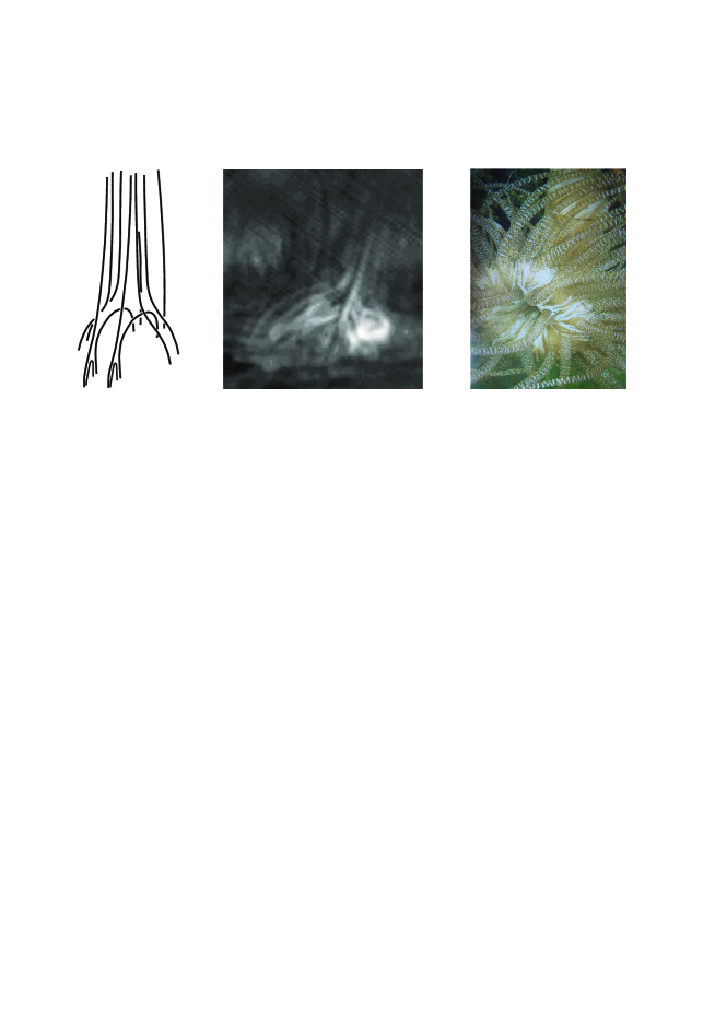
Figure 1: The hypothesized structure of magnetic field lines in the anemone flare [5] (left panel, reprinted with permission from the American Association for the Advancement of Science ©2007) vs. the picture taken by the New Solar Telescope in the Big Bear Solar Observatory [6] (middle panel, reprinted with permission from the American Astronomical Society ©2016), as well as an example of the biological anemone (right panel, courteously provided by G.A. Porfir’eva).

On the other hand, a much more sophisticated topology can be realized in the so-called anemone microflares, occurring in the solar chromosphere (i.e., a bit above the photosphere). The first hints to this phenomenon were given by observations of Hinode satellite [5]. Namely, a few diverging small-scale luminous ribbons were found in the base of such flares. Then, they were qualitatively interpreted as footpoints of the magnetic field lines experiencing the bifurcations (branching) at some height in the course of magnetic reconnection (left panel in Fig. 1). A decade later, such bifurcations became directly observable by the New Solar Telescope in the Big Bear Solar Observatory (California, USA) [6]; a particular example is presented in the middle panel of Fig. 1. At last, the right panel of this figure illustrates a remarkable similarity of such flares with the sea anemone, which are well known in biology.

A theoretical interpretation of the above-mentioned phenomenon requires a consideration of bifurcations of the solar magnetic fields, for example, in the framework of the potential field model formed by the effective point-like charges.

1.1 The Concept of the Effective Magnetic Charges

Since both the present paper and a number of previous studies on the topology of solar magnetic fields were substantially based on the idea of the effective magnetic charges, it it reasonable to explain this concept in more detail. Strictly speaking, any magnetic field is non-divergent (${\rm div}\,{\bf B}=0$). Therefore, its field lines are closed, and there cannot exist any magnetic charges (sources and sinks). However, it is often convenient to introduce the “effective” magnetic charges in the sense illustrated in Fig. 2.

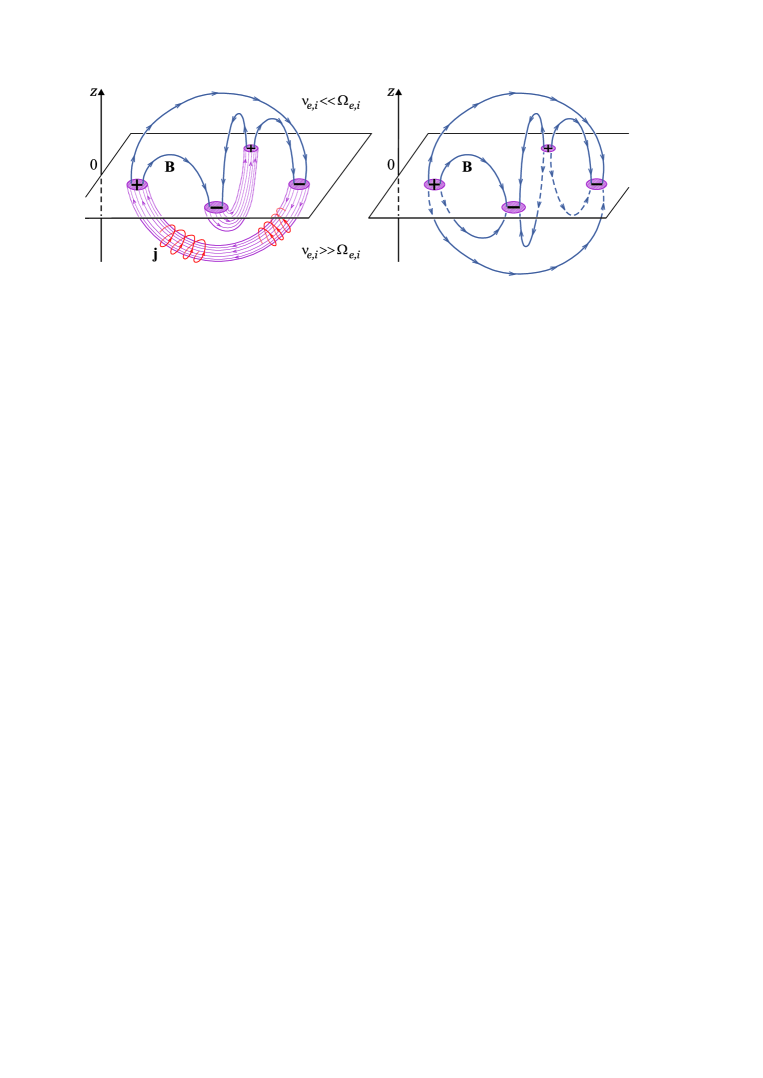
Figure 2: Magnetic-field sources and sinks in the solar atmosphere, caused by the open ends of the magnetic-flux tubes under the photosphere (left panel), and their formal reduction to the magnetic charges (positive and negative, respectively) in the plane $z\,=\,0$ (right panel).

Namely, the electric currents ${\bf j}$ in the deep layers of the Sun (where the collisional frequencies of both electrons and ions are much greater than their gyrofrequencies, ${{\nu}_{e,i}}\,{\gg}\,{{\Omega}_{e,i}}$) form the tubes of the concentrated magnetic flux. The open ends of such tubes at the surface of photosphere, $z=0$, serve as the sources and sinks of the magnetic field in the upper layers of the Sun, which are collisionless, ${{\nu}_{e,i}}\,{\ll}\,{{\Omega}_{e,i}}$ (left panel in Fig. 2). Moreover, in certain circumstances, this magnetic field is approximately current-free, i.e., potential (${\rm rot}\,{\bf B}=0$).

Next, one can consider only the upper semispace (${z}\,{\geq}\,{0}$) and formally perform its mirror reflection with respect to the plane ${z}\,{=}\,{0}$ (right panel in the same figure). As a result, we get a symmetric pattern of the magnetic-field lines, whose sources and sinks (the effective “magnetic charges”) are located exactly in the plane ${z}\,{=}\,{0}$. Therefore, as was pictorially outlined in paper [7], “magnetic field enters the corona from the interior of the Sun through isolated magnetic features on the solar surface. These features correspond to the tops of submerged magnetic flux tubes, and coronal field lines often connect one flux tube to another, defining a pattern of inter-linkage. Using a model field, in which flux tubes are represented as point magnetic charges, it is possible to quantify this inter-linkage.”

The potential field generated by the set of charges (monopoles) is similar to the electrostatic field, and it is quite convenient for the subsequent mathematical analysis. Of course, some care must be taken in the interpretation of the corresponding mathematical results. For example, if one have found some number of peculiarities of the field (e.g., null points) beyond the plane ${z}\,{=}\,{0}$, then only one half of them will have a real physical meaning (namely, those located in the upper semispace). On the other hand, if such peculiarities are localized exactly in the plane ${z}\,{=}\,{0}$, then all of them should be treated as physically relevant.

1.2 Review of the Previous Studies

While the term “topology of magnetic field” is widely employed in the literature on solar physics, there were actually a very few papers devoted to the rigorous topological analysis of the respective magnetic configurations. They were usually based on the computer simulations supplemented by some analytical results from the algebraic topology. One of the first works of this kind was paper [8], whose authors analyzed a few particular configurations of the magnetic field produced by the four magnetic charges (two positive and two negative) with equal magnitudes. A much more general analysis of approximately the same situation was performed in paper [9], where four magnetic charges were allowed to be arbitrary located in the plane of the photosphere. Next, employing some theorems of differential geometry and algebraic topology, the authors established the general criteria for the existence of null points of various types (both in and out of the plane of charges) depending on the localization of the charges. The most interesting finding was that there are such positions of the magnetic charges when a tiny displacement of one of them results in the emergence of a new null point and its fast motion over a considerable distance high above the plane of the sources. This fact inspired a new mechanism of the magnetic reconnection, the so-called “topological trigger” [10]; examples of its practical application to the particular flares can be found, e.g., in paper [11].

Next, bifurcations of the null points in the systems formed by three and four unbalanced irregularly-located charges were analyzed in paper [12]. On the other hand, paper [13] dealt with a highly-symmetric configuration: the numerous positive magnetic charges (sources) were localized in the nodes of a hexagonal network (mimicking the so-called supergranule convective cells) and a single negative charge (sink) was placed in the center of this structure. Then, the authors sought for the null points both in and above the plane of the charges, as well as studied their emergence and displacement depending on the magnitude of the central sink and its shift from the center of symmetry. A further discussion of both symmetric and irregular magnetic-charge configurations with special emphasis on the emergence of the “off-plane” null points was given in paper [14]. Review of application of various topological methods in the solar physics can be found in paper [15].

As follows from the above discussion, the previous works treated either configurations with rather symmetric arrangement or very small number of the magnetic charges. On the other hand, in view of the recent interest to the anemone (branching) solar flares, it would be important to get criteria for the emergence of null points when the magnetic charges are numerous and located irregularly. So, it is the aim of the present paper to perform such analysis by using the Morse–Smale theory of vector fields.

2 Summary of the main results

The magnetic charge is called positive if the field flux through an arbitrary small sphere covering the charge is positive. The negative charge is defined by a similar way: the field flux through an arbitrary small sphere covering such a charge is negative.

The group of charges $\mathcal{C}$ is called positively unbalanced if it can be embedded into the ball $B$ so that the magnetic field is directed outwards at its boundary. The above-specified ball $B=B(\mathcal{C})$ will be called a source region of the group $\mathcal{C}$. The negatively unbalanced group of charges is defined by a similar way, and it is associated with a sink region of the group.

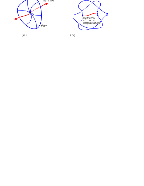
Figure 3: Structure of the null point (a) and the heteroclinic separator (b).

The idealized magnetic charge corresponds to a point-like singularity in the vector field; the positive charge being considered as a source and the negative charge as a sink of the field. The point $p_{0}$ of the magnetic field ${\bf B}$ is called the null point if ${\bf B}(p_{0})=0$. The eigenvalues ${\lambda}_{1}$, ${\lambda}_{2}$ and ${\lambda}_{3}$ in the null point are typically nonzero and satisfy the equality ${\lambda}_{1}+{\lambda}_{2}+{\lambda}_{3}=0$, because ${\nabla}{\cdot}{\bf B}=0$. Consequently, from the viewpoint of the theory of dynamical systems, the null point is a conservative saddle, possessing one 1D and one 2D separatrices; see figure 3(a). If the magnetic field line on the 1D separatrix is directed from the null point, then all field lines on the 2D separatrix surface are directed to the null point; and vice versa.

The following two cases are possible for a typical null point $p_{0}$ (up to redefinition of the eigenvalues):
(1) ${\lambda}_{1}>0$,  ${\lambda}_{2},{\lambda}_{3}<0$;
(2) ${\lambda}_{1}<0$,  ${\lambda}_{2},{\lambda}_{3}>0$.

In the first case, the null point $p_{0}$ is called positive, because ${\lambda}_{1}{\cdot}{\lambda}_{2}{\cdot}{\lambda}_{3}~{}>~{}0$. From the viewpoint of the theory of dynamical systems, the positive null point represents a saddle with Morse index equal to 1 and topological index equal to $-1$. Such saddle has a 1D unstable separatrix and a 2D stable separatrix. In the second case, the point $p_{0}$ is called negative, because ${\lambda}_{1}{\cdot}{\lambda}_{2}{\cdot}{\lambda}_{3}~{}<~{}0$. Such null point is a saddle with Morse index equal to 2 and topological index equal to $+1$. This saddle has a 1D stable separatrix and 2D unstable separatrix; see Fig. 3(a).

Following the standard terminology [1], the magnetic field line connecting two null points will be called a separator.The separator is called heteroclinic if it represents a transversal intersection of two separatrix surfaces; see Fig. 3(b). Topological structure of the magnetic field is determined by the number and types of the null points, by the location of spines and fans with respect to each other, and by the lines of transversal intersection of the fan surfaces, i.e., the heteroclinic separators. Later on, for simplicity, a separator means the heteroclinic separator.

Theorem 1.

Let a positively unbalanced group $\mathcal{C}$ contain $l\geq 2$ positive charges (and arbitrary number of negative charges). Then there exist at least $l-1$ negative null points in the source region $B(\mathcal{C})$ of this group. If the group $\mathcal{C}$ consists of $l\geq 2$ positive charges and there are exactly $l-1$ null points in $B(\mathcal{C})$, then all these null points are negative and there are no separators in $B(\mathcal{C})$. Moreover, the magnetic field in region $B(\mathcal{C})$ possesses a uniquely defined, up to the topological equivalence, structure.

The next consequences follow from this theorem.

Corollary 1.

Let a negatively unbalanced group $\mathcal{C}$ contain $k\geq 2$ negative charges. Then there exist at least $k-1$ positive null points in the sink region $B(\mathcal{C})$ of this group. If the group $\mathcal{C}$ consists of $k\geq 2$ negative charges and there are exactly $k-1$ null points in $B(\mathcal{C})$, then all these null points are positive and there are no separators in $B(\mathcal{C})$.

Corollary 2.

Let a positively unbalanced group $\mathcal{C}$ contain one (dominant) positive charge and $k\geq 1$ negative charges. Then there exist at least $k$ positive null points in the source region $B(\mathcal{C})$ of this group. If $B(\mathcal{C})$ contains exactly $k$ null points, then all these points are positive and there are no separators in $B(\mathcal{C})$. Moreover, the magnetic field in region $B(\mathcal{C})$ possesses a uniquely defined, up to the topological equivalence, structure.

Corollary 3.

Let a positively unbalanced group $\mathcal{C}$ contains $l\geq 2$ positive and $k\geq 1$ negative charges. Then there exist at least $l-1$ negative null points and at least $k$ positive null points in the source region $B(\mathcal{C})$ of this group.

At the minimal numbers of both the positive and negative null points (which are determined by Corollary 3), the separators can be absent. Nevertheless, as follows from the subsequent theorem, as soon as at least one “excessive” null point appears, at least one separator is inevitably formed. The type of the excessive null point is of no importance: it can be either positive or negative. For the sake of definiteness, we shall consider the case when the excessive point is negative.

Theorem 2.

Let a positively unbalanced group $\mathcal{C}$ contain $l\geq 2$ positive and $k\geq 0$ negative charges. If $B(\mathcal{C})$ contains exactly $l$ negative null points, then there is at least one separator in $B(\mathcal{C})$.

The last theorem demonstrates a particular scenario of emergence of a negative null point, when there is a family of separators whose number is equal to the number of negative null points (and it is equal also to the number of positive charges).

Theorem 3.

Let a positively unbalanced group $\mathcal{C}$ contain $l\geq 2$ positive charges and $l-1$ negative null points, such that this group is defined by the vector field $\vec{F}_{0}$. Then, there is a continuous family of vector fields $\vec{F}_{t}$, $0\leq t\leq 1$, such that the vector field $\vec{F}_{1}$ has $l$ positive charges, $l$ separators, and one negative null point.

3 Auxiliary information

Let $f^{t}$ be a flow induced by the vector field ${\bf V}$ on the 3D sphere $\mathbb{S}^{3}$. We shall assume that $f^{t}$ has no periodic trajectories. Let $Fix~{}(f^{t})$ designate a set of equilibrium states of the flow $f^{t}$. For $p\in Fix~{}(f^{t})$, let $W^{s}(p)$ be a set of trajectories approaching $p$ at infinitely increasing time. In particular, if $p$ is a saddle, then $W^{s}(p)\setminus\{p\}$ is a stable separatrix of the saddle $p$. The set $W^{s}(p)$ is called the stable manifold of the point $p$. Similarly, let $W^{u}(p)$ denote a set of trajectories approaching $p$ at infinitely decreasing time. In particular, if $p$ is a saddle, then $W^{u}(p)\setminus\{p\}$ is an unstable separatrix of the saddle $p$. The set $W^{u}(p)$ is called the unstable manifold of the point $p$. The flow $f^{t}$ is called the Morse–Smale flow if all its equilibrium states are hyperbolic, their stable and unstable manifolds intersect each other transversally, and the limit set for any trajectory belongs to $Fix~{}(f^{t})$. The corresponding vector field ${\bf V}$ is called the Morse–Smale vector field [17].

Let ${\bf v}_{\rm sourse}$ denote the vector field in ball $\mathbb{B}^{3}$ directed outwards at the ball boundary $\partial\mathbb{B}^{3}=S^{2}$ and possessing exactly one source inside the ball. Let us assume that ${\bf v}_{\rm sink}=-{\bf v}_{\rm sourse}$. Obviously, the vector field ${\bf v}_{\rm sink}$ possesses exactly one sink inside the ball $\mathbb{B}^{3}$, and ${\bf v}_{\rm sink}$ is directed inwards the ball $\mathbb{B}^{3}$ at the boundary $S^{2}$.

Let $B(\mathcal{C})$ be the source region of the group of charges $\mathcal{C}$. Let ${\bf v}(\mathcal{C})$ denote the magnetic field in $B(\mathcal{C})$ created by the group $\mathcal{C}$. We remind that the vector field ${\bf v}(\mathcal{C})$ is directed outwards at the boundary $\partial B(\mathcal{C})$ of the ball $B(\mathcal{C})$. If boundaries $\partial\mathbb{B}^{3}=S^{2}$ and $\partial B(\mathcal{C})$ of the balls $\mathbb{B}^{3}$ and $B(\mathcal{C})$, respectively, are identical to each other, then we get a 3D sphere $\mathbb{S}^{3}$. The field ${\bf v}_{\rm sink}$ near the boundary $\partial\mathbb{B}^{3}$ can be corrected so that the fields ${\bf v}_{\rm sink}$ and ${\bf v}(\mathcal{C})$ form a smooth Morse–Smale vector field at $\mathbb{S}^{3}$, which will be denoted by ${\bf V}(\mathcal{C})$. Obviously, a global topological structure of the field ${\bf v}_{\rm sink}$ can be preserved after such transformation. Then the equilibrium states of ${\bf V}(\mathcal{C})$ will represent a union of the equilibrium states for the field ${\bf v}(\mathcal{C})$ and the sink field ${\bf v}_{\rm sink}$. The vector field ${\bf V}(\mathcal{C})$ will be called a continuation of the field ${\bf v}(\mathcal{C})$ by the group $\mathcal{C}$ to the 3D sphere $\mathbb{S}^{3}$.

Lemma 1.

Let a positively unbalanced group $\mathcal{C}$ contain $N^{+}$ (respectively, $N^{-}$) positive (respectively, negative) charges and $S^{+}$ (respectively, $S^{-}$) positive (respectively, negative) null points. Then the following equality is satisfied:

$$1+N^{-}-S^{+}+S^{-}-N^{+}=0.$$ (1)

Proof. Let ${\bf v}(\mathcal{C})$ be the magnetic field in $B(\mathcal{C})$ formed by the group $\mathcal{C}$ and ${\bf V}(\mathcal{C})$ be a continuation of the field ${\bf v}(\mathcal{C})$ to the 3D sphere $\mathbb{S}^{3}$. The charges and null points of the magnetic vector field ${\bf v}(\mathcal{C})$ are the equilibrium states of the Morse–Smale vector field ${\bf V}(\mathcal{C})$. We remind that ${\bf V}(\mathcal{C})$, as compared to ${\bf v}(\mathcal{C})$, has an additional sink whose topological index is equal to unity.

Morse index (dimensionality of the unstable manifold) of the positive null point equals unity. Consequently, the topological index of such a point equals minus unity. Similarly, the topological index of a negative null point equals unity, because its Morse index equals two. Morse index of a negative (respectively, positive) charge equals zero (respectively, three). Therefore, the topological index of a negative (respectively, positive) charge equals unity (respectively, minus unity). As is known, Euler characteristic of 3D sphere equals zero. Using the Euler–Poincaré formula, which states that a sum of topological indices of the equilibrium states is equal to the Euler characteristic, we obtain the required result. $\Box$

Corollary 4.

Let the conditions of lemma 1 be satisfied. If there are no negative charges in the sink region ($N^{-}=0$), then

$$S^{-}=(N^{+}-1)+S^{+}\geq N^{+}-1.$$

Let us introduce the partial order $\prec$ in the set of equilibrium states $Fix~{}(f^{t})$ of the flow $f^{t}$. For $p,q\in Fix~{}(f^{t})$, let us define that $p\prec q$ if $W^{s}(p)\cap W^{u}(q)\neq\emptyset$. It is convenient to present the above order in the graph whose points are identified with the equilibrium states $Fix~{}(f^{t})$. The graph vertices corresponding to $p,q\in Fix~{}(f^{t})$ and related by the order $p\prec q$ are connected by the arc directed from $q$ to the point $p$. Such a directed graph $\Gamma(f^{t})$ is sometimes called Smale graph (or diagram).

Let us denote a union of all unstable 1D manifolds of the saddles and all sinks of the flow $f^{t}$ by $A(f^{t})$. It is known [18] that $A(f^{t})$ is a connected 1D subgraph of the graph $\Gamma(f^{t})$, whose vertices are identified with the respective saddles and sinks. In this case, arcs of the subgraph correspond to the 1D unstable separatrices, and they are supplied with the directions from the saddles to sinks. Moreover, $A(f^{t})$ is the attracting set of the flow $f^{t}$ [18]. Similarly, let us denote a union of all stable 1D separatrices of the saddles and all sources by $R(f^{t})$. Then, $R(f^{t})$ is a connected oriented subgraph, which is a repelling set of the flow $f^{t}$ [18].

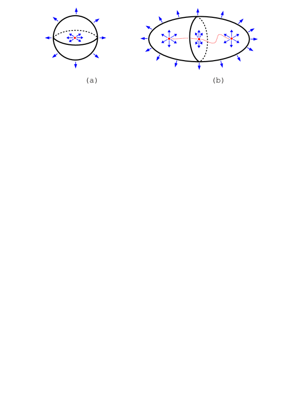
Figure 4: Vector field ${\bf v}_{\rm sourse}$ (a) and vector field ${\bf v}_{\rm uns}$ of type (2; 1) in the ball $\mathbb{B}^{3}$ (b).

To describe a topological structure of the vector fields, we need some canonical fields. The vector field ${\bf v}_{\rm sourse}$ will be called the source of type (1; 0). Let us consider the vector field ${\bf v}_{\rm uns}$ in the ball $\mathbb{B}^{3}$ directed outwards at the ball boundary $\partial\mathbb{B}^{3}=S^{2}$ and possessing $l\geq 2$ sources ${\alpha}_{1},\ldots,{\alpha}_{l}$ and $l-1$ saddles ${\sigma}_{1},\ldots,{\sigma}_{l-1}$ with Morse index 2. Such vector field ${\bf v}_{\rm uns}$ will be called the source of type (l; l–1). Structure of the vector field of type (2; 1) is shown in Fig. 4(b). The vector field ${\bf v}_{\rm sourse}$ can be treated as the source of type (1; 0), as illustrated in Fig. 4(a).

Let as assume that ${\bf v}_{\rm sink}=-{\bf v}_{\rm sourse}$ and ${\bf v}_{\rm stab}=-{\bf v}_{\rm uns}$. The vector field ${\bf v}_{\rm sink}$ is directed inwards at the ball boundary $\partial\mathbb{B}^{3}=S^{2}$ and has one sink inside the ball $\mathbb{B}^{3}$. The vector field ${\bf v}_{\rm stab}$ is directed inwards at the ball boundary $\partial\mathbb{B}^{3}=S^{2}$ and has $l\geq 2$ sinks ${\omega}_{1},\ldots,{\omega}_{l}$ and $l\!-\!1$ saddles with Morse index 1. Such vector field ${\bf v}_{\rm uns}$ will be called the sink of type (l ; l –1). Without loss of generality we can assume that the above-mentioned vector fields are orthogonal to the boundary $\partial\mathbb{B}^{3}=S^{2}$ and are unitary at this boundary.

If boundaries of two copies of the ball $\mathbb{B}^{3}$ are identified with each other, then we get a 3-sphere $\mathbb{S}^{3}$. If a source of the type ($l\,$; $l\,$–1) is defined in one copy of the ball, and the field ${\bf v}_{\rm sink}$ is defined in another copy of the ball, then we get a smooth vector field in $\mathbb{S}^{3}$, which will be denoted by ${\bf V}_{\rm uns}(l;l\!-\!1)$. In fact, the following statement follows from the works [18] and [19]:

Proposition 1.

Let the Morse–Smale vector field ${\bf V}$ be defined in the 3D sphere $\mathbb{S}^{3}$ and its nonwandering set be composed of $l\geq 2$ sources, $l-1$ saddles of Morse index 2 and one sink. Then ${\bf V}$ is topologically equivalent to ${\bf V}_{\rm uns}(l;l-1)$.

Proof. Let $f^{t}$ denote the Morse–Smale flow generated by the vector field ${\bf V}$. Since the number of sources is greater than the number of saddles of Morse index 2 by unity, then the attractive set $A(f^{t})$ is a segment with sinks and saddles. Moreover, the saddles and sinks occur alternatively, and the endpoints of segment $A(f^{t})$ are the sources. Following Lemma 1.1 [19], the set $A(f^{t})$ has a ball neighborhood that is the source of type $(l;l-1)$. There is a sink beyond this neighborhood. This leads to the required result. $\Box$

4 Proofs of the main results

Proof of Theorem 1. Let ${\bf v}(\mathcal{C})$ be the magnetic field in $B(\mathcal{C})$ formed by the group $\mathcal{C}$ and ${\bf V}(\mathcal{C})$ be a continuation of the field ${\bf v}(\mathcal{C})$ to the 3D sphere $\mathbb{S}^{3}$. Therefore, the field ${\bf V}(\mathcal{C})$ has an additional sink as compared to ${\bf v}(\mathcal{C})$. We need to prove the inequality $S^{-}\geq l-1$, where $S^{-}$ is the number of negative null points of the vector field ${\bf V}(\mathcal{C})$. Let us prove this inequality by the method of mathematical induction where the inductive step is done by the number $l=N^{+}$ of the positive charges (which is equal to the number of sources of the field ${\bf V}(\mathcal{C})$). We remind that ${\bf V}(\mathcal{C})$ is the Morse–Smale vector field, which induces the Morse–Smale flow $f^{t}$ in $\mathbb{S}^{3}$.

Firstly, we show that there exists at least one negative null point for any $l\geq 2$ (this will be simultaneously a proof of the initial step at $l=2$). Let $A=A(f^{t})$ be a union of all sinks and unstable (1D) separatrices of all the saddles of Morse index 1. Let us assume that the above statement is false. Then the complement of $A$ is a union of the nonintersecting unstable (3D) manifolds of $l\geq 2$ sources. Since a complement of the 1D graph $A$ is a connected set, then we get a contradiction to the connectivity of the set $\mathbb{S}^{3}{\setminus}A$.

Let us assume that the statement is proved for the number of sources $2,\ldots,l\geq 2$ and show that it will be true for $l+1\geq 3$. As follows from the previous discussion, there exists at least one saddle $\sigma$ with Morse index 2. Two (1D) stable separatrices $Sep^{s}_{1}$ and $Sep^{s}_{2}$ of the saddle $\sigma$ belong to the unstable manifolds of the sources ${\alpha}_{1}$ and ${\alpha}_{2}$, respectively. Let us consider two cases: (1) ${\alpha}_{1}\neq{\alpha}_{2}$ and (2) ${\alpha}_{1}={\alpha}_{2}$. In the first case, the set ${\alpha}_{1}\cup Sep^{s}_{1}\cup\sigma\cup Sep^{s}_{2}\cup{\alpha}_{2}=S$ is a repelling set. It follows from ${\alpha}_{1}\neq{\alpha}_{2}$ that this set $S$ has a neighborhood homeomorphic to a 3-ball, which looks like the source. Then the original flow can be replaced by the flow with one source instead of two sources ${\alpha}_{1}$, ${\alpha}_{2}$ and the saddle $\sigma$. The resulting flow satisfies the inductive assumption. Since this flow has exactly one source and one saddle less than before, we get the required estimate for the original flow. As follows from the above argumentation, if there exists a saddle with Morse index 2 for which case (1) is realized, then the inequality $S^{-}\geq l-1$ is proved.

In the second case, when ${\alpha}_{1}={\alpha}_{2}$, without loss of generality we can believe that this case is realized for all the saddles with Morse index 2. Then each such saddle is uniquely associated with a source, $\sigma\mapsto\alpha={\alpha}_{1}={\alpha}_{2}$. As a result, we get a stronger inequality $S^{-}{\geq}\,l$.

Therefore, the inequality $S^{-}\geq l-1$ is proved for any group of charges containing $l\geq 2$ positive charges. We note that if there are no negative charges in the group, then $N^{+}=l$ and $N^{-}=0$, and consequently the inequality $S^{-}\geq l-1$ follows from Corollary 4.

If $S^{-}=l-1$, then formula (1) leads to $S^{+}=0$, and consequently all the null points are negative. Therefore, there are no separators in $B(\mathcal{C})$.

Uniqueness of the topological structure follows immediately from Proposition 1. $\Box$

Proof of Theorem 2. Let ${\bf v}(\mathcal{C})$ be the vector field in $B(\mathcal{C})$ formed by the group $\mathcal{C}$ and ${\bf V}(\mathcal{C})$ be a continuation of the field ${\bf v}(\mathcal{C})$ to the 3D sphere $\mathbb{S}^{3}$. It is specified that ${N^{+}}\!=l$, ${S^{-}}\!=l$ and ${N^{-}}\!=0$. Then formula (1) leads to ${S^{+}}\!=1$. Let ${\sigma}_{0}$ denote the single saddle with topological index minus one.

Let $f^{t}$ be the Morse–Smale flow generated by the vector field ${\bf V}(\mathcal{C})$ in the 3D sphere $\mathbb{S}^{3}$. We consider the connected 1D graph $R(f^{t})$ composed of all 1D stable manifolds of the saddles and all sources of the flow $f^{t}$. Let us remind that $R(f^{t})$ is a repelling set of the flow $f^{t}$.

Proposition 2.

The graph $R(f^{t})$ has the neighborhood $U(R)$ possessing the following properties:

• the boundary $\partial U(R)$ of the neighborhood $U(R)$ is transversal to the flow $f^{t}$, and trajectories of the flow leave $U(R)$ with increasing time;

• the neighborhood $U(R)$ is homeomorphic to a solid torus (consequently, the boundary $\partial U(R)$ is homeomorphic to 2D torus);

• there exists the saddle $\sigma\in U(R)$ (the negative null point) whose 2D unstable separatrix $W^{u}(\sigma)$ intersects the torus $\partial U(R)$ along a closed curve homotopic to the null meridian of the torus $\partial U(R)$.

Proof of Proposition 2. According to our conditions, vertices of the graph $R(f^{t})$ are composed of $l$ saddle and $l$ source points; so that exactly two arcs enter the each saddle point, and at least one arc leaves the each source point. Then $R(f^{t})$ contains the simple cycle $C$ of type (2; 3), which is supplemented by some (probably, zero) number of segments; each of these segments contains the equal numbers of source and saddle points (which equal the number of arcs in the segment). The cycle $C$ has a neighborhood that is homeomorphic to a solid torus; and the trajectories leave it with increasing time, because $C$ possesses the type (2; 3). Without loss of generality we can believe that there is no sink in this neighborhood (otherwise, the neighborhood can be decreased). Each of the attached segments has a neighborhood homeomorphic to a ball, and the trajectories leave this ball with increasing time. Consequently, there exist the required neighborhood $U(R)$ without a sink. Since $C$ contains at least one saddle, its 2D unstable separatrix must intersect $\partial U(R)$ along a closed curve homeomorphic to meridian of the torus. So, Proposition 2 is proved. $\diamondsuit$

Note that the graph $A(f^{t})$, which is an attracting set of the flow $f^{t}$, represents a simple cycle composed of the sink ${\omega}_{0}$, saddle ${\sigma}_{0}$ and two its 1D unstable separatrices. Consequently, $A(f^{t})$ has the neighborhood $U(A)$ homeomorphic to a solid torus, so that its boundary $\partial U(A)$ is transversal to the flow $f^{t}$, and the trajectories enter $U(A)$ with increasing time. For the sufficiently small neighborhood $U(A)$, a 2D stable separatrix of the saddle ${\sigma}_{0}$ intersects the 2D torus $\partial U(A)$ along a closed simple curve homotopic to a meridian of the torus $\partial U(A)$. Let this curve be denoted by ${\mu}_{0}$.

Without loss of generality we can believe that the neighborhoods $U(R)$ and $U(A)$ do not intersect each other. Since their union contains all equilibrium states of the flow $f^{t}$, any positive semitrajectory with the initial point at $\partial U(R)$ must intersect the torus $\partial U(A)$. Consequently, the sphere $\mathbb{S}^{3}$ can be presented as two solid tori $U(R)$ and $U(A)$ where their boundaries $\partial U(R)$ and $\partial U(A)$ are matched to each other. Let $\vartheta:\partial U(A)\to\partial U(R)$ be such homeomorphism that $\mathbb{S}^{3}=U(A){\bigcup}_{\vartheta}U(R)$. As is known, a gluing of two solid tori results in a 3-sphere only when a meridian in one boundary torus is matched to the parallel (which may be rotated a few times along the meridian) in another boundary torus. Consequently, the image of curve ${\mu}_{0}$ with respect to $\vartheta$ is a closed curve, which intersects any closed curve at $\partial U(R)$ homotopic to the null meridian of the torus $\partial U(R)$. Consequently, there exists at least one separator. $\Box$

The proof of Proposition 2 immediately leads to the following statement, which will be used later.

Proposition 3.

Let the premises of Theorem 2 be satisfied, and let $f^{t}$ be the Morse–Smale flow generated by the vector field ${\bf V}(\mathcal{C})$ in the 3D sphere $\mathbb{S}^{3}$, which is a continuation of the magnetic field in $B(\mathcal{C})$. Let us assume that the graph $A(f^{t})$ is a simple closed curve. Then there exit at least $l$ separators in $B(\mathcal{C})$.

Proof. In designations of Proposition 2 we get that the unstable 2D separatrix of each saddle from $\partial U(R)$ intersects $\partial U(R)$ along a closed curve homotopic to null meridian of the torus $\partial U(R)$. Since $\partial U(R)$ contains $l$ saddles, there exist at least $l$ separators. $\diamondsuit$

Proof of Theorem 3. For the sake of simplicity, we construct the required family for $l=2$. As will be seen from our discussion, such family can be constructed with an arbitrary number $l\geq 2$ of the positive charges.

We consider the Euclidean space $\mathbb{R}^{3}$ endowed with the cylindrical coordinates $(\varrho;\varphi;z)$ and Cartesian coordinates $(x,y,z)$. Let $U_{1}$ be the neighbourhood of the origin $(0,0,0)$ defined by $|x|<0.9$, $|y|<0.9$, $|z|<1$, and $U$ the neighbourhood defined by $|x|<\frac{1}{2}$, $|y|<\frac{1}{2}$, $|z|<\frac{1}{2}$. Outside of $U_{1}$, the vector field $\vec{F}_{0}$ is described by the following system:

$$\dot{\varrho} = \varrho\cdot\left[\varrho-1+4\Psi(\varphi)\right],$$ (2)

$$\dot{\varphi} = -\sin(2\varphi),$$ (3)

$$\dot{z} = z,$$ (4)

where

$$\Psi(\varphi)=\sin^{2}\left(\frac{\varphi-\frac{\pi}{2}}{2}\right)\sin^{2}\left(\frac{\varphi-\pi}{2}\right)\sin^{2}\left(\frac{\varphi-\frac{3\pi}{2}}{2}\right).$$

The vector field $\vec{F}_{0}$ can be extended in the neighbourhood $U$ so that $\vec{F}_{0}$ is described by the following system:

$$\left\{\begin{array}[]{ccl}\dot{x}&=&1,\\ \dot{y}&=&-y,\\ \dot{z}&=&z.\\ \end{array}\right.$$

Note that ${\rm div}\,\vec{F}_{0}|_{U}\equiv 0$.

All equilibrium states of $\vec{F}_{0}$ are in the plane $z=0$, which is a repeller for the vector field defined by this system. Since the set of equations can be split into the first two equations (2), (3) and the third equation (4), it is sufficient to consider a phase portrait in the plane $z=0$. The equilibrium states in this plane can be only at the rays $\varphi=0$, $\varphi=\frac{\pi}{2}$, $\varphi=\pi$, and $\varphi=\frac{3\pi}{2}$.

Then, equation (2) takes the form:

$$\dot{\varrho}=\left\{\begin{array}[]{lcl}\varrho^{2}&\mbox{at}&\varphi=0,\;\varrho\neq 0,\\ \varrho\,(\varrho-1)&\mbox{at}&\varphi\in\{\frac{\pi}{2},\pi,\frac{3\pi}{2}\},\;\varrho\neq 0.\end{array}\right.$$

Consequently, there are three equilibrium states: $O_{2}(1;\frac{\pi}{2})$ is a source, $O_{3}(1;\pi)$ is a saddle, and $O_{4}(1;\frac{3\pi}{2})$ is a source; see Fig. 5(a). The saddle $O_{3}(1;\pi)$ in space has the Morse index 2. The calculations show that ${\rm div}\,\vec{F}_{0}(O_{3})=0$.

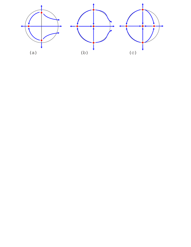
Figure 5: Phase portrait in the plane $z=0$.

Now, starting with $\vec{F}_{0}$, we shall construct the family of vector fields $\vec{F}_{t}$ keeping $\vec{F}_{t}=\vec{F}_{0}$ outside of $U_{1}$ and deforming $\vec{F}_{0}$ near the origin $(0,0,0)$ in Cartesian coordinates $(x,y,z)$. First, the family $\vec{F}_{\nu}$, $0\leq\nu\leq 1$, described by the system

$$\left\{\begin{array}[]{ccl}\dot{x}&=&(\nu-1)^{2}+\nu^{2}x^{2},\\ \dot{y}&=&-y,\\ \dot{z}&=&z(1-2\nu x)\\ \end{array}\right.$$

moves $\vec{F}_{0}$ into the vector field $\vec{F}_{\nu=1}$ defined by the system

$$\left\{\begin{array}[]{ccl}\dot{x}&=&x^{2},\\ \dot{y}&=&-y,\\ \dot{z}&=&z(1-2x).\\ \end{array}\right.$$

Easy calculations show that ${\rm div}\,\vec{F}_{\nu}\equiv 0$ for any $0\leq\nu\leq 1$. So, the saddle–node $O_{0}(0;0)$ in the origin of coordinates is added to the previous equilibrium states $O_{2}(0;1)$, $O_{3}(-1;0)$, and $O_{4}(0;-1)$; see Fig. 5(b). It is convenient to denote $\vec{F}_{\nu=1}$ by $\vec{F}_{0}$ again.

At last, let us consider the family $\vec{F}_{\mu}$, $0\leq\mu\leq\frac{1}{3}$, of vector fields defined by the system:

$$\left\{\begin{array}[]{ccl}\dot{x}&=&-\mu x+x^{2},\\ \dot{y}&=&-y,\\ \dot{z}&=&z(1+\mu-2x).\\ \end{array}\right.$$

Again, it is easy to see that ${\rm div}\,\vec{F}_{\mu}\equiv 0$ for any $0\leq\mu\leq\frac{1}{3}$. Consequently, the saddle–node $O_{0}(0;0)$ in the plane $(x;y)$ decays into the sink $O_{0}(0;0)$ and saddle $O_{1}(\frac{1}{3};0)$; see Fig. 5(c). Therefore, two separators are formed. $\Box$

5 Discussion and Conclusions

1. Using the Morse–Smale theory, we derived a set of constraints on the number of the magnetic-field sources (the effective “magnetic charges”) and the null points of various types (positive and negative), which should be a valuable tool for analyzing the structure of complex magnetic fields, particularly, in the solar anemone flares. On the one hand, the formulas presented in Sections 2–4 are less powerful than the ones derived in the old paper [9], because they are based on the purely topological consideration and, therefore, do not specify any relations between the positions of the magnetic charges and null points. On the other hand, these formulas are more general than the previously-known ones, because they are applicable to the arbitrary number of the charges. In particular, we present configurations of the charges and null points of a given type such that no separators exist. (This does not mean that the given type of the group forbids the existence of separators.)

2. An important prerequisite for application of the Morse–Smale inequalities is the requirement that the group of the magnetic charges is positively (or negatively) unbalanced, as defined in Section 2. Of course, this narrows the scope of applicability of the above-mentioned inequalities to the particular configurations of solar magnetic fields. However, as was demonstrated in the recent observational work [20], the anemone microflares often develop in the regions with unbalanced magnetic polarity. So, the applicability of the Morse–Smale constraints to the these cases is well justified.

3. At last, attention should be paid to the correct physical interpretation of our mathematical constraints. Namely, as follows from the discussion in Section 1.1, if $S^{\pm}_{\rm in}$ is the number of “physical” null points in the plane of magnetic charges and $S^{\pm}_{\rm out}$ is their number out of this plane, then $S^{\pm}=S^{\pm}_{\rm in}+2S^{\pm}_{\rm out}$. On the other hand, all magnetic charges should be taken with the coefficient of unity, because in all physically-relevant situations they must be localized in the same plane.

References

- [1] E. Priest, T. Forbes, Magnetic Reconnection: MHD Theory and Applications, Cambridge Univ. Press, Cambridge, UK, 2000.
- [2] B. Somov, Plasma Astrophysics, Part II: Reconnection and Flares, 2nd Edition, Springer, NY, 2013.
- [3] G. Huang, V. Melnikov, H. Ji, Z. Ning, Solar Flare Loops: Observations and Interpretations, Springer, Singapore, 2018.
- [4] I. Nikulin, Y. Dumin, Coronal partings, Adv. Space Res. 57 (2016) 904.
- [5] K. Shibata, T. Nakamura, T. Matsumoto, K. Otsuji, T. Okamoto, et al., Chromospheric anemone jets as evidence of ubiquitous reconnection, Science 318 (2007) 1591.
- [6] Z. Zeng, B. Chen, H. Ji, P. Goode, W. Cao, Resolving the fan-spine reconnection geometry of a small-scale chromospheric jet event with the New Solar Telescope, Astrophys. J. Lett. 819 (2016) L3.
- [7] D. Longcope, Topology and current ribbons: A model for current, reconnection and flaring in a complex, evolving corona, Solar Phys. 169 (1996) 91.
- [8] P. Baum, A. Bratenahl, Flux linkages of bipolar sunspot groups: A computer study, Solar Phys. 67 (1980) 245.
- [9] V. Gorbachev, S. Kel’ner, B. Somov, A. Shvarts, A new topological approach to the question of the trigger for solar flares, Soviet Astron. 32 (1988) 308.
- [10] B. Somov, On the topological trigger of large eruptive solar flares, Astron. Lett. 34 (2008) 635.
- [11] A. Oreshina, I. Oreshina, B. Somov, Magnetic-topology evolution in NOAA AR 10501 on 2003 November 18, Astron. & Astrophys. 538 (2012) A138.
- [12] D. Brown, E. Priest, The topological behaviour of stable magnetic separators, Solar Phys. 190 (1999) 25.
- [13] G. Inverarity, E. Priest, Magnetic null points due to multiple sources of solar photospheric flux, Solar Phys. 186 (1999) 99.
- [14] D. Brown, E. Priest, The topological behaviour of 3D null points in the Sun’s corona, Astron. & Astrophys. 367 (2001) 339.
- [15] D. Longcope, Topological methods for the analysis of solar magnetic fields, Liv. Rev. Sol. Phys. 2 (2005) 7.
- [16] V. Grines, T. Medvedev, O. Pochinka, E. Zhuzhoma, On heteroclinic separators of magnetic fields in electrically conducting fluids, Physica D 294 (2015) 1.
- [17] S. Smale, Differentiable dynamical systems, Bull. Amer. Math. Soc. 73 (1967) 747.
- [18] V. Grines, E. Zhuzhoma, V. Medvedev, O. Pochinka, Global attractor and repeller of Morse–Smale diffeomorphisms, Proc. Steklov Inst. Math. 271 (2010) 103.
- [19] S. Pilyugin, On topological equivalence of rough three-dimensional systems without periodic trajectories, Diff. Equat. 11 (1975) 1375, in Russian.
- [20] Y. Dumin, B. Somov, New types of the chromospheric anemone microflares: Case study, Solar Phys. 295 (2020) 92.