Time-linear scaling NEGF method for real-time simulations of interacting electrons and bosons. II. Dynamics of polarons and doublons

Abstract

Nonequilibrium dynamics of the open chain Holstein-Hubbard model is studied using the linear time-scaling GKBA+ODE scheme developed in the preceeding paper. We focus on the set of parameters relevant for photovoltaic materials, i. e., a pair of electrons interacting with phonons at the cross-over between the adiabatic and anti-adiabatic regimes and at moderately large electron-electron interaction. By comparing with exact solutions for two corner cases, we demonstrate the accuracy of the $T$-matrix (in the $pp$ channel) and the second-order Fan ($GD$) approximations for the treatment of electronic ($e$-$e$) and electron-phonon ($e$-ph) correlations, respectively. The feedback of electron on phonons is consistently included and is shown to be mandatory for the total energy conservation. When two interactions are simultaneously present, our simulations offer a glimpse into the dynamics of doublons and polarons unveiling the formation, propagation and decay of these quasiparticles, energy redistribution between them and self-trapping of electrons.

I Introduction

Even in the absence of $e$-$e$ interactions, electrons coupled to bosons represent one of the most studied systems in physics [1, 2, 3]. Restricting to solid state and molecular physics, there are numerous models of increasing complexity: a core electron coupled to plasmons [4, 5, 6], the Holstein dimer [7, 8] or a quantum dot coupled to leads [9, 10, 11, 12, 13, 14, 15] as a paradigmatic model for the Franck-Condon blockade in nanoscale transport, and infinite 1D and 2D systems at various fillings representing phenomena ranging from the energy transfer along conjugated polymer chains and photovoltaic devices [16, 17], the oscillations in the excitonic condensate in transition metal di- and ternary-chalcogenides [18], to correlated cuprate systems [19, 20]. A common physical phenomenon pertinent to all of them is the emergence of a new kind of quasiparticle — the polaron — an electron surrounded by a cloud of coherent phonons [21].

Historically, one-dimensional coordination polymers [22] were among the first systems where $e$-ph dynamics have been studied experimentally [23, 24] and theoretically [25], and a good understanding of polaron formation and localization has been obtained. In fact, they are convenient paradigmatic materials for theoretical NEGF investigations. They can be characterized by a small set of parameters, and the 1D nature makes them amenable to alternative theoretical methods, including the wave-function [25, 26, 27, 28], the density-matrix renormalization group [29], the hierarchical equations of motion [16] and matrix product state [30, 31] based ones. Much more versatile and practically relevant are materials for photovoltaic applications [32]. By the very nature of solar energy conversion, several crucial aspects — creation of nonequilibrium carriers, their dressing and formation of the polaronic quasiparticles, and transport through the active material to electrodes — creates a good predisposition for a NEGF theory and poses very interesting challenges, e. g., simulation of picosecond (ps) polaron self-localization in $\alpha$-Fe₂O₃ photoelectrochemical cells [33].

We are close to achieving the goal of ps dynamics within a NEGF theory: $e$-ph thermalization has already been demonstrated in a model insulator without $e$-$e$ interactions on a 2 ps time-scale [34], whereas $e$-$e$ interacting 2D systems have been propagated for 100 fs [35]. Here, we illustrate our methods by applying them to electron-phonon ($e$-ph) dynamics in the 1D Holstein-Hubbard model [36, 30]. The model features important physical mechanisms present in realistic systems and enables us to benchmark the GKBA+ODE scheme of the real-time NEGF theory in complicated cross-over regimes.

The outline of our work is as follows. After recapitulating basic ingredients of the NEGF formalism (see paper I for the full-fledged theory) in Section II, we introduce the open-chain Holstein-Hubbard model in Section III. Numerical scaling with the system dimension and strategies for code optimization are discussed and compared with alternative approaches. More insights into the model dynamics are obtained in the partial cases where only $e$-$e$ or $e$-ph interaction is present. Therefore, in Sec. IV we provide benchmarks against numerically exact solutions of the Hubbard model. Besides finding a high level of accuracy of the $T$-matrix approximation in the particle-particle channel, it is shown that doublons play an important role in the system dynamics. In Sec. V the concept of polaron is introduced and results for the electron localization in the Holstein model are presented. Then, we discuss how electrons and doublons propagate when $e$-$e$ and $e$-ph are simultaneously present (Sec. VI) at the level of $T$-matrix and the fully dressed second-order Fan ($GD$) approximation. We find that $e$-ph interactions modify the localization of doublons in a nontrivial way. We discuss two competing mechanisms and support our interpretation by analyzing total energy contributions and $e$-ph correlators. Conclusions and outlook are drawn in Section VII.

II Electron-boson NEGF equations

The theory developed in the preceding paper I is completely general and can be applied to a wide range of physical systems out of equilibrium with electron-electron and electron-boson interactions. Here we consider specifically electrons interacting with phonons as one of the most interesting and technologically relevant cases. Henceforth we use latin letters to denote one-electron states; thus $i\equiv(\bm{i},\sigma)$ is a composite index standing for an orbital degree of freedom $\bm{i}$ and a spin projection $\sigma$. For phonons, one may work with standard creation and annihilation operators $\hat{a}_{\bm{\mu}}^{\dagger}$ and $\hat{a}_{\bm{\mu}}$ for the mode $\bm{\mu}$, respectively. However, since electrons typically couple to the phononic displacement, it is of advantage to introduce operators of displacement and momentum

$$\hat{x}_{\bm{\mu}} =\frac{1}{\sqrt{2}}\left(\hat{a}_{\bm{\mu}}^{\dagger}+\hat{a}_{\bm{\mu}}\right), \hat{p}_{\bm{\mu}} =\frac{i}{\sqrt{2}}\left(\hat{a}_{\bm{\mu}}^{\dagger}-\hat{a}_{\bm{\mu}}\right).$$ (1)

The composite greek index $\mu=(\mbox{\boldmath$\mu$},\xi)$ specifies the phononic mode and the component of the vector. It is convenient to introduce two-components operators, with components distinguished by a pseudospin $\xi$

$$\hat{A}_{\mu} =\begin{pmatrix}\hat{a}_{\bm{\mu}}^{\dagger}\\ \hat{a}_{\bm{\mu}}\end{pmatrix}_{\xi}, \hat{\phi}_{\mu} =\begin{pmatrix}\hat{x}_{\bm{\mu}}\\ \hat{p}_{\bm{\mu}}\end{pmatrix}_{\xi}.$$ (2)

From standard commutation rules,

$$\left[\hat{a}_{\bm{\mu}},\hat{a}_{\bm{\mu}^{\prime}}^{\dagger}\right] =\delta_{\bm{\mu}\bm{\mu}^{\prime}}, \left[\hat{x}_{\bm{\mu}},\hat{p}_{\bm{\mu}^{\prime}}\right] =i\delta_{\bm{\mu}\bm{\mu}^{\prime}},$$ (3)

it is not difficult to derive the commutation relations for two-component operators:

$$\left[\hat{A}_{\mu}^{\dagger},\hat{A}_{\mu^{\prime}}\right] =\delta_{\bm{\mu}\bm{\mu}^{\prime}}\sigma^{(3)}_{\xi\xi^{\prime}},\;\left[\hat{\phi}_{\mu},\hat{\phi}_{\mu^{\prime}}\right]=-\delta_{\bm{\mu}\bm{\mu}^{\prime}}\sigma^{(2)}_{\xi\xi^{\prime}}=\alpha_{\mu\mu^{\prime}}.$$ (4)

Here, $\sigma^{(i)}$, $i=1,\ldots 3$ are the pseudospin Pauli matrices. Therefore, the noninteracting phononic Hamiltonian can be written as a quadratic form:

$$\hat{H}_{\text{ph}} =\sum_{\bm{\mu}}\omega_{\bm{\mu}}\left(\hat{a}_{\bm{\mu}}^{\dagger}\hat{a}_{\bm{\mu}}+\frac{1}{2}\right)=\hat{A}^{\dagger}\bm{\omega}\hat{A}=\hat{\phi}^{\dagger}\bm{\Omega}\hat{\phi},$$ (5a)

$$\bm{\omega} =\bm{\Omega}=\mathrm{diag}(\omega)\otimes\frac{1}{2}\begin{pmatrix}1&0\\ 0&1\end{pmatrix}.$$ (5b)

The electron-phonon interaction is written in the form

$$\hat{H}_{\text{$e$-ph}}(t) =\sum_{\mu,ij}g_{\mu,ij}(t)\hat{d}_{i}^{\dagger}\hat{d}_{j}\hat{\phi}_{\mu}.$$ (6)

Density functional perturbation theory [37, 38] is a well-established tool to construct the $e$-ph coupling matrix elements [3] ($g_{\mu,ij}$ tensor) from first principles.

In the NEGF formalism the fundamental unknowns are the electronic lesser/greater single-particle Green’s functions $G^{\lessgtr}$ and their phononic counterparts $D^{\lessgtr}$. They satisfy the integro-differential Kadanoff-Baym equations (KBE) of motion. The KBE can also be used to generate the EOMs for the electronic $\rho_{ij}^{<}=\langle\hat{d}_{j}^{\dagger}\hat{d}_{i}\rangle$ and phononic $\gamma^{<}_{\mu\nu}=\langle\hat{\phi}_{\nu}\hat{\phi}_{\mu}\rangle-\langle\hat{\phi}_{\nu}\rangle\langle\hat{\phi}_{\mu}\rangle$ density matrices

$$\frac{d}{dt}\rho^{<}(t) =-i\big{[}h^{e}(t),\rho^{<}(t)\big{]}-\left(I^{e}(t)+\left(I^{e}(t)\right)^{\dagger}\right),$$ (7)

$$\frac{d}{dt}\mbox{\boldmath$\gamma$}^{<}(t)$$

The effective electron Hamiltonian $h^{e}$ is a sum of the mean-field electronic $h_{\text{HF}}(t)=h(t)+V_{\text{HF}}(t)$ and phononic $h^{\text{$e$-ph}}(t)=\sum_{\mu}g_{\mu}\langle\hat{\phi}_{\mu}(t)\rangle$ parts, i. e., $h^{e}(t)=h_{\text{HF}}(t)+h^{\text{$e$-ph}}(t)$. $\mathbfit{h}^{\text{ph}}\equiv\mbox{\boldmath$\alpha$}(\bm{\Omega}+\bm{\Omega}^{T})$ is the effective phononic Hamiltonian.

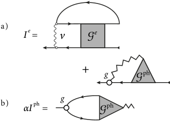
Figure 1: Diagrammatic representation of the collision integrals in terms of high order Green’s functions. Full lines are used for $G$ and zig-zag lines are used for $D$.

Equations (7) and (LABEL:eq:eomrho:b) are not closed because the collision integrals $I^{e}$ and $\mathbfit{I}^{\text{ph}}$ are proportional to the more complicated correlators $\bm{\mathcal{G}}^{e}$ and $\bm{\mathcal{G}}^{\text{ph}}$, respectively, see Fig. 1. Explicitly

$$\mathcal{G}^{e}_{imjn} =-\langle\hat{d}_{n}^{\dagger}\hat{d}_{j}^{\dagger}\hat{d}_{i}\hat{d}_{m}\rangle_{c}, \mathcal{G}^{\text{ph}}_{\mu,ij} =\langle\hat{d}_{j}^{\dagger}\hat{d}_{i}\hat{\phi}_{\mu}\rangle_{c}.$$ (8)

In paper I we have shown using the generalized Kadanoff-Baym ansatz (GKBA) [39] that they, in turn, fulfill their own equations of motions: for electrons in 2B and $T^{pp}$ approximations [40, 41]

$$i\frac{d}{dt}\bm{\mathcal{G}}^{e}(t)=-\bm{\Psi}^{e}(t)+\left[\mathbfit{h}^{e}(t)+a\bm{\rho}^{\Delta}(t)\mathbfit{v}(t)\right]\bm{\mathcal{G}}^{e}(t)\\ -\bm{\mathcal{G}}^{e}(t)\left[\mathbfit{h}^{e}(t)+a\mathbfit{v}(t)\bm{\rho}^{\Delta}(t)\right].$$ (11)

And, similarly, for phonons [34]

$$i\frac{d}{dt}\bm{\mathcal{G}}^{\text{ph}}(t) =-\bm{\Psi}^{\text{ph}}(t)+\mathbfit{h}^{\text{ph}}(t)\bm{\mathcal{G}}^{\text{ph}}(t)-\bm{\mathcal{G}}^{\text{ph}}(t)\mathbfit{h}^{e}(t),$$ (12)

We consistently use bold symbols to denote rank-2 matrices with phononic indices (viz. Eq. LABEL:eq:eomrho:b and 12) or electronic superindices (Eq. 11). The constant $a$ in Eq. (11) is equal to 0 for the second Born (2B) approximation and to 1 for the $T$-matrix approximation in the $pp$ channel ($T^{pp}$). In these equations $\mathbfit{v}$ is the Coulomb tensor, $\bm{\rho}^{\Delta}=\bm{\rho}^{>}-\bm{\rho}^{<}$, and

$$\bm{\Psi}^{e}(t) \equiv\bm{\rho}^{>}(t)\mathbfit{v}(t)\bm{\rho}^{<}(t)-\bm{\rho}^{<}(t)\mathbfit{v}(t)\bm{\rho}^{>}(t),$$ (13a)

$$\bm{\Psi}^{\text{ph}}(t) \equiv\mbox{\boldmath$\gamma$}^{>}(t)\mbox{\boldmath$g$}(t)\bm{\rho}^{<}(t)-\mbox{\boldmath$\gamma$}^{<}(t)\mbox{\boldmath$g$}(t)\bm{\rho}^{>}(t),$$ (13b)

are the driving terms. We refer to paper I for the details related to the index order of these quantities. To close the KBE one additionally needs to propagate the position and momentum expectation values $\phi_{\nu}(t)=\langle\hat{\phi}_{\nu}(t)\rangle$ because they enter $h^{e}$

$$i\frac{d}{dt}\phi_{\mu}(t)-\sum\nolimits_{\nu}h_{\mu\nu}^{\text{ph}}(t)\phi_{\nu}(t)=\sum\nolimits_{\nu ij}\alpha_{\mu\nu}g_{\nu,ij}\rho_{ji}(t).$$ (14)

Equations (12) and (11) together with EOMs for the electronic and phononic density matrices [Eqs. (7) and (LABEL:eq:eomrho:b)] and the equation of motion for $\phi(t)$ [Eq. (14)], form a closed system of ordinary differential equations (ODE).

III 1D Holstein-Hubbard model out of equilibrium

The most demanding part of the GKBA+ODE calculations is the solution of the electronic two-particle equation (11), whereby the matrix product $\mathbfit{v}\bm{\mathcal{G}}$ scales as $\mathcal{O}(N_{\text{$e$-basis}}^{6})$, with the number of electronic basis functions $N_{\text{$e$-basis}}$. The scaling can be improved relatively easy by imposing additional physically motivated restrictions on the matrix elements of $\mathbfit{v}$. This brings us to the consideration of the extended Hubbard model.

In the extended Hubbard model, which is the target of our numerical implementation, there are two classes of Coulomb integrals expressed in a site basis

$$v^{d}_{ij} =v_{ijji}, v^{x}_{ij} =v_{ijij}.$$ (15)

All other Coulomb matrix elements are set to zero. This reduces the complexity of the correlated GKBA methods to $\mathcal{O}(N_{\text{$e$-basis}}^{5})$. In our implementation we exploit this simplification whenever condition (15) is fulfilled. The implementation is otherwise completely general and can be used, for instance, to study screening at the level of the $GW$ approximation [35, 42, 43, 41].

In this work, we focus on the dynamics of electrons and phonons in the 1D one-band Holstein-Hubbard (h-h) model, where each site is coupled to a phonon,

$$\hat{H}_{\text{h-h}}=-h\sum_{\sigma=\uparrow,\downarrow}\sum_{<\bm{i},\bm{j}>}\hat{d}_{\bm{i}\sigma}^{\dagger}\hat{d}_{\bm{j}\sigma}+U\sum_{\bm{i}}\hat{n}_{\bm{i}\uparrow}\hat{n}_{\bm{i}\downarrow}\\ +\sum_{\bm{i}}\left\{\omega\hat{a}^{\dagger}_{\bm{i}}\hat{a}_{\bm{i}}+g(\hat{a}^{\dagger}_{\bm{i}}+\hat{a}_{\bm{i}})\hat{n}_{\bm{i}}\right\}.$$ (18)

Here $h$ is the matrix element of the nearest neighbor hopping ($<\bm{i},\bm{j}>$ are the neighboring sites), $U$ is the onsite Hubbard repulsion (therefore $v^{d}_{\bm{ij}}=U\delta_{\bm{ij}}$ and $v^{x}=0$ in Eq. 15), $\sigma$ is the spin projection, $\omega$ is the frequency of phonons equal at all sites, i. e. $\omega_{\bm{\mu}}=\omega$ in Eqs. (5), and $g$ is the coupling matrix element of the phonon displacement at site $\bm{i}$ to the total electron density at the same site ($\hat{n}_{\bm{i}}=\sum_{\sigma}\hat{n}_{\bm{i}\sigma}$, $\hat{n}_{\bm{i}\sigma}=\hat{d}_{\bm{i}\sigma}^{\dagger}\hat{d}_{\bm{i}\sigma}$), explicitly $g_{\mu,ij}=\sqrt{2}g\delta_{\bm{i}\bm{j}}\delta_{\bm{\mu}\bm{i}}\delta_{\xi,1}$ in Eq. (6), where the $\sqrt{2}$ prefactor is in accordance with the definition of the phononic displacement in Eq. (1). The dynamics is triggered by the creation of an electron (or a pair of them with zero total spin) at a given lattice site. The lattice is otherwise empty. Here, we denote $N=N_{\text{$e$-basis}}=N_{\text{$b$-basis}}$ — the number of single particle electronic and phononic basis functions. In what follows we measure energies in the units of $h$ and times in the units of $1/h$, therefore the system is characterized by a set of three parameters $\{U,\,\omega,\,g\}$. For the ease of reporting total energies, we eliminated the zero-point vibrational energy $\tfrac{1}{2}N\omega$ from the Hamiltonian (18) in comparison with Eq. (5).

Table 1: Largest systems and computational resources (Xeon Gold 5218 CPU @ 2.30GHz) used in this work.

System	Correlations		State	Time	CPU hours
$N$	$e$-$e$	$e$-ph	vector	$t_{\text{f}}$	$e$-$e$	$e$-ph
151	HF	Ehrenfest	23 254	40	$0.02$	$0.07$
151	HF	$GD$	7 046 264	40	$3.8$	$2.0$
151	2B	$GD$	526 954 666	40	$181.2$	$2.0$
151	$T^{pp}$	Ehrenfest	519 931 656	40	$482.8$	$0.04$
151	$T^{pp}$	$GD$	526 954 666	40	$488.0$	$2.6$

The scenario with a single electron has been studied in a number of works using different methods. Fehske et al. [44] used the Chebyshev expansion technique to solve the Schrödinger equation in a truncated bosonic basis and to study the polaronic cloud formation characterized by the diagonal $\langle\hat{n}_{\bm{i}}(\hat{a}^{\dagger}_{\bm{i}+\bm{x}}+\hat{a}_{\bm{i}+\bm{x}})\rangle$ ($\bm{x}=0$) correlator, and the phonon emission and reabsorption processes leading to the electron effective mass enhancement in a smaller system comprising only 17 sites. Interference/reflection of the electron wave-packet from the boundaries prevent clear interpretation at larger times. Similar a wave-function (WF) approach has been used by Golež et al. [26] to study the relaxation dynamics of the Holstein polaron, which they characterized by a single relaxation time $\tau$ and showed it to be proportional to $h/g^{2}$ (in the notation of Eq. 18). To identify the polaron they used a more complicated correlator $\gamma(x)=\sum_{\bm{i}}\langle\hat{n}_{\bm{i}}\hat{a}^{\dagger}_{\bm{i}+\bm{x}}\hat{a}_{\bm{i}+\bm{x}}\rangle$. Chen, Zhao and Tanimura applied the hierarchical equations of motion to exciton-phonon coupled systems and likewise found excitonic localization [16]. This is a very relevant scenario of the energy transfer in organic molecules and in photovoltaic devices. Finally, Kloss et al. [30] were able to invistigate larger 1D and 2D systems using the matrix product state (MPS) method. The objective was to study the self-localized behavior in $e$-ph systems and to demostrate the computational benefits offered by the tensor network states. Here we demonstrate that GKBA+ODE approach not only allows to study large systems of comparable spatial extent, but also to incorporate $e$-$e$ interactions without imposing any restrictions on the number of particles or the system dimensionality (see Tab. 1 for a summary of systems and computational resources). This represents two great benefits of the GF methods in contrast to other approaches: the dimension of the Hilbert space in the WF approach grows factorially with the number of particles, whereas the MPS approach is more suited for 1D systems.

Our numerical investigations are structured as follows. In the first step we establish that for the treatment of the time-evolution of a correlated spin-0 pair of electrons the $T$-matrix method in the $pp$ channel is the most appropriate. We demonstrate this by comparing with the exact solution in the absence of phonons. We will contrast very similar exact and $T^{pp}$ results with the results from time-dependent Hartree-Fock (TDHF) and from the second Born (2B) approximations. We then add $e$-ph interactions and compare the localization of the electronic wave-packets at different $e$-$e$ interaction strengths.

IV Spreading of the two-electron wave-packet on the 1D lattice

Here we consider the pure electronic case ($g=0$). The respective (Hubbard) Hamiltonian is denoted as $\hat{H}_{\text{h}}$ (cf. Eq. 18). Electronic evolution starts from the following initial condition

$$|\psi_{i}\rangle \equiv|\psi(t=0)\rangle=\hat{d}_{\bm{i}_{0}\uparrow}^{\dagger}\hat{d}_{\bm{i}_{0}\downarrow}^{\dagger}|0\rangle,$$ (26)

where $|0\rangle$ is the vacuum (empty) state, and $\bm{i}_{0}$ is the lattice site (typically in the middle of the 1D chain) where the electrons are added.

The exact two-electron singlet wave-function can be represented in a matrix form as

$$|\psi(t)\rangle =\sum_{\bm{ij}}\frac{C_{\bm{ij}}(t)}{2}\left(\hat{d}_{\bm{i}\uparrow}^{\dagger}\hat{d}_{\bm{j}\downarrow}^{\dagger}-\hat{d}_{\bm{i}\downarrow}^{\dagger}\hat{d}_{\bm{j}\uparrow}^{\dagger}\right)|0\rangle,$$ (27)

with symmetry $C_{\bm{ij}}=C_{\bm{ji}}$. It is normalized as $\langle\psi(t)|\psi(t)\rangle=\sum_{\bm{ij}}|C_{\bm{ij}}(t)|^{2}=1$ and fulfills the EOM $i\frac{d}{dt}|\psi(t)\rangle=\hat{H}_{\text{h}}|\psi(t)\rangle$

$$i\dot{C}_{\bm{ij}}(t)=-\left(C_{\bm{i}+\bm{1},\bm{j}}+C_{\bm{i}-\bm{1},\bm{j}}+C_{\bm{i},\bm{j}+\bm{1}}+C_{\bm{i},\bm{j}-\bm{1}}\right)\\ +U\delta_{\bm{ij}}C_{\bm{ij}},$$ (30)

with a boundary condition that $C_{\bm{ij}}=0$ if $\bm{i},\bm{j}=0,\,N+1$, where $N$ is the number of lattice sites.

Our main observables are the density matrix

$$\rho^{<}_{\bm{ij},\sigma}(t) \equiv\langle\psi(t)|\hat{d}_{\bm{j}\sigma}^{\dagger}\hat{d}_{\bm{i}\sigma}|\psi(t)\rangle=\sum_{\bm{n}}C^{*}_{\bm{in}}(t)C_{\bm{jn}}(t),$$ (31a)

the electronic states’ occupation numbers (independent of spin)

$$n_{\bm{i},\sigma}(t) \equiv\langle\psi(t)|\hat{n}_{\bm{i}\sigma}|\psi(t)\rangle=\sum_{\bm{n}}|C_{\bm{in}}(t)|^{2},$$ (31b)

and the doublon occupations

$$d_{\bm{i}}(t)\equiv\langle\psi(t)|(\hat{n}_{\bm{i}\uparrow}-n_{\bm{i}\uparrow})(\hat{n}_{\bm{i}\downarrow}-n_{\bm{i}\downarrow})|\psi(t)\rangle\\ =|C_{\bm{ii}}(t)|^{2}-n_{\bm{i}\uparrow}n_{\bm{i}\downarrow}.$$ (31e)

Electron dynamics described by Eq. (30) is not trivial and represent a stringent test for approximations of MBPT. Even the dynamics of a single electron on a lattice is quite different from the continous wave-packet spreading, which is well-known from quantum mechanics. The difference comes from the form of the initial state (26), which is spatially too narrow in comparison with the lattice spacing as discussed by Schönhammer [45].

The electronic group velocity $v_{e}$ is bounded:

$$v_{e} =\left.\frac{d\epsilon(k)}{dk}\right|_{k=k_{f}}\leq 2h.$$ (32)

Here $\epsilon(k)=-2h\cos(k)$ is the electron momentum dispersion relation and $k_{f}$ is a center in momentum space of the fastest moving component of the wave-packet. When there are more electrons in the system, the Hubbard interaction complicates the picture due to the appearence of the resonant doublon states [46, 29]. Since the doublon dispersion differs from the electron dispersion by a prefactor: $E(k)=-J\cos(k)$, where $J=4h^{2}/U$ (well justified for $U\gg h$) is the superexchange coupling constant [29], the doublon group velocity $v_{d}$ is in general different from the electronic one. This difference between the $v_{e}$ and $v_{d}$ can be appreciated by comparing blue and orange lines in Fig. 2.

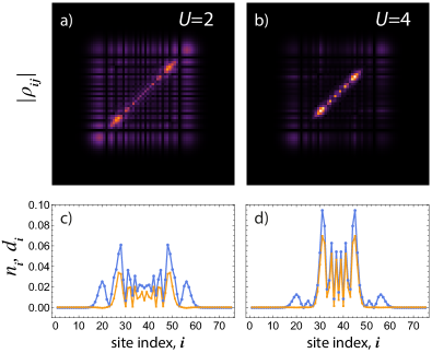
Figure 2: Electronic properties of the 1D Hubbard chain of length $N=75$ comprising two electrons from the exact solution of Eq. (30) with the initial condition $C_{ij}(0)=\delta_{ii_{0}}\delta_{ji_{0}}$ with $i_{0}=38$. Top row: snapshots at time $t=10$ of the electronic density matrix. Bottom row: electron (blue) and doublon (orange) occupation numbers computed according to Eq. (31b) and Eq. (31e), respectively.

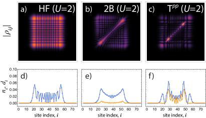
Figure 3: Moderate Hubbard repulsion $U=2$: snapshots at time $t=10$ of the electronic density matrix (top row) and the state (blue lines) and doublon (orange lines) occupations (bottom row) obtained using GKBA+ODE with different approximations.

Figure 4: Strong Hubbard repulsion $U=4$: snapshots at time $t=10$ of the electronic density matrix (top row) and the state (blue lines) and doublon (orange lines) occupations (bottom row) obtained using GKBA+ODE with different approximations.

In Figs. 3, 4, the performance of three different methods: time-dependent Hartree-Fock (HF), second Born approximation and the $T$-matrix approximation in the $pp$ channel is compared against these exact results. The initial condition for the electronic density matrix corresponding to the initial state Eq. (26) reads

$$\rho_{\bm{ij},\sigma}(t=0) =\delta_{\bm{ii}_{0}}\delta_{\bm{ji}_{0}}, \bm{\mathcal{G}}^{e}(t=0) =0,$$ (33)

meaning that the two electrons (with spin $\uparrow$ and $\downarrow$) are initially uncorrelated.

As expected, the mean-field method is completely inadequate for the 1D Hubbard model considered here: the electronic density matrix features a four-fold symmetry pertinent to noninteracting particles. A bit more accurate is the 2B method. It correctly predicts the density localization at the diagonal, however, it fails to describe the spreading of doublons: at $U=2$ they propagate with nearly the same velocity as electrons (Fig. 3). The situation seems to be different from the half-filled case, where already 2B approximation is accurate for the prediction of doublons [47]. Only $T^{pp}$ provides good agreement with the exact solution for the two-electron system considered here for intermediate ($U=2$) and large ($U=4$) Hubbard repulsion. This can be seen in the density matrix plots in Figs. 3, 4, as well as in Fig. 5, where we zoom in into the electron and doublon occupation numbers as functions of the lattice site. These two observables can be directly obtained from the GKBA+ODE approach. The first one, the electron occupation number is given by

$$n_{\bm{i},\sigma}(t) =\rho^{<}_{\bm{ii},\sigma}(t).$$ (34)

For spin-compensated systems as considered here, $\rho_{\bm{ij},\uparrow}=\rho_{\bm{ij},\downarrow}$, which allows to drop the spin index, i.e., $n_{\bm{i}}\equiv n_{\bm{i},\sigma}$.

The second observable, the number of doublons $d_{\bm{i}}(t)$ as a function of the site number $\bm{i}$, can be considered in parallel to the wave-function approach presented above. Puig von Friesen, Verdozzi and Almbladh demonstrated how this quantity can be computed in the full Kadanoff-Baym method applied to the $T$-matrix approximation [48]. In the GKBA+ODE scheme the doublon occupations are expressed in terms of the two-body correlator $\bm{\mathcal{G}}^{e}(t)$

$$d_{\bm{i}}(t) =\langle\psi(t)|\hat{n}_{\bm{i}\uparrow}\hat{n}_{\bm{i}\downarrow}|\psi(t)\rangle-n_{\bm{i}\uparrow}(t)n_{\bm{i}\downarrow}(t)=-\mathcal{G}^{e}_{\bm{iiii}}(t).$$ (35)

Notice that we are talking here about the correlated part of the doublon occupation number as defined by Eq. (31e). Not only Fig. 5 demonstrates excellent agreement between the exact and the $T^{pp}$-matrix methods, it also nicely illustrates the difference between two different group velocities $v_{e}$ and $v_{d}$.

Notice that on physical grounds we do not expect similar performance from $GW$ and $T^{ph}$ methods (they reflect correlations in particle-hole channels, which are not relevant here). Therefore, all subsequent results with phonons will be presented only for these three methods: HF, 2B and $T^{pp}$. 2B approximation is accurate only for initial instances of time. At larger times the population of doublons according to the 2B approximation diminishes, in contrast with the prediction of the $T^{pp}$ approximation, which is in good agreement with exact results (see inset of Fig. 5). Spectral properties of two-electron systems have also been studied with similar conclusions: $T^{pp}$ is very accurate, whereas 2B approximation underestimates the binding energy of a Cooper pair (see Fig. 13.5 in Ref. [49]).

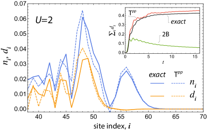
Figure 5: Comparison of the electron $n_{\bm{i}}\equiv n_{\bm{i},\sigma}$ (blue) and doublon occupations $d_{\bm{i}}$ (orange) for a Hubbard chain with $N=75$ at time $t=10$ illustrating the difference in the corresponding group velocities. Due to the inversion symmetry only a half of the system is shown. The inset depicts the total number of doublons in the system from the exact time-evolution vs. 2B and $T^{pp}$ approximations.

V Role of phonons: Ehrenfest vs. $GD$ approximation

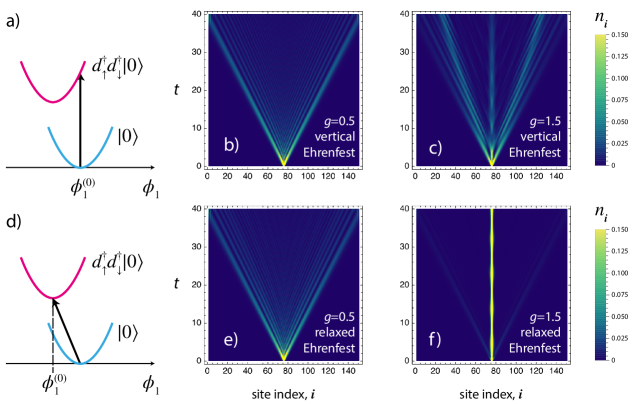
Figure 6: Evolution of the electronic density $n_{\bm{i}}\equiv n_{\bm{i},\sigma}$ for different $e$-ph interaction strengths and initial states as a function of time ($t$) and lattice site $\bm{i}$. Phonons are treated semiclassically, i. e., in the Ehrenfest approximation. Top row depicts the case of a “vertical” initial state (41) for phonons, bottom row — the “relaxed” initial state (42). In panels (a) and (d) these two scenarios are schematically depicted for the $\bm{i}_{0}$ lattice site. Panels (b) and (e) the negligible effect of the initial state for the case of weak $e$-ph interaction ($g=0.5$). Panels (c) and (f) demonstrate that for the strong $e$-ph interaction ($g=1.5$) the electronic density is localized at the central site when the dynamics is started from the relaxed phononic state. Initial electronic density matrix is the same in all cases and is given by Eq. (33).

While the Holstein model is not solvable for arbitrary parameters, there are regimes where the system behavior can be understood at least qualitatively. If the mass of a phonon is much larger than the mass of an electron, the system is in the adiabatic regime. It is characterized by the well-defined potential energy surfaces and large stiffness of the lattice and is attained for $\omega/h\ll 1$. In the opposite anti-adiabatic limit the phonons adjusts almost instantaneously to the motion of an electron. We consider here the more intriguing cross-over regime $\omega/h=1$.

The binding energy of a polaron can be estimated perturbatively [4] as

$$\varepsilon_{p} =-\frac{g^{2}}{\omega}.$$ (36)

By comparing it with the electronic band-width of $2h$ we arrive at the second important ratio:

$$\lambda =\frac{g^{2}}{2h\omega}.$$ (37)

When $\lambda\ll 1$, electrons in a small portion of the Brillouin zone around the band bottom are affected by phonons, lattice distortions spread over many lattice sites, and one classifies this quasiparticle as the “large” or “light” polaron. The polaron effective mass is enhanced as compared to the mass of an electron, however, the mass renormalization depends only on the phononic frequency, and not on the interaction strength. We will see below that this is not the case for our simulations. In the opposite limit of the so-called “small” or “heavy” polaron all electronic states are dressed by phonon [21]. A large exponential renormalization of the hopping constant is a marked physical phenomenon in this limit [49]:

$$\tilde{h} =he^{-g^{2}/\omega^{2}}.$$ (38)

Here we consider two values $e$-ph coupling $g=0.5$ and $1.5$ corresponding to $\lambda=0.125$ and $1.125$, respectively.

We start the investigation of the $e$-ph dynamics with the simplest semiclassical treatment of the optical phonons and without $e$-$e$ interactions ($U=0$). This is the scenario of Kloss et al. [30], earlier investigations are by Sayyad and Eckstein [50] (initially hot electron distribution, DMFT), Dorfner et al. [28] (diagonalization in a limited functional space). While the methods are very different, in our approach we can treat systems of comparative sizes (we use $N=151$ for all subsequent results) and even with $e$-$e$ interactions (next section). Since now the phononic subsystem is included, the initial conditions for the electrons are supplemented with the conditions for the phononic density matrix $\bm{\gamma}^{<}$, the electron-phonon two-body correlator $\bm{\mathcal{G}}^{\text{ph}}$ and the phononic coordinates $\phi$

$$\gamma^{<}_{\bm{i}\xi,\bm{j}\zeta}(t=0) =\delta_{\bm{ii}_{0}}\delta_{\bm{ji}_{0}}\gamma^{(0)}_{\xi\zeta}, \gamma^{(0)} =\frac{1}{2}\begin{pmatrix}1&-i\\ i&1\end{pmatrix};$$ (39a)

$$\bm{\mathcal{G}}^{\text{ph}}(t=0) =0;$$ (39b)

$$\phi_{\bm{i},\xi}(t=0) =\delta_{\bm{ii}_{0}}\phi^{(0)}_{\xi}.$$ (39c)

Eq. (39a) indicates that the initial phononic state is a coherent state

$$|\varphi_{i}\rangle \equiv|\varphi(t=0)\rangle=e^{\beta\hat{a}_{\bm{i}_{0}}^{\dagger}-\beta^{*}\hat{a}_{\bm{i}_{0}}}|0\rangle.$$ (40)

Eq. (39b) implies that there are no $e$-ph correlations initially. In parallel to Kloss et al. [30], two scenarios for the initial phononic displacements $\phi^{(0)}_{\xi}$ are considered. In the first one, Fig. 6(a), a vertical transition takes place from the vacuum state with zero number of electrons and phonons to a state with two electrons. In this case the phonons retain their averaged values of the displacement and momentum:

$$\bm{\phi}^{(0)} =\langle\varphi_{i}|\hat{\phi}_{\bm{i}_{0}}|\varphi_{i}\rangle=0, \beta =0.$$ (41)

In the second relaxed scenario, Fig. 6(b), it is assumed that the phonon coupled to the excitation site $\bm{i}_{0}$ is instantly displaced to a new minimum of the potential energy surface:

$$\bm{\phi}^{(0)} =\langle\varphi_{i}|\hat{\phi}_{\bm{i}_{0}}|\varphi_{i}\rangle=\begin{pmatrix}-g/\omega\\ 0\end{pmatrix}, \beta =-g/\left(\sqrt{2}\omega\right).$$ (42)

Time-evolution of the electronic occupations in the presence of classical phonons, i. e., Ehrenfest approximation ($\bm{\gamma}^{<}(t)=\bm{\gamma}^{<}(0)$, only Eq. (14) for $\phi_{\mu}$ is solved for phonons), is depicted in Fig. 6(central and right columns). For $g=0.5$ [panels (b) and (e)], the electron wave-packet spreads without any localization, and the effect of initial state on the electron dynamics is negligible. For stronger $e$-ph interaction [$g=1.5$ panels (c) and (f)] the effect of initial phononic state is strong. One observes an almost complete localization starting from the relaxed configuration, which is rather unphysical. In particular, it would be impossible to explain the localization by the phononic renormalization of the hopping parameter.

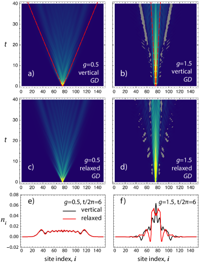
Figure 7: (a-d) Evolution of the electronic density of the $N=151$ Holstein-Hubbard chain for different $e$-ph interaction strengths and initial states. Dashed lines in panels (a) and (b) schematically depict light-cones corresponding to the renormalized group velocity $v_{e}e^{-g^{2}/\omega^{2}}$. (e-f) electronic densities at time $t/(2\pi)=6$. $e$-ph correlations are treated on the $GD$ level.

However, if we add the $e$-ph correlation effects at the $GD$ level (Fig. 7), a dramatic improvement in the spatial extent of the electron density can be seen in close agreement with the finding of Ref. [30] that “the Franck-Condon excitation is seen to retain a substantial mobility even under strong coupling”. The electron group velocity reduction is well described by Eq. (38) as indicated by red dashed lines.

We also notice that GKBA+ODE approach may sometimes lead to negative electronic densities (Fig. 4(f) and grey areas in Fig. 7) even though the total number of particles is conserved. The weight of these domains is typically very small and only causes numerical instabilities when the $e$-ph coupling constant is large. We mention in passing that negative populations have been observed also in NEGF simulations with memory truncation [51].

Next, we look at the phononic observables, starting with the site-resolved averaged values of the displacement and momentum, Fig. 8. Our main finding here is that the phase trajectories approach limiting cycles at the Ehrenfest level (in line with Ref. [52]), whereas they are not closed at the $GD$ level (this difference is more pronounced for $g=1.5$) indicating a damping of the phononic subsystem. This important physical phenomenon has also been studied in the context of polaron relaxation [26]. We will revisit this issue in the next section when discussing the total energy conservation.

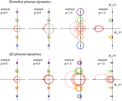
Figure 8: Phase portrait of the five central phonons of the $N=151$ Holstein-Hubbard chain. Ehrenfest (top) and $GD$ (bottom) results are compared different $e$-ph interactions and initial states.

VI Role of $e$-$e$ interactions and phonons

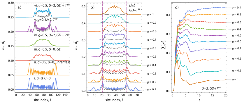
Figure 9: (a) Electron occupations (color) and doublon occupations (thin black) at time $t=20$ for all used methods and a vertical initial state. (b) Snapshots at $t=16$ of the electronic occupations (color) and doublon occupations for Holstein-Hubbard model with $N=75$ for different $e$-ph interaction strengths. (c) Time-evolution of the total number of doublons in the system for different $e$-ph interaction strengths.

In Sec. IV we have demonstrated that electron dynamics in the presence of $e$-$e$ interactions is modified by the formation and propagation of doublon excitations. Electron density matrix is fragmented into a diagonal part hosting doublons and off-diagonal part describing singly-occupied lattice sites. In Sec. V we have considered the effect of phonons on the non-interacting electrons and have shown how it reduces their group velocity leading to self-trapping. In Fig. 9(a) we summarize the results of different methods with and without $e$-$e$ and $e$-ph interactions. It can be seen that they have very different effects on the system dynamics (cf. subpanels v and iii).

It is well known that phonons hybridize with a variety of electronic excitations: plasmons [53, 54, 55], excitons [16, 56, 57], polaritons [58], collective amplitude modes in superconductors [59]. Much less is known about the coupling of doublons and phonons, being a topic of current intense investigations [60]. The effect has been studied almost exclusively in the half-filled case, where it was shown that phonons hybridize and modify the doublon dispersion relation [61], the phonon-assisted decay of excess doublons and the phonon-enhanced doublon production was predicted [36]. But what happens in the two-electron case?

In order to elucidate the simultaneous effect of $e$-$e$ and $e$-ph interactions, we fixed $U=2$ and performed a series of calculations for various electron-phonon interaction strengths, Fig. 9(b). Here we clearly see the already discussed self-trapping of electrons. It is reflected in the width reduction of the electronic distributions (depicted in color). Quite remarkably, however, the effect of the $e$-ph interaction on the distribution of doublons (thin black lines) is minimal. To facilitate the comparison, vertical dashed lines in Fig. 9(b) mark the position of the fastest doublon peaks for $g=0.1$. Increasing $e$-ph interaction from $0.1$ to $0.7$, a slight increase of the width of doublon distribution becomes evident, a part of the doublon density can be found outside the marked domain. By increasing $g$ further, the doublon distribution is squeezed again, whereby the peak position for $g=1$ coincides with the vertical line. This non-monotonous behaviour indicates that two competing physical phenomena are at play. A qualitative understanding is provided by the superexchange expression for the doublon hopping constant $J=4h^{2}/U$, which is the measure of the group velocity $v_{d}$. $e$-ph interaction modifies both parameters entering $J$. The Hubbard-$U$ constant is renormalized due to the emergence of the effective $e$-$e$ interaction mediated by phonons [2]. From general arguments, the effect is positive and nonlocal in time [62]. In the extreme antiadiabatic regime the interaction becomes instantaneous leading to an effective Hubbard model with a reduced $U$ value [63] — hence the enhancement of $v_{d}$. However, for the cross-over case $\omega=h$ considered here, the effect is small, and therefore for larger $g$ the exponential renormalization of the hopping constant according to Eq. (38) becomes the dominant mechanism. It leads to the slow-down of the doublon spreading seen for $g\geq 0.8$.

In Fig. 9(c), the total number of doublons in the system is plotted as a function of time for different $e$-ph coupling strengths. It features a rapid increase of the population at initial stage, followed by a depopulation (for $g\geq 0.3$) after which a steady value is reached in an oscillatory fashion on a much longer time scale. In line with the discussion above, the steady number of doublons is a monotonically decreasing function of $g$ confirming again the renormalization of the Hubbard-$U$ by $e$-ph interactions.

The discussion of the doublon dynamics is facilitated by the analysis of the total energy and its various contributions:

$$E(t)=E_{e,\,\text{MF}}(t)+E_{\text{ph,\,MF}}(t)+E_{\text{$e$-ph,\,MF}}(t)+E_{\text{c}}(t).$$ (43)

The mean-field energy contributions are defined as follows:

$$E_{e,\,\text{MF}}(t) =\frac{1}{2}\text{Tr}[(h(t)+h_{\text{HF}})\rho(t)],$$ (44a)

$$E_{\text{ph,\,MF}}(t) =\text{Tr}[\bm{\Omega}(t)\bm{\Gamma}(t)],$$ (44b)

$$E_{\text{$e$-ph}}(t) =\text{Tr}[h^{\text{$e$-ph}}(t)\rho(t)],$$ (44c)

with $\Gamma_{\mu\nu}(t)=\gamma_{\mu\nu}^{<}(t)+\phi_{\mu}(t)\phi_{\nu}(t)$ being the full phononic density matrix. The correlation energy $E_{\text{c}}$ is associated with $\bm{\mathcal{G}}^{e}$ and $\bm{\mathcal{G}}^{\text{ph}}$

$$E_{\text{c}} =E_{e,\,\text{c}}+E_{\text{ph,\,c}}.$$ (45)

Explicit expressions can be formulated on the Keldysh contour:

$$E_{e,\,\text{c}}(t) =-\frac{i}{2}\int_{\gamma}d\bar{t}\,\text{Tr}\Sigma^{e}(t,\bar{t})G(\bar{t},t^{+}),$$ (46a)

$$E_{\text{ph,\,c}}(t) =\frac{i}{2}\int_{\gamma}d\bar{t}\,\text{Tr}\mathbfit{\Sigma}^{\text{ph}}(t,\bar{t})\mathbfit{D}(\bar{t},t^{+}),$$ (46b)

where $\Sigma^{e}$ and $\mathbfit{\Sigma}^{\text{ph}}$ is electronic, phononic self-energy, respectively. For conserving approximations they can be written in a symmetrized form in terms of the collision integrals:

$$E_{e,\,\text{c}}(t) =-\frac{i}{4}\text{Tr}\big{[}I^{e}(t)-\left(I^{e}(t)\right)^{\dagger}\big{]},$$ (47a)

$$E_{\text{ph,\,c}}(t) =\frac{i}{4}\text{Tr}\big{[}\bm{\alpha}\mathbfit{I}^{\text{ph}}(t)-\left(\bm{\alpha}\mathbfit{I}^{\text{ph}}(t)\right)^{\dagger}\big{]}.$$ (47b)

The two contributions are equal in the absence of $e$-$e$ interactions as has been shown in our earlier work [34]. Notice that $E_{e,\,\text{c}}$ contains a phononic part (equal to $E_{\text{ph\,c}}$) and a pure $e$-$e$ correlation energy. In Figs. 10,11, the time-evolution of the total energy ingredients is presented for two values of $e$-ph coupling strength, $g=0.5$ and $g=1.5$ and two values of $e$-$e$ coupling, $U=0$ and $U=2$. In all cases the total energy is conserved up to numerical accuracy despite the fact that correlated contributions are an order of magnitude smaller. Theories with frozen phonons obviously do not fulfill this property.

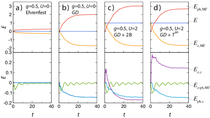
Figure 10: Time-dependent energies for the $g=0.5$ cases with vertical initial state.

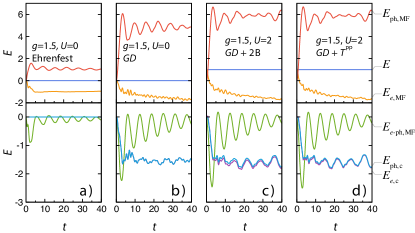
Figure 11: Time-dependent energies for the $g=1.5$ cases with vertical initial state.

The initial stage of the doublon dynamics is driven by a pure electronic mechanism. This can be concluded by comparing a very quick increase of the electronic correlational energy $E_{e,\,\text{c}}$ (proportional to the number of doublons) and a slow variation of the mean-field phononic energy $E_{\text{ph,\,MF}}(t)$ (proportional to the number of phonons) in Figs. 10 ($GD$+$T^{pp}$ results). The latter grows in time at the expense of the electron kinetic energy $E_{e,\,\text{MF}}$ [51]. In panels (a) to (b) in Figs. 10 and 11 the kinetic energy exchange between the electronic and phononic subsystems is severely underestimated. This is a shortcoming of the Ehrenfest approximation and it is cured in $GD$. Notice that the efficiency of the kinetic energy exchange increases with increasing $g$ and remains unchanged even in the presence of $e$-$e$ interaction.

By inspecting the behavior of the pure electronic correlation energy $E_{\text{$e$-$e$, c}}=E_{e,\,\text{c}}-E_{\text{ph,\,c}}$ in the asymptotic regime we conclude that for larger times the doublon-phonon scattering becomes less efficient; the energy of doublons is insufficient to excite phonon quanta — the so-called phononic bottleneck effect. In 2B pure electronic correlations given by $E_{\text{$e$-$e$, c}}$ is negative (difference between magenta and cyan lines), meaning that the density of doublons goes negative, see also panel (iv) in Fig. 9(a). This shortcoming of the 2B is cured by the $T^{pp}$ approximation.

Finally we characterize the spreading of the polaronic quasiparticle. Its spatial extension can be quantified by plotting the correlators

$$\delta_{\bm{i},\xi}(t) =\left\langle\hat{n}_{\bm{i}_{0}}(t)\hat{\phi}_{\bm{i}_{0}+\bm{i},\xi}(t)\right\rangle=\mathcal{G}^{\text{ph}}_{\bm{i}_{0}+\bm{i},\xi;\bm{i}_{0}\bm{i}_{0}}(t),$$ (48)

where $\bm{i}_{0}$ is the initial excitation site. It represents a conditional probability of a phonon at site $\bm{i}_{0}+\bm{i}$ having the mean displacement $\phi$ when an electron is at site $\bm{i}_{0}$. Therefore, it can be used as a tool to distinguish the coherent phononic cloud propagating together with the electron from uncorrelated phononic background [44]. As we already discussed above, our system in the presence of strong $e$-$ph$ interaction, behaves in many ways similar to the case with reduced $e$-$e$ coupling. This can be seen in the dynamics of doublons in Fig. 9(b), and in similarities between panels (b) and (d) in Fig. 11. Therefore, Fig. 12(c) depicts the classical picture of polaron spreading. Going to smaller values of $e$-$ph$ coupling as in Fig. 12(a, b), the effect of $U$ becomes dominant, it reduces the spectral strength and spatial extent of a polaron, representing a marked feature of electronic correlations.

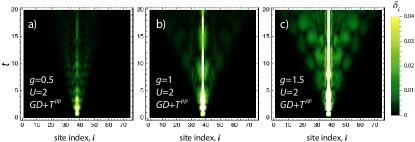
Figure 12: The $e$-ph correlator $\delta_{\bm{i}}=\sqrt{\delta_{\bm{i},1}^{2}+\delta_{\bm{i},2}^{2}}$ as a function of time for three different $e$-ph coupling constants and vertical initial state.

VII Summary

In this work, we applied a nonequilibrium Green’s function formalism (paper I) to investigate coupled electron-phonon dynamics in 1D Hubbard-Holstein model. While theories separately describing $e$-$e$ correlations or $e$-ph correlations in model systems are known, this contribution is devoted to the systems where both ingredients are important. We restrict to the $\Phi$-derivable and, therefore, conserving approximations, and consider a class of theories with an additive Baym functional consisting of the electronic and phononic parts. This leads to intertwined electronic and phononic self-energies, whereas the electronic and phononic response functions are treated independently. This approach captures with elegance the feedback in time-domain of phonons on the electronic properties and the modification of phononic properties caused by the dynamics of electrons. The method scales linearly with the physical propagation time thanks to the use of GKBA in the ODE formulation. This allows one to perform simulations for unprecedentedly large systems such as 1D chains described by the extended Holstein-Hubbard model. The model is a prototype for typical photovoltaic systems and possesses two remarkable quasiparticle states — polarons and doublons. The interplay between them leads to intricate physical phenomenon of the doublon localization that we discuss at length here. We emphasize that the phenomenon is manifested at moderate $e$-$e$ and $e$-ph interaction strengths and therefore is well suited for methods based on many-body perturbation theory. Besides the obvious observables such as electronic occupation numbers and density matrices, phase-space dynamics of individual phonons, we consider more complicated $e$-ph correlators and ingredients of the total energy.