Time-linear scaling NEGF methods for real-time simulations of interacting electrons and bosons. I. Formalism

Abstract

Simulations of interacting electrons and bosons out of equilibrium, starting from first principles and aiming at realistic multiscale scenarios, is a grand theoretical challenge. Here, using the formalism of nonequilibrium Green’s functions and relying in a crucial way on the recently discovered time-linear formulation of the Kadanoff-Baym equations, we present a versatile toolbox for the simulation of correlated electron-boson dynamics. A large class of methods are available, from the Ehrenfest to the dressed $GD$ for the treatment of electron-boson interactions in combination with perturbative, i.e., Hartree-Fock and second-Born, or nonperturbative, i.e., $GW$ and $T$-matrices either without or with exchange effects, for the treatment of the Coulomb interaction. In all cases the numerical scaling is linear in time and the equations of motion satisfy all fundamental conservation laws.

I Introduction

The electron dynamics in correlated materials is typically accompanied by the interaction with bosonic particles and quasiparticles, such as phonons, plasmons, charge density waves, photons, etc.. From the theoretical point of view the vastly different energy (or time) scales [1, 2, 3, 4, 5, 6] and the quantum nature of the involved bosonic particles [7, 8, 9, 10, 11] pose considerable challenges. A scalable quantum method to model excitation and relaxation phenomena in correlated many-body systems, reliable beyond the perturbative regime, is crucial to simulate and interpret experimental results and to design new materials. This latter aspect is especially important in view of recent progresses in light-enhanced phonon-induced superconductivity [12, 13, 14, 15], manipulation of thermoelectric properties with cavity photons [16, 17], photonics in nanojunctions [18], exciton-phonon dynamics [19, 20, 21] and light-driven chemistry [22, 23] to mention a few.

The many-body diagrammatic theory represents a systematic way to deal with interactions between electrons and bosonic particles. In order to get access to the dynamical properties of the system, the equations of motion (EOM) for the two-times electron and boson Green’s functions, hereafter referred to as the nonequilibrium Green’s function (NEGF) theory [24, 25, 26, 27], must be propagated. The EOMs in this case are known as the Kadanoff-Baym equations (KBE) [28]. The time non-locality of the scattering term represents the major difficulty for the full two-times propagation as it makes the scaling at least cubic ($t_{\text{f}}^{3}$) with the physical propagation time $t_{\text{f}}$ [29, 30, 31, 32, 33, 34, 35, 36]. This hinders the possibility of resolving small energy scales as those associated to phonons. In the purely electronic case (no bosons) the generalized Kadanoff-Baym ansatz (GKBA) [37] mitigates the problem of the cubic scaling allowing one to limit the propagation to the time-diagonal, that is, to work with density matrices rather than with two-times Green’s functions. One can work either with the integro-differential formulation, which has a quadratic ($t_{\text{f}}^{2}$) scaling in time  [38, 39, 40, 41, 42, 43, 44], or with a coupled system of first-order ordinary differential equations (ODE) thus achieving a linear ($t_{\text{f}}$) time scaling [45, 46]. The linear-time formulation has been already implemented to study the photoinduced dynamics of organic molecules [47], carrier and exciton dynamics in 2D materials [48] and the doublon production in correlated graphene clusters [49].

In our recent Letter [11] we extended the GKBA to quantized bosonic particles and formulated a first-order ODE, hence time-linear, scheme to treat systems with an electron-boson ($e$-$b$) interaction. We also stated that it is possible to include the electron-electron ($e$-$e$) interactions on equal footing. The goal of this work is to give an explicit demonstration of our statement. We will further combine the GKBA+ODE formulation with the Baym and Kadanoff theories [50, 51, 26] to generate EOM that satisfy all fundamental conservation laws. This means that the feedback of the electrons on the bosonic subsystem is consistently taken into account. Several nonperturbative methods are generated in this way, e.g., $GW$ and $T$-matrices either without or with exchange [47] for the $e$-$e$ interaction and Ehrenfest or dressed second-order ($GD$) for the $e$-$b$ interaction. The whole set of methods provides an ideal toolbox: depending on the system and the external driving one can choose the most appropriate tool to simulate the dynamics.

The paper is organized as follows. In Section II we introduce the most general system Hamiltonian and review basic notions of the NEGF formalism. We then discuss diagrammatic approximations and connections between self-energies and high order Green’s functions through the $\Phi$ functional of Baym. In Section  III we present the GKBA for electrons and bosons and show how to close the EOM for the electronic and bosonic density matrices in two different ways, using either the self-energies or the high-order Green’s functions. We subsequently derive the GKBA+ODE formulation and discuss in detail the diagrammatic content of the self-energy for all considered approximations. Conclusions and outlook are drawn in Section IV.

II Electron-boson NEGF equations for correlated systems

We consider a general electron-boson system possibly driven by external time-dependent fields and hence described by the Hamiltonian

$$\hat{H}(t)=\hat{H}_{\text{el}}(t)+\hat{H}_{\text{bos}}(t)+\hat{H}_{\text{el-bos}}(t).$$ (1)

The electronic Hamiltonian

$$\hat{H}_{\text{el}}(t) =\sum_{ij}h_{ij}(t)\hat{d}_{i}^{\dagger}\hat{d}_{j}+\frac{1}{2}\sum_{ijmn}v_{ijmn}(t)\hat{d}_{i}^{\dagger}\hat{d}_{j}^{\dagger}\hat{d}_{m}\hat{d}_{n},$$ (2)

comprises a one-body term ($h^{\dagger}=h$) accounting for the kinetic energy as well as the interaction with nuclei and possible external fields and a two-body term accounting for the Coulomb interaction between the electrons. The time-dependence of the Coulomb matrix elements $v_{ijmn}(t)$ could be due to the adiabatic switching protocol adopted to generate a correlated initial state. Henceforth we use latin letters to denote one-electron states; thus $i$ is a composite index standing for an orbital degree of freedom and a spin projection.

The annihilation and creation operators for a bosonic mode $\mu$, i.e., $\hat{a}_{\mbox{\scalebox{0.7}{$\scriptscriptstyle\mbox{\boldmath$\mu$}$}}}$ and $\hat{a}^{{\dagger}}_{\mbox{\scalebox{0.7}{$\scriptscriptstyle\mbox{\boldmath$\mu$}$}}}$, are arranged into a vector $(\hat{x}_{\mbox{\scalebox{0.7}{$\scriptscriptstyle\mbox{\boldmath$\mu$}$}}},\hat{p}_{\mbox{\scalebox{0.7}{$\scriptscriptstyle\mbox{\boldmath$\mu$}$}}})$ where $\hat{x}_{\mbox{\scalebox{0.7}{$\scriptscriptstyle\mbox{\boldmath$\mu$}$}}}=(\hat{a}^{{\dagger}}_{\mbox{\scalebox{0.7}{$\scriptscriptstyle\mbox{\boldmath$\mu$}$}}}+\hat{a}_{\mbox{\scalebox{0.7}{$\scriptscriptstyle\mbox{\boldmath$\mu$}$}}})/\sqrt{2}$ are the position operators and $\hat{p}_{\mbox{\scalebox{0.7}{$\scriptscriptstyle\mbox{\boldmath$\mu$}$}}}=i(\hat{a}^{{\dagger}}_{\mbox{\scalebox{0.7}{$\scriptscriptstyle\mbox{\boldmath$\mu$}$}}}-\hat{a}_{\mbox{\scalebox{0.7}{$\scriptscriptstyle\mbox{\boldmath$\mu$}$}}})/\sqrt{2}$ are the momentum operators. The greek index $\mu=(\mbox{\boldmath$\mu$},\xi)$ is then used to specify the bosonic mode and the component of the vector: $\hat{\phi}_{\mu}=\hat{x}_{\mbox{\scalebox{0.7}{$\scriptscriptstyle\mbox{\boldmath$\mu$}$}}}$ for $\xi=1$ and $\hat{\phi}_{\mu}=\hat{p}_{\mbox{\scalebox{0.7}{$\scriptscriptstyle\mbox{\boldmath$\mu$}$}}}$ for $\xi=2$. We write the bosonic Hamiltonian as

$$\hat{H}_{\text{bos}}(t)=\sum_{\mu\nu}\Omega_{\mu\nu}(t)\hat{\phi}_{\mu}\hat{\phi}_{\nu},$$ (3)

where $\Omega^{\dagger}=\Omega$ may depend on time, e.g., phonon drivings. The typical Hamiltonian for free bosons, i.e., $\hat{H}_{\text{bos}}(t)=\sum_{\mbox{\scalebox{0.7}{$\scriptscriptstyle\mbox{\boldmath$\mu$}$}}}\omega_{\mbox{\scalebox{0.7}{$\scriptscriptstyle\mbox{\boldmath$\mu$}$}}}\left(\hat{a}^{{\dagger}}_{\mbox{\scalebox{0.7}{$\scriptscriptstyle\mbox{\boldmath$\mu$}$}}}\hat{a}_{\mbox{\scalebox{0.7}{$\scriptscriptstyle\mbox{\boldmath$\mu$}$}}}+\tfrac{1}{2}\right)$, follows from Eq. (3) when setting

$$\Omega_{\mu\mu^{\prime}}=\frac{1}{2}\delta_{\mbox{\scalebox{0.7}{$\scriptscriptstyle\mbox{\boldmath$\mu$}$}}\mbox{\scalebox{0.7}{$\scriptscriptstyle\mbox{\boldmath$\mu$}$}}^{\prime}}\omega_{\mbox{\scalebox{0.7}{$\scriptscriptstyle\mbox{\boldmath$\mu$}$}}}\delta_{\xi\xi^{\prime}},$$ (4)

see also paper II. If the bosons are photons then $\mbox{\boldmath$\mu$}={\bf p}$ is the momentum and $\omega_{{\bf p}}=c|{\bf p}|$, with $c$ the speed of light.

The electronic and bosonic subsystems interact through

$$\hat{H}_{\text{el-bos}}(t) =\sum_{\mu,ij}g_{\mu,ij}(t)\hat{d}_{i}^{\dagger}\hat{d}_{j}\hat{\phi}_{\mu};$$ (5)

therefore electrons can be coupled to both the mode coordinates and momenta. Similarly to the Coulomb matrix elements $v$ we allow $g$ to depend on time for possible adiabatic switchings.

Without any loss of generality we work with an orthonormal basis for one-electron states and one-boson states. Then the creation and annihilation operators fulfill the standard anticommutation rules for electrons

$$\Big{\{}\hat{d}_{i},\hat{d}^{\dagger}_{j}\Big{\}} =\delta_{ij}, \Big{\{}\hat{d}^{\dagger}_{i},\hat{d}^{\dagger}_{j}\Big{\}} =\Big{\{}\hat{d}_{i},\hat{d}_{j}\Big{\}}=0,$$ (6)

and commutation rules for bosons

$$\left[\hat{\phi}_{\mu},\hat{\phi}_{\nu}\right]=\alpha_{\mu\nu},\quad\quad\alpha_{\mu\mu^{\prime}}=-\delta_{\mbox{\scalebox{0.7}{$\scriptscriptstyle\mbox{\boldmath$\mu$}$}}\mbox{\scalebox{0.7}{$\scriptscriptstyle\mbox{\boldmath$\mu$}$}}^{\prime}}\begin{pmatrix}0&-i\\ i&0\end{pmatrix}_{\xi\xi^{\prime}}.$$ (7)

II.1 NEGF formalism

In the NEGF formalism the fundamental unknowns are the electronic lesser/greater single-particle Green’s functions

$$G^{<}_{ij}(t,t^{\prime}) =i\langle\hat{d}_{j}^{\dagger}(t^{\prime})\hat{d}_{i}(t)\rangle, G^{>}_{ij}(t,t^{\prime}) =-i\langle\hat{d}_{i}(t)\hat{d}_{j}^{\dagger}(t^{\prime})\rangle,$$ (8)

and their bosonic counterparts

$$D^{<}_{\mu\nu}(t,t^{\prime}) =D^{>}_{\nu\mu}(t^{\prime},t)=-i\langle\Delta\hat{\phi}_{\nu}(t^{\prime})\Delta\hat{\phi}_{\mu}(t)\rangle.$$ (9)

In Eq. (9) we have introduced the fluctuation operators

$$\Delta\hat{\phi}_{\nu}(t) \equiv\hat{\phi}_{\nu}(t)-\langle\hat{\phi}_{\nu}(t)\rangle,$$ (10)

where the expectation value of the bosonic field operator $\phi_{\nu}(t)\equiv\langle\hat{\phi}_{\nu}(t)\rangle$ (in contrast to the electronic case) is in general nonzero. In Eqs. (8, 9, 10) the operators are in the Heisenberg picture and hence they depend on time.

The correlators $G^{\lessgtr}$ and $D^{\lessgtr}$ satisfy the integro-differential Kadanoff-Baym equations (KBE) of motion. For the electronic part they read (in matrix form):

$$\left[i\partial_{t}-h^{e}(t)\right]G^{\lessgtr}(t,t^{\prime})=\left[\Sigma^{e,\lessgtr}\cdot G^{A}+\Sigma^{e,R}\cdot G^{\lessgtr}\right]\!(t,t^{\prime}),$$ (11)

where $\left[\mathfrak{a}\cdot\mathfrak{b}\right](t,t^{\prime})\equiv\int d\bar{t}\,\mathfrak{a}(t,\bar{t})\mathfrak{b}(\bar{t},t^{\prime})$ is a real-time convolution and the superscripts “$R$” and “$A$” denote the retarded and advanced components. The quantity $\Sigma^{e}$ is the correlation part of the electronic self-energy; it is a functional of $G$ and $D$ through many-body diagrammatic treatments. The time-local mean-field part is incorporated in the effective electronic Hamiltonian $h^{e}(t)$

$$h^{e}_{ij}(t) =h_{ij}(t)+V^{{\rm HF}}_{ij}(t)+\sum_{\mu}g_{\mu,ij}(t)\phi_{\mu}(t),$$ (12)

where $V^{{\rm HF}}_{ij}=\sum_{mn}[v_{imnj}(t)-v_{imjn}(t)]\rho^{<}_{nm}(t)$ is the Hartree-Fock (HF) potential written in terms of the the electronic density matrix $\rho^{<}(t)$:

$$\rho_{ij}^{\lessgtr}(t) \equiv-iG^{\lessgtr}_{ij}(t,t), [\rho^{>}_{ij}\equiv\rho^{<}_{ij}-\delta_{ij}].$$ (13)

Analogously, for the bosonic propagators we have (in matrix form) [27]

$$\left[i\partial_{t}-\mathbfit{h}^{b}(t)\right]\mathbfit{D}^{\lessgtr}(t,t^{\prime})=\mbox{\boldmath$\alpha$}\!\left[\mathbfit{\Sigma}^{b,\lessgtr}\cdot\mathbfit{D}^{A}+\mathbfit{\Sigma}^{b,R}\cdot\mathbfit{D}^{\lessgtr}\right]\!(t,t^{\prime})$$

where $\mathbfit{\Sigma}^{b}$ is the bosonic self-energy and

$$\mathbfit{h}^{b}\equiv\mbox{\boldmath$\alpha$}(\bm{\Omega}+\bm{\Omega}^{T})$$ (14)

is the effective bosonic Hamiltonian. Like $\Sigma^{e}$ also $\mathbfit{\Sigma}^{b}$ is a functional of $G$ and $D$. To distinguish matrices in the one-electron space from matrices in the one-boson space we use boldface for the latters. If $\hat{H}_{\rm bos}$ is a sum of harmonic oscillators then $\bm{\Omega}+\bm{\Omega}^{T}$ is proportional to the identity matrix in $\xi$-space, see Eq. (4), and hence $\mbox{\boldmath$\alpha$}(\bm{\Omega}+\bm{\Omega}^{T})=(\bm{\Omega}+\bm{\Omega}^{T})\mbox{\boldmath$\alpha$}$. For simplicity we here specialize the discussion to this case.

To close the KBE one additionally needs to propagate the position and momentum expectation values appearing in Eq. (12):

$$\sum\nolimits_{\nu}\left[i\delta_{\mu\nu}\partial_{t}-h^{b}_{\mu\nu}(t)\right]\phi_{\nu}(t)=\sum\nolimits_{ij}\bar{g}_{\mu,ij}\rho_{ji}(t),$$ (15)

where we have introduced

$$\bar{g}_{\mu.ij}\equiv\sum_{\nu}\alpha_{\mu\nu}g_{\nu,ij}.$$ (16)

The KBE can also be used to generate the EOM for the electronic and bosonic density matrices. By subtracting Eq. (11) to its adjoint and taking the equal times limit ($t=t^{\prime}$) we obtain

$$\frac{d}{dt}\rho^{<}(t) =-i\big{[}h^{e}(t),\rho^{<}(t)\big{]}-\left(I^{e}(t)+I^{e\,\dagger}(t)\right),$$ (17)

where $I^{e}(t)$ is the right hand side of Eq. (11) calculated in $t=t^{\prime}$. Analogously, the subtraction of Eq. (II.1) to its adjoint and the subsequent evaluation in $t=t^{\prime}$ yields for the bosonic density matrix

$$\gamma_{\mu\nu}^{\lessgtr}(t) \equiv iD^{\lessgtr}_{\mu\nu}(t,t), [\gamma^{>}_{\mu\nu}\equiv\gamma^{<}_{\mu\nu}+\alpha_{\mu\nu}=\gamma^{<\,\ast}_{\mu\nu}]$$ (18)

the following equation of motion

$$\frac{d}{dt}\mbox{\boldmath$\gamma$}^{<}(t) =-i\big{[}\mathbfit{h}^{b}(t),\mbox{\boldmath$\gamma$}^{<}(t)\big{]}+\left(\mathbfit{I}^{b}(t)+\mathbfit{I}^{b\dagger}(t)\right),$$ (19)

where $\mathbfit{I}^{b}(t)$ is the right hand side of Eq. (II.1) for $t=t^{\prime}$. Equations (17) and (19) are not closed because the collision integrals $I^{e}$ and $\mathbfit{I}^{b}$ are still functionals of the two-times Green’s functions via the respective self-energies, $\Sigma^{e}=\Sigma^{e}[G,D;v,g]$ and $\mathbfit{\Sigma}^{b}=\mathbfit{\Sigma}^{b}[G,D;v,g]$. In Section III we shall illustrate how to close the EOM (17) and (19) through the GKBA for electrons and bosons. Preliminarly we need to develop further the NEGF theory and discuss diagrammatic approximations.

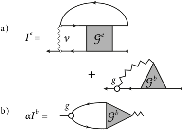
Figure 1: Diagrammatic representation of the collision integrals in terms of high order Green’s functions. Full lines are used for $G$, zig-zag lines are used for $D$, wavy lines are used for $v$ and empty circles are used for $g$.

We split the electronic self-energy into a purely electronic part $\Sigma^{ee}[G,v]\equiv\Sigma^{e}[G,D;v,g]_{g=0}$ and a rest, i.e.,

$$\Sigma^{e}=\Sigma^{ee}+\Sigma^{eb}.$$ (20)

The electronic collision integral is then the sum of two terms, one containing $\Sigma^{ee}$ and the other containing $\Sigma^{eb}$:

$$I^{e}=I^{ee}+I^{eb}.$$ (21)

From the first equation of the Martin-Schwinger hierarchy for the electronic and bosonic Green’s functions one can show that the three collision integrals $I^{ee}$, $I^{eb}$ and $\mathbfit{I}^{b}$ can also be written in terms of two high-order Green’s functions [27]:

$$\mathcal{G}^{e}_{imjn}(t) =-\langle\hat{d}^{{\dagger}}_{n}(t)\hat{d}^{{\dagger}}_{j}(t)\hat{d}_{i}(t)\hat{d}_{m}(t)\rangle_{c},$$ (22)

$$\mathcal{G}^{b}_{\mu,ij}(t) =\langle\hat{d}^{{\dagger}}_{j}(t)\hat{d}_{i}(t)\hat{\phi}_{\mu}(t)\rangle_{c}.$$ (23)

The subscript “$c$” in the averages signifies that only the correlated part must be retained. Like the self-energies also the high-order Green’s functions are functionals of $G$, $D$, $v$ and $g$. Pulling out from $\mathcal{G}^{e}$ the electronic part $\mathcal{G}^{ee}\equiv\mathcal{G}^{e}|_{g=0}$, hence

$$\mathcal{G}^{e}=\mathcal{G}^{ee}+\mathcal{G}^{eb},$$ (24)

one finds

$$I^{ee}_{lj} =-i\sum_{imn}v_{lnmi}(t)\mathcal{G}^{ee}_{imjn}(t),$$ (25a)

$$I^{eb}_{lj} =+i\sum_{\mu,i}g_{\mu,li}(t)\mathcal{G}^{b}_{\mu,ij}(t)-i\sum_{imn}v_{lnmi}(t)\mathcal{G}^{eb}_{imjn}(t),$$ (25b)

$$I^{b}_{\mu\nu} =-i\sum_{mn}\bar{g}_{\mu,mn}(t)\mathcal{G}^{b}_{\nu,nm}(t).$$ (25c)

Equations (25) establish the relation between the pair $\Sigma^{e}$ and $\mathbfit{\Sigma}^{b}$ and the pair $\mathcal{G}^{e}$ and $\mathcal{G}^{b}$; the diagrammatic content of this relation is illustrated in Fig. 1. Notice that the diagrams for $\Sigma^{eb}(t,t^{\prime})$ have either an $e$-$b$ vertex $g(t)$ or an $e$-$e$ vertex $v(t)$ at time $t$. The former provide the diagrammatic content of $\mathcal{G}^{b}$ while the latter provide the diagrammatic content of $\mathcal{G}^{eb}$, see again Eq. (25b).

It is critical to point out that for arbitrary approximations to $\Sigma^{eb}$ and $\mathbfit{\Sigma}^{b}$ the mixed Green’s function $\mathcal{G}^{b}$ entering $I^{eb}$ and $I^{b}$ need not be equal. We therefore consider only $\Phi$-derivable approximations [51, 26, 27, 11] for these quantities. The Baym functional $\Phi$ is expressed in terms of connected vacuum diagrams with $e$-$b$ and $e$-$e$ vertices. Let $\Phi_{c}[G,D;v,g]$ be the correlated part of the full Baym functional; $\Phi_{c}$ is obtained by discarding the HF and Ehrenfest vacuum diagrams, leading to the HF potential and classical nuclear potential appearing in Eq. (12). We define $\Phi^{ee}$ as the purely electronic part of $\Phi_{c}$, hence $\Phi^{ee}[G,v]=\Phi_{c}|_{g=0}$, and write

$$\Phi_{c}[G,D;v,g]=\Phi^{ee}[G,v]+\tilde{\Phi}[G,D;v,g].$$ (26)

The $\Phi$-derivable self-energies are then given by (times $t$ and $t^{\prime}$ on the Keldysh contour)

$$\Sigma^{eb}_{ij}(t,t^{\prime}) =\frac{\delta\tilde{\Phi}}{\delta G_{ji}(t,t^{\prime})},$$ (27a)

$$\Sigma^{b}_{\mu\nu}(t,t^{\prime}) =-\frac{\delta\tilde{\Phi}}{\delta D_{\nu\mu}(t,t^{\prime})}-\frac{\delta\tilde{\Phi}}{\delta D_{\mu\nu}(t^{\prime},t)}.$$ (27b)

The $\Phi$-derivability guarantees that the same high-order Green’s function $\mathcal{G}^{b}$ enters $I^{eb}$ and $I^{b}$. Alternatively, the functional dependence of $\mathcal{G}^{b}$ on $G$ and $D$ can be directly deduced from the functional derivative of $\tilde{\Phi}$ with respect to the $e$-$b$ coupling:

$$\mathcal{G}^{b}_{\mu,ij}(t) =\frac{1}{i}\,\frac{\delta\tilde{\Phi}[G,D;v,g]}{\delta g_{\mu,ji}(t)}.$$ (28)

We emphasize that the $\Phi$-derivability of $\Sigma^{eb}$ and $\mathbfit{\Sigma}^{b}$ guarantees the fulfillment of all fundamental conservation laws [52] provided that also $I^{ee}$ is calculated in a conserving manner. A sufficient condition for having a conserving $I^{ee}$ is to consider only $\Phi$-derivable electronic self-energies $\Sigma^{ee}_{ij}(t,t^{\prime})=\delta\Phi^{ee}/\delta G_{ji}(t^{\prime},t)$. This condition, however, is not necessary. We use the less stringent requirement of the symmetry of the two-particle Green’s function (2-GF) [50]

$$\mathcal{G}^{ee}_{imjn}(t,t^{\prime})\equiv-\langle\hat{d}^{{\dagger}}_{n}(t)\hat{d}^{{\dagger}}_{j}(t^{\prime})\hat{d}_{i}(t^{\prime})\hat{d}_{m}(t)\rangle_{c}|_{g=0}=\mathcal{G}^{ee}_{minj}(t^{\prime},t).$$ (29)

This two-time function coincides with $\mathcal{G}^{ee}(t)$ in Eq. (24) along the time diagonal, i.e., $\mathcal{G}^{ee}(t,t)=\mathcal{G}^{ee}(t)$.

II.2 Approximations for correlated electron-boson dynamics

In several physical situations, e.g., phonon-induced carrier relaxation, Raman spectroscopy, transport through molecular junctions, etc., $\tilde{\Phi}$ is approximated as

$$\tilde{\Phi}=\raisebox{-6.0pt}{\includegraphics{Fig2}}\;\;,$$ (30)

where the $e$-$b$ vertices are either bare [53] (photon fields) or statically screened [2] (phonon fields). This is the diagrammatic approximation that we too examine in the present work. In most practical implementations the boson propagator $D$ in $\tilde{\Phi}$ is frozen at its equilibrium and noninteracting value. We go beyond this approximation and consider $\tilde{\Phi}$ as a functional of the fully dressed electronic and bosonic Green’s functions. Energy can then be transferred from the bosonic subsystem to the electronic subsystem and viceversa while the total energy is conserved. The explicit mathematical expression of $\tilde{\Phi}$ is (time integrals are over the Keldysh contour)

$$\tilde{\Phi}=\frac{i}{2}\sum_{\begin{subarray}{c}\mu\nu\\ ijsq\end{subarray}}\int\!\!dtdt^{\prime}g_{\mu,ji}(t)D_{\mu\nu}(t,t^{\prime})g_{\nu,sq}(t^{\prime})G_{is}(t,t^{\prime})G_{qj}(t^{\prime},t).$$ (31)

Through functional derivatives with respect to $G$ and $\mathbfit{D}$, see Eqs. (27), the chosen $\tilde{\Phi}$ leads to the dressed second-order self-energy ($GD$) for the electrons [54] and to the bubble self-energy for the bosons [11], see Section III.3 for more details. These self-energies give the same mixed Green’s function $\mathcal{G}^{b}$ from Eqs. (25b) and (25c) since they are derived from the same $\tilde{\Phi}$ functional.

We have seen that $\mathcal{G}^{b}$ can also be calculated from Eq. (28). Taking into account that $\Phi^{ee}$ is independent of the $e$-$b$ coupling we get

$$\mathcal{G}^{b}_{\mu,ij}(t)=\sum_{\nu,sq}\int^{t}\!\!dt^{\prime}\Big{\{}D^{>}_{\mu\nu}(t,t^{\prime})g_{\nu,sq}(t^{\prime})G^{>}_{is}(t,t^{\prime})G^{<}_{qj}(t^{\prime},t)$$

$$-(>\leftrightarrow<)\Big{\}}.$$ (32)

To highlight the mathematical structure in the right hand side we find useful to introduce a composite index for pairs of electron indices. Without any risk of ambiguity we use greek letters also for such composite index:

$$g_{\mu,ij} =g_{\mu,\begin{subarray}{c}j\\ i\end{subarray}}=g_{\mu\nu}, \mathcal{G}^{b}_{\mu,ij} \rightarrow\mathcal{G}^{b}_{\mu,\begin{subarray}{c}j\\ i\end{subarray}}=\mathcal{G}^{b}_{\mu\nu}, \nu=\begin{pmatrix}j\\ i\end{pmatrix}.$$ (33)

This mathematical notation expresses the physical notion that we need two fermions to make a boson. We can then rewrite Eq. (II.2) in a compact matrix form as

$$\bm{\mathcal{G}}^{b}(t) =i\int^{t}\!\!dt^{\prime}\Big{\{}\mathbfit{D}^{>}(t,t^{\prime})\mbox{\boldmath$g$}(t^{\prime})\bm{\mathit{\chi}}^{0,<}(t^{\prime},t)-(>\leftrightarrow<)\Big{\}},$$ (34)

where, consistently with our notation, the matrices with greek indices are represented by boldface letters. In Eq. (34) we have defined the noninteracting response function

$$\chi^{0,\lessgtr}_{\mu\nu}(t^{\prime},t)=\chi^{0,\lessgtr}_{\begin{subarray}{c}qj\\ si\end{subarray}}(t^{\prime},t)\equiv-iG^{\lessgtr}_{qj}(t^{\prime},t)G^{\gtrless}_{is}(t,t^{\prime}).$$ (35)

The diagrammatic representation of Eq. (34) is given in Fig. 2(a).

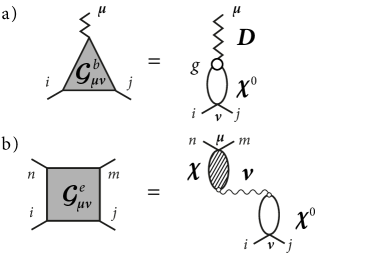
Figure 2: (a) Mixed Green’s function $\mathcal{G}^{b}$ from the approximated Baym functional in Eq. (30); (b) Two-particle Green’s function $\mathcal{G}^{e}=\mathcal{G}^{ee}$ for $GW$, $T^{ph}$ and $T^{pp}$.

Let us now discuss the 2-GF $\mathcal{G}^{e}$. The functional $\tilde{\Phi}$ in Eq. (30) is independent of the Coulomb interaction $v$ and therefore $\mathcal{G}^{eb}=0$, or equivalently $\mathcal{G}^{e}=\mathcal{G}^{ee}$, see Eq. (24). For $\mathcal{G}^{ee}$ we consider a large class of perturbative and nonperturbative approximations like the second-Born (2B), $GW$ and $T$-matrix in the particle-hole ($T^{ph}$) and particle-particle ($T^{pp}$) channels as well as $GW$ plus exchange ($X$), $T^{ph}+X$ and $T^{pp}+X$ [47]. In Ref. [47] we have also shown how to include three-particle correlations through a generalization of the GKBA to the three-particle Green’s function. The method has been dubbed the Faddeev approach and it is particularly suited to study the correlated electron dynamics in molecules after an inner-valence ionization. All the aforementioned approximations to $\mathcal{G}^{ee}$ satisfy the symmetry condition in Eq. (29); hence the resulting theory is fully conserving.

For the more familiar $GW$, $T^{ph}$ and $T^{pp}$ approximations the 2-GF satisfies an RPA-like equation whose diagrammatic representation can be found in, e.g., Figure 1 of Ref. [47]. Therefore, the 2-GF can be written as (in matrix form)

$$\bm{\mathcal{G}}^{ee}(t) =-i\int^{t}\!\!dt^{\prime}\Big{\{}\bm{\mathit{\chi}}^{>}(t,t^{\prime})\mathbfit{v}(t^{\prime})\bm{\mathit{\chi}}^{0,<}(t^{\prime},t)-(>\leftrightarrow<)\Big{\}},$$ (36)

where

$$\bm{\mathit{\chi}}^{\lessgtr}=(\mbox{\boldmath$\delta$}+\bm{\mathit{\chi}}^{R}\cdot\mathbfit{v})\cdot\bm{\mathit{\chi}}^{0,\lessgtr}\cdot(\mathbfit{v}\cdot\bm{\mathit{\chi}}^{A}+\mbox{\boldmath$\delta$})$$ (37)

and

$$\bm{\mathit{\chi}}^{R/A} =\bm{\mathit{\chi}}^{0,R/A}+\bm{\mathit{\chi}}^{0,R/A}\cdot\mathbfit{v}\cdot\bm{\mathit{\chi}}^{R/A},$$ (38a)

$$=\bm{\mathit{\chi}}^{0,R/A}+\bm{\mathit{\chi}}^{R/A}\cdot\mathbfit{v}\cdot\bm{\mathit{\chi}}^{0,R/A}.$$ (38b)

In Eq. (37) the quantity $\delta$ stands for the Dirac delta in time and the Kroenecher delta in the two-electron space, hence for any two-time correlator $\mathcal{C}$ we have $[\mbox{\boldmath$\delta$}\cdot\mbox{\boldmath$\mathcal{C}$}](t,t^{\prime})=\int d\bar{t}\,\mbox{\boldmath$\delta$}(t-\bar{t})\mbox{\boldmath$\mathcal{C}$}(\bar{t},t^{\prime})=\mbox{\boldmath$\mathcal{C}$}(t,t^{\prime})$. Depending on the approximation the matrices in the two-electron space $\bm{\mathcal{G}}^{ee}$, $\bm{\mathit{\chi}}^{0}$ and $\mathbfit{v}$ are defined in Table 1. The perturbative 2B approximation is simply obtained by replacing the dressed $\bm{\mathit{\chi}}$ with $\bm{\mathit{\chi}}^{0}$ in Eq. (36). Notice that the matrix $\bm{\mathit{\chi}}^{0}$ in Eq. (35) coincides with the matrix $\bm{\mathit{\chi}}^{0}$ in Eq. (36) only for the 2B and $GW$ approximations. To keep the notation as light as possible we however use the same symbol even when they are different ($T^{ph}$ and $T^{pp}$ approximation) and make the reader notice the slight abuse of notation when this occurs. The diagrammatic representation of Eq. (36) is given in Fig. 2(b).

In the next section we derive the EOM for $\rho^{<}$, $\mbox{\boldmath$\gamma$}^{<}$, $\bm{\mathcal{G}}^{b}$ and $\bm{\mathcal{G}}^{ee}$ in the $GD$ approximation and in all approximations of Table 1. We also show how to modify the EOM when exchange is included and provide the diagrammatic content of the corresponding self-energies.

Table 1: Definitions of electronic two-particle tensors. The vertically grouped indices are combined into one (greek) super-index.

Quantity	$\text{2B and }GW$	$T^{pp}$	$T^{ph}$
$i\bm{\mathit{\chi}}_{\begin{subarray}{c}13\\ 24\end{subarray}}^{0,\lessgtr}(t,t^{\prime})$	$G^{\lessgtr}_{13}(t,t^{\prime})G^{\gtrless}_{42}(t^{\prime},t)$	$-G^{\lessgtr}_{13}(t,t^{\prime})G^{\lessgtr}_{24}(t,t^{\prime})$	$-G_{13}^{\lessgtr}(t,t^{\prime})G^{\gtrless}_{42}(t^{\prime},t)$
$\bm{\mathcal{G}}^{ee}_{\begin{subarray}{c}13\\ 24\end{subarray}}$	$\mathcal{G}^{ee}_{4132}$	$\mathcal{G}^{ee}_{1234}$	$\mathcal{G}^{ee}_{1432}$
$\mathbfit{h}^{e}_{\begin{subarray}{c}13\\ 24\end{subarray}}$	$h^{e}_{13}\delta_{42}-\delta_{13}h^{e}_{42}$	$h^{e}_{13}\delta_{24}+\delta_{13}h^{e}_{24}$	$h^{e}_{13}\delta_{42}-\delta_{13}h^{e}_{42}$
$\mathbfit{v}_{\begin{subarray}{c}13\\ 24\end{subarray}}$	$v_{1432}$	$v_{1243}$	$v_{1423}$
$\bm{\rho}^{<}_{\begin{subarray}{c}13\\ 24\end{subarray}}$	$\rho^{<}_{13}\rho^{>}_{42}$	$\rho^{<}_{13}\rho^{<}_{24}$	$\rho^{<}_{13}\rho^{>}_{42}$

III GKBA+ODE scheme for NEGF simulations

III.1 GKBA for electrons and bosons

A way to close the EOM for the density matrices consists in implementing the GKBA for electrons [37] and our recently proposed GKBA for bosons [11]

$$G^{\lessgtr}(t,t^{\prime}) =-G^{R}(t,t^{\prime})\rho^{\lessgtr}(t^{\prime})+\rho^{\lessgtr}(t)G^{A}(t,t^{\prime}),$$ (45)

$$\mathbfit{D}^{\lessgtr}(t,t^{\prime}) =\mathbfit{D}^{R}(t,t^{\prime})\mbox{\boldmath$\alpha$}\mbox{\boldmath$\gamma$}^{\lessgtr}(t^{\prime})-\mbox{\boldmath$\gamma$}^{\lessgtr}(t)\mbox{\boldmath$\alpha$}\mathbfit{D}^{A}(t,t^{\prime}),$$ (46)

combined with the mean-field form of the retarded propagators:

$$G^{R}(t,t^{\prime}) =-i\theta(t-t^{\prime})T\left\{e^{-i\int_{t^{\prime}}^{t}d\tau\,h^{e}(\tau)}\right\},$$ (47)

$$\mathbfit{D}^{R}(t,t^{\prime}) =-i\mbox{\boldmath$\alpha$}\theta(t-t^{\prime})T\left\{e^{-i\int_{t^{\prime}}^{t}d\tau\,\mathbfit{h}^{b}(\tau)}\right\}.$$ (48)

We mention that more advanced propagators can be used without affecting the scaling of the numerical solution [55, 56, 57, 58, 41]. Once the GKBA is applied to a given approximation to the self-energies (or equivalently high-order Green’s functions) both $I^{e}$ and $\mathbfit{I}^{b}$ become functionals of $\rho^{<}$ and $\mbox{\boldmath$\gamma$}^{<}$; hence Eqs. (15), (17) and (19) become a closed system of integro-differential equations for the one-time unknown functions $\phi(t)$, $\rho^{<}(t)$ and $\mbox{\boldmath$\gamma$}^{<}(t)$. We refer to this approach as the GKBA+KBE.

For purely electronic systems an efficient implementation of the GKBA equation of motion (17) has been recently proposed [45, 46]. The main feature is the linear scaling with the maximum propagation time for the 2B, $GW$ and $T$-matrix approximations. In Ref. [47] the class of approximations has been further extended to include exchange effects and even three-particle correlations. The question what is the most general approximation to $\tilde{\Phi}$ for preserving the time-linear scaling property is still open. In this work we make a step in this direction and show that the approximate $\tilde{\Phi}=$ (discussed in the previous section) does not affect the overall time scaling.

III.2 GKBA form of ${\mbox{\boldmath$\mathcal{G}$}}^{b}$ and ${\mbox{\boldmath$\mathcal{G}$}}^{e}$

The Green’s functions $\bm{\mathcal{G}}^{b}$ and $\bm{\mathcal{G}}^{e}=\bm{\mathcal{G}}^{ee}$ are prerequisites for reformulating the GKBA+KBE equations in terms of first-order ODE, thus achieving a linear time-scaling scheme. The purpose of this section is to implement the GKBA and transform these high-order Green’s functions into functionals of $\rho^{<}$ and $\mbox{\boldmath$\gamma$}^{<}$.

Let us consider first $\bm{\mathcal{G}}^{b}$. Evaluating the noninteracting response functions of Eq. (35) with the GKBA in Eq. (45) we find a sum of products between matrices in the two-electron space

$$\bm{\mathit{\chi}}^{0,\lessgtr}(t,t^{\prime})=\mathbfit{P}^{R}(t,t^{\prime})\bm{\rho}^{\lessgtr}(t^{\prime})-\bm{\rho}^{\lessgtr}(t)\mathbfit{P}^{A}(t,t^{\prime}),$$ (49)

where $\mathbfit{P}^{A}(t,t^{\prime})=\left[\mathbfit{P}^{R}(t^{\prime},t)\right]^{\dagger}$ and for $t>t^{\prime}$ the particle-hole propagator fulfills the equation of motion

$$i\frac{d}{dt}\mathbfit{P}^{R}(t,t^{\prime}) =\mathbfit{h}^{e}(t)\mathbfit{P}^{R}(t,t^{\prime}),$$ (50)

with boundary condition $i\mathbfit{P}^{R}(t^{+},t)=-\mathbb{1}$ and $\mathbfit{P}^{R}(t,t^{\prime})=0$ for $t<t^{\prime}$. The boldface quantities $\bm{\rho}^{<}(t)$ and $\mathbfit{h}^{e}(t)$ are matrices in the two-electron space and they are given in Table 1 under the column 2B and $GW$. The matrix $\bm{\rho}^{>}$ is obtained from $\bm{\rho}^{<}$ by changing the one-electron matrices $\rho^{\lessgtr}\to\rho^{\gtrless}$. Substituting Eqs. (49) and (46) into Eq. (34) we find

$$\bm{\mathcal{G}}^{b}(t) =-i\int^{t}\!\!dt^{\prime}\mathbfit{D}^{R}(t,t^{\prime})\bm{\alpha}\bm{\Psi}^{b}(t^{\prime})\mathbfit{P}^{A}(t^{\prime},t),$$ (51)

with

$$\bm{\Psi}^{b}(t)\equiv\mbox{\boldmath$\gamma$}^{>}(t)\mbox{\boldmath$g$}(t)\bm{\rho}^{<}(t)-\mbox{\boldmath$\gamma$}^{<}(t)\mbox{\boldmath$g$}(t)\bm{\rho}^{>}(t).$$ (52)

Equation (51) is a functional of the bosonic and fermionic density matrices through the definitions in Table 1, Eq. (48) and Eq. (50).

Next we consider the 2-GF $\bm{\mathcal{G}}^{ee}$. Using the GKBA to evaluate the noninteracting response function $\bm{\mathit{\chi}}^{0}$ in one of the approximations of Table 1 we always find Eq. (49) where $\mathbfit{P}^{R}$ fulfills the same equation of motion as in Eq. (50) but with boundary conditions $i\mathbfit{P}^{R}(t^{+},t)=-\mathbb{1}$ for 2B and $GW$ and $i\mathbfit{P}^{R}(t^{+},t)=\mathbb{1}$ for the $T$-matrix approximations. Another important difference is that the definition of the matrices $\bm{\rho}^{\lessgtr}$ and $\mathbfit{h}^{e}(t)$ changes by changing approximation according to Table 1. Using this result the retarded and advanced noninteracting response function, i.e.,

$$\bm{\mathit{\chi}}^{0,R/A}(t,t^{\prime})\equiv\pm\theta(\pm t\mp t^{\prime})[\bm{\mathit{\chi}}^{0,>}(t,t^{\prime})-\bm{\mathit{\chi}}^{0,<}(t,t^{\prime})],$$ (53)

read

$$\bm{\mathit{\chi}}^{0,R}(t,t^{\prime}) =\mathbfit{P}^{\rm R}(t,t^{\prime})\bm{\rho}^{\Delta}(t^{\prime}),$$ (54a)

$$\bm{\mathit{\chi}}^{0,A}(t,t^{\prime}) =\bm{\rho}^{\Delta}(t)\mathbfit{P}^{\rm A}(t,t^{\prime}).$$ (54b)

where

$$\bm{\rho}^{\Delta}(t) \equiv\bm{\rho}^{>}(t)-\bm{\rho}^{<}(t).$$ (55)

In Ref. [47] we have shown that inserting Eqs. (54) into Eq. (38) for $\bm{\mathit{\chi}}^{R/A}$ and then using Eq. (49) for $\bm{\mathit{\chi}}^{0,\lessgtr}$, the lesser/greater interacting response function in Eq. (37) can be written as

$$\bm{\mathit{\chi}}^{\lessgtr}=\bm{\Pi}^{R}\bm{\rho}^{\lessgtr}\cdot\big{(}\mbox{\boldmath$\delta$}+\mathbfit{v}\bm{\rho}^{\Delta}\bm{\Pi}^{A}\big{)}-\big{(}\mbox{\boldmath$\delta$}+\bm{\Pi}^{R}\bm{\rho}^{\Delta}\mathbfit{v}\big{)}\cdot\bm{\rho}^{\lessgtr}\bm{\Pi}^{A},$$ (56)

where the dressed propagator $\bm{\Pi}^{R}(t,t^{\prime})=\left[\bm{\Pi}^{A}(t^{\prime},t)\right]^{\dagger}$ fulfills the RPA equation

$$\bm{\Pi}^{R}-\mathbfit{P}^{R} =\bm{\Pi}^{R}\cdot\bm{\rho}^{\Delta}\mathbfit{v}\mathbfit{P}^{R}=\mathbfit{P}^{R}\bm{\rho}^{\Delta}\mathbfit{v}\cdot\bm{\Pi}^{R},$$ (57a)

$$\bm{\Pi}^{A}-\mathbfit{P}^{A} =\bm{\Pi}^{A}\cdot\mathbfit{v}\bm{\rho}^{\Delta}\mathbfit{P}^{A}=\mathbfit{P}^{A}\mathbfit{v}\bm{\rho}^{\Delta}\cdot\bm{\Pi}^{A}.$$ (57b)

For later purposes we also observe that taking into account the equation of motion (50) for $\mathbfit{P}^{R}$ together with its boundary condition, the dressed propagators satisfy a simple EOM

$$i\frac{d}{dt}\bm{\Pi}^{R}(t,t^{\prime}) =\big{[}\mathbfit{h}^{e}(t)+a\,\bm{\rho}^{\Delta}(t)\mathbfit{v}(t)\big{]}\bm{\Pi}^{R}(t,t^{\prime}),$$ (58a)

$$-i\frac{d}{dt}\bm{\Pi}^{A}(t^{\prime},t) =\bm{\Pi}^{A}(t^{\prime},t)\big{[}\mathbfit{h}^{e}(t)+a\,\mathbfit{v}(t)\bm{\rho}^{\Delta}(t)\big{]},$$ (58b)

where the constant $a$ depends on the approximation: $a=0$ in 2B, $a=-1$ in $GW$, $a=1$ in $T^{ph},\;T^{pp}$. The two-time function $\bm{\Pi}^{R}$ can be interpreted as a dressed particle-hole (for $GW$ and $T^{ph}$) or particle-particle (for $T^{pp}$) propagator.

We have now all the ingredients to obtain the GKBA form of the 2-GF, and hence to transform $\bm{\mathcal{G}}^{ee}$ into a functional of $\rho^{<}$. We substitute Eq. (56) for $\mbox{\boldmath$\chi$}^{\lessgtr}$ and Eq. (49) for $\mbox{\boldmath$\chi$}^{0,\lessgtr}$ into Eq. (36) and find

$$\bm{\mathcal{G}}^{ee}(t) =i\Big{[}\Big{(}\underbrace{\bm{\Pi}^{R}\bm{\rho}^{>}\cdot(\mbox{\boldmath$\delta$}+\mathbfit{v}\,\bm{\rho}^{\Delta}\bm{\Pi}^{A})-(\mbox{\boldmath$\delta$}+\bm{\Pi}^{R}\bm{\rho}^{\Delta}\,\mathbfit{v})\cdot\bm{\rho}^{>}\bm{\Pi}^{\rm A}}_{\mbox{\boldmath$\chi$}^{>}}\Big{)}\cdot\mathbfit{v}\underbrace{\bm{\rho}^{<}\mathbfit{P}^{A}}_{-\mbox{\boldmath$\chi$}^{0,<}}\Big{]}(t,t)-\Big{[}>\;\leftrightarrow\;<\Big{]}(t,t)$$

$$=i\Big{[}\bm{\Pi}^{R}\bm{\rho}^{>}\mathbfit{v}\bm{\rho}^{<}\cdot\mathbfit{P}^{A}+\bm{\Pi}^{R}(\bm{\rho}^{>}\mathbfit{v}\bm{\rho}^{\Delta}-\bm{\rho}^{\Delta}\mathbfit{v}\bm{\rho}^{>})\cdot\bm{\Pi}^{\rm A}\cdot\mathbfit{v}\bm{\rho}^{<}\mathbfit{P}^{A}\Big{]}(t,t)$$

$$-i\Big{[}\bm{\Pi}^{R}\bm{\rho}^{<}\mathbfit{v}\bm{\rho}^{>}\cdot\mathbfit{P}^{A}+\bm{\Pi}^{R}(\bm{\rho}^{<}\mathbfit{v}\bm{\rho}^{\Delta}-\bm{\rho}^{\Delta}\mathbfit{v}\bm{\rho}^{<})\cdot\bm{\Pi}^{A}\cdot\mathbfit{v}\bm{\rho}^{>}\mathbfit{P}^{A}\Big{]}(t,t)$$

$$=i\Big{[}\bm{\Pi}^{R}\,(\bm{\rho}^{>}\mathbfit{v}\bm{\rho}^{<}-\bm{\rho}^{<}\mathbfit{v}\bm{\rho}^{>})\cdot\mathbfit{P}^{A}+\bm{\Pi}^{R}\,(\bm{\rho}^{>}\mathbfit{v}\bm{\rho}^{<}-\bm{\rho}^{<}\mathbfit{v}\bm{\rho}^{>})\cdot\bm{\Pi}^{A}\cdot\mathbfit{v}\,\bm{\rho}^{\Delta}\mathbfit{P}^{A}\Big{]}(t,t)$$

$$=i\Big{[}\bm{\Pi}^{R}\,(\bm{\rho}^{>}\mathbfit{v}\bm{\rho}^{<}-\bm{\rho}^{<}\mathbfit{v}\bm{\rho}^{>})\cdot\bm{\Pi}^{A}\Big{]}(t,t),$$ (59)

where in the second equality we have observed that $[\bm{\Pi}^{A}\cdot\mathbfit{v}\,\bm{\rho}^{\lessgtr}\mathbfit{P}^{A}](t,t)=0$ since $\bm{\Pi}^{A}(t,\bar{t})$ contains a $\theta(\bar{t}-t)$ and $\mathbfit{P}^{A}(\bar{t},t)$ contains a $\theta(t-\bar{t})$. Making explicit the time integration we recognize the same mathematical structure of the mixed Green’s function $\bm{\mathcal{G}}^{b}$ in Eq. (51)

$$\bm{\mathcal{G}}^{ee}(t)=i\int^{t}\!dt^{\prime}\;\bm{\Pi}^{R}(t,t^{\prime})\,\bm{\Psi}^{e}(t^{\prime})\bm{\Pi}^{A}(t^{\prime},t),$$ (60)

where we have defined

$$\bm{\Psi}^{e}(t) \equiv\bm{\rho}^{>}(t)\mathbfit{v}(t)\bm{\rho}^{<}(t)-\bm{\rho}^{<}(t)\mathbfit{v}(t)\bm{\rho}^{>}(t).$$ (61)

Equation (60) is a functional of the bosonic and fermionic density matrices through the definitions in Table 1 and Eqs. (58).

III.3 EOM for ${\mbox{\boldmath$\mathcal{G}$}}^{b}$ and ${\mbox{\boldmath$\mathcal{G}$}}^{e}$

Differentiating Eq. (51) with respect to $t$ and taking into account that $\mathbfit{D}^{R}(t,t^{\prime})$ defined in Eq. (48) satisfies for $t>t^{\prime}$ the equation $i\frac{d}{dt}\mathbfit{D}^{R}(t,t^{\prime})=\mathbfit{h}^{b}(t)\mathbfit{D}^{R}(t,t^{\prime})$ we find

$$i\frac{d}{dt}\bm{\mathcal{G}}^{b}(t) =-\bm{\Psi}^{b}(t)+\mathbfit{h}^{b}(t)\bm{\mathcal{G}}^{b}(t)-\bm{\mathcal{G}}^{b}(t)\mathbfit{h}^{e}(t),$$ (62)

where we also used the equation of motion (50) for $\mathbfit{P}^{A}(t^{\prime},t)=[\mathbfit{P}^{R}(t,t^{\prime})]^{{\dagger}}$. We notice that Eq. (62) differs from the EOM in Ref. [11] for the minus sign in front of $\bm{\Psi}^{b}$. This is due to the fact that a minus sign has been introduced in the present definition of $\rho^{>}$, see Eq. (13).

Similarly, differentiating Eq. (60) with respect to $t$ and taking into account the equation of motion (58) for $\bm{\Pi}^{R/A}$ we find

$$i\frac{d}{dt}\bm{\mathcal{G}}^{ee}(t)=-\bm{\Psi}^{e}(t)+\left[\mathbfit{h}^{e}(t)+a\bm{\rho}^{\Delta}(t)\mathbfit{v}(t)\right]\bm{\mathcal{G}}^{ee}(t)\\ -\bm{\mathcal{G}}^{ee}(t)\left[\mathbfit{h}^{e}(t)+a\mathbfit{v}(t)\bm{\rho}^{\Delta}(t)\right].$$ (65)

Equations (62) and (65) together with the equation of motion for $\phi(t)$ [Eq. (15)] and the equations of motion for the electronic and bosonic density matrices [Eqs. (17) and (19)], form a closed system of first-order ODE to study the dynamics of interacting electrons and bosons in a large class of approximations, see also below. This is the GKBA+ODE scheme.

Figure 3: Bosonic self-energy for electrons (a) and electronic self-energy for bosons (b).

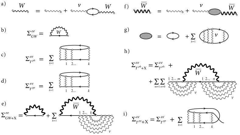
Figure 4: All possible self-energies $\Sigma^{ee}$ that can be implemented in the GKBA+ODE scheme. (a) RPA screened interaction; (b) $GW$ self-energy with RPA screened interaction; (c) $T$-matrix self-energy in the particle-hole channel; (d) $T$-matrix self-energy in the particle-particle channel; (e) $GW+X$ approximation consisting of a $GW$-like diagram and an infinite series of exchange diagrams. The screened interaction is $\bar{W}$ defined in (f) where the polarization (g) differs from the bare one as it accounts for multiples electron-hole scatterings. (h) $T^{ph}+X$ approximation consisting of the standard $T^{ph}$ diagrams and an infinite series of exchange diagrams – notice the appearance of $\bar{W}$. (i) $T^{pp}+X$ approximation.

The GKBA+ODE scheme is equivalent to the original GKBA+KBE integro-differential equations with electronic self-energy $\Sigma^{e}=\Sigma^{ee}+\Sigma^{eb}$ and bosonic self-energy $\mathbfit{\Sigma}^{b}$. For the approximate functional $\tilde{\Phi}$ in Eq. (31) we have that $\Sigma^{eb}$ is the $GD$ self-energy calculated using dressed Green’s functions $G$ and $\mathbfit{D}$, see Fig. 3(a). The dressed Green’s function $\mathbfit{D}$ differs from its equilibrium counterpart since bosons receive an electronic feedback through $\mathbfit{\Sigma}^{b}$. The latter is in turn evaluated in accordance with the $\Phi$-derivability theory of Baym and it is therefore given by the electronic bubble, see Fig. 3(b). The electronic self-energy due to the $e$-$e$ interaction $\Sigma^{ee}$ can instead be approximated in several ways. In addition to the perturbative 2B approximation [which corresponds to set $a=0$ in Eq. (65)] the two-electron index-order outlined in Table 1 is equivalent to the implementation of the $GW$ approximation ($a=-1$), see Fig. 4(a, b) or the $T$-matrix approximation ($a=1$) in the particle-hole and particle-particle channels, see Fig. 4(c,d).

The 2-GF in the $GW$ and $T$-matrix approximations solve the Bethe-Salpeter equation (BSE) with kernel $\mathbfit{v}$ given in Table 1 under the respective ($GW$ or $T^{ph}$) column. Exchange effects to all orders can be included using the kernel $\mathbfit{w}$ (same index-order convention as $\mathbfit{v}$) where

$$w_{imnj}=v_{imnj}-v_{imjn},$$ (66)

i.e., the sum of the direct and exchange ($X$) Coulomb integrals. The addition of exchange to the BSE kernel preserves the symmetry condition in Eq. (29) and, therefore, these approximations too are conserving. The GKBA form of the resulting $\bm{\mathcal{G}}^{ee}$ satisfies Eq. (65) where all $\mathbfit{v}$’s are replaced by $\mathbfit{w}$ – hence also the definition of $\bm{\Psi}^{e}$ in Eq. (61) changes. We refer to these approximations as the $GW+X$ method if $\mathbfit{w}$ is written with the $GW$ index-order and the $T^{ph}+X$ method if $\mathbfit{w}$ is written in the $T^{ph}$ index-order [47]. As there is a one-to-one diagrammatic correspondence between $\mathcal{G}^{ee}$ and $\Sigma^{ee}$ it is instructive to work out the self-energy diagrams in these two approximations. We anticipate that $\Sigma^{ee}$ is not $\Phi$-derivable in $GW+X$ and $T^{ph}+X$ (nonetheless the theory is conserving).

In Fig. 4(e) we show the $GW+X$ self-energy. It consists of a $GW$-like diagram and of an infinite series of exchange diagrams. The screened interaction $\bar{W}$ differs from the RPA $W$ in Fig. 4(a) since the polarization contains a nonperturbative vertex correction describing the multiple scattering between an electron-hole pair, see Fig. 4(f, g). If we replace $\bar{W}$ with the RPA $W$ and restrict the sum over $k$ to $k=1$ then the $GW+X$ self-energy reduces to the SOSEX self-energy introduced in Ref. [59], see also Refs. [60, 61, 62].

The $T^{ph}+X$ self-energy is illustrated in Fig. 4(h). In addition to the standard $T^{ph}$ diagrams, see again Fig. 4(d), this approximation contains a $GW$-like diagram decorated by an infinite series of exchange terms at both vertices. It is worth noticing that the sum over the interactions start from unity on the left and from zero on the right, hence no $GW$-like diagram is contained in here. Interestingly, the screened interaction is the same as in the $GW+X$ approximations, i.e., it is the $\bar{W}$ of Fig. 4(f). We finally observe that the Bethe-Salpeter equation with kernel $\mathbfit{w}$ in the particle-particle channel would lead to a multiple counting of the same diagram since exchanging two particles twice is equivalent to no exchange. Therefore the proper way of constructing the $T^{pp}+X$ approximation is depicted in Fig. 4(i), where all internal lines are bare $e$-$e$ interactions. The EOM for $\bm{\mathcal{G}}^{ee}$ in $T^{pp}+X$ is the same as in the $T^{pp}$ approximation. The difference appears in the EOM for $\rho^{<}$; the collision integral $I^{ee}$ of Eq. (25a) should in this case be calculated with $v_{imnj}\to w_{imnj}$.

As Fig. 4 shows, the GKBA+ODE scheme can be implemented for a large number of methods. For all of them the EOM have the same mathematical structure:

$$i\frac{d}{dt}\phi_{\mu}(t) =h^{b}_{\mu\nu}(t)\phi_{\nu}(t)+\sum\nolimits_{ij}\bar{g}_{\mu,ij}\rho_{ji}(t),$$ (67a)

$$i\frac{d}{dt}\rho^{<}_{lj}(t) =\big{[}h^{e}(t),\rho^{<}(t)\big{]}_{lj}+\left(-c\sum_{imn}\big{(}v_{lnmi}(t)-x^{\prime}\,v_{lnim}(t)\big{)}\mathcal{G}^{ee}_{imjn}(t)+d\sum_{\mu,i}g_{\mu,li}(t)\,\mathcal{G}^{b}_{\mu,ij}(t)-(l\leftrightarrow j)^{\ast}\right),$$ (67b)

$$i\frac{d}{dt}\gamma_{\mu\nu}^{<}(t) =\big{[}\mathbfit{h}^{b}(t),\mbox{\boldmath$\gamma$}^{<}(t)\big{]}_{\mu\nu}+\left(d\sum_{mn}\bar{g}_{\mu,mn}(t)\,\mathcal{G}^{b}_{\nu,nm}(t)-(\mu\leftrightarrow\nu)^{\ast}\right),$$ (67c)

$$i\frac{d}{dt}\bm{\mathcal{G}}^{b}(t) =-\bm{\Psi}^{b}(t)+\mathbfit{h}^{b}(t)\,\bm{\mathcal{G}}^{b}(t)-\bm{\mathcal{G}}^{b}(t)\,\mathbfit{h}^{e}(t),$$ (67d)

$$i\frac{d}{dt}\bm{\mathcal{G}}^{ee}(t) =-\bm{\Psi}^{e}(t)+\left[\mathbfit{h}^{e}(t)+a\bm{\rho}^{\Delta}(t)\,\mathbfit{u}_{x}(t)\right]\bm{\mathcal{G}}^{ee}(t)-\bm{\mathcal{G}}^{ee}(t)\left[\mathbfit{h}^{e}(t)+a\,\mathbfit{u}_{x}(t)\,\bm{\rho}^{\Delta}(t)\right],$$ (67e)

where the control parameters $a$, $c$, $x$, $x^{\prime}$ and $d$ allows to switch between different methods

$$\begin{aligned} &a=\left\{\begin{array}[]{rl}{\rm any}&\quad\quad{\rm HF}\\ 0&\quad\quad{\rm 2B}\\ -1&\quad\quad GW+(X)\\ 1&\quad\quad T^{ph}+(X),\;T^{pp}+(X)\end{array}\right.\end{aligned}$$

$$\begin{aligned} c=\left\{\begin{array}[]{rl}0&\quad\quad\;\;\;{\rm HF}\\ 1&\quad\quad\;\;\;{\rm otherwise}\end{array}\right.\end{aligned}$$

$$\begin{aligned} x=\left\{\begin{array}[]{rl}0&\quad\quad\;\;\;GW,\;T^{ph},\;T^{pp}+(X)\\ 1&\quad\quad\;\;\;{\rm 2B},\;GW+X,\;T^{ph}+X\end{array}\right.\end{aligned}$$

$$\begin{aligned} x^{\prime}=\left\{\begin{array}[]{rl}1&\quad\quad\;\;\;T^{pp}+X\\ 0&\quad\quad\;\;\;{\rm otherwise}\end{array}\right.\end{aligned}$$

$$\begin{aligned} d=\left\{\begin{array}[]{rl}0&\quad\quad\;\;\;{\rm Ehrenfest}\\ 1&\quad\quad\;\;\;GD\;{\rm for\;electrons},\;{\rm bubble\;for\;bosons}\end{array}\right.\end{aligned}$$

In Eq. (67e) we have introduced

$$\mathbfit{u}_{x} \equiv(1-x)\,\mathbfit{v}+x\,\mathbfit{w}$$ (68)

and

$$\bm{\Psi}^{e}(t) \equiv\bm{\rho}^{>}(t)\,\mathbfit{u}_{x}(t)\,\bm{\rho}^{<}(t)-\bm{\rho}^{<}(t)\,\mathbfit{u}_{x}(t)\,\bm{\rho}^{>}(t)$$ (69)

to distinguish $GW$ and $T^{ph}$ ($x=0$) from $GW+X$ and $T^{ph}+X$ ($x=1$). Taking into account Table 1 and the defintions of $h^{e}$, $\mathbfit{h}^{b}$ and $\bm{\Psi}^{b}$ in Eqs. (12), (14) and (52) the whole NEGF toolbox is thus equivalent to a system of five coupled first-order ODE.

Equations (67) fulfill all fundamental conservation laws and constitute the main result of this work. As with any set of first-order differential equations the GKBA+ODE scheme must be supplied with an initial condition for the unknown quantities. We could start with an uncorrelated state described by a HF electronic density matrix and no bosons, i.e.,

$$\phi_{\mu}(0) =\langle 0|\hat{\phi}_{\mu}|0\rangle,$$

$$\rho^{<}(0) =\rho^{\rm HF},$$

$$\gamma^{<}_{\mu\nu}(0) =\langle 0|\Delta\hat{\phi}_{\nu}\Delta\hat{\phi}_{\mu}|0\rangle,$$

$$\bm{\mathcal{G}}^{b} =\bm{\mathcal{G}}^{ee}=0,$$

and then switch on the couplings $v(t)$ and $g(t)$ adiabatically. At the end of the adiabatic switching the values of $\phi$, $\rho^{<}$, $\mbox{\boldmath$\gamma$}^{<}$, $\bm{\mathcal{G}}^{ee}$ and $\bm{\mathcal{G}}^{b}$ can be saved and used as the initial (correlated) conditions for the simulations of interest. However, we could also start from any initial nonequilibrium state. In paper II we implement and solve Eqs. (67) to study the dynamics of polarons and phonon-dressed doublons in the Hubbard-Holstein model starting from two different nonequilibrium initial conditions, highlighting the effects of the interplay between $e$-$e$ and $e$-$b$ interactions.

We remark that the GKBA+ODE scheme is particularly advantageous to investigate dynamical processes occurring at different time scales. Consider for instance the optical excitation in a semiconductor. Initially the dynamics is dictated by the electronic time-scale and hence the time-step to solve numerically Eqs. (67) should be kept below $\sim$ 10 attoseconds. After a while the dynamics slows down and the time-scale is dictated by the electron-phonon scattering rate. We could then stop the simulation, save the value of $\phi$, $\rho^{<}$, $\mbox{\boldmath$\gamma$}^{<}$, $\bm{\mathcal{G}}^{ee}$ and $\bm{\mathcal{G}}^{b}$, and start a second simulation using a larger time-step, e.g., $1\div 10$ femtoseconds, and the saved values as initial conditions. Alternatively, we could implement an adaptive time-step. This second option is always preferable if we have no limits to the CPU time per job.

IV Summary and outlook

In this work we developed a diagrammatic NEGF formalism to simulate the coupled electron-boson dynamics in correlated materials. The formalism relies on the GKBA for electrons [37] and on our recently proposed GKBA for bosons [11]. With the GKBAs one can collapse the KBE for the two-times Green’s functions onto integro-differential equations for the one-time density matrices. In Refs. [45, 46] it was realized that the KBE+GKBA integro-differential equations of purely electronic systems can be reformulated in terms of a system of coupled first-order ODE for the $GW$ and $T$-matrix self-energies. Shortly after such GKBA+ODE scheme was extended to include exchange effects and three-particle correlations [47]. Furthermore it was realized that a GKBA+ODE scheme can be constructed also to treat systems with only $e$-$b$ interactions [11]. Our work shows that $e$-$e$ and $e$-$b$ interactions can be treated on equal footing without altering the time-linear scaling.

We have presented a large class of methods, and for each of them the diagrammatic content of the self-energy has been explicitly worked out. The merits of the NEGF toolbox are (i) all fundamental conservation laws are satisfied independently of the method; (2) the ODE nature of the EOM allows one to address phenomena occurring at different time scales through a save-and-restart procedure accompanied by an adaptation of the time-step; (3) as a by-product of the calculation we have access to the spatially non-local correlators $\bm{\mathcal{G}}^{e}$ and $\bm{\mathcal{G}}^{b}$, containing information on charge or magnetic orders [63, 64], polaronic or polaritonic states, etc., see Ref. [65] and paper II.

The formal development of the GKBA+ODE scheme is still at its infancy. The generalization of the GKBA to higher order Green’s functions put forward in Ref. [47] may give access to even more accurate approximations while remaining within a time-linear scheme. Furthermore, the inclusion of an interaction with a fermionic or bosonic bath would make possible to simulate the dynamics of, e.g., photoionized systems [66, 67] or molecular junctions [41, 68]. Numerical works based on the GKBA+ODE scheme have begun to appear in the literature only recently [47, 48, 49]. Parallel implementations in high performance computer facilities are expected to open the door to first-principles investigations of a wide range of nonequilibrium correlated phenomena.

References

• Ziman [1960] J. M. Ziman, Electrons and Phonons: The Theory of Transport Phenomena in Solids (Oxford University Press, Oxford, 1960).
• Giustino [2017] F. Giustino, Electron-phonon interactions from first principles, Rev. Mod. Phys. 89, 015003 (2017).
• Baroni et al. [2001] S. Baroni, S. de Gironcoli, A. Dal Corso, and P. Giannozzi, Phonons and related crystal properties from density-functional perturbation theory, Rev. Mod. Phys. 73, 515 (2001).
• Verdozzi et al. [2006] C. Verdozzi, G. Stefanucci, and C.-O. Almbladh, Classical Nuclear Motion in Quantum Transport, Phys. Rev. Lett. 97, 046603 (2006).
• de Melo and Marini [2016] P. M. M. C. de Melo and A. Marini, Unified theory of quantized electrons, phonons, and photons out of equilibrium: A simplified ab initio approach based on the generalized Baym-Kadanoff ansatz, Phys. Rev. B 93, 155102 (2016).
• Konstantinova et al. [2018] T. Konstantinova, J. D. Rameau, A. H. Reid, O. Abdurazakov, L. Wu, R. Li, X. Shen, G. Gu, Y. Huang, L. Rettig, I. Avigo, M. Ligges, J. K. Freericks, A. F. Kemper, H. A. Dürr, U. Bovensiepen, P. D. Johnson, X. Wang, and Y. Zhu, Nonequilibrium electron and lattice dynamics of strongly correlated Bi2Sr2CaCu2O8+δ single crystals, Science Advances 4, eaap7427 (2018).
• Rizzi et al. [2016] V. Rizzi, T. N. Todorov, J. J. Kohanoff, and A. A. Correa, Electron-phonon thermalization in a scalable method for real-time quantum dynamics, Phys. Rev. B 93, 024306 (2016).
• van Hest et al. [2018] J. J. H. A. van Hest, G. A. Blab, H. C. Gerritsen, C. de Mello Donega, and A. Meijerink, The role of a phonon bottleneck in relaxation processes for ln-doped nayf4 nanocrystals, The Journal of Physical Chemistry C 122, 3985 (2018).
• Ruggenthaler et al. [2018] M. Ruggenthaler, N. Tancogne-Dejean, J. Flick, H. Appel, and A. Rubio, From a quantum-electrodynamical light-matter description to novel spectroscopies, Nature Reviews Chemistry 2, 0118 (2018).
• Wang et al. [2019] L. Wang, Z. Chen, G. Liang, Y. Li, R. Lai, T. Ding, and K. Wu, Observation of a phonon bottleneck in copper-doped colloidal quantum dots, Nature Communications 10, 4532 (2019).
• Karlsson et al. [2021] D. Karlsson, R. van Leeuwen, Y. Pavlyukh, E. Perfetto, and G. Stefanucci, Fast Green’s Function Method for Ultrafast Electron-Boson Dynamics, Phys. Rev. Lett. 127, 036402 (2021).
• Mankowsky et al. [2014] R. Mankowsky, A. Subedi, M. Först, S. O. Mariager, M. Chollet, H. T. Lemke, J. S. Robinson, J. M. Glownia, M. P. Minitti, A. Frano, M. Fechner, N. A. Spaldin, T. Loew, B. Keimer, A. Georges, and A. Cavalleri, Nonlinear lattice dynamics as a basis for enhanced superconductivity in YBa2Cu3O6.5, Nature 516, 71 (2014).
• Mitrano et al. [2016] M. Mitrano, A. Cantaluppi, D. Nicoletti, S. Kaiser, A. Perucchi, S. Lupi, P. Di Pietro, D. Pontiroli, M. Riccò, S. R. Clark, D. Jaksch, and A. Cavalleri, Possible light-induced superconductivity in K3C60 at high temperature, Nature 530, 461 (2016).
• Sentef et al. [2016] M. A. Sentef, A. F. Kemper, A. Georges, and C. Kollath, Theory of light-enhanced phonon-mediated superconductivity, Phys. Rev. B 93, 144506 (2016).
• Babadi et al. [2017] M. Babadi, M. Knap, I. Martin, G. Refael, and E. Demler, Theory of parametrically amplified electron-phonon superconductivity, Phys. Rev. B 96, 014512 (2017).
• Gudmundsson et al. [2012] V. Gudmundsson, O. Jonasson, C.-S. Tang, H.-S. Goan, and A. Manolescu, Time-dependent transport of electrons through a photon cavity, Phys. Rev. B 85, 075306 (2012).
• Abdullah et al. [2018] N. R. Abdullah, C.-S. Tang, A. Manolescu, and V. Gudmundsson, Effects of photon field on heat transport through a quantum wire attached to leads, Physics Letters A 382, 199 (2018).
• Galperin [2017] M. Galperin, Photonics and spectroscopy in nanojunctions: a theoretical insight, Chem. Soc. Rev. 46, 4000 (2017).
• Chen et al. [2020] H.-Y. Chen, D. Sangalli, and M. Bernardi, Exciton-phonon interaction and relaxation times from first principles, Phys. Rev. Lett. 125, 107401 (2020).
• Stefanucci and Perfetto [2021] G. Stefanucci and E. Perfetto, From carriers and virtual excitons to exciton populations: Insights into time-resolved ARPES spectra from an exactly solvable model, Phys. Rev. B 103, 245103 (2021).
• Helmrich et al. [2021] S. Helmrich, K. Sampson, D. Huang, M. Selig, K. Hao, K. Tran, A. Achstein, C. Young, A. Knorr, E. Malic, U. Woggon, N. Owschimikow, and X. Li, Phonon-assisted intervalley scattering determines ultrafast exciton dynamics in ${\mathrm{mose}}_{2}$ bilayers, Phys. Rev. Lett. 127, 157403 (2021).
• Walther et al. [2006] H. Walther, B. T. H. Varcoe, B.-G. Englert, and T. Becker, Cavity quantum electrodynamics, Report Progrosses in Physics 69, 1325 (2006).
• Hutchison et al. [2012] J. A. Hutchison, T. Schwartz, C. Genet, E. Devaux, and T. W. Ebbesen, Modifying chemical landscapes by coupling to vacuum fields, Angewandte Chemie International Edition 51, 1592 (2012).
• Danielewicz [1984] P. Danielewicz, Quantum theory of nonequilibrium processes, I, Ann. Phys. 152, 239 (1984).
• van Leeuwen et al. [2006] R. van Leeuwen, N. Dahlen, G. Stefanucci, C.-O. Almbladh, and U. von Barth, Introduction to the Keldysh Formalism, in Time-Dependent Density Functional Theory, Lecture Notes in Physics, Vol. 706, edited by M. Marques, C. Ullrich, F. Nogueira, A. Rubio, K. Burke, and E. Gross (Springer Berlin / Heidelberg, 2006) pp. 33–59.
• Stefanucci and van Leeuwen [2013] G. Stefanucci and R. van Leeuwen, Nonequilibrium Many-Body Theory of Quantum Systems: A Modern Introduction (Cambridge University Press, Cambridge, 2013).
• Karlsson and van Leeuwen [2020] D. Karlsson and R. van Leeuwen, Non-equilibrium green’s functions for coupled fermion-boson systems, in Handbook of Materials Modeling: Methods: Theory and Modeling, edited by W. Andreoni and S. Yip (Springer International Publishing, Cham, 2020) pp. 367–395.
• Kadanoff and Baym [1962] L. Kadanoff and G. Baym, Quantum statistical mechanics Green’s function methods in equilibrium and nonequilibrium problems (W.A. Benjamin, New York, 1962).
• Kwong and Bonitz [2000] N.-H. Kwong and M. Bonitz, Real-Time Kadanoff-Baym Approach to Plasma Oscillations in a Correlated Electron Gas, Phys. Rev. Lett. 84, 1768 (2000).
• Dahlen and van Leeuwen [2007] N. E. Dahlen and R. van Leeuwen, Solving the Kadanoff-Baym Equations for Inhomogeneous Systems: Application to Atoms and Molecules, Phys. Rev. Lett. 98, 153004 (2007).
• Myöhänen et al. [2008] P. Myöhänen, A. Stan, G. Stefanucci, and R. van Leeuwen, A many-body approach to quantum transport dynamics: Initial correlations and memory effects, Eurphys. Lett. 84, 67001 (2008).
• Galperin and Tretiak [2008] M. Galperin and S. Tretiak, Linear optical response of current-carrying molecular junction: A nonequilibrium Green’s function-time-dependent density functional theory approach, J. Chem. Phys. 128, 124705 (2008).
• Myöhänen et al. [2009] P. Myöhänen, A. Stan, G. Stefanucci, and R. van Leeuwen, Kadanoff-Baym approach to quantum transport through interacting nanoscale systems: From the transient to the steady-state regime, Phys. Rev. B 80, 115107 (2009).
• von Friesen et al. [2009] M. P. von Friesen, C. Verdozzi, and C.-O. Almbladh, Successes and Failures of Kadanoff-Baym Dynamics in Hubbard Nanoclusters, Phys. Rev. Lett. 103, 176404 (2009).
• Schüler et al. [2016] M. Schüler, J. Berakdar, and Y. Pavlyukh, Time-dependent many-body treatment of electron-boson dynamics: Application to plasmon-accompanied photoemission, Phys. Rev. B 93, 054303 (2016).
• Bittner et al. [2018] N. Bittner, D. Golež, H. U. R. Strand, M. Eckstein, and P. Werner, Coupled charge and spin dynamics in a photoexcited doped Mott insulator, Phys. Rev. B 97, 235125 (2018).
• Lipavský et al. [1986] P. Lipavský, V. Špička, and B. Velický, Generalized Kadanoff-Baym ansatz for deriving quantum transport equations, Phys. Rev. B 34, 6933 (1986).
• Hermanns et al. [2014] S. Hermanns, N. Schlünzen, and M. Bonitz, Hubbard nanoclusters far from equilibrium, Phys. Rev. B 90, 125111 (2014).
• Schlünzen et al. [2016] N. Schlünzen, S. Hermanns, M. Bonitz, and C. Verdozzi, Dynamics of strongly correlated fermions: Ab initio results for two and three dimensions, Phys. Rev. B 93, 035107 (2016).
• Bar Lev and Reichman [2014] Y. Bar Lev and D. R. Reichman, Dynamics of many-body localization, Phys. Rev. B 89, 220201 (2014).
• Latini et al. [2014] S. Latini, E. Perfetto, A.-M. Uimonen, R. van Leeuwen, and G. Stefanucci, Charge dynamics in molecular junctions: Nonequilibrium Green’s function approach made fast, Phys. Rev. B 89, 075306 (2014).
• Perfetto et al. [2015] E. Perfetto, A.-M. Uimonen, R. van Leeuwen, and G. Stefanucci, First-principles nonequilibrium Green’s-function approach to transient photoabsorption: Application to atoms, Phys. Rev. A 92, 033419 (2015).
• Karlsson et al. [2018] D. Karlsson, R. van Leeuwen, E. Perfetto, and G. Stefanucci, The generalized Kadanoff-Baym ansatz with initial correlations, Phys. Rev. B 98, 115148 (2018).
• Perfetto et al. [2018] E. Perfetto, D. Sangalli, A. Marini, and G. Stefanucci, Ultrafast Charge Migration in XUV Photoexcited Phenylalanine: A First-Principles Study Based on Real-Time Nonequilibrium Green’s Functions, J. Phys. Chem. Lett. 9, 1353 (2018).
• Schlünzen et al. [2020] N. Schlünzen, J.-P. Joost, and M. Bonitz, Achieving the Scaling Limit for Nonequilibrium Green Functions Simulations, Phys. Rev. Lett. 124, 076601 (2020).
• Joost et al. [2020] J.-P. Joost, N. Schlünzen, and M. Bonitz, G1-G2 scheme: Dramatic acceleration of nonequilibrium Green functions simulations within the Hartree-Fock generalized Kadanoff-Baym ansatz, Phys. Rev. B 101, 245101 (2020).
• Pavlyukh et al. [2021] Y. Pavlyukh, E. Perfetto, and G. Stefanucci, Photoinduced dynamics of organic molecules using nonequilibrium Green’s functions with second-Born, GW, T-matrix, and three-particle correlations, Phys. Rev. B 104, 035124 (2021).
• Perfetto et al. [2021] E. Perfetto, Y. Pavlyukh, and G. Stefanucci, Real-time $GW$: ab initio description of the ultrafast carrier and exciton dynamics in two-dimensional systems, arXiv:2109.15209  (2021).
• Borkowski et al. [2021] L. Borkowski, N. Schlünzen, J. P. Joost, F. Reiser, and M. Bonitz, Doublon production in correlated materials by multiple ion impacts, arXiv:2110.06644  (2021).
• Baym and Kadanoff [1961] G. Baym and L. P. Kadanoff, Conservation Laws and Correlation Functions, Phys. Rev. 124, 287 (1961).
• Baym [1962] G. Baym, Self-Consistent Approximations in Many-Body Systems, Phys. Rev. 127, 1391 (1962).
• Säkkinen [2016] N. Säkkinen, Application of time-dependent many-body perturbation theory to excitation spectra of selected finite model systemsPh.D. thesis, University of Jyväskylä (2016).
• Pellegrini et al. [2015] C. Pellegrini, J. Flick, I. V. Tokatly, H. Appel, and A. Rubio, Optimized Effective Potential for Quantum Electrodynamical Time-Dependent Density Functional Theory, Phys. Rev. Lett. 115, 093001 (2015).
• Fan [1951] H. Y. Fan, Temperature Dependence of the Energy Gap in Semiconductors, Phys. Rev. 82, 900 (1951).
• Marini [2008] A. Marini, Ab Initio Finite-Temperature Excitons, Phys. Rev. Lett. 101, 106405 (2008).
• Marini and Del Sole [2003] A. Marini and R. Del Sole, Dynamical Excitonic Effects in Metals and Semiconductors, Phys. Rev. Lett. 91, 176402 (2003).
• Haug [1992] H. Haug, Interband Quantum Kinetics with LO-Phonon Scattering in a Laser-Pulse-Excited Semiconductor I. Theory, Phys. Status Solidi B 173, 139 (1992).
• Bonitz et al. [1999] M. Bonitz, D. Semkat, and H. Haug, Non-Lorentzian spectral functions for Coulomb quantum kinetics, Eur. Phys. J. B 9, 309 (1999).
• Ren et al. [2015] X. Ren, N. Marom, F. Caruso, M. Scheffler, and P. Rinke, Beyond the GW approximation: A second-order screened exchange correction, Phys. Rev. B 92, 081104(R) (2015).
• Maggio and Kresse [2017] E. Maggio and G. Kresse, GW Vertex Corrected Calculations for Molecular Systems, J. Chem. Theory Comput. 13, 4765 (2017).
• Pavlyukh et al. [2020] Y. Pavlyukh, G. Stefanucci, and R. van Leeuwen, Dynamically screened vertex correction to GWPhys. Rev. B 102, 045121 (2020).
• Wang et al. [2021] Y. Wang, P. Rinke, and X. Ren, Assessing the G${}_{\textrm{0}}$W${}_{\textrm{0}}$ $\gamma$ ${}_{\textrm{0}}$ ${}^{\textrm{(1)}}$ Approach: Beyond G${}_{\textrm{0}}$W${}_{\textrm{0}}$ with Hedin’s Full Second-Order Self-Energy Contribution, J. Chem. Theory Comput. 17, 5140 (2021).
• Tuovinen et al. [2019] R. Tuovinen, D. Golež, M. Schüler, P. Werner, M. Eckstein, and M. A. Sentef, Adiabatic Preparation of a Correlated Symmetry‐Broken Initial State with the Generalized Kadanoff-Baym Ansatz, Phys. Status Solidi B 256, 1800469 (2019).
• Tuovinen et al. [2020] R. Tuovinen, D. Golež, M. Eckstein, and M. A. Sentef, Comparing the generalized Kadanoff-Baym ansatz with the full Kadanoff-Baym equations for an excitonic insulator out of equilibrium, Phys. Rev. B 102, 115157 (2020).
• Fehske et al. [2011] H. Fehske, G. Wellein, and A. R. Bishop, Spatiotemporal evolution of polaronic states in finite quantum systems, Phys. Rev. B 83, 075104 (2011).
• Perfetto et al. [2020] E. Perfetto, A. Trabattoni, F. Calegari, M. Nisoli, A. Marini, and G. Stefanucci, Ultrafast Quantum Interference in the Charge Migration of Tryptophan, J. Phys. Chem. Lett. , 9 (2020).
• Månsson et al. [2021] E. P. Månsson, S. Latini, F. Covito, V. Wanie, M. Galli, E. Perfetto, G. Stefanucci, H. Hübener, U. De Giovannini, M. C. Castrovilli, A. Trabattoni, F. Frassetto, L. Poletto, J. B. Greenwood, F. Légaré, M. Nisoli, A. Rubio, and F. Calegari, Real-time observation of a correlation-driven sub 3 fs charge migration in ionised adenine, Communications Chemistry 4, 73 (2021).
• Tuovinen et al. [2021] R. Tuovinen, R. van Leeuwen, E. Perfetto, and G. Stefanucci, Electronic transport in molecular junctions: The generalized Kadanoff-Baym ansatz with initial contact and correlations, J. Chem. Phys. 154, 094104 (2021).