Implicit vs Unfolded Graph Neural Networks

Abstract

It has been observed that graph neural networks (GNN) sometimes struggle to maintain a healthy balance between the efficient modeling long-range dependencies across nodes while avoiding unintended consequences such oversmoothed node representations or sensitivity to spurious edges. To address this issue (among other things), two separate strategies have recently been proposed, namely implicit and unfolded GNNs. The former treats node representations as the fixed points of a deep equilibrium model that can efficiently facilitate arbitrary implicit propagation across the graph with a fixed memory footprint. In contrast, the latter involves treating graph propagation as unfolded descent iterations as applied to some graph-regularized energy function. While motivated differently, in this paper we carefully quantify explicit situations where the solutions they produce are equivalent and others where their properties sharply diverge. This includes the analysis of convergence, representational capacity, and interpretability. In support of this analysis, we also provide empirical head-to-head comparisons across multiple synthetic and public real-world node classification benchmarks. These results indicate that while IGNN is substantially more memory-efficient, UGNN models support unique, integrated graph attention mechanisms and propagation rules that can achieve SOTA node classification accuracy across disparate regimes such as adversarially-perturbed graphs, graphs with heterophily, and graphs involving long-range dependencies.

Keywords: Graph Neural Networks, Algorithm Unfolding, Bi-level Optimization, Implicit Deep Learning, Graph Attention.

1 Introduction

Given graph data with node features, graph neural networks (GNNs) represent an effective way of exploiting relationships among these features to predict labeled quantities of interest, e.g., node classification (Wu et al., 2020; Zhou et al., 2018). In particular, each layer of a message-passing GNN is constructed by bundling a graph propagation step with an aggregation function such that information can be shared between neighboring nodes to an extent determined by network depth. (Kipf and Welling, 2017; Hamilton et al., 2017; Kearnes et al., 2016; Velickovic et al., 2018).

For sparsely-labeled graphs, or graphs with entity relations reflecting long-range dependencies, it is often desirable to propagate signals arbitrary distances across nodes, but without expensive memory requirements during training, oversmoothing effects (Oono and Suzuki, 2020; Li et al., 2018), or disproportionate sensitivity to bad/spurious edges (Zhu et al., 2020b, a; Zügner et al., 2019; Zügner and Günnemann, 2019). To address these issues, at least in part, two distinct strategies have recently been proposed. First, the framework of implicit deep learning (Bai et al., 2019; El Ghaoui et al., 2020) has been applied to producing supervised node embeddings that satisfy an equilibrium criteria instantiated through a graph-dependent fixed-point equation. The resulting so-called implicit GNN (IGNN) pipeline (Gu et al., 2020), as well as related antecedents (Dai et al., 2018; Gallicchio and Micheli, 2020) and descendants (Liu et al., 2021a), mimic the behavior of a GNN model with arbitrary depth for handling long-range dependencies, but is nonetheless trainable via a fixed memory budget and robust against oversmoothing effects.

Secondly, unfolded GNN (UGNN) architectures are formed via graph propagation layers patterned after the unfolded descent iterations of some graph-regularized energy function (Chen and Eldar, 2021; Liu et al., 2021b; Ma et al., 2020; Pan et al., 2021; Zhang et al., 2020; Zhu et al., 2021). In this way, the node embeddings at each UGNN layer can be interpreted as increasingly refined approximations to an interpretable energy minimizer, which can be nested within a bi-level optimization framework (Wang et al., 2016) for supervised training akin to IGNN. More broadly, similar unfolding strategies have previously been adopted for designing a variety of new deep architectures or interpreting existing ones (Geng et al., 2021; Gregor and LeCun, 2010; He et al., 2017; Hershey et al., 2014; Sprechmann et al., 2015; Veličković et al., 2020).

As such, IGNN and UGNN are closely related in the sense that their node embeddings are intentionally aligned with a meta-criterion: either a fixed-point for IGNN or an energy minimizer for UGNN, where in both cases a useful inductive bias is introduced to address similar desiderata. And yet despite these commonalities, there has thus far been no systematic examination of the meaningful similarities and differences. We take a first step in this direction via the following workflow. First, after introducing the basic setup and notation in Section 2, we overview the IGNN framework in Section 3, including its attractive reliance on memory-efficient implicit differentiation and existing convergence results. Next, Section 4 introduces a general-purpose UGNN framework that encompasses a variety of existing unfolded models as special cases, including models with graph attention, broad graph propagation operators, and nonlinear activation functions. Sections 5–7 provide comparative analysis of the relative strengths and weaknesses of IGNN and UGNN models with respect to convergence guarantees, model expressiveness, and robustness via integrated graph attention mechanisms. We conclude with empirical comparisons in Section 8, while proofs and additional experiments and details are deferred to the appendices.

Overall, our contributions can be summarized as follows:

• Although the original conceptions are unique, we consider a sufficiently broad design space of IGNN and UGNN models such that practically-relevant, interpretable regions of exact overlap can be established, analyzed, and contrasted with key areas of nonconformity.

• Within this framework, we compare the relative ability of IGNNs and UGNNs to converge to optimal (or locally-optimal) solutions per various model-specific design criteria. Among other things, this analysis reveals that IGNNs enjoy an advantage in that (unlike UGNNs) their implicit layers do not unavoidably induce symmetric propagation weights. In contrast, we show that UGNNs are more flexible by accommodating a broader class of robust nonlinear graph propagation operators while still guaranteeing at least local convergence.

• We investigate the consequences of symmetric (layer-tied) UGNN propagation weights. In particular, we prove that with linear activations, a UGNN can reproduce any IGNN representation, and define sufficient conditions for equivalency in broader regimes. We also show that UGNN layers with symmetric, layer-tied weights can exactly mimic arbitrary graph convolutional network (GCN) models (Kipf and Welling, 2017) characterized by asymmetric, layer-specific weights without introducing any additional parameters or significant complexity. Collectively, these results suggest that the weight symmetry enforced by UGNN models may not be overly restrictive in practice.

• We demonstrate that, unlike IGNN, UGNN can naturally support a novel nonlinear graph attention mechanism that is explicitly anchored to an underlying end-to-end energy function, contributing stability with respect to edge uncertainty without introducing additional parameters or design heuristics. This capability is relevant to handling graphs with heterophily (meaning nearby nodes may not share similar labels and/or features) and adversarial perturbations.

• Empirically, we provide the comprehensive, head-to-head comparisons between equivalently-sized IGNN and UGNN models while evaluating computational complexity and memory costs. These results also serve to complement our analytical findings while showcasing node classification regimes whereby IGNN or UGNN can achieve SOTA performance in terms of either accuracy or efficiency.

We note that portions of this work have appeared previously in (Yang et al., 2021); however, no detailed comparison with IGNN, comprehensive convergence guarantees to generalized fixed points, or analysis of model expressiveness were considered.

2 Basic Setup

Consider a graph ${\mathcal{G}}=\{{\mathcal{V}},{\mathcal{E}}\}$, with $n=|{\mathcal{V}}|$ nodes and $m=|{\mathcal{E}}|$ edges. We define $L\in\mathbb{R}^{n\times n}$ as the Laplacian of ${\mathcal{G}}$, meaning $L=D-A=B^{\top}B$, where $D$ and $A$ are degree and adjacency matrices respectively, while $B\in\mathbb{R}^{m\times n}$ is an incidence matrix. We also let $\widetilde{A}=A+I$ (i.e., $A$ with self loops) and denote $\widetilde{D}$ as the corresponding degree matrix.

Both IGNNs and UGNNs incorporate graph structure via optimized embeddings $Y^{*}\in\mathbb{R}^{n\times d}$ that are a function of some adjustable weights ${\mathcal{W}}$, i.e., $Y^{*}\equiv Y^{*}({\mathcal{W}})$ (for simplicity of notation, we will frequently omit including this dependency on ${\mathcal{W}}$), where by design $\partial Y^{*}({\mathcal{W}})/\partial{\mathcal{W}}$ is computable, either implicitly (IGNN) or explicitly (UGNN). We may then insert these embeddings within an application-specific meta-loss given by

$$\ell_{\theta}\left(\theta,{\mathcal{W}}\right)\triangleq\sum_{i=1}^{n^{\prime}}{\mathcal{D}}\big{(}g\left[\mbox{\boldmath$y$}_{i}^{*}({\mathcal{W}});\theta\right],\mbox{\boldmath$t$}_{i}\big{)},$$ (1)

where $g:\mathbb{R}^{d}\rightarrow\mathbb{R}^{c}$ is some differentiable node-wise function with parameters $\theta$ and $c$-dimensional output tasked with predicting ground-truth node-wise targets $\mbox{\boldmath$t$}_{i}\in\mathbb{R}^{c}$. Additionally, $\mbox{\boldmath$y$}_{i}^{*}({\mathcal{W}})$ is the $i$-th row of $Y^{*}({\mathcal{W}})$, $n^{\prime}<n$ is the number of labeled nodes (we assume w.l.o.g. that the first $n^{\prime}$ nodes are labeled), and ${\mathcal{D}}$ is a discriminator function, e.g., cross-entropy for classification, squared error for regression, etc. Given that $Y^{*}({\mathcal{W}})$ is differentiable by construction, we can optimize $\ell_{\theta}\left(\theta,{\mathcal{W}}\right)$ via gradient descent to obtain our final predictive model.

At a conceptual level then, the only difference between IGNNs and UGNNs is in how the corresponding optimal embeddings $Y^{*}({\mathcal{W}})$ are motivated and computed. We introduce the specifics of each option in the following two sections.

3 Overview of Implicit GNNs

IGNN models are predicated on the fixed-point update

$$Y^{(k+1)}=\sigma\left[PY^{(k)}W_{p}+f\left(X;W_{x}\right)\right],$$ (2)

where $Y^{(k)}$ are node embeddings after the $k$-th iteration, ${\mathcal{W}}=\{W_{p},W_{x}\}$ is a set of two weight matrices, $P\in\mathbb{R}^{n\times n}$ is an arbitrary graph propagation operator (e.g., $P=A$), and $\sigma$ is a nonlinear activation function. Additionally, $f:\mathbb{R}^{n\times d_{0}}\rightarrow\mathbb{R}^{n\times d}$ is a base predictor function that converts the initial $d_{0}$-dimensional node features $X\in\mathbb{R}^{n\times d_{0}}$ into $d$-dimensional candidate embeddings, e.g., $f\left(X;W_{x}\right)=XW_{x}$ or $f\left(X;W_{x}\right)=\mbox{MLP}\left[X;W_{x}\right]$.

Now assume that $\sigma$ is a differentiable component-wise non-expansive (CONE) mapping as specified in (Gu et al., 2020). This condition stipulates that $\sigma$ applies the same function individually to each element of its input, and that this function satisfies $\|x-y\|\geq\|\sigma(x)-\sigma(y)\|$ for all $\{x,y\}\in\mathbb{R}^{2}$ (with some abuse of notation, we will overload the definition of $\sigma$ when the meaning is clear from context). Furthermore, we assume that the weights $W_{p}$ are such that $\lambda_{\tiny\mbox{pf}}(|P\otimes W_{p}|)<1$, where $|\cdot|$ denotes the element-wise absolute value and $\lambda_{\tiny\mbox{pf}}$ refers to the Peron-Frobenius eigenvalue.

Under these conditions, it has been shown in (Gu et al., 2020) that $\lim_{k\rightarrow\infty}Y^{(k)}=Y^{*}$, where $Y^{*}$ satisfies the fixed-point equation $Y^{*}=\sigma\left[PY^{*}W_{p}+f\left(X;W_{x}\right)\right]$. Therefore, as an IGNN forward pass we can iterate (2) $K$ times, where $K$ is sufficiently large, to compute node embeddings $Y^{(K)}\approx Y^{*}$ for use within the meta-loss from (1). For the IGNN backward pass, implicit differentiation methods (Bai et al., 2019; El Ghaoui et al., 2020), carefully tailored for handling graph-based models (Gu et al., 2020), can but used to compute gradients of $Y^{*}$ with respect to $W_{p}$ and $W_{x}$. Critically, this implicit technique does not require storing each intermediate representation $\{Y^{(k)}\}_{k=1}^{K}$ from the forward pass, and hence is quite memory efficient even if $K$ is arbitrarily large. As $K$ can be viewed as quantifying the extent of signal propagation across the graph, IGNNs can naturally capture long-range dependencies with a $K$-independent memory budget unlike more traditional techniques.

In follow-up work from (Liu et al., 2021a) a special case of (2) is considered whereby $\sigma$ is an identity mapping and $W_{p}$ is constrained to be a symmetric matrix $W_{p}^{s}$. These simplifications facilitate a more stream-lined implementation, referred to as efficient infinite-depth graph neural networks (EIGNN) in (Liu et al., 2021a), while maintaining accurate predictions on various node classification tasks. Additionally, as we will demonstrate in the next section, the EIGNN fixed point minimizes an explicit energy function allowing this approach to be simultaneously interpreted as a special case of UGNN as well.

4 A General-Purpose Unfolded GNN Framework

In this section we will first introduce a general-purpose energy function that, when reduced with simplifying assumptions, decomposes into various interpretable special cases that have been proposed in the literature, both as the basis for new UGNN models as well as motivation for canonical GNN architectures. Later, will describe the generic proximal gradient descent iterations designed to optimize this energy. By construction, these iterations unfold in one-to-one correspondence with the UGNN model layers of each respective architecture under consideration.

4.1 Flexible Energy Function Design

Unlike IGNN models, the starting point of UGNNs is an energy function. In order to accommodate a broad variety of existing graph-regularized objectives and ultimately GNN architectures as special cases, we propose the rather general form

$$\ell_{Y}(Y;{\mathcal{W}},f,\rho,\widetilde{B},\phi)\triangleq\left\|Y-f\left(X;W_{x}\right)\right\|_{W_{f}}^{2}+\sum_{i=1}^{m}\rho\left(\left[\widetilde{B}YW_{p}Y^{\top}\widetilde{B}^{\top}\right]_{ii}\right)+\sum_{i=1}^{n}\phi\left(\mbox{\boldmath$y$}_{i};W_{\phi}\right),$$ (3)

where ${\mathcal{W}}=\{W_{x},W_{f},W_{p},W_{\phi}\}$ is a set of four weight matrices, $\rho:\mathbb{R}\rightarrow\mathbb{R}$ is a differentiable function, and $\widetilde{B}\in\mathbb{R}^{m\times n}$ is a function of $A$ that can be viewed as a generalized incidence matrix. Furthermore, $\phi:\mathbb{R}^{d}\rightarrow\mathbb{R}$ is an arbitrary function (possibly non-smooth) of the node embeddings that is bounded from below, and the weighted norm $\|\cdot\|_{W}$ is defined such that $\|X\|^{2}_{W}=\mbox{tr}[X^{\top}WX]$. The above loss is composed of three terms: (i) A quadratic penalty on deviations of the embeddings $Y$ from the node-wise base model $f\left(X;W_{x}\right)$, (ii) a (possibly) non-convex graph-aware penalty that favors smoothness across edges (see illustrative special cases below), and (iii) an arbitrary function of each embedding that is independent of both the graph structure $A$ and the original node features $X$.

As a representative special case, if $\widetilde{B}=B$, then the second term from (3) satisfies

$$\sum_{i=1}^{m}\rho\left(\left[\widetilde{B}YW_{p}Y^{\top}\widetilde{B}^{\top}\right]_{ii}\right)=\sum_{\{i,j\}\in{\mathcal{E}}}\rho\left(\left\|\mbox{\boldmath$y$}_{i}-\mbox{\boldmath$y$}_{j}\right\|_{W_{p}}^{2}\right),$$ (4)

which penalizes deviations between the embeddings of two nodes sharing an edge. As will be comprehensively analyzed in Section 7 below, if $\rho$ is chosen to be concave and non-decreasing on $[0,\infty)$, the resulting regularization favors robustness to bad edges, and could be useful for handling heterophily graphs or adversarial attacks. And if in addition to the assumption from (4), $\phi$ is set to zero, $\rho$ is an identity mapping, $W_{f}=I$, and $W_{p}=\lambda I$ with $\lambda>0$, then (3) collapses to the more familiar loss

$$\ell_{Y}(Y;W_{x},f)\triangleq\left\|Y-f\left(X;W_{x}\right)\right\|_{{\mathcal{F}}}^{2}+\lambda\mbox{tr}\left[Y^{\top}LY\right],$$ (5)

as originally proposed in (Zhou et al., 2004) to smooth base predictions from $f\left(X;W_{x}\right)$ using a quadratic, graph-aware regularization factor $\mbox{tr}\left[Y^{\top}LY\right]=\sum_{\{i,j\}\in{\mathcal{E}}}\left\|\mbox{\boldmath$y$}_{i}-\mbox{\boldmath$y$}_{j}\right\|^{2}$. This construction has also formed the basis of a wide variety of work linking different GNN architectures (Ma et al., 2020; Pan et al., 2021; Zhang et al., 2020; Zhu et al., 2021); more details to follow in Section 4.2.

Similarly, if we allow for broader choices of $\widetilde{B}\neq B$ with $\widetilde{L}\triangleq\widetilde{B}^{\top}\widetilde{B}=\pi(A)$ for some function $\pi:\mathbb{S}^{n}\rightarrow\mathbb{S}^{n}$ over the space of $n$-dimensional PSD matrices $\mathbb{S}^{n}$, then (5) can be generalized by swapping $L$ for this $\widetilde{L}$ as proposed in (Ioannidis et al., 2018). Candidates for $\widetilde{L}$ include normalized graph Laplacians (Von Luxburg, 2007) and various diffusion kernels (Klicpera et al., 2019b) designed according to application-specific requirements, e.g., graph signal denoising. Moreover, if we reintroduce $W_{p}\neq I$, then it can be shown that the EIGNN fixed point (assuming suitable hyperparameter settings) minimizes the resulting generalized version of (5); see Appendix for specifics of the derivation as the original EIGNN algorithm (Liu et al., 2021a) is not motivated in this way .

4.2 Descent Iterations That Form UGNN Layers

We now derive descent iterations for the general loss from the previous section (and later more interpretable special cases) that will be mapped to UGNN layers. For this purpose, let $U^{(k)}$ denote a single gradient descent step along (3), excluding the possibly non-differentiable $\phi$-dependent term, and evaluated at some candidate point $Y^{(k)}$. We may compute such an abridged gradient step as

$$U^{(k)}=Y^{(k)}-\alpha\left[\widetilde{B}^{\top}\Gamma^{(k)}\widetilde{B}Y^{(k)}\left(W_{p}+W_{p}^{\top}\right)+Y^{(k)}\left(W_{f}+W_{f}^{\top}\right)-f\left(X;W\right)\right],$$ (6)

where $\alpha$ is the step size and $\Gamma^{(k)}$ is a diagonal matrix with $i$-th diagonal element given by

$$\gamma_{i}^{(k)}~{}=~{}\left.\frac{\partial\rho\left(z\right)}{\partial z}\right|_{z=\mbox{diag}\left[\widetilde{B}Y^{(k)}W_{p}\left(Y^{(k)}\right)^{\top}\widetilde{B}^{\top}\right]_{i}}.$$ (7)

We then have the following:

Lemma 1.

If $\rho$ has Lipschitz continuous gradients, then the proximal gradient update

$$Y^{(k+1)}=\mbox{prox}_{\phi}\left(U^{(k)}\right)\triangleq\arg\min_{Y}\left[\frac{1}{2\alpha}\|U^{(k)}-Y\|_{{\mathcal{F}}}^{2}+\sum_{i}\phi\left(\mbox{\boldmath$y$}_{i};W_{\phi}\right)\right],$$ (8)

is guaranteed to satisfy  $\ell_{Y}(Y^{(k+1)};{\mathcal{W}},f,\rho,\widetilde{B},\phi)\leq\ell_{Y}(Y^{(k)};{\mathcal{W}},f,\rho,\widetilde{B},\phi)$  for any $\alpha\in\left(0,1/{\mathcal{L}}\right]$, where ${\mathcal{L}}$ is the Lipschitz constant for gradients of (3) w.r.t. $Y$, excluding the non-smooth $\phi$ term.

The function $\mbox{prox}_{\phi}:\mathbb{R}^{d}\rightarrow\mathbb{R}^{d}$ is known as the proximal operator associated with $\phi$ (separably extended across all $n$ nodes in the graph), and the proof follows from basic properties of gradient descent (Bertsekas, 1999) and proximal methods (Combettes and Pesquet, 2011); see Appendix.

Generally speaking, the mapping $Y^{(k)}\mapsto U^{(k)}$ from (6) can be viewed as a (possibly nonlinear) graph filter, while $\mbox{prox}_{\phi}$ from (8) serves as an activation function applied to the embedding of each node. Collectively then, $Y^{(k+1)}=\mbox{prox}_{\phi}\left(U^{(k)}\right)$ provides a flexible template for UGNN layers that naturally reduces to common GNN architectures per various design choices. And analogous to IGNN, we can execute $K$ UGNN steps to approximate some $Y^{*}$, which could be a fixed-point, stationary point, or global optimum; more on this in Sections 4.3 and 5 below.

For example, consider the selection $\sum_{i}\phi\left(\mbox{\boldmath$y$}_{i};W_{\phi}\right)=\sum_{i,j}{\mathcal{I}}_{\infty}[y_{ij}<0]$, where $y_{ij}$ is the $(i,j)$-th element of $Y$ and ${\mathcal{I}}_{\infty}$ is an indicator function that assigns an infinite penalty to any $y_{ij}<0$. The proximal operator then becomes $\mbox{prox}_{\phi}(U)=\mbox{ReLU}(U)$, i.e., a ReLU function that element-wise sets negative values to zero. If we add this $\phi$-dependent term to (5) (as a special case of (3)), the resulting update becomes

$$Y^{(k+1)}=\mbox{prox}_{\phi}\left(U^{(k)}\right)=\mbox{ReLU}\left(Y^{(k)}-\alpha\left[\left(\lambda L+I\right)Y^{(k)}-f\left(X;W\right)\right]\right).$$ (9)

And when combined with observations from (Ma et al., 2020; Pan et al., 2021; Zhang et al., 2020; Zhu et al., 2021), if we initialize with $Y^{(0)}=f\left(X;W\right)=XW$ and apply simple reparameterizations, the first iteration reduces to the canonical GCN layer $Y^{(1)}=\mbox{ReLU}\left[\widetilde{D}^{-1/2}\widetilde{A}\widetilde{D}^{-1/2}XW\right]$ from (Kipf and Welling, 2017). Subsequent iterations are no longer equivalent, although the inherent differences (e.g., the skip connections from the input layer) are useful for avoiding oversmoothing effects that can at times hamper deep GCN models (Oono and Suzuki, 2020; Li et al., 2018; Rong et al., 2020).

Additionally, the widely-used APPNP architecture (Klicpera et al., 2019a) is also a special case of (9) when the ReLU operator is removed (i.e., $\phi$ is zero), $\alpha=\frac{1}{1+\lambda}$, and $L$ is changed to the symmetric normalized Laplacian (Von Luxburg, 2007). And as a final representative example, if we adopt a nonlinear choice for $\rho$, then $L$ in (9) will be replaced by $L^{(k)}\triangleq B^{\top}\Gamma^{(k)}B$, where $\Gamma^{(k)}$ rescales graph edges. As will be discussed in much more depth in Section 7, this instantiates a form of graph attention, whereby the attention weights produced by a concave, non-decreasing $\rho$ add robustness to spurious edges.

4.3 UGNN Fixed Points and Connections with IGNN

While UGNN layers are formed from the descent steps of a graph-regularized energy, for a more direct comparison with IGNN, it is illuminating to consider the situation where the update $Y^{(k+1)}=\mbox{prox}_{\phi}\left(U^{(k)}\right)$ is iterated with $k$ becoming sufficiently large. In this case, we may ideally reach a fixed point $Y^{*}$ that satisfies

$$Y^{*} = \mbox{prox}_{\phi}\left(Y^{*}-\alpha\left[\widetilde{B}^{\top}\Gamma^{*}\widetilde{B}Y^{*}\left(W_{p}+W_{p}^{\top}\right)+Y^{*}\left(W_{f}+W_{f}^{\top}\right)-f\left(X;W\right)\right]\right)$$ (10)

$$= \mbox{prox}_{\phi}\left(Y^{*}\left[I-\alpha W_{f}^{s}-\alpha W_{p}^{s}\right]+\alpha\left[I-\widetilde{B}^{\top}\Gamma^{*}\widetilde{B}\right]Y^{*}W_{p}^{s}+\alpha f\left(X;W\right)\right),$$

where $W_{p}^{s}\triangleq W_{p}+W_{p}^{\top}$ and $W_{f}^{s}\triangleq W_{f}+W_{f}^{\top}$ are symmetric weight matrices, and $\Gamma^{*}$ is defined analogously to (7). It now follows that if $W_{f}^{s}=I-W_{p}^{s},\alpha=1$ and $\Gamma^{*}=I$ (i.e., $\rho$ is an identity mapping), and we define the propagation operator as $P=I-\widetilde{B}^{\top}\widetilde{B}\equiv I-\widetilde{L}$, then (10) reduces to

$$Y^{*}=\mbox{prox}_{\phi}\left[PY^{*}W_{p}^{s}+f\left(X;W\right)\right].$$ (11)

This expression is exactly equivalent to the IGNN fixed point from Section 3 when we set $\sigma$ to the proximal operator of $\phi$ and we restrict $W_{p}$ to be symmetric. For direct head-to-head comparisons then, it is instructive to consider what CONE activation functions $\sigma$ can actually be expressed as the proximal operator of some penalty $\phi$. In this regard we have the following:

Lemma 2.

A continuous CONE function $\sigma:\mathbb{R}\to\mathbb{R}$ can be expressed as the proximal operator of some function $\phi$ iff $\sigma$ is also non-decreasing.

The proof follows from the analysis in (Gribonval and Nikolova, 2020). This result implies that, at least with respect to allowances for decreasing activation functions $\sigma$, IGNN is more flexible than UGNN.

However, the relative flexibility of IGNN vs UGNN fixed points becomes much more nuanced once we take into account convergence considerations. For example, the proximal gradient iterations from Section 4.2 do not require that $\mbox{prox}_{\phi}$ is non-expansive or CONE to guarantee descent, although it thus far remains ambiguous how this relates to obtainable fixed points of UGNN. To this end, in the next section we will evaluate when such fixed points exist, what properties they have, convergence conditions for reaching them, and importantly for present purposes, how UGNN fixed points relate to their IGNN counterparts.

5 Convergence Comparisons

In this section we first detail situations whereby convergence to a unique fixed point, that also may at times correspond with a unique UGNN global minimum, can be established. In these situations IGNN facilitates stronger guarantees in terms of broader choices for $W_{p}$ and $\sigma$. Later, we examine alternative scenarios whereby UGNN has a distinct advantage with respect to convergence guarantees to potentially local solutions.

5.1 Convergence to Unique Global Solutions

To facilitate the most direct, head-to-head comparison between IGNN and UGNN, we consider a restricted form of the UGNN energy from (3). In particular, let

$$\ell_{Y}(Y;{\mathcal{W}},f,\phi)\triangleq\left\|Y-f\left(X;W_{x}\right)\right\|_{W_{f}}^{2}+\mbox{tr}\left[Y^{\top}\widetilde{L}YW_{p}\right]+\sum_{i=1}^{n}\phi\left(\mbox{\boldmath$y$}_{i}\right),$$ (12)

which is obtainable from (3) when $\rho$ is an identity mapping and $\phi$ is assumed to have no trainable parameters. We also define $\Sigma\triangleq I\otimes W_{f}^{s}+\widetilde{L}\otimes W_{p}^{s}$, with minimum and maximum eigenvalues given by $\lambda_{\tiny\mbox{min}}(\Sigma)$ and $\lambda_{\tiny\mbox{max}}(\Sigma)$ respectively.

Theorem 3.

If $\mbox{prox}_{\phi}$ is non-expansive and $\lambda_{\tiny\mbox{min}}(\Sigma)>0$, then (12) has a unique global minimum. Additionally, starting from any initialization $Y^{(0)}$, the iterations $Y^{(k+1)}=\mbox{prox}_{\phi}\left[U^{(k)}\right]$ applied to (12) with $\alpha\in(0,2/\lambda_{\tiny\mbox{max}}(\Sigma))$ are guaranteed to converge to this global minimum as $k\rightarrow\infty$.

Corollary 4.

For any non-decreasing CONE function $\sigma$ and symmetric $W_{p}\equiv W_{p}^{s}$ satisfying $\|W_{p}^{s}\|_{2}<\|P\|_{2}^{-1}$, there will exist a function $\phi$ such that $\sigma=\mbox{prox}_{\phi}$ and the fixed point of (11) is the unique global minimum of (12) when $W_{f}$ is chosen such that $W_{f}^{s}=I-W_{p}^{s}$ and $P=I-\widetilde{L}$.

Lemma 5.

For any non-expansive $\sigma$ (not necessarily element-wise) and $W_{p}$ (not necessarily symmetric) satisfying $\|W_{p}\|_{2}<\|P\|_{2}^{-1}$, iterating (2) will converge to a unique fixed point.

Hence from Theorem 3 and Corollary 4, if we are willing to accept symmetric graph propagation weights $W_{p}^{s}$ (and a non-decreasing $\sigma$), UGNN enjoys the same convergence guarantee as IGNN, but with the added benefit of an interpretable underlying energy function. In contrast, when $W_{p}$ is not symmetric as in Lemma 5, we can only guarantee a unique IGNN fixed point, but we are no longer able to establish an association with a specific UGNN energy. In fact, it does not seem likely that any familiar/interpretable functional form can even possibly exist to underlie such a fixed point when $W_{p}$ is not symmetric. This is largely because of the following simple result:

Lemma 6.

There does not exist any second-order smooth function $h:\mathbb{R}^{n\times d}\rightarrow\mathbb{R}$ such that $\partial h(Y;W)/\partial Y=YW$ for all (asymmetric) matrices $W\in\mathbb{R}^{d\times d}$ with $d>1$ and $n\geq 1$.

And by continuity arguments, a similar result will apply to many non-smooth functions. Consequently, with asymmetric weights there is no obvious way to associate fixed points with stationary points as we have done for UGNN.

5.2 Broader Convergence Regimes

As we move to alternative energy functions with nonlinear dependencies on the graph, e.g., $\rho$ not equal to identity, meaningful (albeit possibly weaker) convergence properties for UGNN can still be established. In particular, we consider convergence to local minima, or more generally, stationary points of the underlying objective. However, because (3) may be non-convex and non-smooth, we must precisely define an applicable notion of stationarity.

While various possibilities exist, for present purposes we define $Y^{*}$ as a stationary point of (3) if ${\bf 0}\in\partial_{\tiny{\mathcal{F}}}\left[\ell_{Y}(Y^{*};{\mathcal{W}},f,\rho,\widetilde{B},\phi)\right]$, where $\partial_{\tiny{\mathcal{F}}}$ denotes the Fréchet subdifferential. The latter generalizes the standard subdifferential as defined for convex functions, to non-convex cases. More formally, the Fréchet subdifferential (Li et al., 2020a) of some function $h(Y)$ is defined as the set

$$\partial_{\tiny{\mathcal{F}}}\left[h(Y)\right]=\left\{S:h(Y)\geq h(Z)+\mbox{tr}\left[S^{\top}\left(Y-Z\right)\right]+o\left(\left\|Y-Z\right\|_{{\mathcal{F}}}\right)~{}~{}\forall Y\right\},$$ (13)

which is equivalent to the gradient when $h$ is differentiable and the regular subdifferential when $h$ is convex. Loosely speaking, this definition specifies a set of affine functions that approximately lower-bound $h(Y)$ within a restricted region that is sufficiently close to $Y$ as specified by the $o\left(\left\|Y-Z\right\|_{{\mathcal{F}}}\right)$ term; however, as we move away from $Y$ the affine bound need not hold, which allows for a meaningful, non-empty subdifferential in broader non-convex regimes. Based on this definition, we have the following:

Theorem 7.

Assume that $W_{p}$ and $W_{f}$ are PSD, $\phi$ is continuous with a non-empty Fréchet subdifferential for all $Y$ and $\rho$ is a concave, non-decreasing function with Lipschitz-continuous gradients. Additionally, starting from any initialization $Y^{(0)}$, let $\left\{Y^{(k)}\right\}_{k=0}^{\infty}$ denote a sequence generated by $Y^{(k+1)}=\mbox{prox}_{\phi}\left(U^{(k)}\right)$ with step size parameter $\alpha\in\left(0,1/{\mathcal{L}}\right]$. Then all accumulation points of $\left\{Y^{(k)}\right\}_{k=0}^{\infty}$ are stationary points of (3). Furthermore, $\lim_{k\rightarrow\infty}\ell_{Y}(Y^{(k)};{\mathcal{W}},f,\rho,\widetilde{B},\phi)=\ell_{Y}(Y^{*};{\mathcal{W}},f,\rho,\widetilde{B},\phi)$ for some stationary point $Y^{*}$.

The proof is based on Zangwill’s global convergence theorem (Luenberger, 1984) and additional results from (Sriperumbudur and Lanckriet, 2009); see Appendix for further details.

Corollary 8.

If in addition to the conditions from Theorem 7, $\phi$ is non-expansive and $\rho$ is chosen such that the composite function $\rho\left[\left(\cdot\right)^{2}\right]$ is convex, then $\lim_{k\rightarrow\infty}\ell_{Y}(Y^{(k)};{\mathcal{W}},f,\rho,\widetilde{B},\phi)=\ell_{Y}(Y^{*};{\mathcal{W}},f,\rho,\widetilde{B},\phi)$, where $Y^{*}$ is a global minimizer of (3).

These results both apply to situations where the $k$-dependent UGNN graph propagation operator $P^{(k)}\triangleq I-\widetilde{B}^{\top}\Gamma^{(k)}\widetilde{B}$ is nonlinear by virtue of the $Y^{(k)}$-dependency of $\Gamma^{(k)}$, i.e., $P^{(k)}Y^{(k)}W_{p}^{s}\neq PY^{(k)}W_{p}^{s}$ for any fixed $P$. In contrast, it is unknown (and difficult to determine) if general nonlinear alternatives to $PYW_{p}$ in (2) will converge.

5.3 Recap of Relative IGNN and UGNN Flexibility

In terms of model expressiveness, the advantage of the IGNN framework is two-fold: (i) it allows for asymmetric weights $W_{p}$ while still providing a strong convergence guarantee, and (ii) it allows for decreasing activation functions. However, the latter is likely much less relevant in practice, as most deep models adopt some form of non-decreasing activation anyway, e.g., ReLU, etc.

In contrast, UGNN models are more flexible than IGNN in their accommodation of: (i) nonlinear graph propagation through the graph attention mechanism that results from a nonlinear $\rho$ as mentioned in Section 4.2 (and elaborated further in Section 7 below), and (ii) expansive proximal operators. While the latter may seem like a mere technicality, expansive proximal operators actually undergird a variety of popular sparsity shrinkage penalties, which have been proposed for integration with GNN models (Zheng et al., 2021). For example, the $\ell_{0}$ norm and related non-convex regularization factors (Chen et al., 2017; Fan and Li, 2001) are expansive and can be useful for favoring parsimonious node embeddings. And overall, with only mild assumptions, UGNN at least guarantees cost function descent across a broad class of models per Lemma 1, with even convergence to stationary points possible in relevant situations from Theorem 7 that IGNN cannot emulate.

6 How Limiting Are Symmetric (Layer-Tied) Propagation Weights?

Previously we observed that the primary advantage IGNN has over UGNN, at least in terms of model expressiveness, is that IGNN places no restriction that the propagation weight matrix $W_{p}$ need be symmetric, although both models ultimately involve an architecture with layer-tied weights unlike typical message-passing models such as GCN. To better understand the implications of this distinction, we will now explore the expressiveness of GNN models with symmetric, layer-tied weights.

6.1 Fixed-Point Equivalency with Symmetric and Asymmetric Weights

In this section we examine situations whereby UGNN models are able to reproduce, up to some inconsequential transform, the fixed points of an IGNN, even when the latter includes an asymmetric propagation weight matrix $W_{p}$. However, because it is challenging to analyze general situations with arbitrary activation functions, we first consider the case where $\sigma$ is an identity mapping; we also assume that $f(X;W_{x})=XW_{x}$ as adopted in (Gu et al., 2020). We then have the following:

Theorem 9.

For any $W_{p}\in\mathbb{R}^{d\times d}$, $W_{x}\in\mathbb{R}^{d_{0}\times d}$, $X\in\mathbb{R}^{n\times d_{0}}$, and $P$ that admit a unique IGNN fixed point $Y^{*}=PY^{*}W_{p}+XW_{x}$, there exists a $Y^{\prime}\in\mathbb{R}^{n\times d^{\prime}}$, $\tilde{W}_{x}\in\mathbb{R}^{d_{0}\times d^{\prime}}$, right-invertible transform $T\in\mathbb{R}^{d\times d^{\prime}}$, and symmetric $W_{p}^{s}\in\mathbb{R}^{d^{\prime}\times d^{\prime}}$, such that

$$Y^{\prime}T=PY^{\prime}TW_{p}^{s}+X\tilde{W}_{x},~{}~{}~{}\mbox{with}~{}~{}\|Y^{\prime}-Y^{*}\|<\epsilon,~{}\forall\epsilon>0.$$ (14)

This result implies that a UGNN model with $\phi=0$ can produce node-wise embeddings $Y=Y^{\prime}T$ capable of matching any IGNN fixed-point with arbitrary precision up to some transform $T$. And given that $T$ can be absorbed into the meta-loss output layer $g$ from (1) (which is often a linear layer anyway), the distinction is negligible.

Proceeding further, if we allow for nonlinear activation functions $\sigma$, we may then consider a more general, parameterized family of penalty functions $\phi(\mbox{\boldmath$y$};W_{\phi})$ such that the resulting proximal operator increases our chances of finding a UGNN fixed point that aligns with IGNN. However, some care must be taken to control UGNN model capacity to reduce the possibility of trivial, degenerate alignments. To this end, we consider proximal operators in the set

$$\mathcal{S}_{\sigma}=\{\mathrm{prox}_{\phi}:\mbox{\boldmath$y$}\mapsto G\sigma(C\mbox{\boldmath$y$})|\mbox{with }\{G,C,\}\text{ chosen such that }\mathrm{prox}_{\phi}\text{ is proximal operator.}\},$$ (15)

where the matrices $G$ and $C$ can be aggregated into $W_{\phi}$. It is then possible to derive sufficient conditions under which UGNN has optimal solutions equivalent to IGNN fixed points (it remains an open question if a necessary condition can be similarly derived). See Appendix for details.

6.2 UGNN Capacity to Match Canonical GCN Architectures

The previous section considered the alignment of fixed points, which are obtainable after executing potentially infinite graph propagation steps, from models with and without symmetric propagation weights. Somewhat differently, this section investigates analogous issues in the context of the possible embeddings obtainable after $k$ steps of graph propagation. Specifically, we evaluate the expressiveness of a canonical GCN model with arbitrary, layer-independent weights versus a UGNN model structured so as to effectively maintain an equivalent capacity (up to a right-invertible linear transformation as discussed above).

Theorem 10.

Let $Y_{\mathrm{GCN}}^{(k+1)}=\sigma\left(PY_{\mathrm{GCN}}^{(k)}W_{p}^{(k)}+\beta Y_{\mathrm{GCN}}^{(k)}\right)$ denote the $k$-th layer of a GCN, where $W_{p}^{(k)}$ is a layer-dependent weight matrix, $\sigma=\mathrm{prox}_{\phi}$  for some function $\phi$, and $\beta\in\{0,1\}$ determines whether or not a residual connection is included. Then with $\alpha=1$, $\rho$ an identity mapping, and $f(X;W_{x})$ set to zero, there will always exist a right-invertible $T$, initialization $Y^{(0)}$, and symmetric weights $W_{p}^{s}$ and $W_{f}^{s}$ such that the $k$-th iteration step computed via (8) satisfies $Y^{(k+1)}T=Y^{(k+1)}_{\mathrm{GCN}}$.

Given the close association between GCNs and certain UGNN models, Theorem 10 suggests that, at least in principle, symmetric layer-tied weights may not be prohibitively restrictive in the finite layer regime. And as can be observed from the proof, this equivalency result is possible using a matching parameter budget instantiated through an expanded hidden dimension but constrained via block-sparse weight matrices $W_{p}^{s}$ and $W_{f}^{s}$. Of course in practice we cannot always guarantee that reliance on symmetric weights will not have unintended consequences that may in certain circumstances adversely impact performance.

7 Robust UGNN Regularization Using a Flexible $\rho$ Function

As mentioned previously, one of the main advantages of the UGNN framework is that it allows for flexible nonlinear choices for $\rho$. In this section we demonstrate how such choices can support training in situations where there is uncertainty in graph structure. For simplicity of exposition, we assume that $\widetilde{B}=B$, $W_{f}=I$, $W_{p}=\lambda I$, and $\phi$ is set to zero, such that the general UGNN formulation from (3) reduces to

$$\ell_{Y}(Y,\rho)\triangleq\left\|Y-f\left(X;W_{x}\right)\right\|_{{\mathcal{F}}}^{2}+\lambda\sum_{\{i,j\}\in{\mathcal{E}}}\rho\left(\left\|\mbox{\boldmath$y$}_{i}-\mbox{\boldmath$y$}_{j}\right\|_{2}^{2}\right),$$ (16)

Note that we have adopted the more concise notation $\ell_{Y}\left(Y;\rho\right)$, ignoring $\mathcal{W}$ and $f$ in function arguments. This energy can be viewed as a generalization of (5), whereby the quadratic regularization

$$\mbox{tr}\left[Y^{\top}LY\right]=\|BY\|^{2}_{{\mathcal{F}}}=\sum_{\{i,j\}\in{\mathcal{E}}}\left\|\mbox{\boldmath$y$}_{i}-\mbox{\boldmath$y$}_{j}\right\|_{2}^{2}$$ (17)

is replaced by (4). In this section, we will first motivate how edge uncertainty, which undercuts the effectiveness of (17), can be modeled using Gaussian scale mixtures (GSM) (Andrews and Mallows, 1974). We later apply this perspective to informing suitable choices for $\rho$ in (16). Finally, we map the updated energy to an idealized graph attention mechanism that can be integrated within the unfolding framework via a process called iterative reweighted least squares (IRLS) (Chartrand and Yin, 2008; Daubechies et al., 2010).

7.1 Edge Uncertainty and Gaussian Scale Mixtures

The quadratic penalty (17) is in some sense the optimal regularization factor for Gaussian errors aligned with the graph structure (Jia and Benson, 2020). And indeed, when we apply a $\exp\left[-\left(\cdot\right)\right]$ transformation and suitable normalization we obtain a structured Gaussian prior distribution $p(Y)$ with unit variance along each edge. In fact, from this perspective minimizing (5) is equivalent to maximum a posteriori (MAP) estimation via $p(Y|X)\propto p(X|Y)p(Y)$, with likelihood $p(X|Y)\propto\exp\left[-\tfrac{1}{2\lambda}\left\|Y-f\left(X;W_{x}\right)\right\|_{{\mathcal{F}}}^{2}\right]$.

But of course it is well known that $\ell_{2}$-norms and Gaussian priors are very sensitive to outliers, since errors accumulate quadratically (West, 1984). In the present context, this would imply that spurious edges (e.g., that were errantly included in the graph) or which link nodes with neither label nor features in common, could dominate the resulting loss leading to poor performance on downstream tasks.

Consequently, given the potential weakness of (17), and by extension (5), it may be preferable to introduce some uncertainty into the allowable variance/penalty along each edge. More specifically, we can replace the fixed, unit variances implicitly assumed above with the more flexible Gaussian scale mixture prior defined as

$$p\left(Y\right)=Z^{-1}\prod_{\{i,j\}\in{\mathcal{E}}}\int{\mathcal{N}}\left(\mbox{\boldmath$u$}_{ij}|0,\gamma^{-1}_{ij}I\right)d\mu\left(\gamma_{ij}\right),$$ (18)

where $\mu$ is some positive measure over latent precision parameters $\gamma_{ij}$, $\mbox{\boldmath$u$}_{ij}\triangleq\mbox{\boldmath$y$}_{i}-\mbox{\boldmath$y$}_{j}~{}\forall\{i,j\}\in{\mathcal{E}}$, and $Z$ is a standard partition function that ensures (18) sums to one. When the measure $\mu$ assigns all of its mass to $\gamma_{ij}=1$ for all edges, then $-\log p\left(Y\right)$ so-defined collapses to (17); however, in broader scenarios this model allows us to consider a distribution of precision (or variance) across edges. For example, if $\mu$ allocates non-trivial mass to small precision values, it reflects our belief that some edges may be spurious, and the penalty on large values of $\|\mbox{\boldmath$y$}_{i}-\mbox{\boldmath$y$}_{j}\|_{2}$ is reduced (i.e., it is rescaled by $\gamma_{ij}$). As a special case, neighbor sampling (Chen et al., 2018) can be motivated by choosing $\mu$ such that all probability mass is partitioned between $\gamma_{ij}=1$ and $\gamma_{ij}\rightarrow 0$ for each edge. The proportions will determine the sampling probability, and sampling each $\gamma_{ij}$ can be viewed as achieving a biased estimator of $-\log p(Y)$.

7.2 From Edge Uncertainty to Graph Attention

Generally speaking, the added flexibility of (18) comes with a significant cost in terms of algorithmic complexity. In particular, sampling-based approximations notwithstanding, the integral over each $\gamma_{ij}$ may be intractable, and the resulting MAP problem is generally a nonconvex analogue to (5) with no closed-form solution. Interestingly though, closer inspection of (18) allows us to convert the resulting penalty $-\log p(Y)$ into a form directly connected to (16). More concretely, we can apply the following conversion:

Lemma 11.

For any $p(Y)$ expressible via (18), we have

$$-\log p(Y)=\pi\left(Y;\rho\right)\triangleq\sum_{\{i,j\}\in{\mathcal{E}}}\rho\left(\left\|\mbox{\boldmath$y$}_{i}-\mbox{\boldmath$y$}_{j}\right\|_{2}^{2}\right)$$ (19)

excluding irrelevant constants, where $\rho:\mathbb{R}^{+}\rightarrow\mathbb{R}$ is a concave non-decreasing function that depends on $\mu$.

Lemma 11 can be derived using the framework from (Palmer et al., 2006); see Appendix for details. Given that concave, non-decreasing functions dampen the impact of outliers by reducing the penalty applied to increasingly large errors (Chen et al., 2017), swapping $\pi\left(Y;\rho\right)$ into (5), i.e., as in (16), is a natural candidate for enhancing graph-aware regularization. However unlike the GNN layers derived previously using (5), it remains unclear how (16), and any subsequent propagation layers built on top of it, relate to existing GNN paradigms or reasonable extensions thereof.

To address this shortcoming, we introduce a variational decomposition of $\pi\left(Y;\rho\right)$ that allows us to define a family of strict quadratic upper bounds on (16) and ultimately, a useful link to graph attention mechanisms and robust propagation layers. For this purpose, we first define the approximate penalty function

$$\hat{\pi}\left(Y;\widetilde{\rho},\{\gamma_{ij}\}\right)\triangleq\sum_{\{i,j\}\in{\mathcal{E}}}\bigg{[}\gamma_{ij}\left\|\mbox{\boldmath$y$}_{i}-\mbox{\boldmath$y$}_{j}\right\|_{2}^{2}-\widetilde{\rho}\left(\gamma_{ij}\right)\bigg{]}$$ (20)

where $\{\gamma_{ij}\}_{i,j\in{\mathcal{E}}}$ denotes a set of variational weights, one for each edge, and $\widetilde{\rho}$ represents the concave conjugate of $\rho$ (Rockafellar, 1970). We then form the alternative quadratic energy

$$\hat{\ell}_{Y}(Y;\Gamma,\widetilde{\rho})~{}\triangleq~{}\left\|Y-f\left(X;W_{x}\right)\right\|_{{\mathcal{F}}}^{2}+\lambda\hat{\pi}\left(Y;\widetilde{\rho},\{\gamma_{ij}\}\right)$$

$$=~{}\left\|Y-f\left(X;W_{x}\right)\right\|_{{\mathcal{F}}}^{2}+\lambda\mbox{tr}\left[Y^{\top}\hat{L}Y\right]+f\left(\Gamma\right),$$ (21)

where $\Gamma\in\mathbb{R}^{m\times m}$ is a diagonal matrix with the variational parameter $\gamma_{ij}$ corresponding with each edge arranged along the diagonal, $f\left(\Gamma\right)\triangleq-\sum_{\{i,j\}\in{\mathcal{E}}}\widetilde{\rho}\left(\gamma_{ij}\right)$, and $\hat{L}\triangleq B^{\top}\Gamma B$. In this way, for any fixed set of variational parameters, (7.2) is equivalent to (5), excluding constant terms, only now we have the modified Laplacian $\hat{L}$ formed by weighting or attending to the edges ${\mathcal{E}}$ of the original graph with $\{\gamma_{ij}\}_{i,j\in{\mathcal{E}}}$.

The relevance of this construction then becomes apparent per the following relationships:

Lemma 12.

For all $\{\gamma_{ij}\}_{i,j\in{\mathcal{E}}}$,

$$\hat{\ell}_{Y}(Y;\Gamma,\widetilde{\rho})~{}~{}\geq~{}~{}\ell_{Y}(Y;\rho),$$ (22)

with equality iff

$$\gamma_{ij} = \arg\min_{\{\gamma_{ij}>0\}}\widetilde{\pi}\left(Y;\widetilde{\rho},\{\gamma_{ij}\}\right)$$

$$= \left.\frac{\partial\rho\left(z^{2}\right)}{\partial z^{2}}\right|_{z=\left\|\mbox{\boldmath$y$}_{i}-\mbox{\boldmath$y$}_{j}\right\|_{2}}.$$

Corollary 13.

For any $\rho$, there exists a set of attention weights $\Gamma^{*}\equiv\{\gamma^{*}_{ij}\}_{i,j\in{\mathcal{E}}}$ such that

$$\arg\min_{Y}\ell_{Y}(Y;\rho)~{}~{}=~{}~{}\arg\min_{Y}\hat{\ell}_{Y}(Y;\Gamma^{*},\widetilde{\rho}).$$ (24)

These results suggest that if we somehow knew the optimal attention weights, we could directly minimize $\ell_{Y}(Y;\rho)$ using the same efficient propagation rules that optimizes (5), only now with $\hat{L}=B^{\top}\Gamma^{*}B$ replacing $L$. But of course $\Gamma^{*}$ is generally not known in advance, and cannot be computed using (12) without known the optimal $Y$. We describe how to circumvent this issue next.

7.3 Graph Attention Layers via IRLS

In prior work involving graph attention, the attention weights are often computed using a (possibly parameterized) module designed to quantify the similarity between nodes sharing an edge, e.g., cosine distance or related (Lee et al., 2019; Thekumparampil et al., 2018). While the similarity metric may be computed in different ways, the resulting attention weights themselves are typically formed as $\gamma_{ij}=h(\mbox{\boldmath$y$}_{i},\mbox{\boldmath$y$}_{j})$, where $h$ is a monotonically increasing function of similarity, i.e., more similar nodes receive higher attention weights. But in general, $h$ is chosen heuristically, as opposed to an emergent functional form linked to an explicit energy.

In contrast, the variational perspective described herein provides us with a natural similarity metric and attention weighting scheme per Lemma 12. This ultimately allows us to incorporate attention anchored to an integrated energy function, one that can be directly exploited using attention layers and propagation steps combined together using IRLS.

While IRLS can be derived from many different perspectives, the core formalism is based on a majorization-minimization (Hunter and Lange, 2004) approach to optimization. In the present context, our goal is to minimize $\ell_{Y}(Y;\rho)$ from (16). IRLS operates by alternating between computing an upper bound $\hat{\ell}_{Y}(Y;\Gamma,\widetilde{\rho})\geq\ell_{Y}(Y;\rho)$ (the majorization step), with equality for at least one value of $Y$ as shown in Lemma 12, and then minimizing this bound over $Y$ (the minimization step).

To begin IRLS, we first initialize $Y^{(0)}=f\left(X;W_{x}\right)$. Then until convergence, after the $k$-th iteration we compute:

1. Update variational parameters using

   $$\gamma_{ij}^{(k+1)}~{}=~{}\left.\frac{\partial\rho\left(z^{2}\right)}{\partial z^{2}}\right|_{z=\left\|\mbox{\boldmath$y$}_{i}-\mbox{\boldmath$y$}_{j}\right\|_{2}}\equiv~{}h\left(\mbox{\boldmath$y$}_{i},\mbox{\boldmath$y$}_{j}\right)$$ (25)

   for all $i,j\in{\mathcal{E}}$. This majorization step updates the bound $\hat{\ell}_{Y}(Y^{(k)};\Gamma^{(k+1)},\widetilde{\rho})$ and can be viewed as quantifying the similarity between node features $\mbox{\boldmath$y$}_{i}$ and $\mbox{\boldmath$y$}_{j}$ across all edges. Moreover, because $\rho$ is concave and non-decreasing, the implicit weighting function $h$ so-defined will necessarily be a decreasing function of $\left\|\mbox{\boldmath$y$}_{i}-\mbox{\boldmath$y$}_{j}\right\|_{2}$, and therefore an increasing function of similarity as desired.

2. Execute one (or possibly multiple) gradient steps on $\hat{\ell}_{Y}(Y^{(k)};\Gamma^{(k+1)},\widetilde{\rho})$ via

   $$Y^{(k+1)} = Y^{(k)}-\alpha\left.\frac{\partial\hat{\ell}_{Y}(Y;\Gamma^{(k+1)},\widetilde{\rho})}{\partial Y}\right|_{\tiny\begin{array}[]{l}Y=Y^{(k)},\\ \Gamma=\Gamma^{(k+1)}\end{array}}$$ (28)

   $$= \left(I-\alpha\hat{D}^{(k+1)}\right)Y^{(k)}+\alpha\left[\lambda P^{(k+1)}Y^{(k)}+f\left(X;W_{x}\right)\right],$$ (29)

   where $\hat{D}^{(k+1)}=I+\lambda\mathrm{diag}\left(\hat{L}^{(k+1)}\right)$, $P^{(k+1)}=\mathrm{diag}\left(\hat{L}^{(k+1)}\right)-\hat{L}^{(k+1)}$ denotes the propagation matrix and $\hat{L}^{(k+1)}$ here denotes with edges weighted by $\Gamma^{(k+1)}$. And by including the penalty term and weight matrices we can get (6).

In aggregate these two steps constitute a single IRLS iteration, with the only caveat being that, while the majorization step (step 1) can generally be computed exactly, the minimization step (step 2) is only accomplished approximately via movement along the gradient. Even so, we can still guarantee overall cost function descent per the analysis in Section 5. If $\rho$ is Lipschitz continuous and the two steps are executed alternatively, then Theorem 7 can be directly used. However, under a majorization-minimization perspective, even if the Lipschitz constant of $\rho$ is not bounded and the two steps are applied with arbitrary relative frequencies (i.e., for each execution of (25) we may apply (28) an arbitrary number of times) it is still possible to show that the energy will decrease or remain unchanged per the following result:

Lemma 14.

Provided $\alpha\leq\left\|\lambda B^{\top}\Gamma^{(k)}B+I\right\|_{2}^{-1}$, the iterations (25) and (28) are such that

$$\ell_{Y}(Y^{(k)};\rho)~{}~{}\geq~{}~{}\ell_{Y}(Y^{(k+1)};\rho).$$ (30)

The end result is an iterative algorithm whose individual steps map directly to a rich family of attention-based GNN layers. To summarize, we need only interleave the propagation rule (28) with the attention weight computation from (25). And to connect back with earlier results, this process can be equivalently viewed as decomposing the original gradient descent procedure from Sections 4 and 5 into an attention mechanism integrated with standard graph propagation layers. This ultimately allows us to obtain

$$\hat{Y}(W_{x};\rho)~{}\approx~{}\arg\min_{Y}\ell_{Y}(Y;\rho)$$ (31)

in such a way that $\partial\hat{Y}(W_{x};\rho)/\partial W_{x}$ is actually computable via standard backpropagation. We may therefore optimize a robust analogue to (1) by executing gradient descent on

$$\ell_{\rho}\left(W_{x},\theta\right)\triangleq\sum_{i=1}^{n^{\prime}}{\mathcal{D}}\bigg{(}g\left[\hat{\mbox{\boldmath$y$}}_{i}\left(W_{x};\rho\right);\theta\right],t_{i}\bigg{)}$$ (32)

to learn optimal parameters $\{W_{x}^{*},\theta^{*}\}$. We refer to this specific form of UGNN model as TWIRLS, for together with IRLS. The only unresolved design decision then involves the selection of $\rho$. In this regard, it is helpful to consider a few special cases to elucidate the link with traditional attention mechanisms.

7.4 Attention Special Cases

The function $\rho$ uniquely determines how the attention weights scale with the inverse similarity metric $z_{ij}=\left\|\mbox{\boldmath$y$}_{i}-\mbox{\boldmath$y$}_{j}\right\|_{2}$. As a first example, let $\rho\left(z_{ij}^{2}\right)=\sqrt{z_{ij}^{2}}=\left|z_{ij}\right|$, from which it follows using (12) that $\gamma_{ij}=\frac{1}{2|z_{ij}|}$ is optimal. Consequently, based on (25) we have that

$$\gamma_{ij}^{(k+1)}~{}=~{}\frac{1}{2}\left(\left\|\mbox{\boldmath$y$}^{(k)}_{i}-\mbox{\boldmath$y$}^{(k)}_{j}\right\|_{2}\right)^{-1}.$$ (33)

This result implies that if the node embeddings $\mbox{\boldmath$y$}^{(k)}_{i}$ and $\mbox{\boldmath$y$}^{(k)}_{j}$ are very close together, the corresponding value of $\gamma_{ij}^{(k+1)}$ will become large, just as typical attention weights are larger for similar nodes. Conversely, if $\mbox{\boldmath$y$}^{(k)}_{i}$ and $\mbox{\boldmath$y$}^{(k)}_{j}$ are quite different, then $\gamma_{ij}^{(k+1)}$ will become small, and the resulting quadratic factor in $\hat{\ell}_{Y}(Y;\Gamma,\widetilde{\rho})$ will be substantially down-weighted, implying that the corresponding edge could be spurious.

Unfortunately though, (33) is unbounded from above, and if at any time during training the embeddings along an edge satisfy $\mbox{\boldmath$y$}_{i}\approx\mbox{\boldmath$y$}_{j}$, we have $\gamma_{ij}\rightarrow\infty$. To avoid this situation, we may instead select $\rho$ from more restricted function classes with bounded gradients. Table 1 shows several representative examples along with the corresponding attention weights including upper and lower bounds.

Table 1: Well-behaved robust penalties and their resulting gradients/attention weights. $p\leq 2$, $\epsilon$, and $\tau$ are all non-negative constants. Range refers to the allowable attention weights.

$\rho\left(z^{2}\right)$	$\frac{\partial\rho\left(z^{2}\right)}{\partial z^{2}}$	Range
$\log\left(z^{2}+\epsilon\right)$	$\frac{1}{z^{2}+\epsilon}$	$\left(0,\tfrac{1}{\epsilon}\right]$
$\begin{array}[]{cc}z^{2}&~{}z<\tau\\ \tau&~{}z\geq\tau\end{array}$	$\begin{array}[]{cc}1&~{}z<\tau\\ 0&~{}z\geq\tau\end{array}$	$\left\{0,1\right\}$
$\begin{array}[]{cc}z^{2}&~{}z<\tau\\ \tau^{(2-p)}z^{p}&~{}z\geq\tau\end{array}$	$\begin{array}[]{cc}1&~{}z<\tau\\ \tfrac{p}{2}\tau^{(2-p)}z^{(p-2)}&~{}z\geq\tau\end{array}$	$\left(0,1\right]$

In general though, there is considerable flexibility in the choice of $\rho$, with different choices leading to different flavors of attention. And because of the variational link to an explicit energy function associated with different selections, we can directly anticipate how they are likely to behave in various situations of interest. Note also that in certain cases we may first define a plausible attention update and then work backwards to determine the form of $\rho$ that would lead to such an update.

For example, the cosine distance is often used as the basis for computing attention weights (Lee et al., 2019; Zhang and Zitnik, 2020; Thekumparampil et al., 2018). However, if we assume normalized node embeddings $\|\mbox{\boldmath$y$}_{i}\|_{2}=1$ for all $i$, then $\tfrac{1}{2}\left[\cos\angle\left(\mbox{\boldmath$y$}_{i},\mbox{\boldmath$y$}_{j}\right)+1\right]=1-\tfrac{1}{4}\left\|\mbox{\boldmath$y$}_{i}-\mbox{\boldmath$y$}_{j}\right\|_{2}^{2}$, which is a non-negative decreasing function of $z_{ij}=\left\|\mbox{\boldmath$y$}_{i}-\mbox{\boldmath$y$}_{j}\right\|_{2}$, just as the candidate weights produced by TWIRLS will be per Lemmas 11 and 12, and as exemplified by the middle column of Table 1. Hence cosine distance could be implemented within TWIRLS, with the requisite unit-norm constraint handled via the appropriate proximal operator. Additionally, the implicit penalty function $\rho$ that results from using the cosine distance becomes $\rho\left(z^{2}\right)=z^{2}-\frac{1}{8}z^{4}$, which is illustrated in Figure 1, where we observe the expected concave, non-decreasing design.

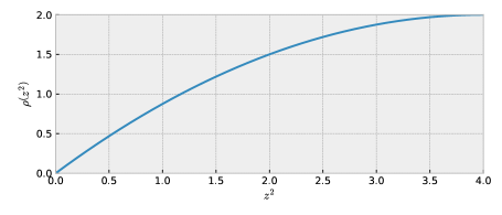
Figure 1: $\rho(z^{2})$ vs. $z^{2}$ curve that results from using a cosine distance-based attention.

And as a final point of comparison, thresholding attention weights between nodes that are sufficiently dissimilar has been proposed as a simple heuristic to increase robustness (Zhang and Zitnik, 2020; Wu et al., 2019b). This can also be incorporated with TWIRLS per the second row of Table 1, and hence be motivated within our integrated framework.

7.5 TWIRLS Relationship with Prior UGNN Models

While some previous UGNN models can be traced back to an underlying energy function and/or propagation layers related to gradient descent (Klicpera et al., 2019a; Ma et al., 2020; Pan et al., 2021; Zhang et al., 2020; Zhou et al., 2004; Zhu et al., 2021), TWIRLS is the only architecture we are aware of whereby all components, including propagation layers, nonlinear activations, and layer-wise adaptive attention all explicitly follow from iterations that provably descend a principled, possibly non-convex/non-smooth objective. In contrast, prior work has primarily relied on quadratic energy functions that produce identity activations, and if attention is considered at all, it is fixed to either a constant or a function of the input features $X$.

8 Experiments

In this section, we compare the performance of IGNN, the TWIRLS variant of UGNN we developed in Section 7, and the IGNN/UGNN hybrid EIGNN model. Under different application scenarios, we also evaluate against SOTA methods specifically designed for the particular task at hand.

For IGNN, we optionally set $W_{p}$ to either be $I$ or trainable parameters and report the best result among the two settings. For the attention used in TWIRLS, we select $\rho$ as a truncated $\ell_{p}$ quasinorm (Wilansky, 2013), and when no attention is included, we refer to the model as $\text{TWIRLS}_{\text{base}}$. For full details regarding the propagation steps, attention formulation, and other hyperparameters, please see the Appendix; similarly for experimental details, additional ablation studies and empirical results. All models and experiments were implemented using the Deep Graph Library (DGL) (Wang et al., 2019).

8.1 Base Model Results with No Attention

We first evaluate $\text{TWIRLS}_{\text{base}}$, EIGNN, and IGNN on three commonly used citation datasets, namely Cora, Pubmed and Citeseer (Sen et al., 2008), plus ogbn-arxiv (Hu et al., 2020), a relatively large dataset. For the citation datasets, we use the semi-supervised setting from (Yang et al., 2016), while for ogbn-arxiv, we use the standard split from the Open Graph Benchmark (OGB) leaderboard (see https://ogb.stanford.edu). We also compare $\text{TWIRLS}_{\text{base}}$, EIGNN, and IGNN against several top-performing baseline models, excluding those that rely on training heuristics such as adding labels as features, recycling label predictions, non-standard losses/optimization methods, etc. The latter, while practically useful, can be applied to all models to further boost performance and are beyond the scope of this work. Given these criteria, in Table 2 we report results for JKNet (Xu et al., 2018), GCNII (Chen et al., 2020), and DAGNN (Liu et al., 2020). Additionally, we include three common baseline models, GCN (Kipf and Welling, 2017), SGC (Wu et al., 2019a) and APPNP (Klicpera et al., 2019a). Overall, the $\text{TWIRLS}_{\text{base}}$ UGNN variant is particularly competitive.

We also conduct experiments showing the behavior of $\text{TWIRLS}_{\text{base}}$ as the number of propagation step becomes arbitrarily large. The results on Cora data are plotted in Figure 2, where we observe that the performance of $\text{TWIRLS}_{\text{base}}$ converges to the analytical solution given by

$$Y^{*}=\arg\min_{Y}\ell_{Y}\left(Y;W_{x},f\right)=(I+\lambda L)^{-1}f(X),$$ (34)

where $\ell_{Y}\left(Y;W_{x},f\right)$ is defined in (5), without performance degradation from oversmoothing. In contrast, the accuracy of SGC drops considerably with propagation.

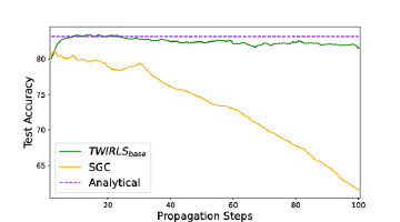
Figure 2: Accuracy versus propagation steps on Cora.

Model	Cora	Citeseer	Pubmed	Arxiv
SGC	81.7 ± 0.1	71.3 ± 0.2	78.9 ± 0.1	69.79 ± 0.16
GCN	81.5	71.1	79.0	71.74 ± 0.29
APPNP	83.3	71.8	80.1	71.74 ± 0.29
JKNet	81.1	69.8	78.1	72.19 ± 0.21
GCNII	85.5 ± 0.5	73.4 ± 0.6	80.3 ± 0.4	72.74 ± 0.16
DAGNN	84.4 ± 0.5	73.3 ± 0.6	80.5 ± 0.5	72.09 ± 0.25
IGNN	83.3 ± 0.7	71.2 ± 0.8	79.4 ± 0.6	71.1 ± 0.2
EIGNN	81.7 ± 0.9	70.9 ± 1.1	77.8 ± 0.4	-
$\text{TWIRLS}_{\text{base}}$	84.1 ± 0.5	74.2 ± 0.45	80.7 ± 0.5	72.93 ± 0.19

Table 2: Baseline results on standard benchmarks. Although EIGNN is highly memory efficient, the computational complexity is much higher than other models in certain cases (see Appendix for details), making application to larger benchmarks infeasible. Hence we do not show results on Arxiv, where hyperparameter tuning is prohibitively slow.

Dataset	Texas	Wisconsin	Actor	Cornell
Hom. Ratio (${\mathcal{H}}$)	0.11	0.21	0.22	0.3
GCN	59.46$\pm$5.25	59.80$\pm$6.99	30.26$\pm$0.79	57.03$\pm$4.67
GAT	58.38$\pm$4.45	55.29$\pm$8.71	26.28$\pm$1.73	58.92$\pm$3.32
GraphSAGE	82.43$\pm$6.14	81.18$\pm$5.56	34.23$\pm$0.99	75.95$\pm$5.01
Geom-GCN	67.57	64.12	31.63	60.81
$\text{H}_{2}\text{GCN}$	84.86$\pm$6.77	86.67$\pm$4.69	35.86$\pm$1.03	82.16$\pm$4.80
MLP	81.89$\pm$4.78	85.29$\pm$3.61	35.76$\pm$0.98	81.08$\pm$6.37
IGNN	83.1$\pm$5.6	79.2$\pm$6.0	35.5$\pm$2.9	76.0$\pm$6.2
EIGNN	80.54$\pm$5.67	83.72$\pm$3.46	34.74$\pm$1.19	81.08$\pm$5.70
$\text{TWIRLS}_{\text{base}}$	81.62$\pm$5.51	82.75$\pm$7.83	37.10$\pm$1.07	83.51$\pm$7.30
$\text{TWIRLS}_{\text{}}$	84.59$\pm$3.83	86.67$\pm$4.19	37.43$\pm$1.50	86.76$\pm$5.05

Table 3: Result on heterophily graphs.

8.2 Adversarial Attack Results

To showcase robustness against edge uncertainty using the proposed IRLS-based attention, we next test the full $\text{TWIRLS}_{\text{}}$ model using graph data attacked via the the Mettack algorithm (Zügner and Günnemann, 2019). Mettack operates by perturbing graph edges with the aim of maximally reducing the node classification accuracy of a surrogate GNN model that is amenable to adversarial attack optimization. And the design is such that this reduction is generally transferable to other GNN models trained with the same perturbed graph. In terms of experimental design, we follow the exact same non-targeted attack scenario from (Zhang and Zitnik, 2020), setting the edge perturbation rate to 20%, adopting the ‘Meta-Self’ training strategy, and a GCN as the surrogate model.

For baselines, we use three state-of-the-art defense models, namely GNNGuard (Zhang and Zitnik, 2020), GNN-Jaccard (Wu et al., 2019b) and GNN-SVD (Entezari et al., 2020). Results on Cora and Citeseer data are reported in Table 4, where the inclusion of attention provides a considerable boost in performance over $\text{TWIRLS}_{\text{base}}$ as well as EIGNN and IGNN alternatives. And somewhat surprisingly, $\text{TWIRLS}_{\text{}}$ generally performs comparably or better than existing SOTA models that were meticulously designed to defend against adversarial attacks.

Table 4: Adversarial attack comparison with SOTA models.

Model	ATK-Cora	ATK-Citeseer
surrogate (GCN)	57.38 ± 1.42	60.42 ± 1.48
GNNGuard	70.46 ± 1.03	65.20 ± 1.84
GNN-Jaccard	64.51 ± 1.35	63.38 ± 1.31
GNN-SVD	66.45 ± 0.76	65.34 ± 1.00
EIGNN	65.16 ± 0.78	68.36 ± 1.01
IGNN	61.47 ± 2.30	64.70 ± 1.26
$\text{TWIRLS}_{\text{base}}$	62.89 ± 1.59	63.83 ± 1.95
$\text{TWIRLS}_{\text{}}$	70.23 ± 1.09	70.63 ± 0.93

8.3 Results on Heterophily Graphs

We also consider non-homophily (or heterophily) graphs to further validate the effectiveness of our IRLS-based attention layers in dealing with inconsistent edges. In this regard, the homophily level of a graph can be quantified via the homophily ratio ${\mathcal{H}}=\frac{|\{(u,v)~{}:~{}(u,v)\in\mathcal{E}\land t_{u}=t_{v}\}|}{|\mathcal{E}|}$ from (Zhu et al., 2020b), where $t_{u}$ and $t_{v}$ are the target labels of nodes $u$ and $v$. ${\mathcal{H}}$ quantifies the tendency of nodes to be connected with other nodes from the same class. Graphs with an ${\mathcal{H}}\approx 1$ exhibit strong homophily, while conversely, those with ${\mathcal{H}}\approx 0$ show strong heterophily, indicating that many edges are connecting nodes with different labels.

We select four graph datasets with a low homophily ratio, namely, Actor, Cornell, Texas, and Wisconsin, adopting the data split, processed node features, and labels provided by (Pei et al., 2019). We compare the average node classification accuracy of our model with GCN (Kipf and Welling, 2017), GAT (Velickovic et al., 2018), GraphSAGE (Hamilton et al., 2017), SOTA heterophily methods GEOM-GCN (Pei et al., 2019) and $\text{H}_{2}\text{GCN}$ (Zhu et al., 2020b), as well as a baseline MLP as reported in (Zhu et al., 2020b).

Results are presented in Table 3, paired with the homophily ratios of each dataset. Here we observe that the proposed IRLS-based attention helps $\text{TWIRLS}_{\text{}}$ generally perform better than $\text{TWIRLS}_{\text{base}}$, EIGNN, IGNN, and other existing methods on heterophily graphs, achieving SOTA accuracy on three of the four datasets, and nearly so on the forth.

8.4 Results on Long-Dependency Data

Finally we test the ability of the models to capture long-range dependencies in graph data by stably introducing an arbitrary number of propagation layers without the risk of oversmoothing. For this purpose, we apply the Amazon Co-Purchase dataset, a common benchmark used for testing long-range dependencies given the sparse labels relative to graph size (Dai et al., 2018; Gu et al., 2020). We adopt the test setup from (Dai et al., 2018; Gu et al., 2020), and compare performance using different label ratios. We include five baselines, namely SGC (Chen et al., 2020), GCN (Kipf and Welling, 2017), GAT (Velickovic et al., 2018), SSE (Dai et al., 2018) and IGNN (Gu et al., 2020). Note that SSE and IGNN are explicitly designed for capturing long-range dependencies. Even so, our TWIRLS model is able to outperform both of them by a significant margin. The results are displayed in Figures 8.4 and 4.

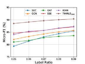
Figure 3: Amazon co-purchase results in Micro-F1.

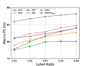
Figure 4: Amazon co-purchase results in Macro-F1.

8.5 Direct Comparison of UGNN and IGNN

As prior work has already showcased the value of IGNN and UGNN models across various graph prediction tasks, in this section we narrow our attention to complementary experiments designed to elucidate some of the particular issues raised by our analysis in previous sections. To this end, we begin by exploring the interplay between the type of graph propagation weights (symmetric vs asymmetric), the graph propagation path length (finite as with UGNN vs approximately infinite as with IGNN), and model expressiveness. For this purpose we design the following quasi-synthetic experiment: First, we train separate IGNN and UGNN models on the ogbn-arxiv dataset, where the architectures are equivalent with the exception of $W_{p}$ and the number of propagation steps (see Appendix for all network and training details). Additionally, because UGNN requires symmetric propagation weights, a matching parameter count can be achieved by simply expanding the UGNN hidden dimension. Once trained, we then generate predictions from each model and treat them as new, ground-truth labels. We next train four additional models separately on both sets of synthetic labels: (i) An IGNN with architecture equivalent to the original used for generating labels, (ii) an analogous UGNN, (iii) an IGNN with symmetric weights, and (iv) a UGNN with asymmetric weights (equivalent to IGNN with finite propagation steps). For all models the number of parameters is a small fraction of the number of labels to mitigate overfitting issues.

Results are presented in Table 5, where the columns indicate the label generating models, and the rows denote the recovery models. As expected, the highest recovery accuracy occurs when the generating and recovery models are matched such that perfect recovery is theoretically possible by design. We also observe that UGNN with asymmetric weights (denoted “UGNN/as”) performs significantly worse recovering IGNN data, indicating that truncated propagation steps can reduce performance when the true model involves long-range propagation. Similarly, IGNN with symmetric weights (IGNN/s) struggles somewhat to recover IGNN labels, indicating that symmetric weights may not always be able to exactly mimic asymmetric ones across all practical settings, which is not surprising. IGNN/s is however reasonably effective at recovering UGNN data given that the later involves symmetric weights and finite propagation steps. In general though, the fact that the performance of all models varies within a range of a few percentage points suggests a significant overlap of model expressiveness as might be expected.

8.6 Time and Memory Consumption

Next, in terms of time and memory consumption, we compare UGNN and IGNN on the Amazon Co-purchase benchmark, which has been advocated in (Gu et al., 2020) as a suitable data source for testing IGNN. Results are shown in Figures 5 and 6 based on executing 100 steps of training and evaluation on a single Tesla T4 GPU. Clearly, IGNN maintains a huge advantage in terms of memory consumption, while UGNN has a faster runtime provided the number of propagation steps is not too large. Further comparative analysis regarding the time complexity of UGNN and IGNN is provided in the Appendix.

	IGNN	UGNN
IGNN	95.7 ± 0.9	91.0 ± 1.5
UGNN	89.8 ± 1.9	94.5 ± 0.8
IGNN/s	90.2	93.2
UGNN/as	91.6 ± 1.2	92.3 ± 0.7

Table 5: Accuracy recovering synthetic labels

Figure 5: Memory cost

Figure 6: Running time

9 Conclusions

This work has closely examined the relationship between IGNNs and UGNNs, shedding light on their similarities and differences. In this regard, representative take-home messages are as follows:

• IGNN should in principle have an advantage when long-range propagation is required; however, standard node classification benchmarks are not generally adequate for fully showcasing this advantage (e.g., as evidenced by Table 2 results).

• UGNN symmetric propagation weights do not appear to be a significant hindrance, at least in terms of model expressiveness and subsequent node classification accuracy, while UGNN nonlinear propagation operators can be advantageous relative to IGNN when unreliable edges are present (e.g., as shown in comparisons involving the TWIRLS UGNN model applied to heterophily graphs or adversarial attacks).

• IGNN has a major advantage in memory costs, while UGNN sometimes has a practical advantage in complexity and accuracy (although with more refined future benchmarks the latter may not always be true).

• Both models benefit from the inductive biases of their respective design criteria, which occasionally overlap but retain important areas of distinction.

Note that in addition to the above, we have also derived TWIRLS, a simple UGNN variant that seamlessly combines propagation, nonlinear activations, and graph attention layers all anchored to the iterative descent of an objective function that is robust against edge uncertainty and oversmoothing. And despite its generic underpinnings, TWIRLS can match or exceed the performance of many existing architectures, including domain-specific SOTA models tailored to handle adversarial attacks, heterophily, or long-range dependencies.

Appendix A Datasets, Experiment Details and Model Specifications

In this section we introduce the detail of the experiments as well as give a detailed introduction of the architecture of UGNN used in this paper.

A.1 Datasets

Standard Benchmarks  In Section 8.1 of the main paper, we used four datasets, namely Cora, Citeseer, Pubmed and ogb-arxiv. These four are all citation datasets, i.e. their nodes represent papers and edges represents citation relationship. The node features of the former three are bag-of-words. Following (Yang et al., 2016), we use a fixed spitting for these three datasets in which there are 20 nodes per class for training, 500 nodes for validation and 1000 nodes for testing. For ogbn-arxiv, the features are word2vec vectors. We use the standard leaderboard splitting for ogbn-arxiv, i.e. papers published until 2017 for training, papers published in 2018 for validation, and papers published since 2019 for testing.

Adversarial Attack Experiments  As mentioned in the main paper, we tested on Cora and Citerseer using Mettack. We use the DeepRobust library (Li et al., 2020b) and apply the exact same non-targeted attack setting as in (Zhang and Zitnik, 2020). For all the baseline results in Table 4, we run the implementation in the DeepRobust library or the GNNGuard official code. Note the GCN-Jaccard results differ slightly from those reported in (Zhang and Zitnik, 2020), likely because of updates in the DeepRobust library and the fact that (Zhang and Zitnik, 2020) only report results from a single trial (as opposed to averaged results across multiple trails as we report).

Heterophily Experiments  In Section 8.3, we use four datasets introduced in (Pei et al., 2019), among which Cornell, Texas, and Wisconsin are web networks datasets, where nodes correspond to web pages and edges correspond to hyperlinks. The node features are the bag-of-words representation of web pages. In contrast, the Actor dataset is induced from a film-director-actor-writer network (Tang et al., 2009), where nodes represent actors and edges denote co-occurrences on the same Wikipedia page. The node features represent some keywords in the Wikipedia pages. We used the data split, processed node features, and labels provided by (Pei et al., 2019), where for the former, the nodes of each class are randomly split into 60%, 20%, and 20% for train, dev and test set respectively.

Long-Range Dependency/Sparse Label Tests  In Section 8.4, we adopt the Amazon Co-Purchase dataset, which has previously been used in (Gu et al., 2020) and (Dai et al., 2018) for evaluating performance involving long-range dependencies. We use the dataset provided by the IGNN repo (Gu et al., 2020), including the data-processing and evaluation code, in order to obtain a fair comparison. As for splitting, 10% of nodes are selected as the test set. And because there is no dev set, we directly report the test result of the last epoch. We also vary the fraction of training nodes from 5% to 9%. Additionally, because there are no node features, we learn a 128-dim feature vector for each node. All of these settings from above follow from (Gu et al., 2020).

Summary Statistics  Table 6 summarizes the attributes of each dataset.

Table 6: Dataset statistics. The FEATURES column describes the dimensionality of node features. Note that the Amazon Co-Purchase dataset has no node features.

Dataset	Nodes	Edges	Features	Classes
Cora	2,708	5,429	1,433	7
Citeseer	3,327	4,732	3,703	6
Pubmed	19,717	44,339	500	3
Arxiv	169,343	1,166,243	128	40
Texas	183	309	1,703	5
Wisconsin	251	499	1,703	5
Actor	7,600	33,544	931	5
Cornell	183	295	1,703	5
Amazon	334,863	2,186,607	-	58

A.2 Experiment Details

In all experiments of IGNN and EIGNN, we optionally set $W_{p}^{s}$ to be trainable parameters or fix it to $I$. For IGNN, following the original paper, we optionally set $f(X)=\mathrm{MLP}(PX)$ or $\mathrm{MLP}(X)$, while for EIGNN and TWIRLS we only set $f(X)=\mathrm{MLP}(X)$.

In label recovering task in Section 8.5 and the evaluation of time and memory in Section 8.6, for the purpose of comparing finite vs infinite number of propagations and symmetric vs asymmetric weights, we ignore irrelevant options such as different choice of $f(X)$, hidden size, and the attention mechanism in UGNN. We always use $f(X)=XW_{x}$ and $g\left[\mbox{\boldmath$y$}_{i}^{*}(\mathcal{W});\theta\right]=W_{g}\mbox{\boldmath$y$}_{i}^{*}(\mathcal{W})$ where $W_{g}\in\mathbb{R}^{c\times d}$ is a learned matrix that maps the propagated node features to the output space. We set the hidden size to $32$ in asymmetric case and $34$ in symmetric case to ensure nearly the same number of parameters (we deliberately set the hidden size to this small to ensure the models do not overfit). For generating models, we first train them using the original labels of the dataset by 500 steps. For UGNN, we fix the number of propagation steps is set to $2$, and adopt (11) of UGNN.

When projecting $W_{p}$ (or $\tilde{W}$ in UGNN) to the space that admits unique fixed point, in IGNN’s original paper it uses $\|\cdot\|_{\mathrm{inf}}$ (Gu et al., 2020), which would break the symmetry, based on our result in Section 5.1, in our implementation when the model weight is symmetric we project $\|\cdot\|_{2}$ instead of $\|\cdot\|_{\mathrm{inf}}$. In EIGNN, we use rescaling as in (Liu et al., 2021a) instead of projection.

In the direct comparison between IGNN and UGNN in Section 8.5 and the time $\&$ memory comparison in Section 8.6, we always use normalized adjacency $P=\hat{A}$ for propagation matrix. However, in other experiments with TWIRLS, we allow extra flexibility of the propagation matrix of TWIRLS.

A.3 Basic UGNN Architecture

The UGNN architecture is composed of the input module $f\left(X;W\right)$, followed by the unfolded propagation layers defined by (8), concluding with $g(\mbox{\boldmath$y$};\theta)$.

For TWIRLS, which has an attention mechanism, the aggregate design is depicted in in Figure 7. For simplicity, we generally adopt a single attention layer sandwiched between equal numbers of propagation layers; however, for heterophily datasets we apply an extra attention layer before propagation. Note that the attention only involves reweighting the edge weights of the graph (i.e., it does not alter the node embeddings at each layer).

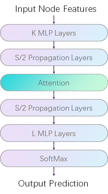
Figure 7: Model Architecture. $S$ is the total number of propagation steps. $K$ and $L$ are number of MLP layers before and after the propagation respectively. While not a requirement, in all of our experiments, either $K$ or $L$ is set to zero, meaning that the MLP exists on only one side of the propagation layers.

A.4 TWIRLS Model Variations

Pre-conditioning and Reparameterization   If we unfold the iteration step of (5), define the reparameterized embeddings $Z=\tilde{D}^{1/2}Y$ and left multiply the update rule by $\tilde{D}^{1/2}$, we have

$$Z^{(k+1)} =(1-\alpha)Z^{(k)}+\alpha\lambda\tilde{D}^{-1/2}AY^{(k)}+\alpha\tilde{D}^{-1/2}f(X;W)$$

$$=(1-\alpha)Z^{(k)}+\alpha\lambda\tilde{D}^{-1/2}A\tilde{D}^{-1/2}Z^{(k)}+\alpha\tilde{D}^{-1}Z^{(0)}.$$ (35)

From here, if we choose $\alpha=\lambda=1$, for $Z^{(1)}$ we have that

$$Z^{(1)} = \left(\tilde{D}^{-1/2}A\tilde{D}^{-1/2}+\tilde{D}^{-1}\right)Z^{(0)}$$ (36)

$$= \tilde{D}^{-1/2}\tilde{A}\tilde{D}^{-1/2}Z^{(0)},$$

which gives the exact single-layer GCN formulation in $Z$-space with $Z^{(0)}=f(X;W)$.

Normalized Laplacian Unfolding  From another perspective, if we replace $L$ in (5) with a normalized graph Laplacian, and then take gradients steps as before, there is no need to do preconditioning and reparameterizing. For example, unfolding (5) with $L$ changed to the symmetrically-normalized version $\tilde{L}=I-\tilde{D}^{-1/2}\tilde{A}\tilde{D}^{-1/2}$, we get

$$Y^{(k+1)}=(1-\alpha-\alpha\lambda)Y^{(k)}+\alpha\lambda\tilde{D}^{-1/2}\tilde{A}\tilde{D}^{-1/2}Y^{(k)}+\alpha Y^{(0)},$$ (37)

where we set $\tilde{D}=I+D$. This formula is essentially the same as (35). The main difference is that there is no $\tilde{D}^{-1}$ in front of $X$, which indicates an emphasis on the initial features. We found this version to be helpful on ogbn-arxiv and Amazon Co-Purchase data. Note however that all of our theoretical support from the main paper applies equally well to this normalized version, just with a redefinition of the gradient steps to include the normalized Laplacian.

A.5 Specific Attention Formula

While the proposed attention mechanism can in principle adopt any concave, non-decreasing function $\rho$, in this work we restrict $\rho$ to a single functional form that is sufficiently flexible to effectively accommodate all experimental scenarios. Specifically, we adopt

$$\rho(z^{2})=\begin{cases}\bar{\tau}^{p-2}z^{2}&\quad\text{if }z<\bar{\tau}\\ \tfrac{2}{p}\bar{T}^{p}-\rho_{0}&\quad\text{if }z>\bar{T}\\ \tfrac{2}{p}z^{p}-\rho_{0}&\quad\text{otherwise},\end{cases}$$ (38)

where $p$, $\bar{T}$, and $\bar{\tau}$ are non-negative hyperparameters and $\rho_{0}=\frac{2-p}{p}\bar{\tau}^{p}$ is a constant that ensures $\rho$ is continuous. Additionally, the gradient of $\rho$ produces the attention score function (akin to $\gamma$ in the main paper) given by

$$s(z^{2})\triangleq\frac{\partial p(z^{2})}{\partial z^{2}}=\begin{cases}\bar{\tau}^{p-2}&\quad\text{if }z<\bar{\tau}\\ 0&\quad\text{if }z>\bar{T}\\ z^{p-2}&\quad\text{otherwise}.\end{cases}$$ (39)

And for convenience and visualization, we also adopt the reparameterizations $\tau=\bar{\tau}^{\frac{1}{2-p}}$ and $T=\bar{T}^{\frac{1}{2-p}}$, and plot $\rho(z^{2})$ and $s(z^{2})$ in Figure 8 using $p=0.1$, $\tau=0.2$, $T=2$.

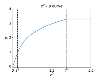
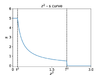
Figure 8: A visualization of attention functions.

Overall, this flexible choice has a natural interpretation in terms of its differing behavior between the intervals $[0,\bar{\tau}]$, $(\bar{\tau},\bar{T})$, and $(\bar{T},\infty)$. For example, in the $[0,\bar{\tau}]$ interval a quadratic penalty is applied, which leads to constant attention independent of $z$. This is exactly like $\text{TWIRLS}_{\text{base}}$. In contrast, within the $(\bar{T},\infty)$ interval $\rho$ is constant and the corresponding attention weight is set to zero (truncation), which is tantamount to edge removal. And finally, the middle interval provides a natural transition between these two extremes, with $\rho$ becoming increasingly flat with larger $z$ values.

Additionally, many familiar special cases emerge for certain parameter selections. For example $T=\infty$ corresponds with no explicit truncation, while $p=2$ can instantiate no attention. And $T=\tau$ means we simply truncate those edges with large distance, effectively keeping the remaining edge attention weights at $1$ (note that there is normalization during propagation, so setting edges to a constant is equivalent to setting them to $1$).

Appendix B Furthur Model Analysis

In this section we provide some extended analysis, including the time complexity as well as how EIGNN may be derived from the UGNN framework.

B.1 Time Complexity

The time complexity of UGNN is $O(mdS+Nd^{2})$, where $m$ is the number of edges, $S$ is the number of propagation steps, $N$ and $d$ are the number of MLP layers and hidden size respectively. By contrast, the time complexity of a GCN is $O(mdN+Nd^{2})$. Moreover, if the MLP layers are all after propagation (i.e., no parameters before propagation), the time complexity can be reduced to $O(Nd^{2})$ by precomputing the propagation (i.e., the same as an MLP).

For IGNN, the time consumption depends on the number of iteration steps to find the fixed point, which relates to certain properties of weight matrix $W_{p}$. However, in implementation in the official IGNN code the authors propagate a certain number of steps or until an acceptable error rate is obtained. If the number of iteration steps is $T$, then the time complexity is $O(mdT+Nd^{2})$, which is essentially the same as UGNN (and other message passing-based GNNs) but replace $S$ with $T$, the number of iteration steps to find the fixed point.

For EIGNN, based on its linearity, the overall propagation matrix can be pre-computed in $O(N^{3})$ time. Note that after pre-computing the overall propagation matrix, it does not need to be re-computed during training, which saves the time complexity to $O(Nd^{2})$ in training. However, in practice, when the size of graph is very large, even $O(N^{3})$ pre-computing is a huge overhead, not to mention it needs to be recomputed every time when propagation-related hyper-parameters change.

B.2 EIGNN as a Special Case of UGNN

As claimed in the main paper, the EIGNN model can be viewed as a special case of UGNN; we provide the details here. We begin with the general energy from (3), and then choose $\phi\left(\mbox{\boldmath$y$};W_{\phi}\right)=0$, $\rho\left(z^{2}\right)=z^{2}$, and adopt the weight parameterization $W_{P}^{s}=s^{2}F^{\top}F$, where $F$ is a trainable parameter matrix and $s$ is a rescaling factor given by

$$s=\left(\|F^{\top}F\|_{\mathcal{+}}\epsilon_{F}\right)^{-\frac{1}{2}}\text{.}$$ (40)

This produces the simplified loss

$$\ell_{Y}(Y;W_{x},f)=\|Y-f(X;W_{x})\|_{\mathcal{F}}^{2}+\mu\mathrm{tr}\left[F^{\top}Y^{\top}LYF\right]\text{,}$$ (41)

where $P=I-L$ is the normalized adjacency matrix. A gradient step on (41) initialized at $Y^{(k)}$ can then be computed as

$$Y^{(k+1)}=\gamma s^{2}F^{\top}FY^{(k)}W_{p}^{s}+f\left(X,W_{x}\right),$$ (42)

which matches the original EIGNN updates from (Liu et al., 2021a).

Appendix C Notation Used in Proofs

In following sections, we give proofs of all propositions in the main paper. We first introduce some notations used in proofs here.

For simplicity, in following sections we denote $\ell_{Y}(Y;{\mathcal{W}},f,\rho,\widetilde{B},\phi)$ in (3) by $\ell_{Y}(Y)$, denote $\phi\left(\mbox{\boldmath$y$}_{i};W_{\phi}\right)$ by $\phi(\mbox{\boldmath$y$}_{i})$ and $\sum_{i}\phi(\mbox{\boldmath$y$}_{i})$ by $\phi(Y)$, and denote $f(X;W)$ by $f(X)$. And the smooth part of $\ell_{Y}$ is denoted by $\ell_{Y}^{s}(Y)=\ell_{Y}(Y)-\phi(Y)$. And we possibly ignore the parameter of the function (e.g. $\ell_{Y}$).

We denote the vectorization of a matrix $M$ by $\mathrm{vec}(M)$ and the Kronecker product of two matrices $M_{1}$ and $M_{2}$ denoted by $M_{1}\otimes M_{2}$.

For Fréchet subdifferential respect to $Y$, we denote it by $\partial_{Y}$, ignoring the subscript _F used in main paper.

Appendix D Proofs Related to UGNN Convergence

In this section, we investigate different conditions to guarantee convergence (to stationary point) of UGNN under different assumptions of $\ell_{Y}$.

To start with, we first prove that as long as proximal gradient descent has a fixed point, the fixed point is a stationary point.

Lemma 15.

For any $Z$ such that

$$Z\in\arg\min_{Y}\frac{1}{2\alpha}\left\|Y-\left(Z-\alpha\nabla\ell_{Y}^{s}(Z)\right)\right\|_{\mathcal{F}}^{2}+\phi(Y)$$ (43)

it must hold that $0\in\partial_{Z}\ell_{Y}(Z)$.

Proof  We will use the summation property and local minimality property of Fréchet subdifferential (see (Li et al., 2020a) for detailed descriptions). For any $Y^{\prime}$ such that

$$Y^{\prime}\in\arg\min_{Y}\frac{1}{2\alpha}\left\|Y-\left(Z-\alpha\nabla\ell_{Y}^{s}(Z)\right)\right\|_{\mathcal{F}}^{2}+\phi(Y),$$ (44)

we have

$$0\in\partial_{Y}\left.\left[\frac{1}{2\alpha}\left\|Y-\left(Z-\alpha\nabla\ell_{Y}^{s}(Z)\right)\right\|_{\mathcal{F}}^{2}+\phi(Y)\right]\right|_{Y=Y^{\prime}}.$$ (45)

It follows that

$$0\in\nabla\ell_{Y}^{s}(Z)+\partial_{Y^{\prime}}\phi(Y^{\prime}).$$ (46)

So, if $Y^{\prime}=Z$, we have

$$0\in\nabla\ell_{Y}^{s}(Z)+\partial_{Z}\phi(Z)=\partial_{Z}\left[\ell_{Y}^{s}(Z)+\phi(Z)\right]=\partial_{Z}\ell_{Y}(Z)$$ (47)

With Lemma 15, to prove that UGNN converges to a stationary point, we only need to show it has a fixed point.

For the convergence of UGNN, we assume $\phi$ is continuous and $\ell_{Y}$ is Lipschitz smooth (i.e. its gradient is Lipschitz continuous) with Lipschitz constant $\mathcal{L}$. And we further distinguish two cases 1) No other conditions provided 2) $\phi$ is convex and $\ell_{Y}$ is strongly convex. We will use different strategies to prove convergence and show that the conditions on the step-size that guarantee convergence are different in these two cases.

Note that, as mentioned in the main paper, in the first case, we also need to assume $\ell_{Y}(Y)\to\infty$ when $\|Y\|\to\infty$ to avoid a degenerate case that the process goes to infinite.

The Framework of Proving Convergence

To prove the convergence of the iteration of (8), we will use Zangwill’s convergence theorem. For clarity, we state it next.

Proposition 16 (Zangwill’s Convergence Theorem (Luenberger, 1984)).

Let $A:\mathcal{X}\to 2^{\mathcal{X}}$ be a set-valued function, $\mathcal{G}\subset\mathcal{X}$ be a solution set (which can be any set we are interested in). For any sequence $\{\mbox{\boldmath$x$}_{k}\}_{k=1}^{\infty}$ such that $\mbox{\boldmath$x$}_{k+1}\in A(\mbox{\boldmath$x$}_{k})$, if the following conditions hold jointly:

1. (boundedness) $\{\mbox{\boldmath$x$}_{k}|1\leq k\leq\infty\}$ is contained in some compact subset of $\mathcal{X}$.

2. (descent function) there exists a continuous function $\ell$ such that

   1. if $\mbox{\boldmath$x$}\not\in\mathcal{G}$, then $\forall\mbox{\boldmath$y$}\in A(\mbox{\boldmath$x$}),\ell(\mbox{\boldmath$y$})<\ell(\mbox{\boldmath$x$})$.

   2. if $\mbox{\boldmath$x$}\in\mathcal{G}$, then $\forall\mbox{\boldmath$y$}\in A(\mbox{\boldmath$x$}),\ell(\mbox{\boldmath$y$})\leq\ell(\mbox{\boldmath$x$})$.

3. (closedness) the mapping $A$ is closed at all point of $\mathcal{X}\setminus\mathcal{G}$ i.e. $\{(\mbox{\boldmath$x$},\mbox{\boldmath$y$})|\mbox{\boldmath$x$}\in\mathrm{clos}\left(\mathcal{X}\setminus\mathcal{G}\right),\mbox{\boldmath$y$}\in A(\mbox{\boldmath$x$})\}$ is a closed set, where $\mathrm{clos}$ means set closure.

then the limit of any convergent subsequence of $\{\mbox{\boldmath$x$}_{k}\}_{k=1}^{\infty}$ is a solution i.e. inside $\mathcal{G}$.

Given Lemma 15, we define the solution set $\mathcal{G}$ as set of fixed points:

$$\mathcal{G}=\left\{Z\left|Z\in\arg\min_{Y}\frac{1}{2\alpha}\left\|Y-\left(Z-\alpha\nabla\ell_{Y}^{s}(Z)\right)\right\|_{\mathcal{F}}^{2}+\phi(Y)\right.\right\}.$$ (48)

Then the proof is composed of three steps:

1. showing there exists some function that is a descent function;

2. showing the process is closed;

3. showing $\left\{Y^{(k)}\right\}_{k=1}^{\infty}$ are bounded.

Thereinto, the closedness is a straightforward consequence of Lemma 6 in (Sriperumbudur and Lanckriet, 2009). For boundedness, as long as we find some descent function $\ell$, we consider the set $\mathcal{S}=\left\{Y~{}|~{}\ell(Y)\leq\ell\left(Y^{(0)}\right)\right\}$. Apparently $\left\{Y^{(k)}\right\}_{k=1}^{\infty}\subseteq\mathcal{S}$, so we only need to show that $\mathcal{S}$ is bounded. It suffices to prove $\displaystyle\lim_{\|Y\|\to\infty}\ell(Y)=\infty$. Therefore, step 2 is already finished and step 3 is nearly finished. The most tricky part is proving descent of some function.

D.1 UGNN Convergence in General Case

Here we don’t cast convexity assumption on the objective function. In this case we choose $\ell_{Y}$ as the candidate descent function. Note that by the assumption that $\displaystyle\lim_{\|Y\|\to\infty}\ell_{Y}(Y)=\infty$ made in main paper, we have boundedness of $\mathcal{S}$.

To prove descent, we first prove loosely descent (i.e. Lemma 1) and then show when $Y^{(k)}\not\in\mathcal{G}$, it is also strict.

Proof of Lemma 1    Here we first state a property of Lipschitz smooth function:

Proposition 17 ((Bertsekas, 1999)).

for any $\ell(\mbox{\boldmath$y$})$ whose gradient is $\mathcal{L}$-Lipschitz, it satisfies

$$\forall\mbox{\boldmath$y$},\mbox{\boldmath$z$},\ell(\mbox{\boldmath$y$})\leq\ell(\mbox{\boldmath$z$})+\nabla\ell(\mbox{\boldmath$z$})^{\top}(\mbox{\boldmath$y$}-\mbox{\boldmath$z$})+\frac{\mathcal{L}}{2}\|\mbox{\boldmath$y$}-\mbox{\boldmath$z$}\|_{2}^{2}.$$ (49)

From Proposition 17, if function $\ell$ is $\mathcal{L}$-Lipschitz smooth, then for any $\mbox{\boldmath$z$},\mbox{\boldmath$y$}$, we have

$$\ell(\mbox{\boldmath$y$}) \leq\ell(\mbox{\boldmath$z$})+\nabla\ell(\mbox{\boldmath$z$})^{\top}(\mbox{\boldmath$y$}-\mbox{\boldmath$z$})+\frac{\mathcal{L}}{2}\|\mbox{\boldmath$y$}-\mbox{\boldmath$z$}\|_{2}^{2}$$ (50)

$$=\ell(\mbox{\boldmath$z$})+\nabla\ell(\mbox{\boldmath$z$})^{\top}\mbox{\boldmath$y$}-\nabla\ell(\mbox{\boldmath$z$})^{\top}\mbox{\boldmath$z$}+\frac{\mathcal{L}}{2}\|\mbox{\boldmath$y$}\|_{2}^{2}+\frac{\mathcal{L}}{2}\|\mbox{\boldmath$z$}\|_{2}^{2}-\mathcal{L}\mbox{\boldmath$y$}^{\top}\mbox{\boldmath$z$}$$ (51)

$$=\ell(\mbox{\boldmath$z$})-\frac{1}{2\mathcal{L}}\|\nabla\ell(\mbox{\boldmath$z$})\|_{2}^{2}$$

$$~{}~{}+\frac{\mathcal{L}}{2}\left[\frac{1}{\mathcal{L}^{2}}\|\nabla\ell(\mbox{\boldmath$z$})\|_{2}^{2}+\|\mbox{\boldmath$y$}\|_{2}^{2}+\|\mbox{\boldmath$z$}\|_{2}^{2}+\frac{2}{\mathcal{L}}\nabla\ell(\mbox{\boldmath$z$})^{\top}\mbox{\boldmath$y$}-\frac{2}{\mathcal{L}}\nabla\ell(\mbox{\boldmath$z$})^{\top}\mbox{\boldmath$z$}-2\mbox{\boldmath$y$}^{\top}\mbox{\boldmath$z$}\right]$$ (52)

$$=\ell(\mbox{\boldmath$z$})-\frac{1}{2\mathcal{L}}\|\nabla\ell(\mbox{\boldmath$z$})\|_{2}^{2}+\frac{\mathcal{L}}{2}\left\|\mbox{\boldmath$y$}-\left[\mbox{\boldmath$z$}-\frac{1}{\mathcal{L}}\nabla\ell(\mbox{\boldmath$z$})\right]\right\|_{2}^{2}.$$ (53)

Taking $\ell(\mbox{\boldmath$y$})=\ell_{Y}^{s}(\mbox{\boldmath$y$})$, $\mbox{\boldmath$y$}=\mathrm{vec}(Y)$ and $\mbox{\boldmath$z$}=\mathrm{vec}\left(Y^{(k)}\right)$, and let

$$\beta_{Y}\left(Y^{(k)}\right)=\ell_{Y}^{s}\left(Y^{(k)}\right)-\frac{\alpha}{2}\left\|\nabla\ell_{Y}^{s}\left(Y^{(k)}\right)\right\|_{\mathcal{F}}^{2},$$ (54)

we can define an upper-bound of $\ell_{Y}$:

$$\ell_{Y}^{(\mathrm{upp})}(Y;Y^{(k)}) =\frac{1}{2\alpha}\left\|Y-\left[Y^{(k)}-\alpha\nabla\ell\left(Y^{(k)}\right)\right]\right\|_{\mathcal{F}}^{2}+\sum_{i}\phi(\mbox{\boldmath$y$}_{i})+\beta_{Y}\left(Y^{(k)}\right)$$ (55)

$$=\frac{1}{2\alpha}\left\|Y-U^{(k)}\right\|_{\mathcal{F}}^{2}+\sum_{i}\phi(\mbox{\boldmath$y$}_{i})+\beta_{Y}\left(Y^{(k)}\right),$$ (56)

and adopting (53) we have that:

$$\ell_{Y}(Y)=\ell_{Y}^{s}(Y)+\sum_{i}\phi(\mbox{\boldmath$y$}_{i})\leq\ell_{Y}^{(\mathrm{upp})}.$$ (57)

(Notice that since we have assumed $\alpha\leq\frac{1}{\mathcal{L}}$, $\ell_{Y}$ is also $\frac{1}{\alpha}$-Lipschitz). It’s not difficult to check $\ell_{Y}^{(\mathrm{upp})}\left(Y^{(k)};Y^{(k)}\right)=\ell_{Y}\left(Y^{(k)}\right)$. Also, since adding terms which is not related to $Y$ does not affect the $\arg\min$ result in (8), we have that

$$Y^{(k+1)} \in\arg\min_{Y}\frac{1}{2\alpha}\|Y-U^{(k)}\|_{\mathcal{F}}^{2}+\sum_{i}\phi(\mbox{\boldmath$y$}_{i})$$ (58)

$$=\arg\min_{Y}\frac{1}{2\alpha}\|Y-U^{(k)}\|_{\mathcal{F}}^{2}+\sum_{i}\phi(\mbox{\boldmath$y$}_{i})+\beta_{Y}\left(Y^{(k)}\right)$$ (59)

$$=\arg\min_{Y}\ell_{Y}^{(\mathrm{upp})}\left(Y;Y^{(k)}\right).$$ (60)

Then we have

$$\ell_{Y}\left(Y^{(k+1)}\right)\leq\ell_{Y}^{(\mathrm{upp})}\left(Y^{(k+1)};Y^{(k)}\right)\leq\ell_{Y}^{(\mathrm{upp})}\left(Y^{(k)};Y^{(k)}\right)=\ell_{Y}\left(Y^{(k)}\right),$$ (61)

which proves the the lemma.

Furthermore, when $Y^{(k)}\not\in\mathcal{G}$, i.e.$Y^{(k)}\not\in\arg\min\ell_{Y}^{(\mathrm{upp})}\left(Y;Y^{(k)}\right)$, we have that

$$\ell_{Y}^{(\mathrm{upp})}\left(Y^{(k+1)};Y^{(k)}\right)<\ell_{Y}^{(\mathrm{upp})}\left(Y^{(k)};Y^{(k)}\right),$$ (62)

and thus (61) holds strictly, which matches the condition of strictly descent given in Proposition 16.

D.2 UGNN Convergence Under Convexity

When $\ell_{Y}^{s}$ is strongly convex and $\phi$ is convex, we have already know the existence and uniqueness of stationary point (global optimum) $Y^{*}$, so by Lemma 15 the fixed point of iteration (8) must be $Y^{*}$, i.e. $\mathcal{G}=\{Y^{*}\}$. In this case, we choose the distance of current point to the fixed point $\ell(Y)=\left\|Y-Y^{*}\right\|_{\mathcal{F}}^{2}$ as the descent function. As long as descent is proved, the boundedness of $\ell(Y)$ is obvious.

We prove the descent of $\ell(Y)$ by using the fact that when $\phi$ and $\ell_{Y}^{s}$ are convex, the proximal operator $\mathrm{prox}_{\phi}$ is non-expansive and the gradient step is contraction with small enough $\alpha$.

For proximal operator, Proposition 1 in (Gribonval and Nikolova, 2020) has already shown that as long as $\phi$ is convex, $\mathrm{prox}_{\phi}$ is non-expansive, i.e.

$$\forall\mbox{\boldmath$x$},\mbox{\boldmath$y$},\left\|\mathrm{prox}_{\phi}(\mbox{\boldmath$x$})-\mathrm{prox}_{\phi}(\mbox{\boldmath$y$})\right\|_{2}\leq\|\mbox{\boldmath$x$}-\mbox{\boldmath$y$}\|_{2}.$$ (63)

Thus we only need to prove gradient descent is contraction. To prove this, we first introduce another property of convex Lipschitz smooth function:

Proposition 18 (Theorem 2.1.5 of (Nesterov, 2003)).

For any function $\ell$ that is convex and whose gradient is $\mathcal{L}$-Lipschitz continuous, we have

$$\forall\mbox{\boldmath$x$},\mbox{\boldmath$y$},\left[\nabla\ell(\mbox{\boldmath$x$})-\nabla\ell(\mbox{\boldmath$y$})\right]^{\top}(\mbox{\boldmath$x$}-\mbox{\boldmath$y$})\geq\frac{1}{\mathcal{L}}\|\nabla\ell(\mbox{\boldmath$x$})-\nabla\ell(\mbox{\boldmath$y$})\|_{2}^{2}.$$ (64)

Then we prove the contraction of gradient descent:

Lemma 19.

for any function $\ell$ that is $\mathcal{L}$-Lipschitz smooth satisfies that

$$\forall\mbox{\boldmath$x$},\mbox{\boldmath$y$},\left\|\left[\mbox{\boldmath$x$}-\alpha\nabla\ell(\mbox{\boldmath$x$})\right]-\left[\mbox{\boldmath$y$}-\alpha\nabla\ell(\mbox{\boldmath$y$})\right]\right\|_{2}^{2}\leq(1-\alpha^{2}\mathcal{L}^{2}-2\alpha\mathcal{L})\|\mbox{\boldmath$x$}-\mbox{\boldmath$y$}\|_{2}^{2}.$$ (65)

Proof  From Proposition 18, we have that:

$$\left\|\left[\mbox{\boldmath$x$}-\alpha\nabla\ell(\mbox{\boldmath$x$})\right]-\left[\mbox{\boldmath$y$}-\alpha\nabla\ell(\mbox{\boldmath$y$})\right]\right\|_{2}^{2}$$ (66)

$$= \|\mbox{\boldmath$x$}-\mbox{\boldmath$y$}\|_{2}^{2}+\alpha^{2}\|\nabla\ell(\mbox{\boldmath$x$})-\nabla\ell(\mbox{\boldmath$y$})\|_{2}^{2}-2\alpha(\mbox{\boldmath$x$}-\mbox{\boldmath$y$})^{\top}\left[\nabla\ell(\mbox{\boldmath$x$})-\nabla\ell(\mbox{\boldmath$y$})\right]$$ (67)

$$\leq \|\mbox{\boldmath$x$}-\mbox{\boldmath$y$}\|_{2}^{2}+\left(\alpha^{2}-\frac{2\alpha}{\mathcal{L}}\right)\left\|\nabla\ell(\mbox{\boldmath$x$})-\nabla\ell(\mbox{\boldmath$y$})\right\|_{2}^{2}$$ (68)

$$\leq (1-\alpha^{2}\mathcal{L}^{2}-2\alpha\mathcal{L})\|\mbox{\boldmath$x$}-\mbox{\boldmath$y$}\|_{2}^{2},$$ (69)

which finishes the proof.

Combining (63) and Lemma 19, we get following corollary:

Corollary 20.

For $\ell_{Y}(Y)=\ell_{Y}^{s}(Y)+\phi(Y)$, where $\ell_{Y}^{s}$ is strongly convex and $\mathcal{L}$-Lipschitz smooth, $\phi$ is convex, $\alpha<\frac{2}{\mathcal{L}}$, we have

$$\left\|Y^{(k+1)}-Y^{*}\right\|_{\mathcal{F}}<\left\|Y^{(k)}-Y^{*}\right\|_{\mathcal{F}}$$ (70)

if $Y^{(k)}\neq Y^{*}$.

Proof  Since $Y^{*}$ is the fixed point, we have $Y^{*}\in\mathrm{prox}_{\phi}\left[Y^{*}-\alpha\nabla\ell_{Y}^{s}(Y^{*})\right]$, therefore by (63)

$$\left\|Y^{(k+1)}-Y^{*}\right\|_{\mathcal{F}} =\left\|\mathrm{prox}_{\phi}\left[Y^{(k)}-\alpha\nabla\ell_{Y}^{s}\left(Y^{(k)}\right)\right]-\mathrm{prox}_{\phi}\left[Y^{*}-\alpha\nabla\ell_{Y}^{s}(Y^{*})\right]\right\|_{\mathcal{F}}^{2}$$ (71)

$$\leq\left\|\left[Y^{(k)}-\alpha\nabla\ell_{Y}^{s}\left(Y^{(k)}\right)\right]-\left[Y^{*}-\alpha\nabla\ell_{Y}^{s}(Y^{*})\right]\right\|_{\mathcal{F}}^{2}$$ (72)

Since $\alpha<\frac{2}{\mathcal{L}}$, from Lemma 19 we have that when $Y^{(k)}\neq Y^{*}$,

$$\left\|\left[Y^{(k)}-\alpha\nabla\ell_{Y}^{s}\left(Y^{(k)}\right)\right]-\left[Y^{*}-\alpha\nabla\ell_{Y}^{s}(Y^{*})\right]\right\|_{\mathcal{F}}^{2}<\left\|Y^{(k)}-Y^{*}\right\|.$$ (73)

Therefore, $\ell\left(Y^{(k)}\right)=\left\|Y^{(k)}-Y^{*}\right\|$ is strictly descent when $Y^{(k)}\neq Y^{*}$. Combining this and Proposition 16 we conclude that:

Theorem 21.

When $\ell_{Y}^{s}(Y)$ is $\mathcal{L}$-Lipschitz smooth and strongly convex, $\phi(Y)$ is continuous and convex, iteration (8) converges to the unique global minimum of $\ell_{Y}$ when $\alpha<\frac{2}{\mathcal{L}}$.

D.3 Remarks

Note that, the upper-bound of $\alpha$ is different in the two cases. Actually, if there is no penalty term $\phi$, i.e. no proximal step, in both cases the upper bound is $2/\mathcal{L}$, which is a standard result on gradient descent for smooth functions that can be found in any optimization textbook. To get some intuition, considering the upper bound derived in (56), although $\alpha=1/\mathcal{L}$ is the optimal step size to minimize $\ell^{(\mathrm{upp})}_{Y}$, with $\alpha$ relaxed to $\leq 2/\mathcal{L}$, $\ell^{(\mathrm{upp})}_{Y}$ still goes down:

$$\ell_{Y}^{(\mathrm{upp})}\left[Y^{(k)}-\alpha\nabla\ell_{Y}^{s}\left(Y^{(k)}\right);Y^{(k)}\right]\leq\ell_{Y}^{(\mathrm{upp})}\left(Y^{(k)};Y^{(k)}\right)=\ell_{Y}^{s}\left(Y^{(k)}\right).$$ (74)

However, this is no longer true when the proximal step is added. Thus in the latter case, we either cast a more strict bound on $\alpha$ to still guarantee descent of $\ell_{Y}$, or add extra assumptions that the process is non-expansive to guarantee that the output of each iteration would not be pushed further away from the fixed point despite not ensuring the descent of $\ell_{Y}$.

D.4 Other Related Proofs

Note that Lemma 1 and Theorem 7 has been proved in section D.1 . Here we provide other missing proofs from Section 5.1.

Proof of Theorem 3  First, we will show that $\ell_{Y}^{s}$ is strongly convex under conditions given. We have

$$\mathrm{vec}\left(\frac{\partial\ell_{Y}^{s}}{\partial Y}\right) =\mathrm{vec}\left[YW_{f}^{s}-f(X;W)+\tilde{L}YW_{p}^{s}\right]$$ (75)

$$=\left(W_{f}^{s}\otimes I+W_{p}^{s}\otimes\tilde{L}\right)\mathrm{vec}(Y)+\mathrm{vec}\left[f(X;W)\right]$$ (76)

$$=\Sigma\mathrm{vec}(Y)+\mathrm{vec}\left[f(X;W)\right].$$ (77)

Therefore the Hessian of $\ell_{Y}^{s}$ is

$$\frac{\partial^{2}\ell_{Y}^{s}}{\partial\mathrm{vec}(Y)^{2}}=\Sigma.$$ (78)

We also know that when $\lambda_{\tiny\mbox{min}}(\Sigma)>0$, $\ell_{Y}^{s}$ is strongly convex respect to $Y$, thus has a unique global minimum. And from Proposition 1 in (Gribonval and Nikolova, 2020), we know $\phi$ is convex through the non-expansiveness of $\sigma$.

Furthermore, the $\lambda_{\tiny\mbox{max}}(\Sigma)$ is the Lipschitz constant of $\ell^{s}_{Y}$, and from theorem 21 we know when $\alpha<2/\lambda_{\tiny\mbox{max}}(\Sigma)$ the algorithm converges to the stationary point, which is the global optimum.

Proof of Corollary 4    Taking $W_{f}^{s}=I-W_{p}^{s}$ and $P=I-\tilde{L}$, we have that

$$\Sigma=I-P\otimes W_{p}^{s}.$$ (79)

By the spectral properties of Kronecker product, we have

$$\lambda_{\tiny\mbox{min}}(\Sigma)\geq 1-\left\|W_{p}^{s}\right\|_{2}\left\|P\right\|_{2}>0$$ (80)

and

$$\lambda_{\tiny\mbox{max}}(\Sigma)\leq 1+\left\|W_{p}^{s}\right\|_{2}\left\|P\right\|_{2}<2.$$ (81)

The discussion in Section 4.3 mentioned that to get (11), we need to set $\alpha=1<\frac{2}{\lambda_{\tiny\mbox{max}}(\Sigma)}$, therefore from Theorem 3 we conclude that (11) converges to the global minimum of (12).

Proof of Lemma 5 (Convergence of IGNN)  We first convert (2) to the vector form:

$$\mathrm{vec}\left(Y^{(k+1)}\right)=\sigma\left[\left(W_{p}\otimes P\right)\mathrm{vec}\left(Y^{(k)}\right)+\mathrm{vec}(f)\right],$$ (82)

where $f=f(X;W_{x})$, ignoring the parameters for simplicity. Let $M=W_{p}\otimes P$. From the spectral properties of knronecker product, we have

$$\|M\|_{2}=\|W_{p}\|_{2}\|P\|_{2}<1.$$ (83)

By definition of matrix norm we have

$$\forall\mbox{\boldmath$x$}_{1},\mbox{\boldmath$x$}_{2},\|M(\mbox{\boldmath$x$}_{1}-\mbox{\boldmath$x$}_{2})\|_{2}\leq\|M\|_{2}\|\mbox{\boldmath$x$}_{1}-\mbox{\boldmath$x$}_{2}\|_{2},$$ (84)

which means $M$ (as a linear transformation) is a contraction mapping on Euclidean space. We also assumed $\sigma$ is contraction mapping, and thus from Banach’s fixed point theorem(Kinderlehrer and Stampacchia, 1980) we conclude that (82), as well as (2), has a unique fixed point.

Appendix E Proofs Related to The Expressiveness

In this section, we provide detailed proofs of propositions in Section 6, as well as an analysis under cases where activation functions are non-linear.

E.1 Proof of Lemma 2

This lemma is a straight-forward corollary of Theorem 1 in (Gribonval and Nikolova, 2020). For clarity, we excerpt the theorem here:

Proposition 22 (Theorem 1 in (Gribonval and Nikolova, 2020)).

Let $\mathcal{H}$ be some Hilbert space (e.g. $\mathbb{R}^{k}$) and $\mathcal{Y}\subset\mathcal{H}$ be non-empty. A function $\sigma:\mathcal{Y}\to\mathcal{H}$ is the proximal operator of a function $\phi:\mathcal{H}\to\mathbb{R}\cup\{+\infty\}$ if and only if there exists a convex l.s.c. (lower semi-continuous) function $\psi:\mathcal{H}\to\mathbb{R}\cup\{+\infty\}$ such that for each $\mbox{\boldmath$y$}\in\mathcal{Y},\sigma(\mbox{\boldmath$y$})\in\partial\psi(\mbox{\boldmath$y$})$.

Since our $\sigma$ is component-wise, we only need to consider $\mathcal{Y}=\mathcal{H}=\mathbb{R}$. Furthermore, since $\sigma(\mbox{\boldmath$x$})$ is continuous, its indefinite integration exists. Let $\psi(\mbox{\boldmath$x$})=\int\sigma(\mbox{\boldmath$x$})\mathrm{d}\mbox{\boldmath$x$}$, which must be convex since its derivative is non-decreasing. Then according to Proposition 22, there exists a function $\phi$ whose proximal operator is $\sigma$. Conversely, if there exists $\phi$ such that $\sigma=\mathrm{prox}_{\phi}$, from Proposition 22 it is the subdifferential of some convex function $\psi$, which means it is non-decreasing.

E.2 Proof of Lemma 6

We only need a counterexample to prove this. Suppose $n=1$ and $d=2$, consider $W=\begin{bmatrix}0&1\\ 0&0\end{bmatrix}$, $Y=\begin{bmatrix}a&b\end{bmatrix}$, then $YW=\begin{bmatrix}0\\ a\end{bmatrix}$.

If there exists any second order smooth function $h$ such that $\frac{\partial h}{\partial a}=0$ and $\frac{\partial h}{\partial b}=a$, we have that

$$\frac{\partial^{2}h}{\partial a\partial b}=0\neq\frac{\partial^{2}h}{\partial b\partial a}=1,$$

which contradicts the second order smoothness assumption of $h$.

E.3 Proof of Theorem 9

First consider a case which allows $T$ and $W_{p}^{s}$ to have complex values. Hereinafter we denote the space of all complex-valued matrices with shape $d_{1}\times d_{2}$ by $\mathbb{C}^{d_{1}\times d_{2}}$.

We recall Jordan’s decomposition theorem below. Let $J(\lambda)$ be Jordan block matrix

$$J(\lambda)=\begin{bmatrix}\lambda&1&&&\\ &\lambda&1&&\\ &&\lambda&&\\ &&&\ddots&1\\ &&&&\lambda\end{bmatrix}.$$

We have the following well-known fact.

Proposition 23 (Jordan).

For every $W\in\mathbb{R}^{d\times d}$, there exists a complex-valued invertible matrix $P\in\mathbb{C}^{d\times d}$ and complex-valued block-diagonal matrix

$$\Omega=\begin{bmatrix}J(\lambda_{1})&&&\\ &J(\lambda_{2})&&\\ &&\ddots&\\ &&&J(\lambda_{k})\end{bmatrix}$$

such that $W=P\Omega P^{-1}$, where $\lambda_{j}\in\mathbb{C}$ is the $j$-th eigenvalue of $W$ and the size of $J(\lambda_{j})$ is the algebraic multiplicity of $\lambda_{j}$.

Corollary 24.

If a square matrix $W\in\mathbb{R}^{d\times d}$ has $d$ distinct eigenvalues, then there exists $P,\Lambda\in\mathbb{C}^{d\times d}$ where $P$ is invertible and $\Lambda$ is diagonal, such that $W=P\Lambda P^{-1}$.

Then, we shall show that actually on the complex domain “almost” every matrix can be diagonalized, which means, for each matrix $W$, either it itself can be diagonalized, or there’s a diagonalizable matrix $W^{\prime}$ that is arbitrarily closed to $W$.

Corollary 25.

For every square matrix $W\in\mathbb{R}^{d\times d}$ and any $\epsilon>0$, there exists a diagonalizable square matrix $W^{\prime}\in\mathbb{R}^{d\times d}$ such that $\|W^{\prime}-W\|\leq\epsilon$.

Proof  Let $W=R\Omega R^{-1}$ and $E=\mathrm{diag}\begin{bmatrix}\epsilon_{1},&\epsilon_{2},&\cdots,&\epsilon_{n}\end{bmatrix}$ such that the diagonal of $\Omega+E$ is distinct and $\epsilon_{j}^{2}<\frac{\epsilon^{2}}{d\|R\|^{2}\|R^{-1}\|^{2}}$.

Since $\Omega$ is upper-triangle, its eigenvalues are the elements in its diagonal, which are distinct. Thus according to Corollary 24, $\Omega+E$ is diagonalizable, suppose $\Omega+E=Q\Lambda Q^{-1}$. Let $W^{\prime}=R(\Omega+E)R^{-1}=RQ\Lambda Q^{-1}R^{-1}$, it is apparent $W^{\prime}$ also diagonalizable.

Now consider the difference between $W^{\prime}$ and $W$. We have $\|W^{\prime}-W\|^{2}=\|PEP^{-1}\|^{2}\leq\|E\|^{2}\|R\|^{2}\|R^{-1}\|^{2}<\epsilon^{2}$.

Note the norm in Corollary 25 can be any matrix norm.

Lemma 26.

The solution to the equation $PYW+XW_{x}=Y$ is continuous respect to $W$ as long as a unique solution exists.

Proof  The solution of this equation is $\mathrm{vec}(Y)=\left(I-W^{\top}\otimes P\right)^{-1}\mathrm{vec}(XW_{x})$, which is continuous.

Theorem 27.

For any $W_{p}\in\mathbb{R}^{d\times d}$ that admits a unique fixed point for IGNN and $W_{x}\in\mathbb{R}^{d_{0}\times d}$, suppose $Y\in\mathbb{R}^{n\times d}$ is the only solution of $PYW+XW_{x}=Y$, then there exists a $Y^{\prime}\in\mathbb{C}^{n\times d},\bar{W}_{x}\in\mathbb{C}^{d_{0}\times d^{\prime}}$, right-invertible $\bar{T}\in\mathbb{C}^{d\times d^{\prime}}$ and herimitian $\bar{W}_{p}^{s}\in\mathbb{C}^{d^{\prime}\times d^{\prime}}$, such that

$$PY^{\prime}\bar{T}\bar{W}_{p}^{s}+X\bar{W}_{x}=Y^{\prime}\bar{T},\text{ with }\|Y^{\prime}-Y\|<\epsilon,\forall\epsilon>0,Y^{\prime}\in\mathbb{C}^{n\times d}.$$ (85)

Proof  By Corollary 25 and Lemma 26, there exists diagonalizable $W^{\prime}\in\mathbb{R}^{d\times d}$ such that $PY^{\prime}W^{\prime}+XW_{x}=Y^{\prime}$ for some $Y^{\prime}$ satisfies $\|Y^{\prime}-Y\|<\epsilon$.

Suppose now $W^{\prime}=R\Lambda R^{-1}$ where $\Lambda$ is diagonal and $R$ is invertible. We have

$$PY^{\prime}R\Lambda R^{-1}+XW_{x}=Y^{\prime},$$ (86)

and right-multiply by $R$ at each side of this equation we get

$$P(Y^{\prime}R)\Lambda+XW_{x}R=Y^{\prime}R.$$ (87)

By choosing $\bar{T}=R,\bar{W}_{p}^{s}=\Lambda,\bar{W}_{x}=W_{x}R^{-1}$, we proved the theorem.

Next, we consider restricting this result to the real domain. This is straight-forward since every complex linear transformation can be converted to real linear transformation by consider real and imaginary parts separately. Hereinafter, we denote the real part of an complex-valued matrix $M$ by $M_{(r)}$ and imaginary part by $M_{(i)}$.

Proof of Theorem 9  Let $\bar{Y}$, $\bar{T}$, $\bar{W}_{p}^{s}$, $\bar{W}_{x}$ be the matrices obtained from Theorem 27. Note the last three are complex-valued, $\bar{T}$ is invertible and $\bar{W}_{p}^{s}$ is hermitian.

Consider $T=\begin{bmatrix}\bar{T}_{(r)}&\bar{T}_{(i)}\end{bmatrix}$. Since $\bar{T}$ is invertible, let $\bar{\text{\rotatebox{180.0}{$T$}}}=\bar{T}^{-1}$, then we have $I=(\bar{T}\bar{\text{\rotatebox{180.0}{$T$}}})_{(r)}=\bar{T}_{(r)}\bar{\text{\rotatebox{180.0}{$T$}}}_{(r)}-\bar{T}_{(i)}\bar{\text{\rotatebox{180.0}{$T$}}}_{(i)}$. Thus $T\begin{bmatrix}\bar{\text{\rotatebox{180.0}{$T$}}}_{(r)}\\ -\bar{\text{\rotatebox{180.0}{$T$}}}_{(i)}\end{bmatrix}=\bar{T}_{(r)}\bar{\text{\rotatebox{180.0}{$T$}}}_{(r)}-\bar{T}_{(i)}\bar{\text{\rotatebox{180.0}{$T$}}}_{(i)}=I$. This means $T$ is right-invertible.

Then let $W_{s}^{p}=\begin{bmatrix}\bar{W}^{s}_{p(r)}&\bar{W}^{s}_{p(i)}\\ -\bar{W}^{s}_{p(i)}&\bar{W}^{s}_{p(r)}\end{bmatrix}$. Since $\bar{W}^{s}_{p}$ is hermitian, we have that $\bar{W}^{s}_{p(r)}=\bar{W}^{s\top}_{p(r)}$ and $\bar{W}^{s}_{p(i)}=-\bar{W}^{s\top}_{p(i)}$, which ensures $W^{s}_{p}$ constructed here is symmetric. Finally, let $\tilde{W}_{x}=\begin{bmatrix}\bar{W}_{x(r)}&\bar{W}_{x(i)}\end{bmatrix}$. Now it’s easy to verify that $PY^{\prime}TW_{p}^{s}+X\tilde{W}_{x}=Y^{\prime}T$.

E.4 Proof of Theorem 10

First we will illustrate that by setting the parameters in UGNN to properly, the iteration step from (8) is equivalent to a GCN layer with symmetric shared weights, with or without residual connections. We set $\rho$ to be identity (so that $\Gamma=I$), $\tilde{B}$ satisfies that $\tilde{B}^{\top}\tilde{B}=I-P$ (e.g. if $P=\hat{A}=\tilde{D}^{-1/2}\tilde{A}\tilde{D}^{-1/2}$ is normalized adjacency, then $\tilde{B}$ is normalized incidence matrix $\tilde{B}=\tilde{D}^{-1/2}B$).

For a GCN model without residual connections, let $W_{f}^{s}=I-W_{p}^{s}$, then we have $Y^{(k+1)}=\sigma(PY^{(k)}W_{p}^{s})$. Consider $Y^{(0)}=W\begin{bmatrix}Y^{(0)}_{\mathrm{GCN}}&0&0&\cdots&0\end{bmatrix}$ where $Y^{(0)}_{\mathrm{GCN}}$ is the input of GCN, and the $i$th $0$ here denote a block matrix of all zero with the same size as $Y^{(i)}_{\mathrm{GCN}}$. When we let

$$W_{p}^{s}=\begin{bmatrix}&W_{p}^{(1)}&&&&\\ W_{p}^{(1)\top}&&W_{p}^{(2)}&&&\\ &W_{p}^{(2)\top}&&W_{p}^{(3)}&&\\ &&W_{p}^{(3)\top}&&\ddots&\\ &&&\ddots&&W_{p}^{(k)}\\ &&&&W_{p}^{(k)\top}&\end{bmatrix},$$ (88)

it is not difficult to verify that the $k$th block of $Y^{(k)}$ is $Y^{(k)}_{\mathrm{GCN}}$. Note the $0$s in the (88) are block matrices of all zeros with proper size.

For GCN model with residual connection, let $W_{f}^{s}=I-W_{p}^{s}-W_{r}^{s}$, then $Y^{(k+1)}=\sigma(PY^{(k)}W_{p}^{s}+Y^{(k)}W_{r}^{s})$. We take the same $W_{p}^{s}$ as before (88), and let

$$W_{r}^{s}=\begin{bmatrix}&I&&&&\\ I&&I&&&\\ &I&&I&&\\ &&I&&\ddots&\\ &&&\ddots&&I\\ &&&&I&\end{bmatrix}.$$ (89)

Since $W_{r}^{s}$ and $W_{p}^{s}$ are both symmetric, apparently $W_{f}^{s}$ is also symmetric. Also notice that since residual connection exists, the size of all the $W_{p}^{(i)}$s are the same, so the size of $I$ in the (89) is the same as $W_{p}^{(i)}$.

E.5 A Sufficient Condition of Equivalence of Symmetric and Asymmetric Weights

In this section, we give a sufficient condition of fixed-point equivalence of symmetric and asymmetric weights in general case as mentioned in Section 6.1. Here we consider general nonlinear functions $\sigma$ and penalty term $\phi$. Hereinafter we denote $\mathrm{prox}_{\phi}$ by $\tilde{\sigma}$.

Constraint on $\sigma$  To simplify the discussion, we add a mild assumption on $\sigma$ and consider a general type of $\tilde{\sigma}$: We assume $\sigma(\mbox{\boldmath$x$})$ is a proximal operator of some penalty function which is differentiable with respect to $x$.

This assumption is consistent with practice. Firstly, commonly used non-linearities like $\mathrm{tanh}$, $\mathrm{sigmoid}$ and ReLU are all proximal operators since they are all continuous and component-wise non-decreasing (By Lemma 2). Also, although at some point ReLU and Leaky-ReLU are not differentiable, we can approximate them by

$$\text{ReLU}(x)\approx\frac{1}{r}\log\left(\exp(rx)+1\right)$$

and

$$\text{Leaky-ReLU}(x,p)\approx\frac{1}{r}\log\left(\exp(rx)+\exp(prx)\right)$$

with big enough $r$, which are differentiable and do not affect their practical attributes.

$\tilde{\sigma}$ Considered  As discussed in the main paper, it would cause some degenerated cases if we allow a general class of proximal operators. Also it would too difficult to handle in this case. Therefore, we only consider proximal operators in a special while general family

$$\mathcal{S}=\{\tilde{\sigma}:\mbox{\boldmath$x$}\mapsto G\sigma(C\mbox{\boldmath$x$})|G,C\text{ are chosen such that }\tilde{\sigma}\text{ is proximal operator}\}$$

Now we consider under what value of $G$ and $C$ we can ensure $\tilde{\sigma}$ is proximal operator. From Proposition 22, we know $\exists\phi,\tilde{\sigma}=\mathrm{prox}_{\phi}$ iff $\tilde{\sigma}$ is subgradient of some l.s.c convex function. Since we have assumed $\sigma$ is continuous and differentiable, $\int\sigma(\mbox{\boldmath$x$})\mathrm{d}\mbox{\boldmath$x$}$ is twice differentiable. We know that a twice-differentiable function $\psi$ is convex iff its Hessian $H_{\psi}$ is positive semi-definite. Therefore the Hessian of $\sigma$ must be positive semi-definite, we denote it by $H(\mbox{\boldmath$x$})=\frac{\partial\sigma(\mbox{\boldmath$x$})}{\partial\mbox{\boldmath$x$}}$, and so do Hessian of $\tilde{\sigma}(\mbox{\boldmath$x$})$, which we denote by $\tilde{H}(\mbox{\boldmath$x$})=\frac{\partial\tilde{\sigma}(\mbox{\boldmath$x$})}{\partial\mbox{\boldmath$x$}}$. From the chain rule we have

$$\tilde{H}(\mbox{\boldmath$x$})=\frac{\partial\tilde{\sigma}(\mbox{\boldmath$x$})}{\partial\mbox{\boldmath$x$}}=\frac{\partial G\sigma(C\mbox{\boldmath$x$})}{\partial\mbox{\boldmath$x$}}=G\frac{\partial\sigma(C\mbox{\boldmath$x$})}{\partial C\mbox{\boldmath$x$}}\frac{\partial C\mbox{\boldmath$x$}}{\partial\mbox{\boldmath$x$}}=GH(C\mbox{\boldmath$x$})C.$$

From the deduction above, we can conclude that:

Lemma 28.

$\tilde{\sigma}:\mathbb{R}^{d}\to\mathbb{R}^{d},\mbox{\boldmath$x$}\mapsto G\sigma(C\mbox{\boldmath$x$})$ is proximal operator iff $\forall\mbox{\boldmath$x$}\in C\mathbb{R}^{d},GH(\mbox{\boldmath$x$})C$ is positive semi-definite where $H(\mbox{\boldmath$x$})=\frac{\partial\sigma(\mbox{\boldmath$x$})}{\partial\mbox{\boldmath$x$}}$.

The Condition of General Fixed-Point Alignment

Theorem 29.

For $\sigma$ satisfying the assumptions above, $W_{p}\in\mathbb{R}^{d\times d}$ that admits unique fixed point for IGNN, and $W_{x}\in\mathbb{R}^{d_{0}\times d}$, suppose $Y$ is the only solution of $Y=\sigma(PYW+XW_{x})$, a sufficient condition of

$$\exists\phi,\text{ right invertible }T\in\mathbb{R}^{d\times d^{\prime}},\text{ symmetric }W_{p}^{s}\in\mathbb{R}^{d^{\prime}\times d^{\prime}}\text{ and }\tilde{W}_{x}\in\mathbb{R}^{d\times d}\text{ such that }$$

$$\tilde{\sigma}(PYTW_{p}^{s}+XW_{x})=YT$$

is that

$$\exists\text{ right-invertible }T\in\mathbb{R}^{d\times d^{\prime}},C\in\mathbb{R}^{d^{\prime}\times d},W_{p}^{s}\in\mathbb{R}^{d^{\prime}\times d^{\prime}}\text{ such that }TW_{p}^{s}C=W_{p}$$

$$\text{ and }\forall\mbox{\boldmath$x$}\in C^{\top}\mathbb{R},T^{\top}H(\mbox{\boldmath$x$})C^{\top}\text{ is P.S.D,}$$

where $\tilde{\sigma}(\mbox{\boldmath$x$})=\mathrm{prox}_{\phi}(\mbox{\boldmath$x$})$ and $H(\mbox{\boldmath$x$})=\frac{\partial\sigma(\mbox{\boldmath$x$})}{\partial\mbox{\boldmath$x$}}$.

Proof  We have assumed $\tilde{\sigma}\in\mathcal{S}$, thus $\tilde{\sigma}(\mbox{\boldmath$x$})=G\sigma(C\mbox{\boldmath$x$})$. We want to prove that

$$YT =\tilde{\sigma}(PYTW_{p}^{s}+X\tilde{W}_{x})$$ (90)

$$=\sigma(PYTW_{p}^{s}C+X\tilde{W}_{x}C)G$$ (91)

$$=\sigma(PYTW_{p}^{s}C+XW_{x})G\text{ (Assume $\tilde{W}_{x}C=W_{x}$)}.$$ (92)

A sufficient condition for this equation to hold is $T=G$ and $Y=\sigma(AYTW_{p}^{s}C+XW_{x})=\sigma(AYW_{p}+XW_{x})$. Comparing the last two terms, apparently it holds when $TW_{p}^{s}C=W_{p}$. And to ensure $\tilde{\sigma}\in\mathcal{S}$, from Lemma 28 we know it means $T^{\top}H(C^{\top}x)C^{\top}$ be positive semi-definite for all $x$.

We can verify this Theorem 29 by linear case. If $\sigma$ is linear, then $H(Cx)=I$, thus simply taking $C=T^{-1}$ (on complex field) we have $TW_{p}^{s}T^{-1}$ can generate any real matrix $W$ and $T^{\top}H(C^{\top}x)C^{\top}=T^{\top}T^{-\top}=I$ is positive semi-definite.

Appendix F Proofs Related to The Robust UGNN Regularization

This section provide detailed proofs of all propasitions in Section 7.

F.1 Proof of Lemma 11

A function $f:\mathbb{R}_{+}\rightarrow\mathbb{R}_{+}$ is said to be totally monotone (Widder, 2015) if it is continuous on $[0,\infty)$ and infinitely differentiable on $(0,\infty)$, while also satisfying

$$(-1)^{n}\frac{\partial^{n}}{\partial u^{n}}f(z)~{}\geq~{}0,~{}~{}\forall~{}n=1,2,\ldots.$$ (93)

for all $z>0$. Furthermore, a non-negative symmetric function $p_{z}(z)$ can be expressed as a Gaussian scale mixture, i.e.,

$$p_{z}\left(z\right)=\int{\mathcal{N}}\left(z|0,\gamma^{-1}I\right)d\mu\left(\gamma\right),$$ (94)

for some positive measure $\mu$, iff $p_{z}(\sqrt{z})$ is a totally monotone function on $[0,\infty)$ (Andrews and Mallows, 1974). However, as shown in (Palmer et al., 2006), any such totally monotone function can be expressed as $p_{z}(\sqrt{z})=\exp\left[-\rho(z)\right]$, where $\rho$ is a concave, non-decreasing function. From these results, and the assignment $z_{ij}=\sqrt{\mbox{\boldmath$u$}_{ij}^{\top}\mbox{\boldmath$u$}_{ij}}=\|\mbox{\boldmath$y$}_{i}-\mbox{\boldmath$y$}_{j}\|_{2}$, we can then infer that

$$-\log p(Y)$$ (95)

$$\equiv-\sum_{\{i,j\}\in{\mathcal{E}}}\log\int{\mathcal{N}}\left(\mbox{\boldmath$u$}_{ij}|0,\gamma^{-1}_{ij}I\right)d\mu\left(\gamma_{ij}\right)$$

$$=-\sum_{\{i,j\}\in{\mathcal{E}}}\log\int\left(\tfrac{\gamma_{ij}}{2\pi}\right)^{d/2}\exp\left[-\tfrac{\gamma_{ij}}{2}\mbox{\boldmath$u$}^{\top}_{ij}\mbox{\boldmath$u$}_{ij}\right]d\mu\left(\gamma_{ij}\right)$$

$$=-\sum_{\{i,j\}\in{\mathcal{E}}}\log\int\left(\tfrac{\gamma_{ij}}{2\pi}\right)^{1/2}\exp\left[-\tfrac{\gamma_{ij}}{2}z_{ij}^{2}\right]d\mu^{\prime}\left(\gamma_{ij}\right)$$

$$=-\sum_{\{i,j\}\in{\mathcal{E}}}\log\int{\mathcal{N}}\left(z_{ij}|0,\gamma^{-1}_{ij}I\right)d\mu^{\prime}\left(\gamma_{ij}\right)$$

$$=-\sum_{\{i,j\}\in{\mathcal{E}}}\log p_{z}\left(z_{ij}\right)$$

$$=-\sum_{\{i,j\}\in{\mathcal{E}}}\log p_{z}\left(\sqrt{\|\mbox{\boldmath$y$}_{i}-\mbox{\boldmath$y$}_{j}\|^{2}_{2}}\right)$$

$$=\sum_{\{i,j\}\in{\mathcal{E}}}\rho\left(\|\mbox{\boldmath$y$}_{i}-\mbox{\boldmath$y$}_{j}\|^{2}_{2}\right),$$

where the positive measure $\mu^{\prime}$ is defined such that $d\mu^{\prime}(\gamma_{ij})=\left(\tfrac{\gamma_{ij}}{2\pi}\right)^{(d-1)/2}d\mu(\gamma_{ij})$, noting that prior results apply equally well to this updated version for some concave non-decreasing $\rho$. Hence Lemma 11 directly follows.

F.2 Proof of Lemma 12 and Corollary 13

Both Lemma 12 and Corollary 13 follow directly from principles of convex analysis and Fenchel duality (Rockafellar, 1970). In particular, any concave, non-decreasing function $\rho:\mathbb{R}_{+}\rightarrow\mathbb{R}$ can be expressed via the variational decomposition

$$\rho\left(z^{2}\right) = \min_{\gamma>0}\left[\gamma z^{2}-\rho^{*}\left(\gamma\right)\right]$$ (96)

$$\geq \gamma z^{2}-\widetilde{\rho}\left(\gamma\right),$$

where $\gamma$ is a variational parameter whose optimization defines the decomposition, and $\widetilde{\rho}$ is the concave conjugate of $\rho$. From a visual perspective, (96) can be viewed as constructing $\rho\left(z^{2}\right)$ as the minimal envelope of a series of quadratic upper bounds, each defined by a different value of $\gamma$. And for any fixed $\gamma$, we obtain a fixed upper bound once we remove the minimization operator. By adopting $z=\|\mbox{\boldmath$y$}_{i}-\mbox{\boldmath$y$}_{j}\|_{2}$ for all $i,j\in{\mathcal{E}}$ we obtain (7.2), which by construction satisfies (22). And (12) follows by noting that at any optimal $\gamma^{*}$, the upper bound satisfies

$$\gamma^{*}z^{2}-\widetilde{\rho}\left(\gamma^{*}\right)=\rho\left(z^{2}\right),$$ (97)

i.e., it is tangent to $\rho$ at $z^{2}$, in which case $\gamma^{*}$ must be equal to the stated gradient (or subgradient).

And finally, in terms of Corollary 13, let $Y^{*}=\arg\min_{Y}\ell_{Y}(Y;\rho)$. We may then simply apply Lemma 12 to form the bound

$$\hat{\ell}_{Y}(Y^{*};\Gamma,\widetilde{\rho})~{}~{}\geq~{}~{}\hat{\ell}_{Y}(Y^{*};\Gamma^{*},\widetilde{\rho})~{}~{}=~{}~{}\ell_{y}(Y^{*};\rho),$$ (98)

where $\Gamma^{*}$ denotes a diagonal matrix with optimized $\gamma_{ij}^{*}$ values along the diagonal. Therefore $\hat{\ell}_{Y}(Y;\Gamma^{*},\widetilde{\rho})$ so-defined achieves the stated result.

F.3 Proof of Lemma 14

Based on Lemma 12 and (12), as well as the analogous update rule for $\Gamma^{(k+1)}$ from (7), it follows that

$$\hat{\ell}_{Y}\left(Y^{(k)};\Gamma^{(k+1)},\widetilde{\rho}\right)~{}~{}=~{}~{}\ell_{Y}(Y^{(k)};\rho).$$ (99)

Now define $\Psi(Y)\triangleq\hat{\ell}_{Y}\left(Y;\Gamma^{(k+1)},\widetilde{\rho}\right)$ and

$$\hat{\Psi}(Y) \triangleq \Psi\left(Y^{(k)}\right)+$$

$$\nabla\Psi\left(Y^{(k)}\right)^{\top}\left(Y-Y^{(k)}\right)+\tfrac{{\mathcal{L}}}{2}\left\|Y-Y^{(k)}\right\|_{{\mathcal{F}}}^{2},$$

where $\Psi$ has Lipschitz continuous gradients with Lipschitz constant ${\mathcal{L}}$ satisfying

$$\left\|\nabla\Psi(Y_{1})-\nabla\Psi(Y_{2})\right\|_{{\mathcal{F}}}\leq{\mathcal{L}}\left\|\Psi(Y_{1})-\Psi(Y_{2})\right\|_{{\mathcal{F}}}$$ (101)

for all $Y_{1}$ and $Y_{2}$. We may then conclude that

$$\hat{\Psi}(Y)~{}~{}\geq~{}~{}\Psi(Y)~{}~{}\geq~{}~{}\ell_{Y}(Y;\rho),$$ (102)

with equality at the point $Y=Y^{(k)}$. Note that the first inequality in the above expression follows from basic results in convex analysis (e.g., see Bubeck (2014)[Lemma 3.4]), while the second comes from (22). Consequently, by adopting $Y^{(k+1)}=Y^{(k)}-\alpha\nabla\Psi Y^{(k)}$, which is equivalent to (28), we have that

$$\hat{\Psi}\left(Y^{(k+1)}\right) =\hat{\Psi}\left(Y^{(k)}-\alpha\nabla\Psi Y^{(k)}\right)$$ (103)

$$=\Psi\left(Y^{(k)}\right)+\left(\frac{\mathcal{L}\alpha^{2}}{2}-\alpha\right)\left\|\nabla\Psi\left(Y^{(k)}\right)\right\|$$ (104)

$$\leq\Psi\left(Y^{(k)}\right)$$ (105)

Note the inequality from (104) to (105) holds as long as we adopt a step-size $\alpha\leq\tfrac{2}{{\mathcal{L}}}$. Hence we must only enforce the Lipschitz constraint (101) to guarantee monotonicity. This is equivalent to the requirement that ${\mathcal{L}}I-\nabla^{2}\Psi\left(Y^{(k)}\right)\succeq 0$ for all $k$, which computes to ${\mathcal{L}}I\succeq 2\left(I+\lambda B^{\top}\Gamma^{(k)}B\right)$. Setting ${\mathcal{L}}$ to be greater than or equal to the maximum singular value of $2\left(I+\lambda B^{\top}\Gamma^{(k)}B\right)$ satisfies this objective, which then leads to the step-size bound $\alpha\leq\left\|\lambda B^{\top}\Gamma^{(k)}B+I\right\|_{2}^{-1}$.

References

- Andrews and Mallows (1974) David Andrews and Colin Mallows. Scale mixtures of normal distributions. J. Royal Statistical Society: Series B, 36(1), 1974.
- Bai et al. (2019) Shaojie Bai, J Zico Kolter, and Vladlen Koltun. Deep equilibrium models. arXiv preprint arXiv:1909.01377, 2019.
- Bertsekas (1999) Dimitri Bertsekas. Nonlinear Programming. Athena Scientific, 2nd edition, 1999.
- Bubeck (2014) Sébastien Bubeck. Convex optimization: Algorithms and complexity. Foundations and Trends in Machine Learning, 2014.
- Chartrand and Yin (2008) Rick Chartrand and Wotao Yin. Iteratively reweighted algorithms for compressive sensing. International Conference on Accoustics, Speech, and Signal Processing, 2008.
- Chen et al. (2018) Jie Chen, Tengfei Ma, and Cao Xiao. FastGCN: Fast learning with graph convolutional networks via importance sampling. International Conference on Learning Representations, 2018.
- Chen et al. (2020) Ming Chen, Zhewei Wei, Zengfeng Huang, Bolin Ding, and Yaliang Li. Simple and deep graph convolutional networks. In Proceedings of the 37th International Conference on Machine Learning, ICML, volume 119, pages 1725–1735, 2020.
- Chen and Eldar (2021) Siheng Chen and Yonina C Eldar. Graph signal denoising via unrolling networks. In ICASSP 2021-2021 IEEE International Conference on Acoustics, Speech and Signal Processing (ICASSP), pages 5290–5294, 2021.
- Chen et al. (2017) Yichen Chen, Dongdong Ge, Mengdi Wang, Zizhuo Wang, Yinyu Ye, and Hao Yin. Strong NP-hardness for sparse optimization with concave penalty functions. In International Confernece on Machine Learning, 2017.
- Combettes and Pesquet (2011) Patrick L Combettes and Jean-Christophe Pesquet. Proximal splitting methods in signal processing. In Fixed-point algorithms for inverse problems in science and engineering, pages 185–212. Springer, 2011.
- Dai et al. (2018) Hanjun Dai, Zornitsa Kozareva, Bo Dai, Alex Smola, and Le Song. Learning steady-states of iterative algorithms over graphs. In International Conference on Machine Learning, pages 1106–1114, 2018.
- Daubechies et al. (2010) Ingrid Daubechies, Ronald DeVore, Massimo Fornasier, and C Sinan Güntürk. Iteratively reweighted least squares minimization for sparse recovery. Communications on Pure and Applied Mathematics, 63(1), 2010.
- El Ghaoui et al. (2020) Laurent El Ghaoui, Fangda Gu, Bertrand Travacca, Armin Askari, and Alicia Tsai. Implicit deep learning. arXiv preprint arXiv:1908.06315, 2020.
- Entezari et al. (2020) Negin Entezari, Saba A Al-Sayouri, Amirali Darvishzadeh, and Evangelos E Papalexakis. All you need is low (rank) defending against adversarial attacks on graphs. In Proceedings of the 13th International Conference on Web Search and Data Mining, pages 169–177, 2020.
- Fan and Li (2001) Jianqing Fan and Runze Li. Variable selection via nonconcave penalized likelihood and its oracle properties. JASTA, 96(456):1348–1360, 2001.
- Gallicchio and Micheli (2020) Claudio Gallicchio and Alessio Micheli. Fast and deep graph neural networks. In Proceedings of the AAAI Conference on Artificial Intelligence, volume 34, pages 3898–3905, 2020.
- Geng et al. (2021) Zhengyang Geng, Meng-Hao Guo, Hongxu Chen, Xia Li, Ke Wei, and Zhouchen Lin. Is attention better than matrix decomposition? In 9th International Conference on Learning Representations, ICLR 2021, Virtual Event, Austria, May 3-7, 2021. OpenReview.net, 2021.
- Gregor and LeCun (2010) Karol Gregor and Yann LeCun. Learning fast approximations of sparse coding. In International Conference on Machine Learning, 2010.
- Gribonval and Nikolova (2020) Rémi Gribonval and Mila Nikolova. A characterization of proximity operators. Journal of Mathematical Imaging and Vision, 62(6):773–789, 2020.
- Gu et al. (2020) Fangda Gu, Heng Chang, Wenwu Zhu, Somayeh Sojoudi, and Laurent El Ghaoui. Implicit graph neural networks. In Advances in Neural Information Processing Systems, 2020.
- Hamilton et al. (2017) William L Hamilton, Rex Ying, and Jure Leskovec. Inductive representation learning on large graphs. In Proceedings of the 31st International Conference on Neural Information Processing Systems, pages 1025–1035, 2017.
- He et al. (2017) Hao He, Bo Xin, Satoshi Ikehata, and David Wipf. From bayesian sparsity to gated recurrent nets. In Advances in Neural Information Processing Systems, 2017.
- Hershey et al. (2014) John Hershey, Jonathan Le Roux, and Felix Weninger. Deep unfolding: Model-based inspiration of novel deep architectures. arXiv preprint arXiv:1409.2574, 2014.
- Hu et al. (2020) Weihua Hu, Matthias Fey, Marinka Zitnik, Yuxiao Dong, Hongyu Ren, Bowen Liu, Michele Catasta, and Jure Leskovec. Open graph benchmark: Datasets for machine learning on graphs. 2020.
- Hunter and Lange (2004) David R Hunter and Kenneth Lange. A tutorial on MM algorithms. The American Statistician, 58(1), 2004.
- Ioannidis et al. (2018) Vassilis N Ioannidis, Meng Ma, Athanasios N Nikolakopoulos, Georgios B Giannakis, and Daniel Romero. Kernel-based inference of functions on graphs. In D. Comminiello and J. Principe, editors, Adaptive Learning Methods for Nonlinear System Modeling. Elsevier, 2018.
- Jia and Benson (2020) Junteng Jia and Austion R Benson. Residual correlation in graph neural network regression. In International Conference on Knowledge Discovery & Data Mining, 2020.
- Kearnes et al. (2016) Steven M. Kearnes, Kevin McCloskey, Marc Berndl, Vijay S. Pande, and Patrick Riley. Molecular graph convolutions: moving beyond fingerprints. J. Comput. Aided Mol. Des., 30(8):595–608, 2016.
- Kinderlehrer and Stampacchia (1980) D. Kinderlehrer and G. Stampacchia. An Introduction to Variational Inequalities and Their Applications. Classics in Applied Mathematics. Society for Industrial and Applied Mathematics (SIAM, 3600 Market Street, Floor 6, Philadelphia, PA 19104), 1980. ISBN 9780898719451.
- Kipf and Welling (2017) Thomas Kipf and Max Welling. Semi-supervised classification with graph convolutional networks. In International Conference on Learning Representations, 2017.
- Klicpera et al. (2019a) Johannes Klicpera, Aleksandar Bojchevski, and Stephan Günnemann. Predict then propagate: Graph neural networks meet personalized pagerank. In International Conference on Learning Representations, 2019a.
- Klicpera et al. (2019b) Johannes Klicpera, Stefan Weißenberger, and Stephan Günnemann. Diffusion improves graph learning. In Advances in Neural Information Processing Systems, 2019b.
- Lee et al. (2019) John Boaz Lee, Ryan Rossi, Sungchul Kim, Nesreen Ahmed, and Eunyee Koh. Attention models in graphs: A survey. ACM Trans. Knowledge Discovery from Data, 13(6), 2019.
- Li et al. (2020a) Jiajin Li, Anthony Man-Cho So, and Wing-Kin Ma. Understanding notions of stationarity in nonsmooth optimization: A guided tour of various constructions of subdifferential for nonsmooth functions. IEEE Signal Processing Magazine, 37(5):18–31, 2020a.
- Li et al. (2018) Qimai Li, Zhichao Han, and Xiao-Ming Wu. Deeper insights into graph convolutional networks for semi-supervised learning. In Proceedings of the AAAI Conference on Artificial Intelligence, volume 32, 2018.
- Li et al. (2020b) Yaxin Li, Wei Jin, Han Xu, and Jiliang Tang. Deeprobust: A pytorch library for adversarial attacks and defenses. arXiv preprint arXiv:2005.06149, 2020b.
- Liu et al. (2021a) Juncheng Liu, Kenji Kawaguchi, Bryan Hooi, Yiwei Wang, and Xiaokui Xiao. Eignn: Efficient infinite-depth graph neural networks. In Proceedings of the 31st International Conference on Neural Information Processing Systems, 2021a.
- Liu et al. (2020) Meng Liu, Hongyang Gao, and Shuiwang Ji. Towards deeper graph neural networks. In Proceedings of the 26th ACM SIGKDD International Conference on Knowledge Discovery & Data Mining, pages 338–348, 2020.
- Liu et al. (2021b) Xiaorui Liu, Wei Jin, Yao Ma, Yaxin Li, Hua Liu, Yiqi Wang, Ming Yan, and Jiliang Tang. Elastic graph neural networks. In International Conference on Machine Learning, 2021b.
- Luenberger (1984) D.G. Luenberger. Linear and Nonlinear Programming. Addison–Wesley, Reading, Massachusetts, second edition, 1984.
- Ma et al. (2020) Yao Ma, Xiaorui Liu, Tong Zhao, Yozen Liu, Jiliang Tang, and Neil Shah. A unified view on graph neural networks as graph signal denoising. arXiv preprint arXiv:2010.01777, 2020.
- Nesterov (2003) Yurii Nesterov. Introductory lectures on convex optimization: A basic course, volume 87. Springer Science & Business Media, 2003.
- Oono and Suzuki (2020) Kenta Oono and Taiji Suzuki. Graph neural networks exponentially lose expressive power for node classification. In 8th International Conference on Learning Representations, ICLR, 2020.
- Palmer et al. (2006) Jason Palmer, David Wipf, Kenneth Kreutz-Delgado, and Bhaskar Rao. Variational EM algorithms for non-Gaussian latent variable models. Advances in Neural Information Processing Systems, 2006.
- Pan et al. (2021) Xuran Pan, Shiji Song, and Gao Huang. A unified framework for convolution-based graph neural networks, 2021. URL https://openreview.net/forum?id=zUMD--Fb9Bt.
- Pei et al. (2019) Hongbin Pei, Bingzhe Wei, Kevin Chen-Chuan Chang, Yu Lei, and Bo Yang. Geom-gcn: Geometric graph convolutional networks. In International Conference on Learning Representations, 2019.
- Rockafellar (1970) R. Tyrrell Rockafellar. Convex Analysis. Princeton University Press, 1970.
- Rong et al. (2020) Yu Rong, Wenbing Huang, Tingyang Xu, and Junzhou Huang. Dropedge: Towards deep graph convolutional networks on node classification. In 8th International Conference on Learning Representations, ICLR, 2020.
- Sen et al. (2008) Prithviraj Sen, Galileo Namata, Mustafa Bilgic, Lise Getoor, Brian Galligher, and Tina Eliassi-Rad. Collective classification in network data. AI magazine, 29(3):93–93, 2008.
- Sprechmann et al. (2015) Pablo Sprechmann, Alex Bronstein, and Guillermo Sapiro. Learning efficient sparse and low rank models. IEEE Trans. Pattern Analysis and Machine Intelligence, 37(9), 2015.
- Sriperumbudur and Lanckriet (2009) Bharath Sriperumbudur and Gert Lanckriet. On the convergence of the concave-convex procedure. In Advances in Neural Information Processing Systems, 2009.
- Tang et al. (2009) Jie Tang, Jimeng Sun, Chi Wang, and Zi Yang. Social influence analysis in large-scale networks. In Proceedings of the 15th ACM SIGKDD international conference on Knowledge discovery and data mining, pages 807–816, 2009.
- Thekumparampil et al. (2018) Kiran Thekumparampil, Chong Wang, Sewoong Oh, and Li-Jia Li. Attention-based graph neural network for semi-supervised learning. arXiv preprint arXiv:1803.03735, 2018.
- Velickovic et al. (2018) Petar Velickovic, Guillem Cucurull, Arantxa Casanova, Adriana Romero, Pietro Liò, and Yoshua Bengio. Graph attention networks. In 6th International Conference on Learning Representations, ICLR, 2018.
- Veličković et al. (2020) Petar Veličković, Rex Ying, Matilde Padovano, Raia Hadsell, and Charles Blundell. Neural execution of graph algorithms. In International Conference on Learning Representations, 2020.
- Von Luxburg (2007) Ulrike Von Luxburg. A tutorial on spectral clustering. Statistics and computing, 17(4):395–416, 2007.
- Wang et al. (2019) Minjie Wang, Da Zheng, Zihao Ye, Quan Gan, Mufei Li, Xiang Song, Jinjing Zhou, Chao Ma, Lingfan Yu, Yu Gai, Tianjun Xiao, Tong He, George Karypis, Jinyang Li, and Zheng Zhang. Deep graph library: A graph-centric, highly-performant package for graph neural networks. arXiv preprint arXiv:1909.01315, 2019.
- Wang et al. (2016) Zhangyang Wang, Qing Ling, and Thomas Huang. Learning deep encoders. In AAAI Conference on Artificial Intelligence, volume 30, 2016.
- West (1984) Mike West. Outlier models and prior distributions in Bayesian linear regression. J. Royal Statistical Society: Series B, 46(3), 1984.
- Widder (2015) David Vernon Widder. The Laplace Transform. Princeton university press, 2015.
- Wilansky (2013) Albert Wilansky. Modern methods in topological vector spaces. Dover Publications, Inc., 2013.
- Wu et al. (2019a) Felix Wu, Amauri Souza, Tianyi Zhang, Christopher Fifty, Tao Yu, and Kilian Weinberger. Simplifying graph convolutional networks. In International Conference on Machine Learning, pages 6861–6871, 2019a.
- Wu et al. (2019b) Huijun Wu, Chen Wang, Yuriy Tyshetskiy, Andrew Docherty, Kai Lu, and Liming Zhu. Adversarial examples for graph data: Deep insights into attack and defense. In Proceedings of the Twenty-Eighth International Joint Conference on Artificial Intelligence, IJCAI, pages 4816–4823, 2019b.
- Wu et al. (2020) Zonghan Wu, Shirui Pan, Fengwen Chen, Guodong Long, Chengqi Zhang, and S Yu Philip. A comprehensive survey on graph neural networks. IEEE transactions on neural networks and learning systems, 32(1):4–24, 2020.
- Xu et al. (2018) Keyulu Xu, Chengtao Li, Yonglong Tian, Tomohiro Sonobe, Ken-ichi Kawarabayashi, and Stefanie Jegelka. Representation learning on graphs with jumping knowledge networks. In Proceedings of the 35th International Conference on Machine Learning, ICML, volume 80, pages 5449–5458, 2018.
- Yang et al. (2021) Yongyi Yang, Tang Liu, Yangkun Wang, Jinjing Zhou, Quan Gan, Zhewei Wei, Zheng Zhang, Zengfeng Huang, and David Wipf. Graph neural networks inspired by classical iterative algorithms. In International Conference on Machine Learning, 2021.
- Yang et al. (2016) Zhilin Yang, William Cohen, and Ruslan Salakhudinov. Revisiting semi-supervised learning with graph embeddings. In International Conference on Machine Learning, pages 40–48, 2016.
- Zhang et al. (2020) Hongwei Zhang, Tijin Yan, Zenjun Xie, Yuanqing Xia, and Yuan Zhang. Revisiting graph convolutional network on semi-supervised node classification from an optimization perspective. CoRR, abs/2009.11469, 2020.
- Zhang and Zitnik (2020) Xiang Zhang and Marinka Zitnik. Gnnguard: Defending graph neural networks against adversarial attacks. Advances in Neural Information Processing Systems, 33, 2020.
- Zheng et al. (2021) Xuebin Zheng, Bingxin Zhou, Junbin Gao, Yu Guang Wang, Pietro Lio, Ming Li, and Guido Montúfar. How framelets enhance graph neural networks. In International Conference on Machine Learning, 2021.
- Zhou et al. (2004) Dengyong Zhou, Olivier Bousquet, Thomas Navin Lal, Jason Weston, and Bernhard Schölkopf. Learning with local and global consistency. Advances in Neural Information Processing Systems, 2004.
- Zhou et al. (2018) Jie Zhou, Ganqu Cui, Zhengyan Zhang, Cheng Yang, Zhiyuan Liu, Lifeng Wang, Changcheng Li, and Maosong Sun. Graph neural networks: A review of methods and applications. arXiv preprint arXiv:1812.08434, 2018.
- Zhu et al. (2020a) Jiong Zhu, Ryan A Rossi, Anup Rao, Tung Mai, Nedim Lipka, Nesreen K Ahmed, and Danai Koutra. Graph neural networks with heterophily. arXiv preprint arXiv:2009.13566, 2020a.
- Zhu et al. (2020b) Jiong Zhu, Yujun Yan, Lingxiao Zhao, Mark Heimann, Leman Akoglu, and Danai Koutra. Beyond homophily in graph neural networks: Current limitations and effective designs. In Advances in Neural Information Processing Systems, NeurIPS, 2020b.
- Zhu et al. (2021) Meiqi Zhu, Xiao Wang, Chuan Shi, Houye Ji, and Peng Cui. Interpreting and unifying graph neural networks with an optimization framework. arXiv preprint arXiv:2101.11859, 2021.
- Zügner and Günnemann (2019) Daniel Zügner and Stephan Günnemann. Adversarial attacks on graph neural networks via meta learning. In 7th International Conference on Learning Representations, ICLR, 2019.
- Zügner et al. (2019) Daniel Zügner, Amir Akbarnejad, and Stephan Günnemann. Adversarial attacks on neural networks for graph data. In Proceedings of the Twenty-Eighth International Joint Conference on Artificial Intelligence, IJCAI, 2019.