Quark-mass and $1/N_{c}$ corrections to the vector-meson pseudoscalar-meson photon ($VP\gamma$) interaction

Abstract

We analyze quark-mass and $1/N_{c}$ corrections to all of the radiative transitions between the vector-meson nonet and the pseudoscalar-meson nonet within a chiral effective Lagrangian approach. We perform fits of the available coupling constants to experimental data and discuss the corresponding approximations. In terms of five (six) coupling constants, we obtain a reasonably good description of the 12 experimental decay rates.

I Introduction

Because of chiral symmetry and its spontaneous symmetry breaking in the ground state of quantum chromodynamics (QCD) Gasser:1982ap , the members of the lowest-lying pseudoscalar octet ($\pi,K,\eta_{8}$) play a special role: they are the Goldstone bosons Goldstone:1961eq ; Goldstone:1962es of QCD and would be exactly massless for massless quarks. In the large-number-of-colors (large-$N_{c}$) limit 'tHooft:1973jz ; Witten:1979kh , i.e., $N_{c}\to\infty$ with $g^{2}N_{c}$ fixed, also the singlet eta, $\eta_{1}$, would be a Goldstone boson and would combine with the octet into a nonet of massless Goldstone bosons DiVecchia:1980yfw ; Coleman:1980mx . In the real world with $N_{c}=3$, the masses of the light pseudoscalars originate from an explicit symmetry breaking due to the quark masses Gasser:1982ap and from the anomaly Adler:1969gk ; Bell:1969ts of the singlet axial-vector current 'tHooft:1976up ; Witten:1979vv ; Veneziano:1979ec . Chiral perturbation theory (ChPT) Weinberg:1978kz ; Gasser:1983yg ; Gasser:1984gg provides a systematic method of analyzing the low-energy interactions of the octet Goldstone bosons among each other and with external sources (see, e.g., Refs. Donoghue:1992dd ; Scherer:2002tk ; Scherer:2012zzd for an introduction). The dynamical variables of ChPT are the Goldstone bosons rather than the quarks and gluons of QCD. By considering the combined chiral and large-$N_{c}$ limits, it is possible to set up Large-$N_{c}$ ChPT as the effective field theory of QCD at low energies including the singlet field Moussallam:1994xp ; Leutwyler:1996sa ; HerreraSiklody:1996pm ; Leutwyler:1997yr ; Kaiser:1998ds ; HerreraSiklody:1998cr ; Kaiser:2000gs ; Borasoy:2004ua ; Guo:2015xva ; Bickert:2016fgy .

Chiral symmetry also constrains the interactions of Goldstone bosons with heavier, i.e., non-Goldstone-boson hadrons, however, setting up a consistent power-counting scheme turns out to be more complex (see, e.g., Refs. Gasser:1987rb ; Jenkins:1990jv ; Bijnens:1997rv ; Becher:1999he ; Gegelia:1999gf ; Fuchs:2003qc ; Bruns:2004tj ; Lutz:2008km ; Djukanovic:2009zn ). Ever since the pioneering works on nonlinear realizations of chiral symmetry Weinberg:1968de ; Coleman:1969sm ; Callan:1969sn , there have been numerous approaches to the construction of chiral effective Lagrangians including vector mesons (see, e.g., Refs. Gasser:1983yg ; Kaymakcalan:1983qq ; Kaymakcalan:1984bz ; Bando:1985rf ; Meissner:1987ge ; Bando:1987br ; Ecker:1988te ; Ecker:1989yg ; Birse:1996hd ; Harada:2003jx ; Kampf:2006yf ; Djukanovic:2010tb ). They differ by, firstly, how the Lorentz group acts on the dynamical fields representing the vector mesons, either in terms of a vector field $V^{\mu}$ Weinberg:1995mt ; Ryder:1985wq or in terms of an antisymmetric second-rank tensor field $T^{\mu\nu}$ Kyriakopoulos:1969zm ; Kyriakopoulos:1973pt , and, secondly, how the chiral group operates on the SU(3) flavor degrees of freedom of the vector mesons. The vector-meson pseudoscalar-meson photon ($VP\gamma$) interaction responsible for, e.g., the radiative decay of a vector meson into a pseudoscalar meson is complementary to the hadronic decay of a vector meson into two pseudoscalar mesons, because it probes the so-called odd-intrinsic-parity sector of low-energy QCD. In the present case, this refers to the odd number of Goldstone bosons, namely, one, participating in the interaction with a single vector meson and a photon. Starting with the early predictions based on SU(3) symmetry Glashow:1963zz , radiative decays of vector mesons into pseudoscalar mesons were studied in a large number of approaches (for a review of earlier work, see Ref. ODonnell:1981hgt ). Naming just a few, these include investigations in the framework of the quark model Anisovich:1965fkk ; Becchi:1965zza , phenomenological Lagrangians Durso:1987eg ; Danilkin:2017lyn , chiral effective Lagrangians Lutz:2008km ; Gomm:1984at ; Hajuj:1993px ; Klingl:1996by ; Benayoun:1999fv ; RuizFemenia:2003hm ; Terschlusen:2012xw ; Chen:2013nna ; Kimura:2016xnx , QCD sum rules Zhu:1998bm ; Gokalp:2001sr ; Aydin:2010zz , and lattice QCD Woloshyn:1986pk ; Crisafulli:1991pn ; Shultz:2015pfa ; Owen:2015fra ; Alexandrou:2018jbt .

In this work, we perform a comprehensive study of all radiative transitions between the vector-meson nonet and the pseudoscalar-meson nonet in the framework of a chiral effective Lagrangian in the vector formulation, including $1/N_{c}$ and quark-mass corrections of first order. We perform fits of the available coupling constants to experimental data and discuss the corresponding approximations. In terms of five (six) coupling constants, we obtain a reasonably good description of the 12 experimental decay rates. In Sec. II, we describe the chiral effective Lagrangian and the mixing of singlet and octet fields. Section III contains our convention of the invariant amplitude and the calculation of the decay rate. In Sec. IV, we present the results of our fits for different levels of approximation. Finally, in Sec. V, we conclude with a few remarks.

II Effective Lagrangian

In this section, we discuss the leading-order (LO) Lagrangian and its next-to-leading-order (NLO) $1/N_{c}$ and quark-mass corrections. The pseudoscalar dynamical degrees of freedom are collected in the unitary $3\times 3$ matrix

$$U(x)=\exp\left(i\frac{\Phi(x)}{F}\right).$$ (1)

In Eq. (1), $F$ denotes the pion-decay constant in the three-flavor chiral limit of vanishing quark masses, $m_{u}=m_{d}=m_{s}=0$, and is counted as $F={\cal O}(\sqrt{N_{c}})$ in the large-$N_{c}$ limit Witten:1979vv . The Hermitian $3\times 3$ matrix

$$\Phi =\sum_{a=1}^{8}\lambda_{a}\phi_{a}+\lambda_{0}\phi_{0}=\widehat{\Phi}+\widetilde{\Phi}$$

$$=\begin{pmatrix}\pi^{0}+\frac{1}{\sqrt{3}}\eta_{8}+\sqrt{\frac{2}{3}}\eta_{1}&\sqrt{2}\pi^{+}&\sqrt{2}K^{+}\\ \sqrt{2}\pi^{-}&-\pi^{0}+\frac{1}{\sqrt{3}}\eta_{8}+\sqrt{\frac{2}{3}}\eta_{1}&\sqrt{2}K^{0}\\ \sqrt{2}K^{-}&\sqrt{2}\,\overline{K}^{0}&-\frac{2}{\sqrt{3}}\eta_{8}+\sqrt{\frac{2}{3}}\eta_{1}\end{pmatrix}$$ (2)

contains the pseudoscalar octet fields $\pi,K,\eta_{8}$ and the pseudoscalar singlet field $\eta_{1}$, the $\lambda_{a}$ ($a=1,\ldots,8$) are the Gell-Mann matrices, and $\lambda_{0}\equiv\sqrt{2/3}\,{\mathbbm{1}}$. In this work, we describe the vector-meson degrees of freedom within the so-called vector-field formalism Ecker:1989yg ; Weinberg:1995mt ; Djukanovic:2010tb . To that end we collect the vector fields in a Hermitian $3\times 3$ matrix similar to Eq. (1),

$$V_{\mu} =\left(\sum_{a=1}^{8}\frac{\lambda_{a}}{2}V_{a}+\frac{\lambda_{0}}{2}V_{0}\right)_{\mu}=\widehat{V}_{\mu}+\widetilde{V}_{\mu}$$

$$=\frac{1}{2}\begin{pmatrix}\rho^{0}+\frac{1}{\sqrt{3}}\omega_{8}+\sqrt{\frac{2}{3}}\omega_{1}&\sqrt{2}\rho^{+}&\sqrt{2}K^{\ast+}\\ \sqrt{2}\rho^{-}&-\rho^{0}+\frac{1}{\sqrt{3}}\omega_{8}+\sqrt{\frac{2}{3}}\omega_{1}&\sqrt{2}K^{\ast 0}\\ \sqrt{2}K^{\ast-}&\sqrt{2}\,\overline{K}^{\ast 0}&-\frac{2}{\sqrt{3}}\omega_{8}+\sqrt{\frac{2}{3}}\omega_{1}\end{pmatrix}_{\mu}.$$ (3)

In order to construct a chirally invariant Lagrangian, we follow Gasser and Leutwyler by promoting the global $\mbox{U}(3)_{L}\times\mbox{U}(3)_{R}$ symmetry of QCD to a local one Gasser:1984gg (see, e.g., Ref Scherer:2012zzd for a discussion). In this process, we introduce external fields $s$, $p$, $l_{\mu}$, and $r_{\mu}$ which are Hermitian, color-neutral $3\times 3$ matrices coupling to the corresponding quark bilinears. In addition, we introduce a real field $\theta$ coupling to the winding number density. Introducing $u=\sqrt{U}$, the chiral vielbein $u_{\mu}$ and the field-strength tensors $f_{\pm\mu\nu}$ are defined by Ecker:1988te ; Ecker:1989yg ; Scherer:2012zzd

$$u_{\mu} =i\left[u^{\dagger}(\partial_{\mu}-ir_{\mu})u-u(\partial_{\mu}-il_{\mu})u^{\dagger}\right],$$

$$f_{\pm\mu\nu} =uf_{L\mu\nu}u^{\dagger}\pm u^{\dagger}f_{R\mu\nu}u,$$ (4)

where $l_{\mu}$ and $r_{\mu}$ denote external fields which couple to the corresponding currents in three-flavor QCD Gasser:1984gg . In the present work, these external fields, eventually, will contain the electromagnetic four-vector potential, and $f_{L\mu\nu}$ and $f_{R\mu\nu}$ are the corresponding field-strength tensors,

$$f_{L\mu\nu}=\partial_{\mu}l_{\nu}-\partial_{\nu}l_{\mu}-i[l_{\mu},l_{\nu}],\quad f_{R\mu\nu}=\partial_{\mu}r_{\nu}-\partial_{\nu}r_{\mu}-i[r_{\mu},r_{\nu}].$$

II.1 Lagrangian of the pseudoscalar mesons

We first specify the Lagrangian of the pseudoscalar sector which is relevant at next-to-leading order (see Ref. Bickert:2016fgy for more details). The effective Lagrangian is organized as a simultaneous expansion in terms of momenta $p$, quark masses $m$, and $1/N_{c}$. The three expansion variables are counted as small quantities of order Leutwyler:1996sa

$$p=\mathcal{O}(\sqrt{\delta}),\ \ \ m=\mathcal{O}(\delta),\ \ \ 1/N_{c}=\mathcal{O}(\delta),$$ (5)

where $\delta$ denotes a common expansion parameter. It is understood that dimensionful quantities such as $p$ and $m$ need to be small in comparison with an energy scale. We only specify the terms appearing in the calculation of the masses, the wave function renormalization constants, the decay constants, and the mixing Bickert:2016fgy . The leading-order Lagrangian is given by Leutwyler:1996sa ; Kaiser:2000gs

$$\mathcal{L}^{(0)}=\frac{F^{2}}{4}\langle D_{\mu}UD^{\mu}U^{\dagger}\rangle+\frac{F^{2}}{4}\langle\chi U^{\dagger}+U\chi^{\dagger}\rangle-\frac{1}{2}\tau\left(\sqrt{6}\frac{\eta_{1}}{F}+\theta\right)^{2},$$ (6)

where the symbol $\langle\ \rangle$ denotes the trace over flavor indices. The covariant derivatives are defined as

$$\begin{split}D_{\mu}U&=\partial_{\mu}U-ir_{\mu}U+iUl_{\mu},\\ D_{\mu}U^{\dagger}&=\partial_{\mu}U^{\dagger}+iU^{\dagger}r_{\mu}-il_{\mu}U^{\dagger}.\end{split}$$ (7)

In Eq. (6), $\chi=2B_{0}(s+ip)$ contains the external scalar and pseudoscalar fields Gasser:1984gg . The low-energy constant (LEC) $B_{0}$ is related to the scalar singlet quark condensate $\langle\bar{q}q\rangle_{0}$ in the three-flavor chiral limit and is of ${\cal O}(N_{c}^{0})$ Leutwyler:1996sa . For the purposes of this work we replace $\chi\to 2B_{0}{\cal M}$, where ${\cal M}=\text{diag}(m_{u},m_{d},m_{s})$ is the quark-mass matrix. Moreover, we set $\theta=0$. The constant $\tau=\mathcal{O}(N_{c}^{0})$ is the topological susceptibility of the purely gluonic theory Leutwyler:1996sa . Counting the quark mass as ${\cal O}(p^{2})$, the first two terms of $\mathcal{L}^{(0)}$ are of $\mathcal{O}(N_{c}p^{2})$, while the third term is of $\mathcal{O}(N_{c}^{0})$, i.e., all terms are of ${\cal O}(\delta^{0})$.

The relevant terms of the next-to-leading-order Lagrangian are given by Kaiser:2000gs

$$\mathcal{L}^{(1)} =L_{5}\langle D_{\mu}UD^{\mu}U^{\dagger}(\chi U^{\dagger}+U\chi^{\dagger})\rangle+L_{8}\langle\chi U^{\dagger}\chi U^{\dagger}+U\chi^{\dagger}U\chi^{\dagger}\rangle$$

$$\quad+\frac{1}{2}\Lambda_{1}D_{\mu}\eta_{1}D^{\mu}\eta_{1}-i\frac{F^{2}}{12}\Lambda_{2}\left(\sqrt{6}\frac{\eta_{1}}{F}+\theta\right)\langle\chi U^{\dagger}-U\chi^{\dagger}\rangle+\dots,$$ (8)

where

$$D_{\mu}\eta_{1} =\partial_{\mu}\eta_{1}-\sqrt{\frac{2}{3}}F\langle a_{\mu}\rangle,$$ (9)

$$a_{\mu} =\frac{1}{2}(r_{\mu}-l_{\mu}),$$ (10)

and the ellipsis refers to the suppressed terms. The LECs $L_{5}$ and $L_{8}$ are of ${\cal O}(N_{c})$ Gasser:1984gg such that the first two terms of $\mathcal{L}^{(1)}$ count as $\mathcal{O}(N_{c}p^{4})$. The LECs $\Lambda_{1}$ and $\Lambda_{2}$ represent quantities of ${\cal O}(N_{c}^{-1})$ Kaiser:2000gs . Therefore, all expressions of ${\cal L}^{(1)}$ are of order ${\cal O}(\delta)$.

II.2 Lagrangian of the vector mesons

In the present case we are not interested in the interaction of vector mesons among each other. Introducing the chiral covariant derivative of the vector-meson fields as

$$D_{\mu}V_{\nu}=\partial_{\mu}V_{\nu}+[\Gamma_{\mu},V_{\nu}],$$ (11)

where the chiral connection is given by Scherer:2012zzd

$$\Gamma_{\mu}=\frac{1}{2}\left[u^{\dagger}(\partial_{\mu}-ir_{\mu})u+u(\partial_{\mu}-il_{\mu})u^{\dagger}\right],$$ (12)

we define the field-strength tensor as

$$V_{\mu\nu}=D_{\mu}V_{\nu}-D_{\nu}V_{\mu}.$$ (13)

The leading-order Lagrangian is then given by

$${\cal L}_{V}=-\frac{1}{2}\langle V_{\mu\nu}V^{\mu\nu}\rangle+m_{V}^{2}\langle V_{\mu}V^{\mu}\rangle,$$ (14)

where $m_{V}$ denotes the leading-order mass common to all vector-meson fields. We now include NLO corrections to the mass terms of ${\cal O}(N_{c}^{-1})$ and ${\cal O}(m)$, respectively,

$${\cal L}=\frac{1}{3}\Delta m_{S}^{2}\langle V_{\mu}\rangle\langle V^{\mu}\rangle+\frac{c_{\chi}}{2}\langle\chi_{+}V_{\mu}V^{\mu}\rangle,$$ (15)

where $\chi_{+}$ is defined as

$$\chi_{+}=u^{\dagger}\chi u^{\dagger}+u\chi^{\dagger}u.$$ (16)

II.3 Leading-order interaction Lagrangian

In terms of these building blocks, the leading-order Lagrangian, giving rise to the $VP\gamma$ interaction, is given by

$$\mathcal{L}_{\text{LO}}=c_{1}\epsilon^{\mu\nu\rho\sigma}\langle f_{+\mu\nu}\left\{V_{\rho},u_{\sigma}\right\}\rangle,$$ (17)

where $\epsilon_{0123}=1$. Since $\epsilon^{\mu\nu\rho\sigma}$ and $u_{\sigma}$ are Lorentz pseudotensors of rank 4 and 1, respectively, and $f_{+\mu\nu}$ and $V_{\rho}$ are Lorentz tensors of rank 2 and 1, respectively, the Lagrangian of Eq. (17) is even under parity. Moreover, the anticommutator is required in Eq. (17) to generate positive charge-conjugation parity (see, e.g., Ref. Scherer:2012zzd for more details).

In order to describe the coupling to an external electromagnetic field, we insert $l_{\mu}=r_{\mu}=-eQA_{\mu}$, where $e>0$ is the proton charge, $Q$ denotes the quark-charge matrix, and $A_{\mu}$ is the electromagnetic four-vector potential. Regarding the large-$N_{c}$ behavior of $Q$, we make use of the form proposed by Bär and Wiese Bar:2001qk . They pointed out that, when considering the electromagnetic interaction of quarks with an arbitrary number of colors, the cancelation of triangle anomalies in the large-$N_{c}$ Standard Model requires the following replacement of the ordinary quark-charge matrix,

$$Q=\begin{pmatrix}\frac{2}{3}&0&0\\ 0&-\frac{1}{3}&0\\ 0&0&-\frac{1}{3}\end{pmatrix}\to\begin{pmatrix}\frac{1}{2N_{c}}+\frac{1}{2}&0&0\\ 0&\frac{1}{2N_{c}}-\frac{1}{2}&0\\ 0&0&\frac{1}{2N_{c}}-\frac{1}{2}\end{pmatrix}=\begin{pmatrix}\frac{1}{2}&0&0\\ 0&-\frac{1}{2}&0\\ 0&0&-\frac{1}{2}\end{pmatrix}+\frac{1}{2N_{c}}{\mathbbm{1}}\equiv Q_{0}+Q_{1}.$$ (18)

Expanding the building blocks in the Goldstone-boson fields and keeping only the linear term in the expansion amounts to the replacements

$$f_{+\mu\nu}\to-2eQF_{\mu\nu},\quad u_{\sigma}\to-\frac{\partial_{\sigma}\Phi}{F},$$ (19)

where $F_{\mu\nu}=\partial_{\mu}A_{\nu}-\partial_{\nu}A_{\mu}$ is the electromagnetic field-strength tensor. Thus, the LO $VP\gamma$ interaction Lagrangian, obtained from a nonlinearly realized chiral symmetry, reads

$${\cal L}^{VP\gamma}_{\text{LO}}=2e\frac{c_{1}}{F}\epsilon^{\mu\nu\rho\sigma}F_{\mu\nu}\langle Q\{V_{\rho},\partial_{\sigma}\Phi\}\rangle.$$ (20)

The expansion of Eq. (20) in terms of the singlet and octet fields is given in Appendix A. When inserting Eq. (18) for the quark-charge matrix into Eq. (20), we obtain the leading-order contribution proportional to $Q_{0}$ and a $1/N_{c}$ correction proportional to $Q_{1}$. When discussing our results in Sec. IV, we will keep both scenarios in mind, i.e., we will compare the results obtained from using the physical quark-charge matrix $Q$ with $N_{c}=3$ with the expanded version truncated at order $1/N_{c}$ and putting $N_{c}=3$ at the end.

II.4 Next-to-leading-order interaction Lagrangian

The NLO $1/N_{c}$ corrections to the Lagrangian of Eq. (17) are obtained in terms of expressions involving two flavor traces of the same building blocks (see, e.g., Refs. Bhaduri:1988gc ; Manohar:1998xv ; Bickert:2016fgy for an introduction to the large-$N_{c}$ counting),

$$\mathcal{L}_{\text{NLO,$1/N_{c}$}}=c_{2}\epsilon^{\mu\nu\rho\sigma}\langle V_{\rho}\rangle\langle f_{+\mu\nu}u_{\sigma}\rangle+c_{3}\epsilon^{\mu\nu\rho\sigma}\langle f_{+\mu\nu}V_{\rho}\rangle\langle u_{\sigma}\rangle+c_{4}\epsilon^{\mu\nu\rho\sigma}\langle f_{+\mu\nu}\rangle\langle V_{\rho}u_{\sigma}\rangle.$$ (21)

Performing the replacements of Eq. (19), we obtain from Eq. (21) the $1/N_{c}$ correction to the $VP\gamma$ interaction Lagrangian,

$${\cal L}^{VP\gamma}_{\text{NLO,$1/N_{c}$}}=2\frac{e}{F}\epsilon^{\mu\nu\rho\sigma}F_{\mu\nu}\big{(}c_{2}\langle V_{\rho}\rangle\langle Q\partial_{\sigma}\Phi\rangle+c_{3}\langle QV_{\rho}\rangle\langle\partial_{\sigma}\Phi\rangle+c_{4}\langle Q\rangle\langle V_{\rho}\partial_{\sigma}\Phi\rangle\big{)}.$$ (22)

The first ($c_{2}$) term contributes to the singlet vector meson transitions, the second ($c_{3}$) term to the singlet pseudoscalar transitions, and the last ($c_{4}$) term vanishes for physical quark charges, because $\langle Q\rangle=0$ in this case. For the expressions in terms of the singlet and octet fields, see Appendix A. For $N_{c}=3$, the Lagrangians of Eqs. (20) and (22) do not generate a singlet-to-singlet transition. This is a result of SU(3) symmetry Durso:1987eg , because the electromagnetic current operator, consisting of octet components, cannot couple a singlet to a singlet. This argument no longer works for general $N_{c}$, because the electromagnetic current operator now also develops a singlet component.

Finally, we consider quark-mass corrections in terms of the building blocks

$$\chi_{\pm}=u^{\dagger}\chi u^{\dagger}\pm u\chi^{\dagger}u.$$ (23)

Considering only single-trace terms, the quark-mass corrections are given by

$$\mathcal{L}_{\text{NLO,$\chi$}} =c_{5}\epsilon^{\mu\nu\rho\sigma}\langle\chi_{+}f_{+\mu\nu}\{V_{\rho},u_{\sigma}\}\rangle+c_{6}\epsilon^{\mu\nu\rho\sigma}\langle\chi_{+}V_{\rho}f_{+\mu\nu}u_{\sigma}+\chi_{+}u_{\sigma}f_{+\mu\nu}V_{\rho}\rangle$$

$$\quad+ic_{7}\epsilon^{\mu\nu\rho\sigma}\langle\{f_{+\mu\nu},\partial_{\rho}V_{\sigma}\}\chi_{-}\rangle+ic_{8}\epsilon^{\mu\nu\rho\sigma}\langle f_{-\mu\nu}[\partial_{\rho}V_{\sigma},\chi_{+}]\rangle.$$ (24)

Again, making the replacements of Eq. (19), in combination with

$$\chi_{+}\to 4B_{0}{\cal M},\quad\chi_{-}\to-2i\frac{B_{0}}{F}\{{\cal M},\Phi\},\quad f_{-\mu\nu}\to i\frac{e}{F}F_{\mu\nu}[Q,\Phi],$$ (25)

and performinga partial integration, we obtain from Eq. (II.4) the first-order quark-mass correction to the $VP\gamma$ interaction Lagrangian,

$${\cal L}^{VP\gamma}_{\text{NLO,$\chi$}}=4B_{0}\frac{e}{F}\epsilon^{\mu\nu\rho\sigma}F_{\mu\nu}\big{(}c_{+}\langle\{Q,V_{\rho}\}\{{\cal M},\partial_{\sigma}\Phi\}\rangle+c_{-}\langle[Q,\partial_{\sigma}\Phi][V_{\rho},{\cal M}]\rangle\big{)},$$ (26)

where $c_{+}=c_{5}+c_{6}-c_{7}$ and $c_{-}=c_{5}-c_{6}-c_{8}$. As we will see later on, the $c_{-}$ term contributes only to the radiative transition of the $K^{\ast\pm}$.

At this stage, we have collected the relevant Lagrangians including the leading $1/N_{c}$ and quark-mass corrections. Note that we consider corrections of the type $1/N_{c}\times\chi$ as of higher order.

II.5 Field renormalization and mixing

Before turning to the evaluation of the transition matrix element, we need to address two issues. First, the Lagrangians of the previous sections were expressed in terms of bare fields. Although we are only working at the tree level, the terms proportional to $L_{5}$ and $\Lambda_{1}$ contribute to the field renormalization constants. Second, the breaking of SU(3) symmetry due to the quark masses as well as the chiral anomaly generate a mixing of the singlet and octet fields. We neglect effects from isospin symmetry breaking, i.e., we work in the isospin symmetric limit $m_{u}=m_{d}=\hat{m}$.

To the order we are considering, the connection between the bare pion/kaon fields $\phi_{i}$ and the renormalized pion/kaon fields $\phi_{i}^{R}$ is given by

$$\begin{split}\phi_{i}&=\sqrt{Z_{\pi}}\,\phi_{i}^{R},\quad\sqrt{Z_{\pi}}=1-4\frac{\mathring{M}_{\pi}^{2}}{F^{2}}L_{5},\quad i=1,2,3,\\ \phi_{i}&=\sqrt{Z_{K}}\,\phi_{i}^{R},\quad\sqrt{Z_{K}}=1-4\frac{\mathring{M}_{K}^{2}}{F^{2}}L_{5},\quad i=4,5,6,7,\end{split}$$ (27)

where $\mathring{M}_{\pi}^{2}=2B_{0}\hat{m}$ and $\mathring{M}^{2}_{K}=(m_{s}+\hat{m})B_{0}$ denote the lowest-order predictions for the squared pion and kaon masses, respectively. For the expression of the mixing of the pseudoscalar fields, we make use of the results of Ref. Bickert:2016fgy . Denoting the bare fields by $\eta_{1}$ and $\eta_{8}$ and the renormalized physical fields by $\eta^{R}$ and $\eta^{\prime R}$, we make use of

$$\begin{split}\eta_{8}&=\left[\left(1-\frac{1}{2}\delta_{8}\right)\cos(\theta_{P})+\frac{1}{2}\delta_{81}\sin(\theta_{P})\right]\eta^{R}+\left[\left(1-\frac{1}{2}\delta_{8}\right)\sin(\theta_{P})-\frac{1}{2}\delta_{81}\cos(\theta_{P})\right]\eta^{\prime R},\\ \eta_{1}&=\left[-\frac{1}{2}\delta_{81}\cos(\theta_{P})-\left(1-\frac{1}{2}\delta_{1}\sin(\theta_{P})\right)\right]\eta^{R}+\left[-\frac{1}{2}\delta_{81}\sin(\theta_{P})+\left(1-\frac{1}{2}\delta_{1}\right)\cos(\theta_{P})\right]\eta^{\prime R},\end{split}$$ (28)

where

$$\delta_{8} =\frac{8(4\mathring{M}_{K}^{2}-\mathring{M}_{\pi}^{2})}{3F^{2}}L_{5},$$

$$\delta_{1} =\frac{8(2\mathring{M}_{K}^{2}+\mathring{M}_{\pi}^{2})}{3F^{2}}L_{5}+\Lambda_{1},$$

$$\delta_{81} =-\frac{16\sqrt{2}(\mathring{M}_{K}^{2}-\mathring{M}_{\pi}^{2})}{3F^{2}}L_{5}.$$

Using the numerical values for the masses and low-energy constants from the next subsection, we obtain for the pseudoscalar mixing angle the values $\theta^{[0]}_{P}=-19.7\degree$ and $\theta^{[1]}_{P}=-12.4\degree$ at leading order and next-to-leading order, respectively. These values are representative and cover the range for $\theta_{P}$ between $-10\degree$ and $-20\degree$ reported in Ref. Zyla:2020zbs .

In the case of the vector mesons, we only consider $\phi$-$\omega$ mixing in the form

$$\begin{pmatrix}\phi\\ \omega\end{pmatrix}=\begin{pmatrix}\cos(\theta_{V})&-\sin(\theta_{V})\\ \sin(\theta_{V})&\cos(\theta_{V})\end{pmatrix}\begin{pmatrix}\omega_{8}\\ \omega_{1}\end{pmatrix}\equiv R_{V}\begin{pmatrix}\omega_{8}\\ \omega_{1}\end{pmatrix}.$$ (29)

The diagonal mass matrix of the physical fields is related to the symmetric mass matrix in the octet-singlet basis, including the NLO corrections of ${\cal O}(N_{c}^{-1})$ and ${\cal O}(m)$, via

$${\cal M}^{2}_{V,\rm phys}=\begin{pmatrix}m^{2}_{\phi}&0\\ 0&m^{2}_{\omega}\end{pmatrix}=R_{V}\begin{pmatrix}m^{2}_{8}&m^{2}_{81}\\ m^{2}_{81}&m_{1}^{2}\end{pmatrix}R^{T}_{V},$$ (30)

where, to the order we are working at,

$$m_{8}^{2} =m_{V}^{2}+\frac{c_{\chi}}{3}(4\mathring{M}_{K}^{2}-\mathring{M}_{\pi}^{2}),$$

$$m_{1}^{2} =m_{V}^{2}+\Delta m_{S}^{2}+\frac{c_{\chi}}{3}(\mathring{M}_{\pi}^{2}+2\mathring{M}_{K}^{2}),$$

$$m_{18}^{2} =-\frac{2\sqrt{2}c_{\chi}}{3}(\mathring{M}_{K}^{2}-\mathring{M}_{\pi}^{2}).$$

The mixing angle is obtained from the relation

$$\tan(\theta_{V})=\sqrt{\frac{m_{\phi}^{2}-m_{8}^{2}}{m_{8}^{2}-m_{\omega}^{2}}},$$ (31)

where $m_{8}^{2}$ satisfies, to the order we are working at,

$$m_{8}^{2}=\frac{1}{3}(4m^{2}_{K^{\ast}}-m_{\rho}^{2}),$$

resulting in

$$\tan(\theta_{V})=\sqrt{\frac{3m_{\phi}^{2}+m_{\rho}^{2}-4m_{K^{\ast}}^{2}}{4m_{K^{\ast}}^{2}-m_{\rho}^{2}-3m_{\omega}^{2}}}.$$

For the mixing angle we obtain $\theta_{V}=39.8\degree$, which turns out to be close to the ideal mixing $\theta_{V}=35.3\degree$, corresponding to $\phi=-s\bar{s}$ and $\omega=(u\bar{u}+d\bar{d})/\sqrt{2}$ in the quark model,

$$\begin{split}\phi_{\text{ideal}}&=\sqrt{\frac{2}{3}}\,\omega_{8}-\frac{1}{\sqrt{3}}\,\omega_{1},\\ \omega_{\text{ideal}}&=\frac{1}{\sqrt{3}}\,\omega_{8}+\sqrt{\frac{2}{3}}\,\omega_{1}.\end{split}$$ (32)

II.6 Numerical values for masses and parameters

For the empirical masses of the pseudoscalar mesons and the vector mesons we make use of the values given in Table 1 Zyla:2020zbs . For the decay constants we take $F_{\pi}=92.2\,\text{MeV}$ and $F_{K}=110.\,\text{MeV}$ Zyla:2020zbs .

Table 1: Masses of the pseudoscalar mesons and the vector mesons in MeV.

$M_{\pi^{\pm}}$	$M_{\pi^{0}}$	$M_{K^{\pm}}$	$M_{K^{0}/\overline{K}^{0}}$	$M_{\eta}$	$M_{\eta^{\prime}}$
139.6	135.0	493.7	497.6	547.9	957.8
$m_{\rho^{\pm}}$	$m_{\rho^{0}}$	$m_{K^{\ast\pm}}$	$m_{K^{\ast 0}/\overline{K}^{\ast 0}}$	$m_{\omega}$	$m_{\phi}$
775.1	775.3	891.8	895.6	782.7	1019.5

The predictions for the squared pion and kaon masses are obtained from the one-loop expressions of chiral perturbation theory Gasser:1984gg ; Scherer:2002tk by dropping the loop contributions and the tree-level contributions proportional to $L_{6}$ and $L_{4}$,

$$M_{\pi}^{2} =2B\hat{m}\left[1+\frac{16B\hat{m}}{F^{2}}(2L_{8}-L_{5})\right],$$

$$M_{K}^{2} =B(m_{s}+\hat{m})\left[1+\frac{8B(m_{s}+\hat{m})}{F^{2}}(2L_{8}-L_{5})\right].$$

In terms of the quark mass ratio $r$ Zyla:2020zbs ,

$$r=\frac{m_{s}}{\hat{m}}=27.37,$$ (33)

we obtain for the lowest-order squared pion and kaon masses

$$\begin{split}\mathring{M}_{\pi}^{2}=&\dfrac{r+1}{r-1}\overline{M}_{\pi}^{2}+4\dfrac{\overline{M}_{K}^{2}}{1-r^{2}},\\ \mathring{M}_{K}^{2}=&\dfrac{\left(1+r\right)^{2}\overline{M}_{\pi}^{2}-4\overline{M}_{K}^{2}}{2\left(r-1\right)},\end{split}$$ (34)

where

$$\overline{M}_{\pi}=\dfrac{M_{\pi^{0}}+M_{\pi^{\pm}}}{2}\quad\mathrm{and}\quad\overline{M}_{K}=\dfrac{M_{K^{0}}+M_{K^{\pm}}}{2}.$$

Using, in addition, the expressions for the pion and kaon decay constants $F_{\pi}$ and $F_{K}$,

$$\begin{split}F_{\pi}&=F\left(1+4\frac{\mathring{M}_{\pi}^{2}}{F^{2}}L_{5}\right),\\ F_{K}&=F\left(1+4\frac{\mathring{M}_{K}^{2}}{F^{2}}L_{5}\right),\end{split}$$ (35)

we can write

$$\begin{split}F=&\dfrac{\mathring{M}_{K}^{2}F_{\pi}-\mathring{M}_{\pi}^{2}F_{K}}{\mathring{M}_{K}^{2}-\mathring{M}_{\pi}^{2}},\\ L_{5}=&\dfrac{F\left(F_{\pi}-F\right)}{4\mathring{M}_{\pi}^{2}},\\ L_{8}=&\dfrac{F^{2}}{4\left(1-r^{2}\right)\mathring{M}_{\pi}^{4}}\left(\dfrac{1+r}{2}\overline{M}_{\pi}^{2}-\overline{M}_{K}^{2}\right)+\dfrac{L_{5}}{2}.\end{split}$$ (36)

The corresponding values for $\mathring{M}_{\pi}$, $\mathring{M}_{K}$, $F$, $L_{5}$, and $L_{8}$ are given in Table 2.

Table 2: Numerical values of lowest-order pion and kaon masses and LECs .

$\mathring{M}_{\pi}$	$\mathring{M}_{K}$	$F$	$L_{5}$	$L_{8}$
$137.7~{}\mathrm{MeV}$	$518.7~{}\mathrm{MeV}$	$90.9~{}\mathrm{MeV}$	$1.62\cdot 10^{-3}$	$0.642\cdot 10^{-3}$

III Invariant matrix element and decay rate

The invariant amplitude of the decay $V(p,\epsilon_{V})\to P(k)+\gamma(q,\epsilon)$ may be parametrized as

$${\cal M}=-2ie{\cal A}\epsilon^{\mu\nu\rho\sigma}q_{\mu}\epsilon_{\nu}^{\ast}(q)\epsilon_{V\rho}(p)k_{\sigma},$$ (37)

where four-momentum conservation $p=k+q$ is implied, $\epsilon$ and $\epsilon_{V}$ denote the polarization vectors of the photon and the vector meson, respectively, and the amplitude $\cal A$ is determined from the Lagrangians of Eqs. (20), (22), and (26). The invariant amplitude for the decay $P(k)\to V(p,\epsilon_{V})+\gamma(q,\epsilon)$ is obtained from Eq. (37) by substituting $\epsilon_{V}\to\epsilon_{V}^{\ast}$ and $k\to-k$.

In the rest frame of the initial-state particle, the differential decay rate for the decay $A(p_{A})\to B(p_{B})+\gamma(q)$ is given by Bjorken:1965sts

$$d\Gamma=\dfrac{1}{2m_{A}}\overline{|\mathcal{M}|^{2}}\dfrac{d^{3}p_{B}}{2E_{B}(2\pi)^{3}}\dfrac{d^{3}q}{2E_{\gamma}(2\pi)^{3}}(2\pi)^{4}\delta^{4}(p_{A}-p_{B}-q),$$ (38)

where $E_{B}$ and $E_{\gamma}$ denote the energies of the decay product $B$ and the real photon, respectively. When averaging over the initial polarizations and summing over the final polarizations, we make use of the “completeness relations” Ryder:1985wq for the polarization vectors of the photon and the vector meson, respectively,

$$\sum_{\lambda=\pm 1}\epsilon_{\nu}^{\ast}(q,\lambda)\epsilon_{\nu^{\prime}}(q,\lambda) =-g_{\nu\nu^{\prime}},$$

$$\sum_{\lambda=-1}^{+1}\epsilon_{V\rho}(p,\lambda)\epsilon_{V\rho^{\prime}}^{\ast}(p,\lambda) =\left(-g_{\rho\rho^{\prime}}+\dfrac{p_{\rho}p_{\rho^{\prime}}}{m_{V}^{2}}\right),$$

where $m_{V}$ is the mass of the vector meson. Using Itzykson:1980rh

$$\epsilon^{\mu\nu\rho\sigma}{\epsilon^{\mu^{\prime}}}_{\nu}\,^{\rho^{\prime}\sigma^{\prime}}=-\text{det}(g^{\alpha\alpha^{\prime}}),\quad\alpha=\mu,\rho,\sigma,\quad\alpha^{\prime}=\mu^{\prime},\rho^{\prime},\sigma^{\prime},$$

in combination with the on-shell conditions $p^{2}_{A}=m_{A}^{2}$, $p_{B}^{2}=m_{B}^{2}$, and $q^{2}=0$, we obtain

$$\overline{|\mathcal{M}|^{2}}=c_{A}2e^{2}|{\cal A}|^{2}(m_{A}^{2}-m_{B}^{2})^{2},$$

where $c_{A}=1/3$ for a vector meson in the initial state and $c_{A}=1$ for a pseudoscalar meson in the initial state. Using Ryder:1985wq

$$\frac{d^{3}q}{2E_{\gamma}}=d^{4}q\delta(q^{2})\Theta(q_{0}),$$

we obtain for the decay rate

$$\Gamma_{A\to B\gamma} =\dfrac{1}{2m_{A}}\int\dfrac{d^{3}p_{B}}{2E_{B}(2\pi)^{3}}\dfrac{d^{3}q}{2E_{\gamma}(2\pi)^{3}}(2\pi)^{4}\delta^{4}(p_{A}-p_{B}-q)\overline{|\mathcal{M}|^{2}}$$

$$=\dfrac{1}{16\pi^{2}m_{A}}\int\dfrac{d^{3}p_{B}}{E_{B}}\int d^{4}q\delta(q^{2})\Theta(q_{0})\delta^{4}(p_{A}-p_{B}-q)\overline{|\mathcal{M}|^{2}}$$

$$=c_{A}\frac{e^{2}|{\cal A}|^{2}}{8\pi}\left(\frac{m_{A}^{2}-m_{B}^{2}}{m_{A}}\right)^{3}.$$ (39)

IV Results and discussion

Starting from the expression for the decay rate, Eq. (III), we determine the low-energy coupling constants of the interaction Lagrangians by fitting the corresponding expressions to the available experimental data. For the masses of the pseudoscalar mesons and the vector mesons we make use of the values given in Table 1. The experimental partial widths were calculated with the aid of the PDG values of the total widths in combination with the corresponding branching ratios Zyla:2020zbs (see second column of Table 3).

IV.1 Leading order

In the following, we investigate different levels of approximation and compare the different scenarios. To that end, we start with the results corresponding to the leading-order Lagrangian of Eq. (20) in combination with the pseudoscalar mixing angle obtained at leading order, $\theta^{[0]}_{P}=-19.7\degree$, and the vector mixing angle corresponding to ideal mixing, i.e., $\cos(\theta_{V})=\sqrt{2/3}$ and $\sin(\theta_{V})=1/\sqrt{3}$. When fitting the data, we made use of the Mathematica package NonLinearModelFit Wolfram:2016 . In order to facilitate identifying which decays are well-described and which are not, we introduce both a relative deviation and a deviation normalized with respect to the uncertainties as

$$\delta_{1}=\frac{\Gamma_{\text{mod}}-\Gamma_{\text{exp}}}{\Gamma_{\text{exp}}},\quad\delta_{2}=\frac{\Gamma_{\text{mod}}-\Gamma_{\text{exp}}}{\sqrt{\sigma^{2}_{\text{mod}}+\sigma^{2}_{\text{exp}}}}.$$ (40)

Here, $\sigma_{\text{exp}}$ and $\sigma_{\text{mod}}$ denote the experimental uncertainty and the estimated model uncertainty, respectively. As a rule of thumb, values for $|\delta_{2}|$ larger than one indicate tension between the model and the experimental results. The result of the fit to the data is shown in Table 3 with $|c_{1}|=(3.82\pm 0.25)\times 10^{-2}$. Note that because of the Okubo-Zweig-Iizuka (OZI) rule Okubo:1963fa ; Zweig:1964 ; Iizuka:1966fk , at leading order, the decay rate for $\phi\to\pi^{0}\gamma$ vanishes as $N_{c}\to\infty$, independently from the value of the coupling constant $c_{1}$. Therefore, we have excluded this decay from the fit. Neglecting $\eta$-$\eta^{\prime}$ mixing, i.e., taking $\theta_{P}=0\degree$, the leading-order Lagrangian results generate the same ratios of the magnitudes of the decay amplitudes as the quark model with SU(6) symmetry Anisovich:1965fkk .

In general, the numbers of the tables were rounded at the end of the calculation. Since the decay rate is a function of $|{\cal A}|^{2}$, it is not possible to extract the sign of $c_{1}$. For the sake of simplicity, we assume $c_{1}>0$ such that the signs of the remaining coupling constants, to be determined below, will be given with respect to a positive $c_{1}$. Except for the decays $\omega\to\eta\gamma$ and $\phi\to\eta^{\prime}\gamma$, the theoretical partial decay widths are smaller than the experimental ones. Furthermore, we note that only for the decay $\omega\to\eta\gamma$ we find a deviation $|\delta_{2}|$ which is smaller than one. Using the experimental uncertainties, we obtain for the reduced chi-squared,

$$\chi^{2}_{\text{red}}=\frac{1}{\nu}\sum_{i=1}^{11}\frac{\left(\Gamma^{\text{exp}}_{i}-\Gamma^{\text{LO}}_{i}\right)^{2}}{\sigma_{i}^{2}}=94.,$$

where, omitting $\phi\to\pi^{0}\gamma$, the number of degrees of freedom is $\nu=11-1=10$ at leading order. We conclude that a description in terms of a single coupling constant $c_{1}$ does not provide a good description of the twelve decays.

Table 3: Comparison of the decay rates at LO with experimental values Zyla:2020zbs .

Decay	$\Gamma_{\text{exp}}$ (keV)	$\Gamma_{\text{LO}}$ (keV)	deviation $\delta_{1}$	deviation $\delta_{2}$
$\rho^{0}\rightarrow\pi^{0}\gamma$	$70.\pm 12.$	$40.7\pm 5.4$	$-0.42$	$-2.3$
$\rho^{\pm}\rightarrow\pi^{\pm}\gamma$	$67.1\pm 7.5$	$40.4\pm 5.3$	$-0.40$	$-2.9$
$\rho^{0}\rightarrow\eta\gamma$	$44.7\pm 3.1$	$33.7\pm 4.5$	$-0.25$	$-2.0$
$\omega\rightarrow\pi^{0}\gamma$	$723.\pm 25.$	$364.\pm 48.$	$-0.50$	$-6.6$
$\omega\rightarrow\eta\gamma$	$3.91\pm 0.35$	$4.07\pm 0.54$	$0.041$	$0.25$
$\phi\rightarrow\pi^{0}\gamma$	$5.61\pm 0.26$	-	-	-
$\phi\rightarrow\eta\gamma$	$55.4\pm 1.1$	$48.1\pm 6.4$	$-0.13$	$-1.1$
$\phi\rightarrow\eta^{\prime}\gamma$	$0.2643\pm 0.0090$	$0.439\pm 0.058$	$0.66$	$3.0$
$K^{\ast 0}\rightarrow K^{0}\gamma$	$116.\pm 10.$	$91.\pm 12.$	$-0.22$	$-1.6$
$K^{\ast\pm}\rightarrow K^{\pm}\gamma$	$50.4\pm 4.7$	$22.6\pm 3.0$	$-0.55$	$-5.0$
$\eta^{\prime}\rightarrow\rho^{0}\gamma$	$55.5\pm 1.9$	$30.7\pm 4.1$	$-0.45$	$-5.6$
$\eta^{\prime}\rightarrow\omega\gamma$	$4.74\pm 0.20$	$3.06\pm 0.40$	$-0.35$	$-3.7$

IV.2 $1/N_{c}$ corrections

In the next scenario, we consider the $1/N_{c}$ corrections, but still stick to the SU(3) symmetry of the interaction terms. For the $\phi$-$\omega$ mixing we still take ideal mixing. Using $\overline{M}^{2}=M_{K}^{2}=M_{\pi}^{2}$ in the SU(3)-symmetric case, we find from Eq. (A) of Appendix A that the quark-mass corrections simply result in a shift of the coupling constant $c_{1}$ of the leading-order Lagrangian, i.e., $c_{1}\to\tilde{c}_{1}=c_{1}+2\overline{M}^{2}c_{+}$. On the other hand, the $1/N_{c}$ corrections (see Table 14 of Appendix A) affect both the $\rho^{0}\eta_{1}$ and $\omega_{8}\eta_{1}$ transitions in terms of the replacement $\tilde{c}_{1}\to\tilde{c}_{1}+\frac{3}{2}c_{3}$ and, similarly, both the $\pi^{0}\omega_{1}$ and $\eta_{8}\omega_{1}$ transitions in terms of the replacement $\tilde{c}_{1}\to\tilde{c}_{1}+\frac{3}{2}c_{2}$. The results of the fit for the SU(3)-symmetric case are shown in Table 4. The reduced chi-squared is now 45. (for twelve decays and 9 degrees of freedom) in comparison with 94. of the LO fit. The effective coupling constant $\tilde{c}_{1}$ comes out as $\tilde{c}_{1}=(3.36\pm 0.20)\times 10^{-2}$. Therefore, the decay rates for $\rho\to\pi\gamma$ and $K^{\ast}\to K\gamma$, which are not affected by $c_{2}$ and $c_{3}$, are reduced by the factor $(\tilde{c}_{1}/c_{1})^{2}=0.77$. For the other decays, the situation is more complex. Even though the transitions $\omega_{8}\to\eta_{8}\gamma$, $\omega_{1}\to\eta_{1}\gamma$, $\rho^{0}\to\eta_{8}\gamma$, and $\omega_{8}\to\pi^{0}\gamma$ are still described in terms of $\tilde{c}_{1}$, because of the mixing of Eqs. (28) and (29), all of the remaining physical decays beyond $\rho\to\pi\gamma$ and $K^{\ast}\to K\gamma$ contain $\tilde{c}_{1}$ as well as $c_{2}=(0.67\pm 0.10)\times 10^{-2}$ and $c_{3}=(-0.39\pm 0.25)\times 10^{-2}$.

Table 4: Decay rates including $1/N_{c}$ corrections in the SU(3)-symmetric case. For the experimental values, see Table 3.

Decay	$\Gamma_{\text{LO+1/$N_{c}$}}$ (keV)	deviation $\delta_{1}$	deviation $\delta_{2}$
$\rho^{0}\rightarrow\pi^{0}\gamma$	$31.6\pm 3.7$	$-0.55$	$-3.1$
$\rho^{\pm}\rightarrow\pi^{\pm}\gamma$	$31.3\pm 3.7$	$-0.53$	$-4.3$
$\rho^{0}\rightarrow\eta\gamma$	$23.2\pm 3.2$	$-0.48$	$-4.8$
$\omega\rightarrow\pi^{0}\gamma$	$400.\pm 35.$	$-0.45$	$-7.6$
$\omega\rightarrow\eta\gamma$	$5.64\pm 0.63$	$0.44$	$2.4$
$\phi\rightarrow\pi^{0}\gamma$	$5.4\pm 1.7$	$-0.039$	$-0.13$
$\phi\rightarrow\eta\gamma$	$59.1\pm 6.1$	$0.066$	$0.59$
$\phi\rightarrow\eta^{\prime}\gamma$	$0.298\pm 0.056$	$0.13$	$0.60$
$K^{\ast 0}\rightarrow K^{0}\gamma$	$70.5\pm 8.4$	$-0.39$	$-3.5$
$K^{\ast\pm}\rightarrow K^{\pm}\gamma$	$17.6\pm 2.1$	$-0.65$	$-6.4$
$\eta^{\prime}\rightarrow\rho^{0}\gamma$	$46.5\pm 4.1$	$-0.16$	$-2.0$
$\eta^{\prime}\rightarrow\omega\gamma$	$5.44\pm 0.67$	$0.15$	$1.0$

IV.3 $1/N_{c}$ and quark-mass corrections

SU(3) symmetry implies that the amplitudes ${\cal A}$ of the decays $\rho\to\pi\gamma$, $K^{\ast\pm}\to K^{\pm}\gamma$, and $K^{\ast 0}\to K^{0}\gamma$ satisfy the relations $|{\cal A}_{\rho\to\pi\gamma}|=|{\cal A}_{K^{\ast\pm}\to K^{\pm}\gamma}|$ and $|{\cal A}_{K^{\ast 0}\to K^{0}\gamma}|=2|{\cal A}_{K^{\ast\pm}\to K^{\pm}\gamma}|$ ODonnell:1981hgt ; Anisovich:1965fkk (see also Table 14). Using Eq. (III) together with the physical masses of Table 1 and the experimental decay rates of Table 3, one obtains $|{\cal A}_{\rho^{\pm}\to\pi\gamma}|/|{\cal A}_{K^{\ast\pm}\to K^{\pm}\gamma}|=0.909$ and $|{\cal A}_{K^{\ast 0}\to K^{0}\gamma}|/|{\cal A}_{K^{\ast\pm}\to K^{\pm}\gamma}|=1.59$, amounting, at the amplitude level, to an SU(3)-symmetry breaking of about 9% and 20%, respectively. This is of the same order of magnitude as the relative difference between the decay constants $F_{\pi}$ and $F_{K}$, $(F_{K}-F_{\pi})/F_{K}=16\%$. The experimental decay rates for $\omega\to\pi^{0}\gamma$ and $\rho^{0}\to\pi^{0}\gamma$ result in $|{\cal A}_{\omega\to\pi^{0}\gamma}|/|{\cal A}_{\rho^{0}\to\pi^{0}\gamma}|=2.88$, very close to 3, the leading-order large-$N_{c}$ prediction.

In the next step, we include the SU(3)-symmetry-breaking terms. With regard to the vector mesons, we now have to consider the $\phi$-$\omega$ mixing at next-to-leading order with a mixing angle of $\theta_{V}=39.8\degree$. For the decays involving pions and kaons, we need to take the wave function renormalization constants of Eqs. (27) into account. In terms of the pion and kaon decay constants of Eqs. (35), this amounts to replacing in the leading-order Lagrangian of Eq. (20) the decay constant $F$ by the physical $F_{\pi}$ and $F_{K}$ in the corresponding cases. With reference to the Lagrangians of Eqs. (22) and (26) such replacement is of higher order. For the decays that involve an $\eta$ or $\eta^{\prime}$, the situation is more complicated because of the mixing. Here, we make use of Eqs. (28) in combination with the NLO mixing angle $\theta_{P}^{[1]}=-12.4\degree$. Equations (28) introduce one additional, so far unspecified LEC of order $1/N_{c}$, namely, $\Lambda_{1}$, originating from the NLO kinetic Lagrangian of Eq. (II.1). We performed three fits with $\Lambda_{1}=-1/3,0,1/3$, yielding the results shown in Table 5.

Table 5: Decay rates including $1/N_{c}$ and quark-mass corrections for $\Lambda_{1}=-1/3,0,1/3$. For the mixing angles we made use of the NLO values $\theta_{V}=39.8\degree$ and $\theta_{P}^{[1]}=-12.4\degree$.

Decay	$\Gamma_{\mathrm{exp}}$ (keV)	$\Gamma$ (keV), $\Lambda_{1}=-\frac{1}{3}$	$\Gamma$ (keV), $\Lambda_{1}=0$	$\Gamma$ (keV), $\Lambda_{1}=\frac{1}{3}$
$\rho^{0}\rightarrow\pi^{0}\gamma$	$70.\pm 12.$	$32.\pm 12.$	$52.4\pm 9.8$	$71.5\pm 6.4$
$\rho^{\pm}\rightarrow\pi^{\pm}\gamma$	$67.1\pm 7.5$	$32.\pm 12.$	$52.0\pm 9.7$	$71.0\pm 6.4$
$\rho^{0}\rightarrow\eta\gamma$	$44.7\pm 3.1$	$21.4\pm 8.0$	$37.4\pm 6.3$	$54.2\pm 4.1$
$\omega\rightarrow\pi^{0}\gamma$	$723.\pm 25.$	$299.\pm 87.$	$459.\pm 69.$	$610.\pm 46.$
$\omega\rightarrow\eta\gamma$	$3.91\pm 0.35$	$1.95\pm 0.63$	$3.32\pm 0.50$	$4.64\pm 0.33$
$\phi\rightarrow\pi^{0}\gamma$	$5.61\pm 0.26$	$4.5\pm 2.3$	$5.0\pm 1.4$	$5.65\pm 0.77$
$\phi\rightarrow\eta\gamma$	$55.4\pm 1.1$	$52.0\pm 9.7$	$53.9\pm 6.0$	$56.1\pm 3.3$
$\phi\rightarrow\eta^{\prime}\gamma$	$0.2643\pm 0.0090$	$0.26\pm 0.82$	$0.258\pm 0.050$	$0.254\pm 0.027$
$K^{\ast 0}\rightarrow K^{0}\gamma$	$116.\pm 10.$	$86.\pm 16.$	$111.\pm 11.$	$135.7\pm 6.9$
$K^{\ast\pm}\rightarrow K^{\pm}\gamma$	$50.4\pm 4.7$	$50.\pm 43.$	$50.\pm 26.$	$50.\pm 14.$
$\eta^{\prime}\rightarrow\rho^{0}\gamma$	$55.5\pm 1.9$	$70.1\pm 9.1$	$62.0\pm 4.7$	$48.1\pm 2.0$
$\eta^{\prime}\rightarrow\omega\gamma$	$4.74\pm 0.20$	$6.6\pm 1.3$	$6.48\pm 0.72$	$5.40\pm 0.30$
$\chi^{2}_{\mathrm{red}}$	-	84.	32.	9.4

Since the results turned out to be highly dependent on the value of the $\Lambda_{1}$ parameter, we performed fits that included $\Lambda_{1}$ as a free parameter in addition to the $c_{i}$ parameters. In this context, we also consider two different scenarios: in the first case (denoted by I) we calculate the amplitude up to and including NLO and fit its square, whereas in the second case (II) we fit the squared amplitude only up to and including NLO. In other words, in the second case we do not keep terms of the order $\mathrm{NNLO}=\mathrm{NLO}\times\mathrm{NLO}$ in the decay rate. Omitting for notational convenience the summation or averaging over the spins, we thus consider

1. $\left|\mathcal{M}^{\text{I}}\right|^{2}=\left|\mathcal{M}_{\text{LO}}\right|^{2}+2\mathrm{Re}\left(\mathcal{M}_{\text{LO}}\mathcal{M}^{\ast}_{\text{NLO}}\right)+\left|\mathcal{M}_{\text{NLO}}\right|^{2}$,

2. $\left|\mathcal{M}^{\text{II}}\right|^{2}=\left|\mathcal{M}_{\text{LO}}\right|^{2}+2\mathrm{Re}\left(\mathcal{M}_{\text{LO}}\mathcal{M}^{\ast}_{\text{NLO}}\right)$.

The results for the two fits are shown in Table 6. Judging from the value of the reduced chi-squared, $\chi^{2}_{\text{red}}=6.1$, we conclude that the second method provides the best description of the data. The corresponding set of parameters is given by

$$\begin{split}c_{1}&=0.0522\pm 0.0020,\quad c_{2}=-0.00100\pm 0.00021,\quad c_{3}=0.00272\pm 0.00072,\\ c_{+}&=\left(2.80\pm 0.78\right)\cdot 10^{-9}\,\mathrm{MeV}^{-2},\quad c_{-}=\left(-6,1\pm 43.9\right)\cdot 10^{-9}\,\mathrm{MeV}^{-2},\quad\Lambda_{1}=0.290\pm 0.050.\end{split}$$ (41)

Table 6: Decay rates using the two scenarios described in the text. In both cases $\Lambda_{1}$ is treated as a fit parameter. For the mixing angles we made use of the NLO values $\theta_{V}=39.8\degree$ and $\theta_{P}^{[1]}=-12.4\degree$.

Decay	$\Gamma_{\mathrm{PDG}}$ (keV)	$\Gamma^{\text{I}}$ (keV)	$\Gamma^{\text{II}}$ (keV)
$\rho^{0}\rightarrow\pi^{0}\gamma$	$70.\pm 12.$	$70.3\pm 7.5$	$74.8\pm 5.7$
$\rho^{\pm}\rightarrow\pi^{\pm}\gamma$	$67.1\pm 7.5$	$69.8\pm 7.5$	$74.2\pm 5.7$
$\rho^{0}\rightarrow\eta\gamma$	$44.7\pm 3.1$	$53.0\pm 5.5$	$51.9\pm 3.7$
$\omega\rightarrow\pi^{0}\gamma$	$723.\pm 25.$	$601.\pm 55.$	$640.\pm 44.$
$\omega\rightarrow\eta\gamma$	$3.91\pm 0.35$	$4.53\pm 0.46$	$4.31\pm 0.28$
$\phi\rightarrow\pi^{0}\gamma$	$5.61\pm 0.26$	$5.61\pm 0.84$	$5.65\pm 0.64$
$\phi\rightarrow\eta\gamma$	$55.4\pm 1.1$	$56.0\pm 3.6$	$55.7\pm 2.7$
$\phi\rightarrow\eta^{\prime}\gamma$	$0.2643\pm 0.0090$	$0.255\pm 0.029$	$0.265\pm 0.022$
$K^{\ast 0}\rightarrow K^{0}\gamma$	$116.\pm 10.$	$133.8\pm 8.8$	$128.3\pm 7.2$
$K^{\ast\pm}\rightarrow K^{\pm}\gamma$	$50.4\pm 4.6$	$50.\pm 15.$	$50.\pm 12.$
$\eta^{\prime}\rightarrow\rho^{0}\gamma$	$55.5\pm 1.9$	$49.4\pm 4.2$	$49.6\pm 3.0$
$\eta^{\prime}\rightarrow\omega\gamma$	$4.74\pm 0.20$	$5.52\pm 0.48$	$5.26\pm 0.39$
$\chi^{2}_{\mathrm{red}}$	-	9.2	6.1
$\Lambda_{1}$	-	$0.307\pm 0.074$	$0.290\pm 0.050$

In Figure 1, we present a visual comparison of the decay rates at leading order (red, middle entries) and at next-to-leading order in scenario II (blue, lower entries) with the experimental results (black, upper entries). Here, a clear improvement in the description of the decay rates can be seen in the transition from LO to NLO. To enable a quantitative comparison, we also show the deviations $\delta_{1}$ and $\delta_{2}$ of Eqs. (40) for our best-fit results in Table 7. Since our calculation is valid up to and including order $1/N_{c}$ and order $\chi$, we expect uncertainties of the order of $\sqrt{(1/N_{c})^{4}+(\mathring{M}_{K}/(4\pi F))^{8}}$. Inserting $N_{c}=3$ and the values of Table 2 for $\mathring{M}_{K}$ and $F$, this amounts to relative deviations of the order of 12%. After inspecting the column “deviation $\delta_{1}$” of Table 7, we find that the relative deviation for almost all decays is more or less within this deviation. A notable exception is the decay $\rho^{0}\to\eta\gamma$ with $\delta_{1}=16$%. The deviations $\delta_{2}=1.5$, $\delta_{2}=-1.6$, and $\delta_{2}=-1.7$ for the decays $\rho^{0}\to\eta\gamma$, $\omega\to\pi^{0}\gamma$, and $\eta^{\prime}\to\rho^{0}\gamma$, respectively, hint at some tension, which will be partially resolved after refining the model. The linear combination $c_{-}=c_{5}-c_{6}-c_{8}$ only enters the charged decay $K^{\ast\pm}\to K^{\pm}\gamma$ (see Table 14 of Appendix A). Therefore, the central values of the experiment and of the fit coincide. As a consequence, the remaining linear combination, $c_{+}=c_{5}+c_{6}-c_{7}$, is essentially the only parameter available to describe SU(3)-symmetry-breaking effects.

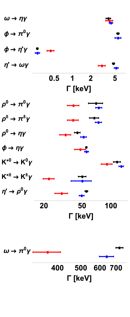
Figure 1: Comparison of the decay rates at leading order (red, middle entries) and at next-to-leading order in scenario II (blue, lower entries) with the experimental results (black, upper entries).

Table 7: Decay rates using the second scenario described in the text together with the deviations $\delta_{1}$ and $\delta_{2}$ of Eqs. (40).

Decay	$\Gamma_{\mathrm{PDG}}$ (keV)	$\Gamma_{\mathrm{NLO}}$ (keV)	deviation $\delta_{1}$	deviation $\delta_{2}$
$\rho^{0}\rightarrow\pi^{0}\gamma$	$70.\pm 12.$	$74.8\pm 5.7$	$0.066$	$0.35$
$\rho^{\pm}\rightarrow\pi^{\pm}\gamma$	$67.1\pm 7.5$	$74.2\pm 5.7$	$0.11$	$0.76$
$\rho^{0}\rightarrow\eta\gamma$	$44.7\pm 3.1$	$51.9\pm 3.7$	$0.16$	$1.5$
$\omega\rightarrow\pi^{0}\gamma$	$723.\pm 25.$	$640.\pm 44.$	$-0.11$	$-1.6$
$\omega\rightarrow\eta\gamma$	$3.91\pm 0.35$	$4.31\pm 0.28$	$0.10$	$0.89$
$\phi\rightarrow\pi^{0}\gamma$	$5.61\pm 0.26$	$5.65\pm 0.64$	$0.007$	$0.060$
$\phi\rightarrow\eta\gamma$	$55.4\pm 1.1$	$55.7\pm 2.7$	$0.005$	$0.093$
$\phi\rightarrow\eta^{\prime}\gamma$	$0.2643\pm 0.0090$	$0.265\pm 0.022$	$-0.002$	$-0.017$
$K^{\ast 0}\rightarrow K^{0}\gamma$	$116.\pm 10.$	$128.3\pm 7.2$	$0.11$	$1.0$
$K^{\ast\pm}\rightarrow K^{\pm}\gamma$	$50.4\pm 4.6$	$50.\pm 12.$	-	-
$\eta^{\prime}\rightarrow\rho^{0}\gamma$	$55.5\pm 1.9$	$49.6\pm 3.0$	$-0.11$	$-1.7$
$\eta^{\prime}\rightarrow\omega\gamma$	$4.74\pm 0.20$	$5.26\pm 0.39$	$0.11$	$1.2$

In Table 8, we present the correlation coefficients $\langle\delta c_{i}\delta c_{j}\rangle/(\delta c_{i}\delta c_{j})$ for our best fit of Table 7. As one might expect, the strongest correlation exists between parameters $c_{1}$ and $c_{+}$, because the linear combination $\tilde{c}_{1}=c_{1}+2M_{\pi}^{2}c_{+}$ contributes to all decays. There is also an equally strong correlation between $c_{1}$ and $c_{2}$. The parameter $c_{2}$ only contributes to the transitions between the vector-meson singlet and the pseudoscalar-meson octet. There is a slightly smaller correlation between $c_{2}$ and $c_{+}$. Finally, the last notable correlations exist between the parameter $\Lambda_{1}$, which is of order $1/N_{c}$, and the parameters $c_{1}$ and $c_{3}$. The remaining correlations are negligibly small.

Table 8: Off-diagonal array containing the correlation coefficients $\langle\delta c_{i}\delta c_{j}\rangle/(\delta c_{i}\delta c_{j})$ of the parameters $c_{i}$ for the fit of Table 7.

$c_{2}$	$\quad-0.73$
$c_{3}$	$\quad 0.033$	$0.14$
$c_{+}$	$\quad-0.78$	$0.46$	$0.16$
$c_{-}$	$\quad 0.21$	$-0.16$	$0.020$	$-0.13$
$\Lambda_{1}$	$\quad 0.50$	$-0.19$	$0.50$	$-0.29$	$0.11$
	$c_{1}$	$c_{2}$	$c_{3}$	$c_{+}$	$c_{-}$

IV.4 Expansion of the quark-charge matrix in $1/N_{c}$

As our final example, we also include the expansion of the quark-charge matrix in 1/$N_{c}$ [see Eq. (18)]. As a consequence of this expansion, also the $c_{4}$ interaction Lagrangian of Eq. (22) contributes to the invariant amplitudes (see Table 15 of Appendix A). Using the expressions of Table 15 of Appendix A and applying scenario II of Sec. IV.3, we obtain the results shown in Table 9. In fact, this scenario provides us with one additional parameter and it is therefore not surprising that $\chi^{2}_{\text{red}}=2.8$ (5 degrees of freedom) is smaller than the corresponding value $\chi^{2}_{\text{red}}=6.6$ of Table 6. The parameters of the fit are given by

$$\begin{split}c_{1}&=0.0536\pm 0.0013,\quad c_{2}=-0.000613\pm 0.000078,\quad c_{3}=0.00109\pm 0.00027,\\ c_{4}&=0.00142\pm 0.00055,\quad c_{+}=\left(1.05\pm 0.45\right)\cdot 10^{-9}\,\mathrm{MeV}^{-2},\quad c_{-}=\left(5.1\pm 1.6\right)\cdot 10^{-9}\,\mathrm{MeV}^{-2},\\ \Lambda_{1}&=0.247\pm 0.032.\end{split}$$ (42)

In Figure 2, we present a visual comparison of the decay rates at NLO in scenario II (blue, middle entries) and at NLO including a quark-charge expansion (green, lower entries) with the experimental results (black, upper entries). Except for the decays $\rho^{0}\to\eta\gamma$ and $K^{\ast 0}\to K^{0}\gamma$, we obtain an excellent agreement between experiment and theory.

Table 9: Decay rates using the second scenario described in the text, including an expansion of the quark-charge matrix in $1/N_{c}$. For the mixing angles we made use of the NLO values $\theta_{V}=39.8\degree$ and $\theta_{P}^{[1]}=-12.4\degree$. $\chi^{2}_{\mathrm{red}}=2.8$ (5 degrees of freedom).

Decay	$\Gamma_{\mathrm{PDG}}$ (keV)	$\Gamma_{\mathrm{mod}}$ in keV	$\delta_{1}$	$\delta_{2}$
$\rho^{0}\rightarrow\pi^{0}\gamma$	$70.\pm 12.$	$65.5\pm 5.6$	$-0.066$	$-0.35$
$\rho^{\pm}\rightarrow\pi^{\pm}\gamma$	$67.1\pm 7.5$	$65.0\pm 5.6$	$-0.031$	$-0.23$
$\rho^{0}\rightarrow\eta\gamma$	$44.7\pm 3.1$	$51.5\pm 2.4$	$0.15$	$1.7$
$\omega\rightarrow\pi^{0}\gamma$	$723.\pm 25.$	$689.\pm 30.$	$-0.047$	$-0.87$
$\omega\rightarrow\eta\gamma$	$3.91\pm 0.35$	$3.80\pm 0.44$	$-0.028$	$-0.19$
$\phi\rightarrow\pi^{0}\gamma$	$5.61\pm 0.26$	$5.69\pm 0.43$	$0.014$	$0.16$
$\phi\rightarrow\eta\gamma$	$55.4\pm 1.1$	$55.0\pm 1.8$	$-0.0070$	$-0.18$
$\phi\rightarrow\eta^{\prime}\gamma$	$0.2643\pm 0.0090$	$0.266\pm 0.015$	$0.0058$	$0.090$
$K^{\ast 0}\rightarrow K^{0}\gamma$	$116.\pm 10.$	$138.6\pm 5.2$	$0.19$	$2.0$
$K^{\ast\pm}\rightarrow K^{\pm}\gamma$	$50.4\pm 4.6$	$50.4\pm 7.9$	-	-
$\eta^{\prime}\rightarrow\rho^{0}\gamma$	$55.5\pm 1.9$	$53.4\pm 2.4$	$-0.038$	$-0.69$
$\eta^{\prime}\rightarrow\omega\gamma$	$4.74\pm 0.20$	$4.87\pm 0.31$	$0.027$	$0.34$

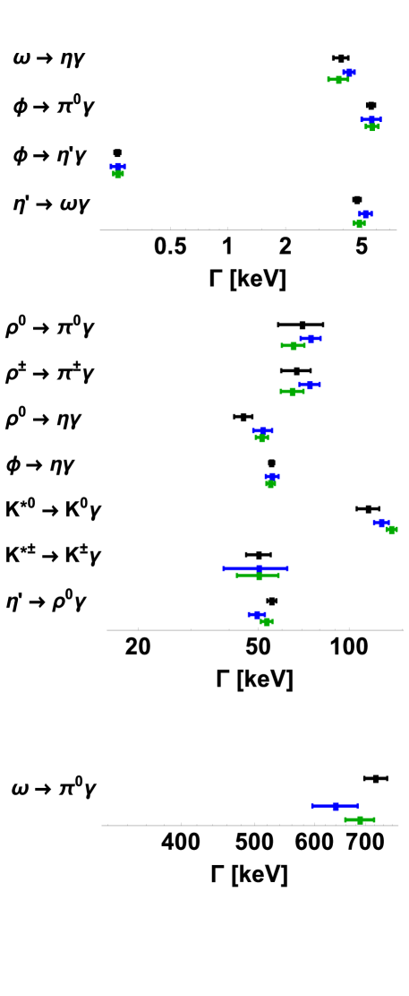
Figure 2: Comparison of the decay rates at next-to-leading order in scenario II (blue, middle entries), next-to-leading order including a $1/N_{c}$ expansion of the quark-charge matrix (green, lower entries) with the experimental results (black, upper entries).

IV.5 Coupling constants and convergence

We have organized the Lagrangians in terms of $1/N_{c}$ and the quark masses $m$ (contained in the quantities $\chi_{\pm}$). For the number of colors we insert $N_{c}=3$ and, with respect to the quark-mass expansion, we consider $M_{K}^{2}/(4\pi F)^{2}\approx 1/4$ as a typical small dimensionless expansion parameter, where $\Lambda_{\chi}=4\pi F$ denotes the chiral-symmetry-breaking scale Manohar:1983md . In Table 10, we collect the coupling constants as obtained from fitting the data using different levels of approximation. The second column (LO) refers to the leading-order Lagrangian with $\theta_{P}=\theta_{P}^{[0]}=-19.7\degree$ and ideal $\phi$-$\omega$ mixing, the third column (LO+$1/N_{c}$) to the leading-order Lagrangian plus $1/N_{c}$ corrections with $\theta_{P}=\theta_{P}^{[0]}=-19.7\degree$ and ideal $\phi$-$\omega$ mixing, the fourth column to the complete next-to-leading-order Lagrangian without expanding the quark-charge matrix $Q$ (NLO), and the fifth column to the complete next-to-leading-order Lagrangian including an expansion of $Q$ (NLO, $Q$ expanded). The last two scenarios made use of $\theta_{P}=\theta_{P}^{[1]}=-12.4\degree$, $\theta_{V}=39.8\degree$, and physical values for $F_{\pi}$ and $F_{K}$. As can be seen by comparing Tables 14 and 15 of Appendix A, the contributions of the coefficients $c_{i}$ to the decay matrix elements are redistributed in the version including the expansion of the quark-charge matrix. This is then the reason why, except for $c_{1}$, the coefficients differ notably for the last two cases.

Table 10: Coupling constants determined at leading order (LO), leading order plus $1/N_{c}$ corrections, next-to-leading order (NLO), and next-to-leading order with expanded quark-charge matrix (NLO, $Q$ expanded). See text for details.

Coupling constant	LO	LO+$1/N_{c}$	NLO	NLO, $Q$ expanded
$c_{1}$ $\left[10^{-2}\right]$	$3.82\pm 0.25$	$3.36\pm 0.20$	$5.22\pm 0.20$	$5.36\pm 0.13$
$c_{2}$ $\left[10^{-2}\right]$	-	$0.67\pm 0.10$	$-0.100\pm 0.021$	$-0.0613\pm 0.0078$
$c_{3}$ $\left[10^{-2}\right]$	-	$-0.39\pm 0.25$	$0.272\pm 0.072$	$0.109\pm 0.027$
$c_{4}$ $\left[10^{-2}\right]$	-	-	-	$0.142\pm 0.055$
$c_{+}$ $\left[10^{-2}\,\mathrm{GeV}^{-2}\right]$	-	-	$0.280\pm 0.078$	$0.105\pm 0.045$
$c_{-}$ $\left[10^{-2}\,\mathrm{GeV}^{-2}\right]$	-	-	$-0.61\pm 0.39$	$0.51\pm 0.16$

Finally, we would like to comment on the order of magnitude of the corrections in comparison with the leading-order term. We multiply the constants $c_{2}$, $c_{3}$, and $c_{4}$ by a factor of 3 to obtain the coefficients belonging to the $1/N_{c}$ expansion. Similarly, we multiply $c_{+}$ and $c_{-}$ by $(4\pi F)^{2}$ to obtain the coefficients for the dimensionless quark-mass expansion. The results corresponding to the last two columns of Table 10 are shown in Table 11.

Table 11: Expansion coefficients at next-to-leading order (NLO) corresponding to the last two columns of Table 10. For simplicity we suppress uncertainties.

Coefficients	physical $Q$	$Q$ expanded
$\tilde{c}_{1}$ [$10^{-2}$]	$5.23$	$5.36$
$c_{2}\cdot N_{c}$ [$10^{-2}$]	$-0.30$	$-0.18$
$c_{3}\cdot N_{c}$ [$10^{-2}$]	$0.82$	$0.33$
$c_{4}\cdot N_{c}$ [$10^{-2}$]	-	$0.43$
$c_{+}\cdot\left(4\pi F\right)^{2}$ [$10^{-2}$]	$0.36$	$0.14$
$c_{-}\cdot\left(4\pi F\right)^{2}$ [$10^{-2}$]	$-0.79$	$0.67$

Let us have a closer look at the implications of the second column of Table 11 (NLO with physical quark-charge matrix $Q$). We notice that all of the amplitudes ${\cal A}_{i}$ of Eq. (44) except for ${\cal A}_{5}$ start with $c_{1}$. We multiply each ${\cal A}_{i}$ ($i\neq 5$) with a suitable factor such that the leading-order term is simply given by $c_{1}$. We can then easily identify the amount of the largest relative correction. Regarding the $1/N_{c}$ terms, this is $3c_{2}/(2c_{1})$ for the amplitudes ${\cal A}_{9}$ and ${\cal A}_{11}$ and $3c_{3}/(2c_{1})$ for the amplitudes ${\cal A}_{7}$ and ${\cal A}_{10}$, respectively. Using the values of the second column of Table 11, we obtain $-0.086$ and $0.23$, respectively, where we have neglected the uncertainties. Keeping in mind that these numbers still have to be multiplied by 1/3, the $1/N_{c}$ corrections turn out to be relatively small, namely $-2.9$% and 7.8%, respectively. For the quark-mass corrections, the largest correction originating from $c_{+}$ is found in the ${\cal A}_{4}$ amplitude, namely, the ratio $16|c_{+}|(4\pi F)^{2}/(3c_{1})=0.37$ which gets multiplied by $(M_{K}^{2}-M_{\pi}^{2})/(4\pi F)^{2}=0.17$. The relative quark-mass correction of 6.3% is of a similar magnitude as the $1/N_{c}$ correction. More pronounced is the case of the $c_{-}$ coupling, resulting in the ratio $6|c_{-}|(4\pi F)^{2}/c_{1}=0.90$ which, together with the factor $(M_{K}^{2}-M_{\pi}^{2})/(4\pi F)^{2}=0.17$, gives rise to a relative correction of 15%. Recall that this parameter is entirely determined by the decay $K^{\ast\pm}\to K^{\pm}\gamma$. For the third column of Table 11 (NLO with expanded quark-charge matrix $Q$), we obtain similar results.

IV.6 Comparison with other calculations in chiral effective Lagrangian approaches

Reference Klingl:1996by contains the leading-order Lagrangian of the vector formulation for the $VP\gamma$ decay of neutral vector mesons into neutral pions. When comparing this with Eq. (3.19) of Ref. Klingl:1996by , we agree after identifying our $2ec_{1}/F$ with $d/f_{\pi}$ of Ref. Klingl:1996by . However, their Eq. (4.7) for the decay rates seems to contain an error, namely, the second line needs to be multiplied by a factor of 1/9, originating from the elements of the quark-charge matrix in the form $(2/3-1/3)^{2}$. Accordingly, the coupling $d\simeq 0.01$ of Eq. (4.10) needs to be multiplied by a factor of 3. Similarly, our results from the leading-order Lagrangian agree with the coefficients reported in Fig. 3 of Ref. Danilkin:2017lyn , which, beyond SU(3) symmetry, implicitly made use of nonet symmetry in combination with ideal $\phi$-$\omega$ mixing and neglected $\eta$-$\eta^{\prime}$ mixing.

The antisymmetric tensor-field representation Kyriakopoulos:1969zm ; Kyriakopoulos:1973pt was used in, e.g., Refs. RuizFemenia:2003hm ; Lutz:2008km ; Terschlusen:2012xw ; Chen:2013nna for the calculation of the $VP\gamma$ interaction. In Ref. RuizFemenia:2003hm , the relevant interaction Lagrangian for the interaction of two vector fields with one pseudoscalar field ($VVP$) and for one vector resonance with an external vector field and a pseudoscalar field ($VJP$) was constructed, involving $7+4$ coupling constants, respectively. In terms of the QCD short-distance behavior of the $VVP$ Green function, constraints among the coupling constants were derived. Using these constraints, Eq. (4.2) of Ref. RuizFemenia:2003hm provides a parameter-free prediction for the $\omega\to\pi^{0}\gamma$-transition matrix element, translating into a prediction for our $c_{1}$,

$$|c_{1}|=\frac{1}{4\sqrt{2}}\left(\frac{3}{8\pi^{2}}\frac{m_{\omega}}{F}-\frac{F}{2}\frac{m_{\omega}}{m_{V}^{2}}\right).$$

Using $F=90.9$ MeV and $m_{\omega}=m_{V}=782.7$ MeV, one obtains $|c_{1}|=4.76\times 10^{-2}$ which has to be compared with our LO prediction $|c_{1}|=(3.82\pm 0.25)\times 10^{-2}$ and the NLO prediction $|c_{1}|=(5.22\pm 0.20)\times 10^{-2}$ of Table 10. In Ref. Lutz:2008km , antisymmetric tensor fields were used for describing the radiative decays of the vector-meson nonet into the pseudoscalar octet. The $\eta^{\prime}$ was not considered, the physical $\eta$ was taken as part of the pseudoscalar octet, and for the $\phi$-$\omega$ system an ideal mixing was assumed. The decay proceeds either via a $VVP$ vertex such that the propagating neutral vector meson subsequently couples to a real photon or via a direct $VP\gamma$ interaction (which is considered to be of higher order in their chiral counting). The decay rates then contain three (combinations of) coupling constants, namely $e_{A}$ (direct decay), $h_{A}e_{V}$ and $b_{A}e_{V}$ (indirect decay) [see Eqs. (38)-(42) of Ref. Lutz:2008km ]. In the limit of SU(3) symmetry, our results for the invariant amplitudes fully agree with those of Ref. Lutz:2008km . To see this, one needs to set all vector-meson masses equal to $m_{V}$, all pseudoscalar meson masses equal to $\overline{M}$, $F=f$, and, finally, $e|\tilde{c}_{1}|=|\tilde{e}_{A}|/8$, where $\tilde{e}_{A}=e_{A}+\frac{1}{4}h_{A}e_{V}-2b_{A}e_{V}\overline{M}^{2}/m_{V}^{2}$. In Ref. Terschlusen:2012xw , the analysis was extended to also include the $\eta^{\prime}$ meson. With two additional parameters, namely, the $\eta$-$\eta^{\prime}$ mixing angle $\theta_{P}$ and one parameter $b_{H}$ for the interaction of the singlet eta with two vector mesons, in total five parameters were adjusted to five decays. In particular, an unconventionally small mixing angle $\theta_{P}\simeq\pm 2\degree$ was found. When taking SU(3)-symmetry breaking effects into account, in our framework two additional parameters are available, namely, $c_{+}$ and $c_{-}$, whereas in the framework of Ref. Lutz:2008km only the combination $b_{A}e_{V}$ will give rise to SU(3)-symmetry breaking effects. This term corresponds to our $c_{+}$ structure. In particular, the SU(3) relation $|{\cal A}_{K^{\ast 0}\to K^{0}\gamma}|=2|{\cal A}_{K^{\ast\pm}\to K^{\pm}\gamma}|$ will not be broken in the framework of Ref. Lutz:2008km , unless higher-order terms are taken into account. In our calculation, the parameter $c_{-}$ decouples ${\cal A}_{K^{\ast\pm}\to K^{\pm}\gamma}$ and ${\cal A}_{K^{\ast 0}\to K^{0}\gamma}$. On the other hand, in Ref. Chen:2013nna , the importance of such a term in the context of SU(3) symmetry breaking was already worked out for the radiative $K^{\ast}\to K\gamma$ decays. Reference Chen:2013nna extended the results of RuizFemenia:2003hm by also including excited vector-meson resonances.

Recently, Kimura, Morozumi, and Umeeda Kimura:2016xnx investigated decays of light hadrons within a chiral Lagrangian model that includes both the lightest pseudoscalar and vector mesons. As an extension of chiral perturbation theory, they included one-loop corrections due to the Goldstone bosons and the corresponding counter terms. In addtion to other processes, they also particularly looked at the $VP\gamma$ reactions. For the decays involving the light vector mesons, the model provides three parameters.

In Table 12, we provide a comparison of our results with those of Ref. Kimura:2016xnx . First of all, we note that, with the exception of the decays $\omega\to\pi^{0}\gamma$ and $K^{\ast 0}\to K^{0}\gamma$, our central values for the decay rates agree better with the experimental values than those from Ref. Kimura:2016xnx . In addition, the uncertainties from Ref. Kimura:2016xnx are, on average, much larger than ours. We conclude that our approach provides an improved description of the $VP\gamma$ decays.

Table 12: Comparison of our results at NLO with the predictions of Ref. Kimura:2016xnx (KMU18).

Decay	$\Gamma_{\mathrm{exp}}$ [keV]	$\Gamma_{\mathrm{NLO}}$ [keV]	$\Gamma_{\mathrm{KMU18}}$ [keV]
$\rho^{0}\rightarrow\pi^{0}\gamma$	$70.\pm 12.$	$65.5\pm 5.6$	$46.\pm 5.$
$\rho^{\pm}\rightarrow\pi^{\pm}\gamma$	$67.1\pm 7.5$	$65.0\pm 5.6$	$73.\pm 7.$
$\rho^{0}\rightarrow\eta\gamma$	$44.7\pm 3.1$	$51.5\pm 2.4$	$33.^{+8.}_{-9.}$
$\omega\rightarrow\pi^{0}\gamma$	$723.\pm 25.$	$689.\pm 30.$	$710.\pm 90.$
$\omega\rightarrow\eta\gamma$	$3.91\pm 0.35$	$3.80\pm 0.44$	$5.5^{+1.6}_{-1.3}$
$\phi\rightarrow\pi^{0}\gamma$	$5.61\pm 0.26$	$5.69\pm 0.43$	$17.^{+12.}_{-9.}$
$\phi\rightarrow\eta\gamma$	$55.4\pm 1.1$	$55.0\pm 1.8$	$22.^{+9.}_{-12.}$
$\phi\rightarrow\eta^{\prime}\gamma$	$0.2643\pm 0.0090$	$0.266\pm 0.015$	$0.39^{+0.12}_{-0.09}$
$K^{\ast 0}\rightarrow K^{0}\gamma$	$116.\pm 10.$	$138.6\pm 5.2$	$110.\pm 10.$
$K^{\ast\pm}\rightarrow K^{\pm}\gamma$	$50.4\pm 4.6$	$50.4\pm 7.9$	$28.\pm 3.$
$\eta^{\prime}\rightarrow\rho^{0}\gamma$	$55.5\pm 1.9$	$53.4\pm 2.4$	-
$\eta^{\prime}\rightarrow\omega\gamma$	$4.74\pm 0.20$	$4.87\pm 0.31$	$4.6^{+3.3}_{-2.0}$

V summary

In this work we analyzed the radiative transitions between the vector-meson nonet and the pseudoscalar-meson nonet within a chiral effective Lagrangian approach. For that purpose we have determined the Lagrangian up to and including the next-to-leading order in an expansion in $1/N_{c}$ and the quark masses. For the transformation behavior of the vector mesons under the Lorentz group we made use of the vector representation. At leading order, the Lagrangian contains one free parameter which was determined from a simultaneous fit to 11 experimental decay rates. (The decay $\phi\to\pi^{0}\gamma$ was excluded because of the OZI rule.) Both $\eta$-$\eta^{\prime}$ and $\phi$-$\omega$ mixing were taken into account at leading order. The results of this scenario are given in Table 3 and clearly show that a good description of all experimental data at leading order is not possible. We then gradually improved the model by first taking into account $1/N_{c}$ corrections (see Table 4) and then also quark mass corrections (see Table 5), which introduced 2 plus 2 additional parameters, respectively. In this context, we also had to consider the corrections due to the wavefunction renormalization and the mixing at NLO. As a result, another parameter of the $\eta$-$\eta^{\prime}$ system was included in the calculation, which served as a further fit parameter. Then fits were carried out in which either the invariant amplitude or the decay were expanded up to and including next-to-leading order (scenario I and II, respectively). From Table 6 we concluded that the second scenario yields a better description of the experimental data. In Figure 2 we provided a visual presentation of the improvement from LO to NLO. However, one has to keep in mind in this context that at leading order only one free parameter is available to describe 11 decays, while at NLO 6 parameters (including $\Lambda_{1}$) have been fitted to 12 decays. In our final fit we made use of a $1/N_{c}$ expansion of the quark-charge matrix, which gives rise to one additional free parameter and results in the best description of the data (see Table 9 and Fig. 2). We also found that the contributions to the amplitudes ${\cal A}_{i}$ of Eq. (44), which are generated by the $1/N_{c}$ and the quark mass corrections, are smaller in magnitude than 15% of the leading-order term. In other words, they can really be regarded as corrections. Clearly, our approach is limited in the sense that extending it to include even NNLO corrections would introduce a number of additional parameters such that there would be no more predictive power. However, it would be interesting to see how pseudoscalar-meson loop corrections affect our findings Krasniqi . In summary, we can say that the present calculation is the most comprehensive investigation of the $VP\gamma$ decays to date and provides a satisfactory description of the experimental decay rates.

Appendix A Lagrangians

Let us introduce the following structures involving the singlet and octet fields:

$$T_{1\rho\sigma} =\rho^{+}_{\rho}\partial_{\sigma}\pi^{-}+\rho^{-}_{\rho}\partial_{\sigma}\pi^{+}+\rho^{0}_{\rho}\partial_{\sigma}\pi^{0},$$

$$T_{2\rho\sigma} =K^{\ast+}_{\rho}\partial_{\sigma}K^{-}+K^{\ast-}_{\rho}\partial_{\sigma}K^{+},$$

$$T_{3\rho\sigma} =\overline{K}^{\ast 0}_{\rho}\partial_{\sigma}K^{0}+K^{\ast 0}_{\rho}\partial_{\sigma}\overline{K}^{0},$$

$$T_{4\rho\sigma} =\omega_{8\rho}\partial_{\sigma}\eta_{8},$$

$$T_{5\rho\sigma} =\omega_{1\rho}\partial_{\sigma}\eta_{1},$$

$$T_{6\rho\sigma} =\rho^{0}_{\rho}\partial_{\sigma}\eta_{8},$$

$$T_{7\rho\sigma} =\rho^{0}_{\rho}\partial_{\sigma}\eta_{1},$$

$$T_{8\rho\sigma} =\omega_{8\rho}\partial_{\sigma}\pi^{0},$$

$$T_{9\rho\sigma} =\omega_{1\rho}\partial_{\sigma}\pi^{0},$$

$$T_{10\rho\sigma} =\omega_{8\rho}\partial_{\sigma}\eta_{1},$$

$$T_{11\rho\sigma} =\omega_{1\rho}\partial_{\sigma}\eta_{8}.$$ (43)

The effective Lagrangian of the $VP\gamma$ interaction may then be written as

$${\cal L}_{\rm eff}^{VP\gamma}=e\epsilon^{\mu\nu\rho\sigma}F_{\mu\nu}\sum_{i=1}^{11}{\cal A}_{i}T_{i\rho\sigma}.$$ (44)

Defining

$$E^{\rho\sigma} \equiv 2\frac{e}{F}\epsilon^{\rho\sigma\mu\nu}F_{\mu\nu},$$

$$H_{\rho\sigma} \equiv\Big{[}(Q_{u}+Q_{d})T_{1\rho\sigma}+(Q_{u}+Q_{s})T_{2\rho\sigma}+(Q_{d}+Q_{s})T_{3\rho\sigma}$$

$$\quad+\frac{1}{3}(Q_{u}+Q_{d}+4Q_{s})T_{4\rho\sigma}+\frac{2}{3}(Q_{u}+Q_{d}+Q_{s})T_{5\rho\sigma}$$

$$\quad+(Q_{u}-Q_{d})\left(\frac{1}{\sqrt{3}}T_{6\rho\sigma}+\sqrt{\frac{2}{3}}T_{7\rho\sigma}+\frac{1}{\sqrt{3}}T_{8\rho\sigma}+\sqrt{\frac{2}{3}}T_{9\rho\sigma}\right)$$

$$\quad+\frac{\sqrt{2}}{3}(Q_{u}+Q_{d}-2Q_{s})(T_{10\rho\sigma}+T_{11\rho\sigma})\Big{]},$$

where $Q_{u}$, $Q_{d}$, and $Q_{s}$ denote the quark charges, the Lagrangian of Eq. (20) is given by

$${\cal L}^{VP\gamma}_{\text{LO}}=c_{1}E^{\rho\sigma}H_{\rho\sigma}.$$ (45)

The charge factors are given in Table 13 both for the physical charges and their values as $N_{c}\to\infty$. Note that the $T_{5\rho\sigma}$ term does not contribute for physical values of the quark charges.

Table 13: Charge factors for physical values and the limit $N_{c}\to\infty$.

	Physical value	value as $N_{c}\to\infty$
$Q_{u}$	$\frac{2}{3}$	$\frac{1}{2}$
$Q_{d}$	$-\frac{1}{3}$	$-\frac{1}{2}$
$Q_{s}$	$-\frac{1}{3}$	$-\frac{1}{2}$
$Q_{u}+Q_{d}$	$\frac{1}{3}$	$0$
$Q_{u}+Q_{s}$	$\frac{1}{3}$	$0$
$Q_{d}+Q_{s}$	$-\frac{2}{3}$	$-1$
$Q_{u}-Q_{d}$	$1$	$1$
$Q_{u}+Q_{d}+4Q_{s}$	$-1$	$-2$
$Q_{u}+Q_{d}-2Q_{s}$	$1$	$1$
$Q_{u}+Q_{d}+Q_{s}$	$0$	$-\frac{1}{2}$

The $1/N_{c}$ corrections are given by

$${\cal L}^{VP\gamma}_{\text{NLO,$1/N_{c}$}} =E^{\rho\sigma}\left\{c_{2}\left[(Q_{u}+Q_{d}+Q_{s})T_{5\rho\sigma}+\sqrt{\frac{3}{2}}(Q_{u}-Q_{d})T_{9\rho\sigma}+\frac{1}{\sqrt{2}}(Q_{u}+Q_{d}-2Q_{s})T_{11\rho\sigma}\right]\right.$$

$$\quad+c_{3}\left[(Q_{u}+Q_{d}+Q_{s})T_{5\rho\sigma}+\sqrt{\frac{3}{2}}(Q_{u}-Q_{d})T_{7\rho\sigma}+\frac{1}{\sqrt{2}}(Q_{u}+Q_{d}-2Q_{s})T_{10\rho\sigma}\right]$$

$$\left.\vphantom{\sqrt{\frac{3}{2}}}\quad+c_{4}(Q_{u}+Q_{d}+Q_{s})(T_{1\rho\sigma}+T_{2\rho\sigma}+T_{3\rho\sigma}+T_{4\rho\sigma}+T_{5\rho\sigma})\right\}.$$ (46)

Since $\langle Q\rangle=Q_{u}+Q_{d}+Q_{s}=0$ for the physical quark charges, the last term does not contribute in this case. Furthermore, for physical quark charges, there is no singlet-to-singlet transition ($T_{5\rho\sigma}$). In order to express the quark mass corrections we make use of the leading-order kaon and pion masses squared Gasser:1984gg , $\mathring{M}^{2}_{K}=B_{0}\left(\hat{m}+m_{s}\right)$ and $\mathring{M}^{2}_{\pi}=2B_{0}\hat{m}$. To the order we are considering, we replace the leading-order expressions by the physical values, i.e., $\mathring{M}^{2}_{K}\to M_{K}^{2}$ and $\mathring{M}^{2}_{\pi}\to M_{\pi}^{2}$. The quark-mass corrections are then given by

$${\cal L}^{VP\gamma}_{\text{NLO,$\chi$}} =(2c_{5}-c_{7}-c_{8})E^{\rho\sigma}\Big{\{}M^{2}_{\pi}(Q_{u}+Q_{d})T_{1\rho\sigma}+[M^{2}_{\pi}Q_{u}+(2M_{K}^{2}-M_{\pi}^{2})Q_{s}]T_{2\rho\sigma}$$

$$\quad+[M^{2}_{\pi}Q_{d}+(2M_{K}^{2}-M_{\pi}^{2})Q_{s}]T_{3\rho\sigma}+\frac{1}{3}[M_{\pi}^{2}(Q_{u}+Q_{d})+4Q_{s}(2M_{K}^{2}-M_{\pi}^{2})]T_{4\rho\sigma}$$

$$\quad+\frac{2}{3}[M_{\pi}^{2}(Q_{u}+Q_{d})+(2M_{K}^{2}-M_{\pi}^{2})Q_{s}]T_{5\rho\sigma}$$

$$\quad+M_{\pi}^{2}(Q_{u}-Q_{d})\left(\frac{1}{\sqrt{3}}T_{6\rho\sigma}+\sqrt{\frac{2}{3}}T_{7\rho\sigma}+\frac{1}{\sqrt{3}}T_{8\rho\sigma}+\sqrt{\frac{2}{3}}T_{9\rho\sigma}\right)$$

$$\quad+\frac{\sqrt{2}}{3}[M_{\pi}^{2}(Q_{u}+Q_{d})-2(2M_{K}^{2}-M_{\pi}^{2})Q_{s}](T_{10\rho\sigma}+T_{11\rho\sigma})\Big{\}}$$

$$\quad+(2c_{6}-c_{7}+c_{8})E^{\rho\sigma}\Big{\{}M^{2}_{\pi}(Q_{u}+Q_{d})T_{1\rho\sigma}+[(2M_{K}^{2}-M_{\pi}^{2})Q_{u}+M^{2}_{\pi}Q_{s}]T_{2\rho\sigma}$$

$$\quad+[(2M_{K}^{2}-M_{\pi}^{2})Q_{d}+M^{2}_{\pi}Q_{s}]T_{3\rho\sigma}+\frac{1}{3}[M_{\pi}^{2}(Q_{u}+Q_{d})+4Q_{s}(2M_{K}^{2}-M_{\pi}^{2})]T_{4\rho\sigma}$$

$$\quad+\frac{2}{3}[M_{\pi}^{2}(Q_{u}+Q_{d})+(2M_{K}^{2}-M_{\pi}^{2})Q_{s}]T_{5\rho\sigma}$$

$$\quad+M_{\pi}^{2}(Q_{u}-Q_{d})\left(\frac{1}{\sqrt{3}}T_{6\rho\sigma}+\sqrt{\frac{2}{3}}T_{7\rho\sigma}+\frac{1}{\sqrt{3}}T_{8\rho\sigma}+\sqrt{\frac{2}{3}}T_{9\rho\sigma}\right)$$

$$\quad+\frac{\sqrt{2}}{3}[M_{\pi}^{2}(Q_{u}+Q_{d})-2(2M_{K}^{2}-M_{\pi}^{2})Q_{s}](T_{10\rho\sigma}+T_{11\rho\sigma})\Big{\}}.$$

Using $2M_{K}^{2}-M_{\pi}^{2}=M_{\pi}^{2}+2(M_{K}^{2}-M_{\pi}^{2})$ and noting that $Q_{d}=Q_{s}$, we may write

$${\cal L}^{VP\gamma}_{\text{NLO,$\chi$}} =2M_{\pi}^{2}(c_{5}+c_{6}-c_{7})E^{\rho\sigma}T_{\rho\sigma}$$

$$\quad+4(M_{K}^{2}-M_{\pi}^{2})(c_{5}+c_{6}-c_{7})E^{\rho\sigma}\Big{[}\frac{1}{2}(Q_{u}+Q_{s})T_{2\rho\sigma}+Q_{s}T_{3\rho\sigma}+\frac{4}{3}Q_{s}T_{4\rho\sigma}+\frac{2}{3}Q_{s}T_{5\rho\sigma}$$

$$\quad-2\frac{\sqrt{2}}{3}Q_{s}(T_{10\rho\sigma}+T_{11\rho\sigma})\Big{]}$$

$$\quad+2(M_{K}^{2}-M_{\pi}^{2})(c_{5}-c_{6}-c_{8})E^{\rho\sigma}(Q_{s}-Q_{u})T_{2\rho\sigma}.$$ (47)

In Table 14, we collect the amplitudes ${\cal A}_{i}$, $i=1,\ldots,11$, of Eq. (44). We have defined $c_{+}=c_{5}+c_{6}-c_{7}$, $c_{-}=c_{5}-c_{6}-c_{8}$, and $\tilde{c}_{1}=c_{1}+2M_{\pi}^{2}c_{+}$. The results depend on 5 parameters $c_{1}$ ($\tilde{c}_{1}$), $c_{2}$, $c_{3}$, $c_{+}$, and $c_{-}$.

Table 14: Amplitudes ${\cal A}_{i}$ for the full result in units of $2/F$; $c_{+}=c_{5}+c_{6}-c_{7}$, $c_{-}=c_{5}-c_{6}-c_{8}$, $\tilde{c}_{1}=c_{1}+2M_{\pi}^{2}c_{+}$.

Transition	structure	amplitude ${\cal A}_{i}$ in units of $2/F$
$\rho\to\pi\gamma$	$T_{1}$	$\frac{1}{3}\tilde{c}_{1}$
$K^{\ast\pm}\to K^{\pm}\gamma$	$T_{2}$	$\frac{1}{3}\tilde{c}_{1}+\frac{2}{3}(M_{K}^{2}-M_{\pi}^{2})c_{+}-2(M_{K}^{2}-M_{\pi}^{2})c_{-}$
$K^{\ast}\to K^{0}\gamma$	$T_{3}$	$-\frac{2}{3}\tilde{c}_{1}-\frac{4}{3}(M_{K}^{2}-M_{\pi}^{2})c_{+}$
$\omega_{8}\to\eta_{8}\gamma$	$T_{4}$	$-\frac{1}{3}\tilde{c}_{1}-\frac{16}{9}(M_{K}^{2}-M_{\pi}^{2})c_{+}$
$\omega_{1}\to\eta_{1}\gamma$	$T_{5}$	$-\frac{8}{9}(M_{K}^{2}-M_{\pi}^{2})c_{+}$
$\rho^{0}\to\eta_{8}\gamma$	$T_{6}$	$\frac{1}{\sqrt{3}}\tilde{c}_{1}$
$\rho^{0}\to\eta_{1}\gamma$	$T_{7}$	$\sqrt{\frac{2}{3}}\,\tilde{c}_{1}+\sqrt{\frac{3}{2}}\,c_{3}$
$\omega_{8}\to\pi^{0}\gamma$	$T_{8}$	$\frac{1}{\sqrt{3}}\tilde{c}_{1}$
$\omega_{1}\to\pi^{0}\gamma$	$T_{9}$	$\sqrt{\frac{2}{3}}\,\tilde{c}_{1}+\sqrt{\frac{3}{2}}\,c_{2}$
$\omega_{8}\to\eta_{1}\gamma$	$T_{10}$	$\frac{\sqrt{2}}{3}\tilde{c}_{1}+\frac{1}{\sqrt{2}}c_{3}+\frac{8\sqrt{2}}{9}(M_{K}^{2}-M_{\pi}^{2})c_{+}$
$\omega_{1}\to\eta_{8}\gamma$	$T_{11}$	$\frac{\sqrt{2}}{3}\tilde{c}_{1}+\frac{1}{\sqrt{2}}c_{2}+\frac{8\sqrt{2}}{9}(M_{K}^{2}-M_{\pi}^{2})c_{+}$

In Table 15, we collect the corresponding coefficients of the large-$N_{c}$ expansion. We show the results at leading order (LO) and at next-to-leading order (NLO), depending on one parameter and six parameters, respectively.

Table 15: Amplitudes ${\cal A}_{i}$ in the large-$N_{c}$ expansion in units of $2/F$; $c_{+}=c_{5}+c_{6}-c_{7}$, $c_{-}=c_{5}-c_{6}-c_{8}$.

Structure	amplitude ${\cal A}_{i}$ at LO in $[2/F]$	amplitude ${\cal A}_{i}$ at NLO in $[2/F]$
$T_{1}$	0	$\frac{1}{3}c_{1}-\frac{1}{2}c_{4}$
$T_{2}$	0	$\frac{1}{3}c_{1}-\frac{1}{2}c_{4}-2(M_{K}^{2}-M_{\pi}^{2})c_{-}$
$T_{3}$	$-c_{1}$	$-\frac{2}{3}c_{1}-\frac{1}{2}c_{4}-2M_{K}^{2}c_{+}$
$T_{4}$	$-\frac{2}{3}c_{1}$	$-\frac{1}{3}c_{1}-\frac{1}{2}c_{4}-\frac{4}{3}(2M_{K}^{2}-M_{\pi}^{2})c_{+}$
$T_{5}$	$-\frac{1}{3}c_{1}$	$-\frac{1}{2}c_{2}-\frac{1}{2}c_{3}-\frac{1}{2}c_{4}-\frac{2}{3}(2M_{K}^{2}-M_{\pi}^{2})c_{+}$
$T_{6}$	$\frac{1}{\sqrt{3}}c_{1}$	$\frac{1}{\sqrt{3}}c_{1}+\frac{2}{\sqrt{3}}M_{\pi}^{2}c_{+}$
$T_{7}$	$\sqrt{\frac{2}{3}}\,c_{1}$	$\sqrt{\frac{2}{3}}\,c_{1}+\sqrt{\frac{3}{2}}\,c_{3}+2\sqrt{\frac{2}{3}}\,M_{\pi}^{2}c_{+}$
$T_{8}$	$\frac{1}{\sqrt{3}}c_{1}$	$\frac{1}{\sqrt{3}}c_{1}+\frac{2}{\sqrt{3}}M_{\pi}^{2}c_{+}$
$T_{9}$	$\sqrt{\frac{2}{3}}\,c_{1}$	$\sqrt{\frac{2}{3}}\,c_{1}+\sqrt{\frac{3}{2}}\,c_{2}+2\sqrt{\frac{2}{3}}M_{\pi}^{2}c_{+}$
$T_{10}$	$\frac{\sqrt{2}}{3}c_{1}$	$\frac{\sqrt{2}}{3}c_{1}+\frac{1}{\sqrt{2}}c_{3}+\frac{2}{3}\sqrt{2}(2M_{K}^{2}-M_{\pi}^{2})c_{+}$
$T_{11}$	$\frac{\sqrt{2}}{3}c_{1}$	$\frac{\sqrt{2}}{3}c_{1}+\frac{1}{\sqrt{2}}c_{2}+\frac{2}{3}\sqrt{2}(2M_{K}^{2}-M_{\pi}^{2})c_{+}$

References

- (1) J. Gasser and H. Leutwyler, Phys. Rep. 87, 77 (1982).
- (2) J. Goldstone, Nuovo Cim. 19, 154 (1961).
- (3) J. Goldstone, A. Salam, and S. Weinberg, Phys. Rev. 127, 965 (1962).
- (4) G. ’t Hooft, Nucl. Phys. B 72, 461 (1974).
- (5) E. Witten, Nucl. Phys. B 160, 57 (1979).
- (6) P. Di Vecchia and G. Veneziano, Nucl. Phys. B 171, 253 (1980).
- (7) S. R. Coleman and E. Witten, Phys. Rev. Lett. 45, 100 (1980).
- (8) S. L. Adler, Phys. Rev. 177, 2426 (1969).
- (9) J. S. Bell and R. Jackiw, Nuovo Cim. A 60, 47 (1969).
- (10) G. ’t Hooft, Phys. Rev. Lett. 37, 8 (1976).
- (11) E. Witten, Nucl. Phys. B 156, 269 (1979).
- (12) G. Veneziano, Nucl. Phys. B 159, 213 (1979).
- (13) S. Weinberg, Physica A 96, 327 (1979).
- (14) J. Gasser and H. Leutwyler, Annals Phys. 158, 142 (1984).
- (15) J. Gasser and H. Leutwyler, Nucl. Phys. B 250, 465 (1985).
- (16) J. F. Donoghue, E. Golowich, and B. R. Holstein, Dynamics of the Standard Model (Cambridge University Press, Cambridge, 1992).
- (17) S. Scherer, Adv. Nucl. Phys. 27, 277 (2003).
- (18) S. Scherer and M. R. Schindler, Lect. Notes Phys. 830, 1 (2012).
- (19) B. Moussallam, Phys. Rev. D 51, 4939 (1995).
- (20) H. Leutwyler, Phys. Lett. B 374, 163 (1996).
- (21) P. Herrera-Siklody, J. I. Latorre, P. Pascual, and J. Taron, Nucl. Phys. B 497, 345 (1997).
- (22) R. Kaiser and H. Leutwyler, Eur. Phys. J. C 17, 623 (2000).
- (23) H. Leutwyler, Nucl. Phys. Proc. Suppl. 64, 223 (1998).
- (24) R. Kaiser and H. Leutwyler, in Nonperturbative Methods in Quantum Field Theory (World Scientific, Singapore, 1998).
- (25) P. Herrera-Siklody, Phys. Lett. B 442, 359 (1998).
- (26) B. Borasoy, Eur. Phys. J. C 34, 317 (2004).
- (27) X. K. Guo, Z. H. Guo, J. A. Oller, and J. J. Sanz-Cillero, JHEP 1506, 175 (2015).
- (28) P. Bickert, P. Masjuan, and S. Scherer, Phys. Rev. D 95, 054023 (2017).
- (29) J. Gasser, M. E. Sainio, and A. Švarc, Nucl. Phys. B 307, 779 (1988).
- (30) E. E. Jenkins and A. V. Manohar, Phys. Lett. B 255, 558 (1991).
- (31) J. Bijnens, P. Gosdzinsky, and P. Talavera, JHEP 9801, 014 (1998).
- (32) T. Becher and H. Leutwyler, Eur. Phys. J. C 9, 643 (1999).
- (33) J. Gegelia and G. Japaridze, Phys. Rev. D 60, 114038 (1999).
- (34) T. Fuchs, J. Gegelia, G. Japaridze, and S. Scherer, Phys. Rev. D 68, 056005 (2003).
- (35) P. C. Bruns and U.-G. Meissner, Eur. Phys. J. C 40, 97 (2005).
- (36) M. F. M. Lutz and S. Leupold, Nucl. Phys. A 813, 96 (2008).
- (37) D. Djukanovic, J. Gegelia, A. Keller, and S. Scherer, Phys. Lett. B 680, 235 (2009).
- (38) S. Weinberg, Phys. Rev. 166, 1568 (1968).
- (39) S. R. Coleman, J. Wess, and B. Zumino, Phys. Rev. 177, 2239 (1969).
- (40) C. G. Callan, Jr., S. R. Coleman, J. Wess, and B. Zumino, Phys. Rev. 177, 2247 (1969).
- (41) O. Kaymakcalan, S. Rajeev, and J. Schechter, Phys. Rev. D 30, 594 (1984).
- (42) O. Kaymakcalan and J. Schechter, Phys. Rev. D 31, 1109 (1985).
- (43) M. Bando, T. Kugo, and K. Yamawaki, Nucl. Phys. B 259, 493 (1985).
- (44) U.-G. Meißner, Phys. Rep. 161, 213 (1988).
- (45) M. Bando, T. Kugo, and K. Yamawaki, Phys. Rep. 164, 217 (1988).
- (46) G. Ecker, J. Gasser, A. Pich, and E. de Rafael, Nucl. Phys. B 321, 311 (1989).
- (47) G. Ecker, J. Gasser, H. Leutwyler, A. Pich, and E. de Rafael, Phys. Lett. B 223, 425 (1989).
- (48) M. C. Birse, Z. Phys. A 355, 231 (1996).
- (49) M. Harada and K. Yamawaki, Phys. Rep. 381, 1 (2003).
- (50) K. Kampf, J. Novotny, and J. Trnka, Eur. Phys. J. C 50, 385 (2007).
- (51) D. Djukanovic, J. Gegelia and S. Scherer, Int. J. Mod. Phys. A 25, 3603 (2010).
- (52) S. Weinberg, The Quantum Theory of Fields. Vol. 1: Foundations (Cambridge University Press, Cambridge, England, 1995).
- (53) L. H. Ryder, Quantum Field Theory (Cambridge University Press, Cambridge, 1985).
- (54) E. Kyriakopoulos, Phys. Rev. 183, 1318 (1969).
- (55) E. Kyriakopoulos, Phys. Rev. D 6, 2202 (1972).
- (56) S. L. Glashow, Phys. Rev. Lett. 11, 48 (1963).
- (57) P. J. O’Donnell, Rev. Mod. Phys. 53, 673 (1981).
- (58) V. V. Anisovich, A. A. Anselm, Y. I. Azimov, G. S. Danilov, and I. T. Dyatlov, Phys. Lett. 16, 194 (1965).
- (59) C. Becchi and G. Morpurgo, Phys. Rev. 140, B687 (1965).
- (60) J. W. Durso, Phys. Lett. B 184, 348 (1987).
- (61) I. Danilkin, O. Deineka, and M. Vanderhaeghen, Phys. Rev. D 96, 114018 (2017).
- (62) H. Gomm, O. Kaymakcalan, and J. Schechter, Phys. Rev. D 30, 2345 (1984).
- (63) O. Hajuj, Z. Phys. C 60, 357 (1993).
- (64) F. Klingl, N. Kaiser, and W. Weise, Z. Phys. A 356, 193 (1996).
- (65) M. Benayoun, L. DelBuono, S. Eidelman, V. N. Ivanchenko, and H. B. O’Connell, Phys. Rev. D 59, 114027 (1999).
- (66) P. D. Ruiz-Femenía, A. Pich, and J. Portolés, JHEP 0307, 003 (2003).
- (67) C. Terschlüsen, S. Leupold, and M. F. M. Lutz, Eur. Phys. J. A 48, 190 (2012).
- (68) Y.-H. Chen, Z.-H. Guo, and H.-Q. Zheng, Phys. Rev. D 90, 034013 (2014).
- (69) D. Kimura, T. Morozumi, and H. Umeeda, Prog. Theor. Exp. Phys. 2018, 123B02 (2018).
- (70) S.-l. Zhu, W-Y. P. Hwang and Z.-s. Yang, Phys. Lett. B 420, 8 (1998)
- (71) A. Gokalp and O. Yilmaz, Eur. Phys. J. C 24, 117 (2002).
- (72) C. Aydin, M. Bayar, and A. H. Yilmaz, Phys. Rev. D 81, 094032 (2010).
- (73) R. M. Woloshyn, Z. Phys. C 33, 121 (1986).
- (74) M. Crisafulli and V. Lubicz, Phys. Lett. B 278, 323 (1992).
- (75) C. J. Shultz, J. J. Dudek, and R. G. Edwards, Phys. Rev. D 91, 114501 (2015).
- (76) B. J. Owen, W. Kamleh, D. B. Leinweber, M. S. Mahbub and B. J. Menadue, Phys. Rev. D 92, 034513 (2015).
- (77) C. Alexandrou et al., Phys. Rev. D 98, 074502 (2018).
- (78) O. Bär and U. J. Wiese, Nucl. Phys. B 609, 225 (2001).
- (79) R. K. Bhaduri, Models of the Nucleon: From Quarks to Soliton (Addison-Wesley, Redwood City, CA, 1988), Sec. 5.6.
- (80) A. V. Manohar, in Probing the Standard Model of Particle Interactions. Proceedings of the Les Houches Summer School, Session 68, edited by R. Gupta, A. Morel, E. de Rafael, and F. David (Elsevier, Amsterdam, 1999), Pt. 1 and 2.
- (81) H. W. Fearing and S. Scherer, Phys. Rev. D 53, 315 (1996).
- (82) P. A. Zyla et al. (Particle Data Group), Prog. Theor. Exp. Phys. 2020, 083C01 (2020) and 2021 update.
- (83) J. D. Bjorken and S. D. Drell, Relativistic Quantum Mechanics (McGraw-Hill, New York, 1964).
- (84) C. Itzykson and J. B. Zuber, Quantum Field Theory (McGraw-Hill, New York, 1980).
- (85) J. Bijnens and G. Ecker, Ann. Rev. Nucl. Part. Sci. 64, 149 (2014).
- (86) Wolfram Research, Inc., Mathematica, Version 11.0, Champaign, IL (2016).
- (87) S. Okubo, Phys. Lett. 5, 165 (1963).
- (88) G. Zweig, CERN Report Nos. TTH-401 and TH-412, 1964 (unpublished).
- (89) J. Iizuka, Prog. Theor. Phys. Suppl. 37, 21 (1966).
- (90) A. Manohar and H. Georgi, Nucl. Phys. B 234, 189 (1984).
- (91) A. Krasniqi, H. C. Lange, and S. Scherer, work in progress.