Improving the Solar Wind Density Model Used in Processing of Spacecraft Ranging Observations

Abstract

Solar wind plasma as a cause of radio signal delay has been playing an important role in solar and planetary science. Early experiments studying the distribution of electrons near the Sun from spacecraft ranging measurements were designed so that the radio signal was passing close to the Sun. At present, processing of spacecraft tracking observations serves a different goal: precise (at meter level) determination of orbits of planets, most importantly Mars. Solar wind adds a time-varying delay to those observations, which is, in this case, unwanted and must be subtracted prior to putting the data into planetary solution. Present planetary ephemeris calculate the delay assuming symmetric stationary power-law model of solar wind density. The present work, based on a custom variant of the EPM lunar-planetary ephemeris, raises the question of accuracy and correctness of that assumption and examines alternative models based on in situ solar wind density data provided by OMNI and on the ENLIL numerical model of solar wind.

1 Introduction

Two-frequency observations of the Viking spacecraft in 1976 (lander and orbiter) were once used for analysis of radio signal propagation delays due to solar wind plasma (Callahan, 1977; Muhleman & Anderson, 1981). Also, there were plans for dual-frequency ranging for the Mars Express spacecraft (Patzold et al., 2004; Remus et al., 2014), but no information is known about the outcome. Apart from those, the spacecraft tracking measurements are made on single frequency, thus determining the delay in solar wind directly from the measurements themselves is not possible. While, in principle, other radio observations could help, such as VLBI (Aksim et al., 2019) or observations of scintillations or radio sources (Shishov et al., 2016), in practice there are too few of them, and even fewer, if any, on the dates of spacecraft tracking measurements. Three options remain for accounting for delay in solar wind when determining planetary orbits for ephemeris:

1. Using a simplified model of solar wind electron density distribution, and then determining its single free parameter (a reference electron density) from the spacecraft tracking observations.

2. Using in situ electron density measurements done by spacecraft such as the Advanced Composition Explorer (ACE) and Wind, to account for large-scale temporal variations of the said electron density in the interplanetary space, while keeping a simplified symmetric model for electron density distribution at any moment.

3. Using a more complicated dynamical model of solar wind, which accounts for corotating interaction regions existing in solar wind. Such models of the solar wind are often built on top of models of solar corona, whose parameters are fit to magnetograms, either daily or mean (averaged over one solar cycle). This approach does not necessarily preclude using the in situ data.

The symmetric models most often include the term of electron density proportional to $1/r^{2}$, where $r$ is the distance to the center of the Sun. This term assumes constant radial velocity of electrons. The factor of this term (reference electron density) is a free parameter of the model that is determined from spacecraft ranging observations.

While all modern planetary ephemeris (DE, EPM, INPOP) use the $1/r^{2}$ density, their approaches differ in details. DE200 (Standish, 1990) used the following model for solar wind correction of Mariner ranges:

$$N_{\mathrm{e}}=\frac{A}{r^{6}}+\frac{B}{r^{2}},$$

where $A$ is a fitted parameter and $B$ depends on solar latitude $\beta$:

$$B=\frac{ab}{a^{2}\sin^{2}\beta+b^{2}\cos^{2}\beta}$$

($a$ and $b$ are fitted parameters as well). DE430 (Folkner et al., 2014) presumably uses a similar model, where the parameters are determined per-planet or per-spacecraft.

In EPM2004 (Pitjeva, 2004) and subsequent releases of EPM, the following model was used:

$$N_{\mathrm{e}}=\frac{A}{r^{6}}+\frac{B+\dot{B}t}{r^{2}},$$ (1)

where $A$ was fixed to the value determined in DE200, and $B$ with its linear drift $\dot{B}$ were determined from observations, per-planet, per-year.

INPOP presumably has two models that are used interchangeably (Verma et al., 2013): (i) a two-parameter model with one term proportional to $1/r^{2}$ and the other proportional to $1/r^{4}$; (ii) a two-parameter model with the term proportional to $1/r^{\epsilon}$, where $\epsilon$ is the second determined parameter. The parameters are fit per each solar conjunction of each planet of interest, and also separately for spacecraft being in the fast-wind zone and in the slow-wind zone.

Outside planetary ephemeris, other solar wind electron density models exist; see e.g. Leblanc et al. (1998) where $1/r^{2}$, $1/r^{4}$, and $1/r^{6}$ terms are combined. However, the $1/r^{4}$ and higher order terms have negligible effect on spacecraft tracking signals that pass farther than 15 solar radii ($15R_{\odot}$) from the center of the Sun. The signals that pass closer than that cannot be used for precise orbit determination anyway because of the temporal and spatial instabilities of the delay in solar wind in such proximity.

There exist other models with fractional powers of $r$ close to 2, see e.g. Bougeret et al. (1984) with $r^{-2.10}$, Mann et al. (1999) with $r^{-2.16}$, or Verma et al. (2013) with values of $\epsilon$ ranging from 2.10 to 2.50. Such models in general do not possess physical meaning and, as we will now show, do not offer prospects of more accurate representation of spacecraft signal delay.

A major problem in determination of solar wind parameters from spacecraft ranges (aside from the temporal, latitudinal, and longitudinal variations) is that not only the factor of the $1/r^{2}$ (or $1/r^{\epsilon}$) term must be determined from observations, but the whole set of parameters that form the ephemeris solution. Those include parameters of orbits of the planets, mass of the Sun, masses of dozens of asteroids, and, most importantly, signal delays (biases) that come from spacecraft transponder going out of calibration and from systematic errors of signal registration in radio observatories (Kuchynka et al., 2012).

In fact, just having one factor and one offset to fit for the delay of spacecraft ranges in solar wind already makes the power of $r$ largely irrelevant. Figure 6 in Appendix B provides an example where $1/r^{2.5}$ model is fitted to data generated using the $1/r^{2}$ model well enough for practical purposes.

We emphasise that there is no power law that can be preferable in a symmetric model of solar wind electron density — either from the position of physical principles or from the position of processing of signal delays.

1.1 Medium-term density variations

Medium-term variations in the solar wind are ones that have duration similar to the period of solar rotation (Sun’s synodic rotation period is 27.2753 days). One obvious problem with the approach of using the $1/r^{2}$ model is the assumption that solar wind is radially symmetric. The asymmetry of the solar wind can be clearly seen, for instance, in the LASCO coronagraph images. The fact that spacecraft ranging observations are sensitive enough to be affected by this asymmetry was reported by Kuchynka et al. (2012), who analyzed 10-day rolling averages of the observation residuals and noticed the presence of periodic variations with a period of 27 days. (See Appendix A for brief introduction to radio ranging residuals).

The way to account for these periodic variations is to adopt, instead of the $1/r^{2}$ model, a three-dimensional numerical model of the solar wind that would simulate (to some level of agreement) the corotating structures of the solar wind based on observations of the Sun.

In this work, we examine the results obtained with the WSA-ENLIL model, which consists of two parts: the ENLIL solar wind model (Odstrcil, 2003) and the WSA (Wang–Sheeley–Arge, Wang & Sheeley Jr, 1990; Arge & Pizzo, 2000; Sheeley Jr, 2017) model of the solar corona.

ENLIL is a magnetohydrodynamic (MHD) solar wind model that calculates 3D distributions of solar wind’s density, velocity, and magnetic field by solving a system of differential MHD equations using a coronal solution given by WSA as a boundary condition at 0.1 AU. WSA is a semi-empirical solar corona model that uses line-of-sight magnetic field measurements of the solar photosphere assembled into synoptic magnetograms and simulates the solar wind plasma outflow up to 0.1 AU.

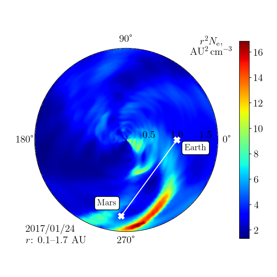
Figure 1: Normalized solar wind electron number density calculated by WSA-ENLIL with daily-updated GONGz magnetograms. The data are plotted in the helio-equatorial plane with latitude of 0° in the HEEQ coordinate system (see Thompson, 2006).

The primary purpose of WSA-ENLIL is prediction of solar wind structures reaching Earth (and, with the help of the CONE model, prediction of geomagnetic storms caused by coronal mass ejections). However, there is no reason the model cannot be used for other purposes, such as processing of spacecraft ranging observations.

Figure 1 shows WSA-ENLIL density distributions in the solar equatorial plane for January 24 and May 10, 2017. The spiral shapes in the map are corotating solar wind structures.

1.2 Long-term density variations

Along with previously mentioned 27-day periodic variations in solar wind’s density, there are also long-term variations that happen on a larger scale, i.e. on a scale of years. These long-term variations can be seen by analysing in situ density measurements applying a rolling average filter with a window size large enough to smooth out any medium-term data variations.

Figure 2 shows 365-day rolling average of the solar wind electron density at 1 AU calculated twice: (i) from the OMNI dataset (Papitashvili et al., 2014; King & Papitashvili, 2005) using values of proton density and alpha–proton ratio and assuming charge neutrality (see Section 3.2), and (ii) from the ENLIL simulations (see Section 3.3). The plot reveals that the average electron density in the long term can deviate up to 20% from its mean value, so the assumption of some “nominal” electron density for all time would be unjustified in the processing of spacecraft radio ranges.

Our suggestion is that these long-term variations must be taken into account regardless of the particular solar wind model used. Specifically, if the power-law model like $N_{0}/r^{2}$ is used, one constant $N_{0}$ multiplier would result in constant density at 1 AU, which would not be in agreement with in situ observations. Therefore, $N_{0}$ must be made proportional to in situ density smoothed in a way that would eliminate any medium-term disturbances and variations, such as 27-day periodic ones resulting from the Sun’s rotation.

In the case of ENLIL, we have to take into account the inner workings of the model (Odstrcil, 2004). First, we must note that ENLIL assumes that the electron and proton densities are equal. Also, it is important that to calculate the density at the inner boundary, ENLIL requires that at $r=0.1$ AU the condition of constant momentum flux holds:

$$N_{\mathrm{e}}(\vartheta,\varphi)\,v_{r}^{2}(\vartheta,\varphi)=d_{\mathrm{fast}}^{\phantom{1}}\cdot v_{\mathrm{fast}}^{2}=\mathrm{const},$$ (2)

in which $v_{r}(\vartheta,\varphi)$ is the radial velocity distribution produced by the WSA solar corona model, $N_{\mathrm{e}}(\vartheta,\varphi)$ is the density distribution further used as the boundary condition, and $d_{\mathrm{fast}}$ and $v_{\mathrm{fast}}$ are free model parameters named dfast and vfast. Presumably, parameters $d_{\mathrm{fast}}$ and $v_{\mathrm{fast}}$ should be adjusted so that the solution matches observational data. If great precision is not a requirement, this adjustment may be performed post factum, i.e. by directly scaling the solution $N_{\mathrm{e}}(r,\vartheta,\varphi)$.

The WSA-ENLIL average density curve shown in Figure 2 was calculated with fixed values of $d_{\mathrm{fast}}$ and $v_{\mathrm{fast}}$, i.e. with one constant value of momentum flux. The figure shows that when momentum flux is fixed, WSA-ENLIL’s average electron density at 1 AU (i) is not constant and (ii) does not match the OMNI numbers.

Quite obviously, with average density being non-constant, simply setting $d_{\mathrm{fast}}$ proportional to electron density derived from OMNI would do very little to bring the two curves in agreement. Instead, knowing that variations in density are defined by variations in WSA velocity, we presume that the first step should be to use values of $v_{\mathrm{fast}}$ based on WSA velocity distribution $v_{r}(\vartheta,\varphi)$, possibly choosing the distribution’s average as the parameter’s value. Doing so would produce solutions with near-constant average density at 1 AU, and, at that stage, $d_{\mathrm{fast}}$ may be set to values proportional to OMNI density. Such a setup should, in theory, produce solutions that match observational in situ data.

However, since ENLIL simulations require time to complete and solutions may be scaled post factum, the simplest (and the one used in this work) way to bring ENLIL data in agreement with OMNI is to remove the density trend shown in Figure 2 directly from the solution $N_{\mathrm{e}}(t,r,\vartheta,\varphi)$ and to apply to the data the same procedure as we do to $N_{0}$ parameter of the $N_{0}/r^{2}$ model.

Figure 2: Solar wind electron density at 1 AU (365-day rolling average), years 2006–2017.

For a detailed description of the in situ data used, see Section 3.2.

2 Radio signal propagation in solar wind

Radio signal propagation velocity in plasma is defined by the group refractive index (Aksim et al., 2019)

$$n_{\mathrm{gr}}(\mathbf{r},\omega)\approx 1+\frac{N_{\mathrm{e}}(\mathbf{r})}{2\,N_{\mathrm{crit}}(\omega)},$$ (3)

where $\omega$ is the signal’s angular frequency, $N_{\mathrm{e}}(\mathbf{r})$ is the plasma’s electron number density, and $N_{\mathrm{crit}}(\omega)=m_{\mathrm{e}}\,\varepsilon_{0}\,\omega^{2}/e^{2}$ is critical plasma density ($e$ is the charge of electron, and $\varepsilon_{0}$ is the vacuum permittivity).

To calculate the time it takes for a radio signal of frequency $\omega$ to travel through the solar wind plasma from the point given by position vector $\mathbf{r}_{a}$ to the point $\mathbf{r}_{b}$, one has to integrate the plasma’s group refractive index $n_{\mathrm{gr}}(\mathbf{r},\omega)$ along the straight line connecting $\mathbf{r}_{a}$ and $\mathbf{r}_{b}$, that is, to evaluate the integral

$$\begin{split}\tau&=\int_{\mathbf{r}_{a}}^{\mathbf{r}_{b}}n_{\mathrm{gr}}(s,\omega)\,\mathrm{d}s=\\ &=|\mathbf{r}_{b}-\mathbf{r}_{a}|+\frac{1}{2\,N_{\mathrm{crit}}(\omega)}\int_{\mathbf{r}_{a}}^{\mathbf{r}_{b}}N_{\mathrm{e}}(s)\,\mathrm{d}s=\tau_{\mathrm{dist}}+\tau_{\mathrm{cor}}.\end{split}$$ (4)

The term $\tau_{\mathrm{dist}}$ in the above expression corresponds to the time delay due to the distance between $\mathbf{r}_{a}$ and $\mathbf{r}_{b}$, i.e. the time it would take for the signal to travel the same path in vacuum, and $\tau_{\mathrm{cor}}$ is the additional dispersive time delay due to the lower propagation velocity in solar wind.

In the case of a power-law electron density model $N_{\mathrm{e}}(r)\propto r^{\alpha}$ the integral in Equation 4 may be expressed in closed form (see Aksim et al., 2019). In the general case, specifically if the electron density is defined by a grid of numerical values, which is the case with ENLIL and other numerical models, the integral has to be evaluated numerically. To calculate the integral numerically, we used the Simpson’s rule (Kahaner et al., 1989, sec. 5.1) with step size of 0.00625 AU, equal to the radial grid spacing of the used simulation data (see Section 3.3), which allows to exclude possible error originating from the grid.

3 Data

Despite this work being focused on Mars spacecraft observations, each of the considered solar wind models was tested as part of its respective planetary solution. Each solution was fit not only to Mars spacecraft observations, but to the full set of observations usually required to build ephemeris, including not only spacecraft ranging, but also optical observations and other kinds of observations. For details, we refer the reader to (Pitjeva, 2013; Pitjeva & Pitjev, 2014).

3.1 Spacecraft ranges

The Mars spacecraft ranges that were crucial to this work were taken from the webpage of Solar System Dynamics (SSD) group at NASA JPL, which includes Mars Global Surveyor (MGS, 1999–2006), Odyssey (2002–2013), and Mars Reconnaissance Orbiter (MRO, 2006–2013). The extended set of ranges for MRO and Odyssey up to the end of 2017 was kindly provided by William Folkner. The provided ranges are normal points (NPs) made from raw observations. A normal point represents the distance from an Earth radio observatory to the center of Mars, corrected for the delay in ionosphere and troposphere.

Following the decision from (Kuchynka et al., 2012), pre-2005 Odyssey and MRO ranges acquired by Deep Space Network stations 26 and 43 were removed from analysis, as well as ranges acquired by station 54 before October 2008.

MGS, Odyssey, and MRO ranges that pass closer than 30$R_{\odot}$ to the Sun suffer too much from solar wind instabilities and have been removed from analysis. Ranges that pass farther than 30$R_{\odot}$, but closer than 60$R_{\odot}$ have been treated separately (but equally with other ranges).

Mars Express (MEX) and Venus Express (VEX) ranges (Morley & Budnik, 2009) that are also sensitive to the delay in solar wind were downloaded from the Geoazur website. They too are published as observatory–Mars distances corrected for ionosphere and troposphere, but otherwise they are “raw” observations, so normal points had to be made from them before processing. VEX ranges between 23.08.2010 and 31.10.2010 were excluded from analysis due to poor residuals, the reason believed to be bad orbit determination due to trajectory control maneuvers being more frequent than usual; VEX ranges between 02.10.2011 and 05.12.2011 were excluded too, assuming the same reason. Due to generally big noise in VEX residuals, the decision was made to exclude VEX ranges that pass closer than $90R_{\odot}$ to the Sun, so that they do not interfere with less noisy observations in the comparison of the solar wind models. The MEX ranges were treated similarly to Odyssey and MRO, with the cutoff values of $30R_{\odot}$ and $60R_{\odot}$.

MESSENGER (2011–2014, Park et al., 2017) and Cassini (2004–2014) spacecraft ranges (normal points) were also taken from the aforementioned SSD webpage; however, the published values have been already reduced for the delay in solar wind (calculated by the JPL DE solar wind model), so they did not participate directly in the analysis of solar wind models. However, those observations are very important for Solar system ephemeris as a whole; in particular, they reduce the uncertainty of the mass of the Sun.

In this work, different models of solar wind plasma electron density are compared in their application to building planetary ephemeris. One of the models, WSA-ENLIL, depends (in its WSA part) on the GONG magnetograms that did not exist before September 2006 (see Section 3.3), so the comparison is done for 2006–2017. The spacecraft observations that touch this time span are summarized in Table 1. The reception (Rx) and transmission (Tx) frequencies are listed so as to emphasise that the frequency is important for calculation of the delay of radio signal in plasma, see Equation 3.

Table 1: Spacecraft observations used in the comparison of solar wind models. NPs = normal points, Rx = reception, Tx = transmission, $\sigma$ = a priori error

Spacecraft	Time span	# of NPs		$\sigma$, one-way	Frequency
		$>60R_{\odot}$	$30..60R_{\odot}$		Rx	Tx
Odyssey	2002–2017	7988	1784	0.5 m	7155 MHz	8407 MHz
MRO	2006–2017	1924	561	0.5 m	7183 MHz	8439 MHz
MEX	2005–2015	2888	718	1.5 m	7100 MHz	8400 MHz
VEX	2006–2013	1294†	—	3 m	7166 MHz	8419 MHz
† Sun–signal distance for all VEX normal points is greater than $90R_{\odot}$.

3.2 In situ solar wind measurements

Low-resolution (daily) version of the NASA/GSFC’s OMNI dataset was used as the source of in situ data in this work. The dataset is combined from in situ data measured by multiple spacecraft. The ones that serve as sources of the particle density data for 2006–2017 are the ACE (Stone et al., 1998) and Wind (Wilson III et al., 2021).

OMNI provides proton density $N_{\mathrm{p}}$ and alpha–proton ratio $N_{\mathrm{a}}/N_{\mathrm{p}}$. To calculate electron density $N_{\mathrm{e}}$, we used the plasma quasi-neutrality condition $N_{\mathrm{e}}=N_{\mathrm{p}}+N_{\mathrm{a}}/2$.

The daily density data provided by OMNI are volatile because of the nature of the solar wind structures; see the “raw” electron density data derived from OMNI on Figure 3. Since we are interested in the (average) electron density along the signal path, our analysis can not benefit from the information about the daily variations at the end of the signal path (near Earth). On the other hand, we assume that a sufficiently smoothed electron density curve will represent long-term variations of electron density of the solar wind in the whole inner Solar system, including the Earth–Mars line. The Savitzky–Golay filter (Savitzky & Golay, 1964) was chosen as one of the most widely used filters for time series. The parameters of the filter were chosen in an ad hoc manual procedure: the window of 511 days and the polynomial order 5. The filtered data are shown on Figure 3.

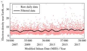
Figure 3: OMNI data of electron density near Earth, years 2006–2017. The filter used is Savitzky–Golay with a window of 511 days and the polynomial order 5.

Alternatively to OMNI, in situ electron density data are also provided by the ESA/NASA Solar and Heliospheric Observatory (SOHO, Hovestadt et al., 1995). This data is not part of the OMNI combination. The results obtained with the SOHO data (not shown in the text) turned out to be somewhat worse than the ones obtained with OMNI.

3.3 Numerical solar wind density maps

WSA-ENLIL data were produced by request via the “Runs on Request” service on the Community Coordinated Modeling Center (CCMC) website. The whole dataset covers the dates between September 2006 and December 2017 and consists of 12 separate runs, each one covering one year.

The grid size in the WSA-ENLIL runs was set to $256\times 10\times 90\ (r\times\vartheta\times\phi)$ with grid boundaries 0.1…1.7 AU, $-$20°…+20° latitude, 0°…360° longitude (in HEEQ coordinate system). The grid spacing, therefore, is 0.00625 AU in radial direction and 4° in latitudinal and longitudinal directions. The output frequency for the simulations was set to once every 12 hours.

The solar surface magnetic field data used for WSA coronal solutions consisted of daily updated synoptic maps produced by the Global Oscillation Network Group (GONG, Hill, 2018).

It must be noted that there are two kinds of GONG magnetograms, called GONGb and GONGz. They were supposed to be identical with the only difference that GONGz has non-solar magnetic field bias removed. However, it was found in late 2015 that GONGz magnetograms suffered from over-subtraction in the polar regions. The correction of the over-subtraction gradually went into effect starting from August 2016 and reaching all GONG stations in April 2017. Unfortunately, it is not possible to retroactively correct the past GONGz data (Mays et al., 2020, sec. 5.4). So the numerical simulations in 2017 and later are expected to be more accurate when GONGz is used; before 2017, the expected improvement of GONGz is not reached and GONGb is more accurate.

4 Analysis

As said above, a full planetary ephemeris solution were obtained for each of the considered solar wind models. All solutions were based on EPM and ERA-8 software (Pavlov & Skripnichenko, 2015).

4.1 Dynamical model

EPM has a single dynamical model of the Solar system that includes all planets, the Moon, the Sun, asteroids (see section 4.2), discrete model of Kuiper belt (160 uniformly distributed points of equal mass) and 30 individual trans-Neptunian objects (Pitjeva & Pitjev, 2018b). Sixteen bodies (the Sun, the planets, Pluto, Ceres, Pallas, Vesta, Iris, Bamberga) obey Einstein–Infeld–Hoffmann equations of motion. Other bodies, for the sake of performance, interact with those 16 bodies with only Newtonian forces, and do not interact with each other. It has been checked that taking into account the full set of relativistic interactions affects the Earth–Mars distance by a few centimeters, which is negligible with the present observations.

Apart from point-mass interactions, the model includes additional accelerations from solar oblateness and Lense–Thirring effect. Earth also gets “point mass–figure” accelerations that come from the Sun, Venus, Mars, Jupiter, and the Moon (Pavlov et al., 2016).

The planetary part of the EPM model has over 600 parameters that are determined simultaneously in the least-squares fit (see Appendix A). Here are the parameters that are important for the analysis of radio ranges from Earth to Mars orbiters:

• orbital elements for all planets at epoch,

• solar oblateness factor,

• masses of 279 asteroids,

• distance scale parameter, historically known as correction to the value of AU,

• single factor of electron density, which applies to delay in solar wind plasma,

• biases to compensate for calibration errors or clock offsets on Earth or on spacecraft: 15 per-station biases for MGS/Odyssey, 14 per-station biases for MRO, single transponder delay for MGS, single transponder delay for Mars Express.

The distance scale parameter represents the correction to $GM_{\odot}$—the mass of the Sun. It is numerically harder to determine the mass of the Sun directly because of correlations with semi-major axes of planets. Determination of $GM_{\odot}$ (and, in specific solutions, its time derivative) allows to study the physical properties of the Sun and to test general relativity (Pitjeva et al., 2021).

It is important to process different kinds of observations simultaneously to get realistic values of parameters and error estimates. For example, MESSENGER observations help greatly to determine the solar oblateness factor, because Mercury is close to the Sun. The solar oblateness factor affects orbits of Earth and Mars. To determine the distance scaling factor, one has to take ranging data for MESSENGER, MEX, Mars orbiters, and Cassini. Earth’s orbit, whose precision is obviously important for processing of the Earth–Mars ranges, depends on the Moon’s orbit around Earth, which is determined from lunar laser ranging observations. Optical observations are important for determination of orbits of Uranus and Neptune, who in turn affect Mars’s orbit on long time spans.

4.2 Perturbing asteroids

An important part of the model, especially in regard to the Mars spacecraft observations, are the point-masses that represent the asteroids in the Main Asteroid Belt. In EPM2017, 301 largest asteroids were present in the dynamical model; the remaining part of the Main Asteroid Belt was modelled as a discrete rotating annulus consisting of 180 uniformly distributed points of equal mass (Pitjeva & Pitjev, 2018a; Pitjeva & Pavlov, 2017). Masses of 16 individual asteroids were fixed to the values determined from observations of spacecraft or natural satellites orbiting them; 30 masses were determined as part of ephemeris solution (i.e. by the perturbations that they inflict on orbits of inner planets); other asteroids’ masses were determined as mean densities of three taxonomic classes (C, S, M).

In the updated ephemeris dynamical model used in this work, the number of individual asteroids is 279. The source list of asteroids was merged (with obvious removal of duplicates) from 343 asteroids of the DE430 model (Folkner et al., 2014) and 287 asteroids from (Kuchynka et al., 2010, Table A.1). The former is believed to be the list of most perturbing asteroids, while the latter is believed to be the list of most “non-ring-like-acting” asteroids, i.e. their cumulative effect on inner planets cannot be modelled by a uniform ring. The resulting list contained 379 asteroids. Then, 100 asteroids whose masses were determined negative (though always within uncertainty) were excluded from the model. Such negative masses are an artifact of the least-squares method and they come from the fact that there is not enough observational data to properly determine them.

None of the 279 masses were fixed in planetary solutions in this work; rather, all of them were determined along with other planetary parameters by a weighted least-squares method enhanced with Tikhonov regularization (Kuchynka & Folkner, 2013; Kan & Pavlov, 2022). The a priori masses and uncertainties used in the regularization were taken from different sources. The masses of 17 asteroids are known with small uncertainties, thanks to observations of spacecraft or their natural satellites (comparing to EPM2017, binary asteroid Euphrosyne was added to the list). For 77 asteroids, the a priori values were the ones determined from observed deflections of orbits of other asteroids during close approach. For the remaining 285 asteroids, the estimates were taken based on diameters observed in infrared (Tedesco et al., 2004; Masiero et al., 2011) and densities assigned to the three taxonomic classes.

4.3 Solutions

Three solutions were made, with identical sets of observations and parameters, differing only in solar wind delay model for the time span of 2006–2017.

• In Solution I, the delays were calculated in accordance with the simplest model of electron density, symmetric and stationary: $N_{\mathrm{e}}=CN_{0}/r^{2}$, where $N_{0}$ (the reference electron density at $r=1$ AU) was made equal to the 2006–2017 time-average of OMNI data, which was found to be 5.97 cm^-3. The formal error of this average value was calculated to be 0.07 cm^-3 from the formal errors of the proton density and alpha/proton ratio: $\sigma(N_{\mathrm{p}})$ and $\sigma(N_{\mathrm{a}}/N_{\mathrm{p}})$. The single electron density factor $C$ (which works as the factor of delay, see the $\tau_{\mathrm{cor}}$ term in Equation 4) was fit to observations. Ideally, $C$ would be equal to 1; the purpose of $C$ is to account for uncertainty in the observed electron density, and also for the fact that the assumption of stationary electron density in 2006–2017 is not very realistic.

• In Solution II, the delays were calculated in accordance with a symmetric, but non-stationary electron density model: $N_{\mathrm{e}}=CN_{1}(t)/r^{2}$, where the function $N_{1}(t)$ is is equal to the smoothed electron density values derived from OMNI (see Section 3.2 and Figure 3). The single factor $C$ was fit to observations.

• In Solution III, the delays were calculated in accordance with the WSA-ENLIL model of electron density, scaled so that the (365-day rolling average of) electron density near Earth is equal to the smoothed OMNI values. Similarly to Solutions I and II, a single factor $C$ of the electron density was fit to observations.

The values of the fitted electron density factor $C$ in the three solutions are listed in Table 2. While its reference value is 1 in all solutions, there is a difference in how it is fitted. In Solution I, the $C$ was not constrained, since the assumption of stationary electron density in 2006–2017 is already not very realistic. In Solutions II and III, the Tikhonov regularization was used to effectively constrain $C$ so that its a priori standard deviation is 1.17%. The value was taken equal to the relative standard deviation of the electron density in the OMNI data (see the description of the Solution I above).

Pre-2006 spacecraft ranges, which include MGS and parts of Odyssey and MEX, were processed with the symmetric stationary solar wind model, with different factors fit for different periods of time between Sun–Mars conjunctions. One factor was fit for 2002/01/01—2003/12/31, another for 2004/01/01—2006/09/29.

A different factor was fit for pre-2002 MGS ranges. The same factor was used for pre-1990 radar observations of Mars, Mercury, and Venus, although they are hardly sensitive to delay in solar wind because of low accuracy.

5 Results

Figure 4 shows the residual (postfit) differences of Odyssey (blue points) and MRO (red points) ranges plus the values of the model delay in solar wind. For better visibility, only ranges from mid-2013 to mid-2017 are shown. The model delay in solar wind is shown separately with green curves, so that one can see how the model delay curve is fitted to observations.

The black curves show the time-averaged spacecraft range residuals. They have visible medium-term variations with period close to 27 days (the period changes as Earth and Mars move on their orbits; the vertical lines on Figure 4 are separated by the solar rotation period). The amplitude of variations increases near Sun–Mars conjunctions, which is expected because during the conjunctions, Earth–Mars signals pass close to the Sun, and at small distances from the Sun the electron density is higher than at large distances. Observations with signal passing closer than $30R_{\odot}$ to the Sun are not shown.

On the bottom plot of Figure 4 it can be seen that the WSA-ENLIL solar wind delay model expectedly has 27-day variations, too. In some cases there is a good match between peaks in the model and in the residuals, but often it goes “out of sync” or the amplitudes become very different. One explanation for this is the unfortunate fact that all the GONG magnetograms are obtained from Earth—and the daily-updated map of the magnetic field that is fed to the ENLIL’s MHD equations is correct only on the visible side of the Sun. On the nonvisible side, it is a prediction, often not a very accurate one.

Before 2017, we can also attribute the differences between WSA-ENLIL model data and real spacecraft delays to the GONGb magnetograms containing non-solar magnetic field bias (see Section 3.3). For 2017, when GONGz magnetograms were used, we support the first explanation with anecdotal evidence. A good match between WSA-ENLIL model and spacecraft data can be clearly seen on the bottom plot of Figure 4 in the first three months of 2017, while in the following three months, this is no longer the case. Figure 1 shows two example maps for the two quarters of 2017. One can see that on the first map, the corotating structures that intersect the Earth–Mars line originate from the visible half of the Sun’s surface; while on the second map, the Earth–Mars line has changed in the way that it is also intersected by a corotating structure whose origin is on the nonvisible half. (If the pictures were animated, the structures would rotate anticlockwise in time.) We admit that this can not be accepted as strong evidence and hope for a future possibility to analyze post-2017 spacecraft data together with WSA-ENLIL simulations based on properly fixed GONGz magnetograms.

The Mars Express data are shown in Figure 5. One can see, apart from the expected peaks with a period of approximately 27 days, long-term variations that far exceed the peaks. The cause of the variations certainly cannot be an inaccuracy of the EPM’s dynamical model of motion of Mars, or reductions, or solar wind delay model, because there are no variations of that magnitude in the Odyssey and MRO residuals. It is also unlikely that the variations come from a radio observatory on Earth: same Deep Space Network stations observe Mars Express, Odyssey and MRO spacecraft. The most reasonable explanation would be that there are problems in orbit determination for the spacecraft. In any case, the comparison of solar wind delay models against the MEX observations currently makes little scientific sense, at least with the ranges that pass farther than 30 $R_{\odot}$ from the Sun.

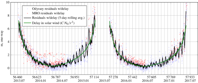
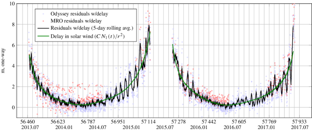
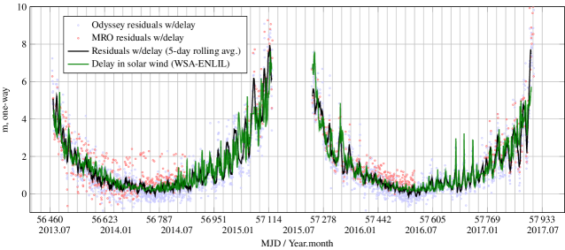
Figure 4: Odyssey and MRO range residuals without correction for delay in solar wind (blue and red points, respectively), their 5-day rolling averages (black curve), and model values (green curve) of delays in solar wind fitted to observations via the factor $C$. The top plot corresponds to Solution I ($CN_{0}/r^{2}$ model), the middle plot corresponds to Solution II ($CN_{1}(t)/r^{2}$ model), and the bottom plot corresponds to Solution III (WSA-ENLIL model). The time span is from mid-2013 to mid-2017. The vertical grid lines are placed 27.2753 days apart so as to assist in examining the periodic variations due to the Sun’s rotation.

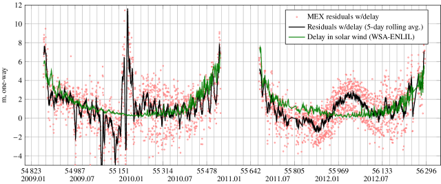
Figure 5: MEX range residuals without correction for delay in solar wind (red points) their 5-day rolling averages (black curve), and model values (green curve) of solar wind delays fitted to observations via the factor $C$. The plot corresponds to Solution III (WSA-ENLIL model). The time span is from mid-2013 to mid-2017. The vertical grid lines are placed 27.2753 days apart so as to assist in examining the periodic variations due to the Sun’s rotation.

The statistics of the postfit results and values of important parameters are given in Table 2. Solution II (time-dependent symmetric model) is slightly better than Solution I (stationary symmetric model) overall by the reduced $\chi^{2}$ metric and particularly better near conjunctions. Solution III (WSA-ENLIL-based solar wind delay model) is no better than Solution II, most probably because of the aforementioned problems with magnetograms.

Table 2: Weighted root-mean-square (WRMS) statistics and values of important parameters in the three solutions. The listed uncertainties are $3\sigma$.

	Solution I	Solution II	Solution III
	$1/r^{2}$	$1/r^{2}$ + OMNI	WSA-ENLIL
WRMS
Odyssey	0.564 m	0.563 m	0.563 m
— conj.†	1.16 m	1.15 m	1.15 m
MRO	0.619 m	0.620 m	0.619 m
	1.20 m	1.19 m	1.19 m
MEX	2.46 m	2.46 m	2.46 m
	1.96 m	1.96 m	1.95 m
VEX	6.24 m	6.04 m	6.04 m
Density	$1.31\pm 0.81$	$1.037\pm 0.03$	$1.037\pm 0.03$
factor $C$
$\Delta GM_{\odot}^{\ddagger},\ \mathrm{km}^{3}/\mathrm{s}^{2}$	$0.972\pm 0.526$	$1.457\pm 0.463$	$1.470\pm 0.463$
Variance of	1.1127	1.1124	1.1124
unit weight
(reduced $\chi^{2}$)
† “conj.” (conjunction) observations are those where the closest distance from the Earth–Mars signal to the Sun is between 30 and 60 solar radii
‡ $\Delta GM_{\odot}=GM_{\odot}-132712440041\ \mathrm{km}^{3}/\mathrm{s}^{2}$

In Solutions II and III, the electron density delay factor $C$ was constrained by Tikhonov regularization to be close to the reference value of 1. An additional experiment (not shown) was made where the Tikhonov regularization was not applied to $C$ in Solution II. The resulting value of $C$ turned out to be $1.35\pm 0.81$ (as opposed to $1.037\pm 0.03$ in ordinary Solution II). This confirms that proper usage of absolute in situ measurements of electron density really helps to bring the solution, including the $GM_{\odot}$ estimate, closer to reality. Also, the constraint on the factor helps to reduce the uncertainty of $GM_{\odot}$ by $\sim 12$% (the uncertainty is 0.526 in Solution I and 0.463 in Solution II).

Another important improvement of Solution II over previous EPM solutions is that only a single parameter related to solar wind is fit in the solution, as compared to more than 50 in EPM2017 (see $B$ and $\dot{B}$ in eq. 1, per-year, per-planet) or 10 ($B$ per-conjunction from 2002 to 2018 and single $B$ prior to 2002) in a later EPM version that was not released (Pavlov, 2019; Pitjeva et al., 2021).

6 Conclusion and future work

Conclusion:

• Interplanetary spacecraft ranging observations are sensitive to signal delay due to solar wind and, in particular, to its medium-term variations caused by the rotation of the Sun, and to its long-term variations caused by changes in Sun’s activity.

• The ENLIL model of solar wind, built on daily magnetograms done by the GONG network, can serve as a basis for a numerical solar wind delay model. Such a model, though, can have or not have a good match to the MRO and Odyssey ranges. Spacecraft ranges that pass through the parts of the electron density map that are effectively built from visible disk magnetograms have (with otherwise equal conditions) better residuals than the ranges that pass through the parts of the map that are built from older magnetograms rotated to the present date.

• Mathematical model of ephemeris can benefit from taking into account a solar wind delay model that has long-term variability determined from the OMNI dataset of in situ observations.

• Constraining the (usually unconstrained) electron density factor in a planetary ephemeris solution to a reasonable range allows to reduce the error in the determined gravitational parameter of the Sun by $\sim$ 12%.

• Using the WSA-ENLIL-based solar wind delay model to account for medium-term variations can improve the residuals in individual cases, but does not improve the solution overall.

Interplanetary spacecraft ranging observations are sensitive enough to electron density so that they are used in this work to perform comparative analysis and validation of solar wind models. They can be used for validation of future solar wind models; and potentially they can be used as a source of data for solar wind models.

Data Availability

The Mars Global Surveyor (MGS), Mars Reconnaissance Orbiter (MRO), and Odyssey spacecraft ranging data underlying this article are available at the webpage of Solar System Dynamics (SSD) group at NASA JPL.

The extended set of ranges for MRO and Odyssey up to the end of 2017 was kindly provided by William Folkner of the SSD group by permission and may be shared on reasonable request to the SSD team of NASA JPL.

Mars Express (MEX) and Venus Express (VEX) ranges were downloaded from the Geoazur website.

The WSA-ENLIL data were produced by request via the “Runs on Request” service at the Community Coordinated Modeling Center (CCMC) website. The data are available for download through the “Runs on Request” service, the names of the runs are:

• Dan_Aksim_122319_SH_2 (2006)

• Dan_Aksim_122319_SH_3 (2007)

• Dan_Aksim_122319_SH_4 (2008)

• Dan_Aksim_122319_SH_5 (2009)

• Dan_Aksim_122319_SH_6 (2010)

• Dan_Aksim_122319_SH_7 (2011)

• Dan_Aksim_122319_SH_8 (2012)

• Dan_Aksim_122319_SH_9 (2013)

• Dan_Aksim_120920_SH_1 (2014)

• Dan_Aksim_122319_SH_11 (2015)

• Dan_Aksim_122319_SH_12 (2016)

• Dan_Aksim_112119_SH_3 (2017)

The OMNI in situ data are available publicly through the OMNIWeb website. Specifically, the file “omni_01_av.dat”, containing daily averages of solar wind parameters, comes from the low-resolution version of the OMNI dataset.

Appendix A Radio ranging residuals and determination of parameters

Radio signal travels twice the distance between the observatory on Earth and the spacecraft. The time delay is being measured. The ranging residual is the difference between the “observed” delay (normal point, see Sec. 3.1) and the model (“computed”) value of the delay. The process of calculation of “observed minus computed” value of the delay is called reduction.

The precision of the normal point is sub-meter; for the model value to match that precision, its formula must account for: the speed of light, relativistic signal delay caused by Sun and other massive bodies, proper time of observer, delay in troposphere and ionosphere, delay in solar wind. All the mentioned delays are to be calculated twice — for the up and down legs of the signal. A detailed description can be found e.g. in Moyer (2003). For each normal point, two equations are solved iteratively: one to find the time of retransmission of signal by the spacecraft; and the other to find the time of reception of the retransmitted signal.

Observations must also be corrected for the spacecraft transponder delay (the short moment of time between reception of signal by the spacecraft and transmission of the return signal). There is always some delay; it is measured before launch, but varies due to space conditions as the spacecraft makes its way to the planet. The transponder delay thus itself must be determined from radio ranges.

In addition to transponder delays, there are biases that come from miscalibrations on radio observatories. Following the decision from Kuchynka et al. (2012), two sets of biases were determined for Deep Space Network (DSN) stations: one for MGS and Odyssey spacecraft, another for the MRO spacecraft.

In short, the following system of equations has to be solved for each observable:

$$\begin{cases}t_{2}-t_{1}=\frac{|{\bm{p}}_{\mathrm{BCRS}}(t_{2})-{\bm{s}}_{\mathrm{BCRS}}(t_{1})|}{c}+\Delta_{\mathrm{grav}}(t_{1},t_{2})+\Delta_{\mathrm{atm}}(t_{1},t_{2})+\Delta_{\mathrm{sol}}(t_{1},t_{2}),\\ t_{3}-t_{2}=\frac{|{\bm{p}}_{\mathrm{BCRS}}(t_{3})-{\bm{s}}_{\mathrm{BCRS}}(t_{2})|}{c}+\Delta_{\mathrm{grav}}(t_{3},t_{2})+\Delta_{\mathrm{atm}}(t_{3},t_{2})+\Delta_{\mathrm{sol}}(t_{3},t_{2}),\end{cases}$$ (5)

where $t_{1}$, $t_{2}$, and $t_{3}$ are the times of emission, reflection, and reception of the signal in the Barycentric Dynamical Time (TDB), a timescale that represents time at the barycenter of the Solar system. Usually, a normal point contains $t_{1}$ in UTC, and conversion to TDB is required. ${\bm{p}}_{\mathrm{BCRS}}$ and ${\bm{s}}_{\mathrm{BCRS}}$ are the positions of the center of the planet and the reference point of the radio observatory (station) in the barycentric celestial reference system (BCRS).

The “computed” value of the delay is

$$C=c\left[t_{3}-t_{1}\vphantom{x^{x}}\right.+ \ \textrm{[TT}-\textrm{TDB]}(t_{3},{\bm{s}}_{\mathrm{BCRS}}(t_{3}))\ -$$ (6)

$$\left.\vphantom{x^{x}}\textrm{[TT}-\textrm{TDB]}(t_{1},{\bm{s}}_{\mathrm{BCRS}}(t_{1}))\right]+b,$$

where $b$ is the sum of transponder delay and the bias (converted to units of distance). TT stands for terrestrial time—a timescale based on atomic clock and representing time on Earth’s surface. For calculating $[\textrm{TT}-\textrm{TDB}]$ at time $t$ and point ${\bm{s}}_{\mathrm{BCRS}}(t)$, a theoretical equation is used, which can be found for instance in (Moyer, 2003, eq. 2-23). The geocentric terms of the equation are integrated along with the Solar system equations and stored in ephemeris; just one topocentric term is taken into account in Equation 6: $\left(\bm{\dot{r}}_{E}(t)\cdot({\bm{s}}_{\mathrm{BCRS}}(t)-\bm{r}_{\mathrm{E}}(t))\right)/c^{2}$.

One has to transform the position of the station in the terrestrial reference frame to geocentric celestial reference frame (GCRS) at times $t_{1}$ and $t_{3}$. The standard IAU2000/2006 precession-nutation model (Wallace & Capitaine, 2006) and IERS EOP series (Bizouard et al., 2011) are used for this. Also, displacements of the station due to solid Earth tides and pole tides are to be calculated according to the IERS Conventions 2010 (Petit & Luzum, 2010).

$\Delta_{\mathrm{grav}}$ is the delay of the signal due to spacetime curvature; it was calculated in this work with a theoretical approximation (Kopeikin, 1990); delays from the Sun, Earth, the Moon, Jupiter, and Saturn were added up.

$\Delta_{\mathrm{atm}}$ is the delay of the signal in ionosphere and troposphere, usually calculated according to respective IERS models (Petit & Luzum, 2010). In this work, the given observations (normal points) were already corrected for the atmospheric delay.

$\Delta_{\mathrm{sol}}$ is the delay of the signal in solar wind, the subject of this work.

While the “observed” values are known and do not change, the “computed” values depend on model parameters (see Section 4.1). The model parameters are to be fitted so that the differences between the observed and computed, i.e. residuals, are minimized. The values of residuals obtained after the fitting (minimization) are called postfit residuals.

The fitting is done via the Gauss–Newton method. The following function is subject to minimization over $\bm{\beta}$:

$$S({\bm{\beta}})=\sum_{i=1}^{m}\frac{r_{i}({\bm{\beta}})^{2}}{\sigma_{i}^{2}}+\sum_{j=1}^{n}\frac{(\beta_{j}-\mu_{j})^{2}}{\varepsilon_{j}^{2}},$$ (7)

where $\bm{\beta}$ is the vector of all model parameters, $r_{i}$ is the $i$-th residual ($m$ being the number of observations), and $\sigma_{i}$ is the a priori error (formal error) that represents the standard deviation of the noise of the $i$-th observation.

In reality, the “true” thermal noise of measurement is hard to separate from other systematic errors unaccounted for in the model. The main source of those errors is the solar wind plasma itself; also there can be errors from incompleteness of the set of perturbing asteroids (see sec. 4.2) or from wrong estimates of asteroid masses or orbits. Finally, systematic errors (other than the aforementioned constant offsets) can come from hardware on the spacecraft or at the radio observatory. A frequent approach to overcome this problem, which is also used in this work, is to choose the formal errors to be somewhat smaller than a posteriori estimates of the standard deviation of noise. Those estimates come from postfit residuals (see Sec. 5). The decision to make the formal errors smaller than the postfit residuals was made in order to account for systematic errors in processing otherwise unaccounted for.

The second term of eq. 7 comes from the Tikhonov regularization modification of least-squares. $\mu_{j}$ is the a priori value of the parameter $\beta_{j}$, while $\varepsilon_{j}$ is the prior uncertainty of that value (taking $\varepsilon_{j}=\infty$ will mean effectively no prior value).

Appendix B Difficulties of determination of solar wind model parameters simultaneously with other parameters of planetary ephemeris solution

Apart from solar wind plasma delay, observations of radio signal delays always contain unknowns that are not directly related to solar wind, but have a similar effect on the ranges. It is important not to be overly confident in e.g. the determined value of the power $\epsilon$ in the $1/r^{\epsilon}$ model of solar wind density. Figure 6 provides a synthetic example with $\epsilon=2.5$. Let us assume that the “real” solar wind behaves according to the $1/r^{2}$ model, but we fit the $1/r^{2.5}$ model to observations. That is, we must fit the electron density factor, but also an offset (bias) that is inherent to spacecraft observations. It turns out that the $1/r^{2.5}$ model can be made virtually equivalent to the $1/r^{2}$ one as long as a factor and a bias are fitted, and signal paths that pass closer than 15 solar radii to the Sun are excluded from the analysis due to their bad quality, as they normally are in ephemeris solutions (in fact, the barrier is often 30 solar radii or more).

Another example concerns the fitted electron density factor itself. Even if the power of $r$ in the model is correct, it is important not to be overly confident in the determined factor. In a planetary ephemeris solution, the $GM_{\odot}$ is an unknown parameter that has to be determined from observations. In EPM, the $GM_{\odot}$ is not routinely determined directly; a distance scale parameter is determined instead. In any case, an incorrect value of the $GM_{\odot}$ adds an error to the computed range, proportional to the range itself. The delay of radio signal in solar wind is largest near Sun–Mars conjunctions; it so happens that the Earth–Mars distance follows the same pattern. That, together with the unknown bias that also has to be fitted, makes the two sources of error not perfectly separable, as illustrated by a synthetic example on Figure 7. Let us assume that the blue curve is the “real” delay in solar wind. If no reduction for solar wind delay was made in the residuals, the residuals will lie on the blue curve. But if, instead of taking into account the solar wind delay, we decide to fit the distance scale factor and bias, we will end up subtracting the red curve from the residuals. The blue curve is not very far off from the blue curve. This leads to the conclusion that an incorrectly determined value of the electron density factor can be partially absorbed by a small scale factor (and hence a small change in the mass of the Sun) and small offset.

Figure 6: Earth–Mars signal delays with $1/r^{2}$ and $1/r^{2.5}$ density models. The multiplier (0.37) and the additive constant (1.16 m) for the $1/r^{2.5}$ curve are chosen so that the curve fits the $1/r^{2}$ curve on 57974–58119 interval, which corresponds to Earth–Mars signal passing farther than $15R_{\odot}$ from the Sun.

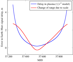
Figure 7: Red curve (change of Earth–Mars range due to scale) fitted to the blue curve (model values of delay in solar wind), with a factor of ($1+9.67\times 10^{-12}$) and an offset of 0.97 m. The two curves are correlated at 87%.

References

- Aksim et al. (2019) Aksim D., Melnikov A., Pavlov D., Kurdubov S., 2019, The Astrophysical Journal, 885, 159
- Arge & Pizzo (2000) Arge C. N., Pizzo V. J., 2000, Journal of Geophysical Research: Space Physics, 105, 10465
- Bizouard et al. (2011) Bizouard C., Lambert S., Becker O., Richard J. Y., 2011, Preliminary draft, The combined solution C04 for Earth Rotation Parameters consistent with International Terrestrial Reference Frame 2014. Observatoire de Paris, SYRTE, http://hpiers.obspm.fr/iers/eop/eopc04/C04.guide.pdf
- Bougeret et al. (1984) Bougeret J.-L., King J., Schwenn R., 1984, Solar Physics, 90
- Callahan (1977) Callahan P. S., 1977, The Deep Space Network progress report 42-39, A preliminary analysis of Viking S-X Doppler data and comparison to results of Mariner 6, 7, and 9 DRVID measurements of the solar wind turbulence. NASA JPL, https://ipnpr.jpl.nasa.gov/progress_report2/42-39/39E.PDF
- Folkner et al. (2014) Folkner W., Williams J., Boggs D., Park R., Kuchynka P., 2014, IPN Progress Report 42-196, The Planetary and Lunar Ephemerides DE430 and DE431. NASA JPL, http://naif.jpl.nasa.gov/pub/naif/generic_kernels/spk/planets/de430_and_de431.pdf
- Hill (2018) Hill F., 2018, Space Weather, 16, 1488
- Hovestadt et al. (1995) Hovestadt D., et al., 1995, Solar Physics, 162, 441
- Kahaner et al. (1989) Kahaner D., Moler C., Nash S., 1989, Numerical methods and software. Prentice-Hall, Inc.
- Kan & Pavlov (2022) Kan M., Pavlov D., 2022, in Astronomy at the Epoch of Multimessenger Studies. Proceedings of the VAK-2021 Conference, Aug 23–28, 2021. SAI MSU, INASAN, pp 93–95, https://www.vak2021.ru/wp-content/uploads/2022/03/VAK_2021_proceedings.pdf
- King & Papitashvili (2005) King J. H., Papitashvili N. E., 2005, Journal of Geophysical Research: Space Physics, 110, A02104
- Kopeikin (1990) Kopeikin S. M., 1990, Sov. Astron., 34, 5
- Kuchynka & Folkner (2013) Kuchynka P., Folkner W. M., 2013, Icarus, 222, 243
- Kuchynka et al. (2010) Kuchynka P., Laskar J., Fienga A., Manche H., 2010, Astronomy and Astrophysics, 514, A96
- Kuchynka et al. (2012) Kuchynka P., Folkner W. M., Konopliv A. S., 2012, Interplanetary network progress report 42-190, Station-Specific Errors in Mars Ranging Measurements. NASA JPL, https://ipnpr.jpl.nasa.gov/progress_report/42-190/190C.pdf
- Leblanc et al. (1998) Leblanc Y., Dulk G. A., Bougeret J.-L., 1998, Solar Physics, 183, 165
- Mann et al. (1999) Mann G., Jansen F., MacDowall R. J., Kaiser M. L., Stone R. G., 1999, Astronomy and Astrophysics, 348, 614
- Masiero et al. (2011) Masiero J. R., et al., 2011, The Astrophysical Journal, 741, 68
- Mays et al. (2020) Mays M. L., et al., 2020, Technical report, NASA/NOAA MOU Annex Final Report: Evaluating Model Advancements for Predicting CME Arrival Time. CCMC, https://ccmc.gsfc.nasa.gov/annex/files/CCMC_SWPC_annex_final_report.pdf
- Morley & Budnik (2009) Morley T., Budnik F., 2009, in 21st International Symposium on Space Flight Dynamic. http://issfd.org/ISSFD_2009/OrbitDeterminationI/Morley.pdf
- Moyer (2003) Moyer T. D., 2003, Formulation for Observed and Computed Values of Deep Space Network Data Types for Navigation. Wiley
- Muhleman & Anderson (1981) Muhleman D. O., Anderson J. D., 1981, ApJ, 247, 1093
- Odstrcil (2003) Odstrcil D., 2003, Advances in Space Research, 32, 497
- Odstrcil (2004) Odstrcil D., 2004, Technical report, ENLIL: A Numerical Code for Solar Wind Simulations. CCMC, https://ccmc.gsfc.nasa.gov/models/Code_description.pdf
- Papitashvili et al. (2014) Papitashvili N., Bilitza D., King J., 2014, in 40th COSPAR Scientific Assembly. pp C0.1–12–14
- Park et al. (2017) Park R. S., Folkner W. M., Konopliv A. S., Williams J. G., Smith D. E., Zuber M. T., 2017, The Astronomical Journal, 153
- Patzold et al. (2004) Patzold M., et al., 2004, SP-1240, MaRS: Mars Express Orbiter Radio Science. European Space Agency, https://sci.esa.int/documents/33745/35957/1567254725449-PatzoldWeb.pdf
- Pavlov (2019) Pavlov D., 2019, Journal of Geodesy, 94
- Pavlov & Skripnichenko (2015) Pavlov D., Skripnichenko V., 2015, in Malkin Z., Capitaine N., eds, Proceedings of the Journées 2014 “Systèmes de référence spatio-temporels”. Pulkovo Observatory, pp 243–246, https://syrte.obspm.fr/jsr/journees2014/pdf/Pavlov.pdf
- Pavlov et al. (2016) Pavlov D., Williams J., Suvorkin V., 2016, Celestial Mechanics and Dynamical Astronomy, 126(1), 61
- Petit & Luzum (2010) Petit G., Luzum B., 2010, IERS Conventions 2010 (IERS Technical Note 36). Verlag des Bundesamts für Kartographie und Geodäsie, Frankfurt am Main
- Pitjeva (2004) Pitjeva E. V., 2004, Proceedings of the International Astronomical Union, pp 230–241
- Pitjeva (2013) Pitjeva E. V., 2013, Solar System Research, 47, 386
- Pitjeva & Pavlov (2017) Pitjeva E. V., Pavlov D. A., 2017, Technical report, EPM2017 and EPM2017H. Institute of Applied Astronomy RAS, http://iaaras.ru/en/dept/ephemeris/epm/2017
- Pitjeva & Pitjev (2014) Pitjeva E. V., Pitjev N. P., 2014, Celestial Mechanics and Dynamical Astronomy, 119, 237
- Pitjeva & Pitjev (2018a) Pitjeva E. V., Pitjev N. P., 2018a, Astronomy Letters, 44, 554
- Pitjeva & Pitjev (2018b) Pitjeva E. V., Pitjev N. P., 2018b, Celestial Mechanics and Dynamical Astronomy, 130, 57
- Pitjeva et al. (2021) Pitjeva E. V., Pitjev N. P., Pavlov D. A., Turygin C. C., 2021, A&A, 647, A141
- Remus et al. (2014) Remus S., Hahn M., Bird M., Paetzold M., Haeusler B., Asmar S., Witasse O., Tyler G., 2014, Issue 2, Revision 1, Solar Corona Experiment: A Cookbook. European Space Agency, https://www.cosmos.esa.int/documents/772136/977578/Solar_Corona_Experiment___A_Cookbook_17Mar2014.pdf
- Savitzky & Golay (1964) Savitzky A., Golay M. J. E., 1964, Analytical Chemistry, 36, 1627
- Sheeley Jr (2017) Sheeley Jr N. R., 2017, History of Geo-and Space Sciences, 8, 21
- Shishov et al. (2016) Shishov V. I., et al., 2016, Astronomy Reports, 60, 1067
- Standish (1990) Standish E. M. J., 1990, Astronomy and Astrophysics, 233, 252
- Stone et al. (1998) Stone E., Frandsen A., Mewaldt R., Christian E., Margolies D., Ormes J., Snow F., 1998, Space Science Reviews, 86, 1
- Tedesco et al. (2004) Tedesco E. F., Noah P. V., Noah M., Price S. D., 2004, Technical report, IRAS Minor Planet Survey V6.0. NASA Planetary Data System
- Thompson (2006) Thompson W. T., 2006, Astronomy & Astrophysics, 449, 791
- Verma et al. (2013) Verma A. K., Fienga, A. Laskar, J. Issautier, K. Manche, H. Gastineau, M. 2013, A&A, 550, A124
- Wallace & Capitaine (2006) Wallace P. T., Capitaine N., 2006, A&A, 459, 981
- Wang & Sheeley Jr (1990) Wang Y.-M., Sheeley Jr N., 1990, The Astrophysical Journal, 355, 726
- Wilson III et al. (2021) Wilson III L. B., et al., 2021, Reviews of Geophysics, 59