A Systematic Look at the Temperature Gradient Contribution to the Dayside Magnetopause Current

Abstract

Magnetopause diamagnetic currents arise from density and temperature driven pressure gradients across the boundary layer. While theoretically recognized, the temperature contributions to the magnetopause current system have not yet been systematically studied. To bridge this gap, we used a database of Magnetospheric Multiscale (MMS) magnetopause crossings to analyze diamagnetic current densities and their contributions across the dayside and flank magnetopause. Our results indicate that the ion temperature gradient component makes up to 37% of the ion diamagnetic current density along the magnetopause and typically opposes the classical Chapman-Ferraro current direction, interfering destructively with the density gradient component, thus lowering the total diamagnetic current density. This effect is most pronounced on the flank magnetopause. The electron diamagnetic current was found to be 5 to 14 times weaker than the ion diamagnetic current on average.

Geophysical Research Letters

Department of Physics, The Catholic University of America, Washington D.C. USA NASA Goddard Space Flight Center, Greenbelt, MD, USA Space Sciences Laboratory, University of California, Berkeley, CA, USA

Jason Beedlebeedle@cua.edu

The magnetopause diamagnetic current is composed of opposing density and temperature gradient generated components

The temperature gradient contributes up to 37% of the ion diamagnetic current density along the magnetopause

The temperature component typically opposes the classical Chapman-Ferraro current direction

Plain Language Summary

The solar wind represents a continuous outflow of charged particles from the Sun’s upper atmosphere into the solar system. Upon reaching Earth’s magnetosphere, the solar wind’s dynamic pressure is balanced by the magnetic pressure of Earth’s magnetic field in a boundary layer known as the magnetopause. This boundary layer represents the entry point of the solar wind’s energy into Earth’s magnetosphere and upper atmosphere, playing a crucial role in energy transport throughout the interconnected system. Plasma density and temperature differences across the boundary layer generate an electric current that supports the magnetopause. In this paper, we clarify the physical mechanism of the magnetopause current by using high-resolution data from NASA’s MMS mission. We found a significant ion temperature contribution to the magnetopause current not identified in previous studies. Our results also indicated that the plasma electrons’ contribution to the magnetopause current was significantly smaller than the ion contribution.

1 Introduction

The magnetopause is a magnetosphere boundary layer created through the dynamic pressure balance between the solar wind’s kinetic pressure and Earth’s magnetic field. The solar wind causes distortions in the magnetosphere’s magnetic field topology supported by a current sheet first proposed by Chapman and Ferraro in 1931 [Chapman  Ferraro (1931)], often termed the Chapman-Ferraro (CF) current, which runs in a dawn-to-dusk direction around the magnetopause [Ganushkina . (2018)]. This current structure is believed to be generated through pressure gradients at the magnetopause boundary layer where, as explained in Hasegawa2012, the magnetosheath plasma has a higher plasma density, while the magnetosphere will have a higher ion temperature. The resulting changes in plasma density and temperature across the magnetopause leads to gradients that generate ion and electron diamagnetic currents running perpendicular to the magnetic field [Ganushkina . (2018)].

Because of the magnetopause’s important role in magnetic reconnection and the resulting transfer of plasma and energy into the magnetosphere it has been the focus of numerous studies [Cahill1963; Le1994; PhanLarson1996; PhanPaschmann1996; Haaland2014; Paschmann2018; Haaland2019; Shuster2019; Haaland2020; etc.] and missions [MMS, THEMIS, and Cluster] which have delved deeper into the current sheet’s structure and creation. From Paschmann2018 and their MMS magnetopause crossing database, the total current density across the dayside magnetopause was studied in detail. The flank magnetopause total current density was then surveyed in Haaland2019 and Haaland2020 where the flanks were found to have a weaker current density and a correspondingly thicker boundary layer than the dayside.

While the literature generally recognizes the importance of both the density and temperature in generating diamagnetic currents, a large scale systematic analysis of their contribution to the magnetopause current system has not yet been accomplished. To help fill this gap in the literature, we considered four years of burst mode MMS mission data over the magnetopause crossing intervals provided by Paschmann2018’s MMS database. We measured both the density and temperature diamagnetic current components and created current accumulations of their contributions. In doing so, we found that the temperature diamagnetic current component is a statistically significant factor to both the dayside and flank magnetopause current sheet by acting against the density component and thus reducing the total diamagnetic current density.

2 Data and Analysis

2.1 MMS Database

For this study, we used four years of data from Paschmann2018,Paschmann2020’s and Haaland2020’s database of MMS current sheet crossings. MMS is a mission comprised of four separate spacecraft traveling in a tetrahedron pattern through the magnetopause [Burch . (2015)]. This database catalogues MMS current sheet crossings based on Fast Plasma Investigation (FPI) [Pollock . (2016)], Fluxgate Magnetometer [Russell . (2016)], and Hot Plasma Composition Analyzer (HPCA) measurements [Young . (2016)]. The magnetopause transit times are captured through an automated minimum variance analysis (MVA) of the magnetic field in boundary normal or LMN coordinates [Paschmann . (2018), Paschmann . (2020)]. The start and end times of the current sheet crossing were then assigned as covering 76% of the primary magnetic field component’s ($B_{L}$’s) transition across the magnetopause boundary, which represents the thickness of a tanh fit of the $B_{L}$ profile.

The magnetopause velocities for each crossing are obtained through a de Hoffman-Teller analysis and stored by the database as the de Hoffman-Teller velocity ($V_{HT}$). We then took these velocities and dotted them with the normal direction in the LMN coordinate system to get the normal magnetopause boundary velocity ($V_{n}$) [Sonnerup  Scheible (1998), Khrabrov  Sonnerup (1998a), Paschmann . (2018)]. The magnetopause thicknesses are then determined by taking this normal velocity and multiplying it by the time span of the current sheet as determined by the MVA analysis.

The database places identifiers on the individually identified magnetopause crossings, classifying their characteristics and structure. A full description of this process and the current sheet identifiers can be found in Paschmann2018 and Haaland2020. An example crossing, with the database defined magnetopause current sheet crossing indicated by the dashed orange lines, is given in Figure 1.

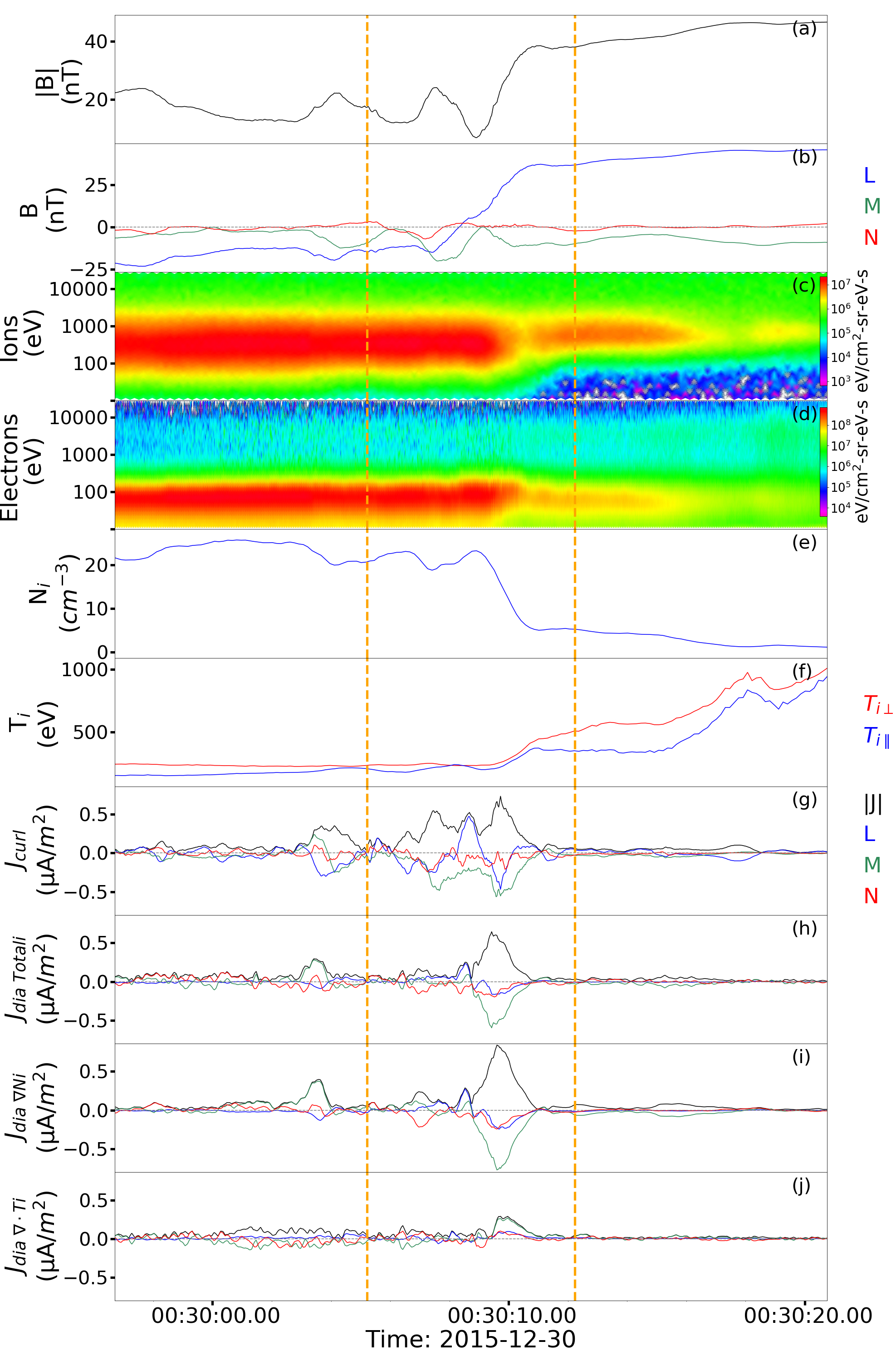
Figure 1: Example crossing during a monotonic (constant magnetopause velocity), complete 2015 MMS transit from the magnetosheath into the magnetosphere at the following Cartesian GSE position along the dayside magnetopause, indicated in Earth Radii (X,Y,Z): (9.4 Re, -6.5 Re, -1.0 Re). The orange lines represent the magnetopause current sheet as identified by the MMS database. (a) Magnitude of the magnetic field, (b) magnetic field in LMN coordinates, (c,d) ion and electron omnidirectional spectrograms, (e) ion number density, (f) ion perpendicular and parallel temperature, and (g,h,i,j) curlometer, total ion diamagnetic, density component, and temperature component current densities respectively in LMN coordinates with magnitudes indicated in black.

2.2 Magnetopause Current Sheet Selection

We chose database defined crossings from 2015 to 2018 using event identifiers to select for complete and monotonic magnetopause crossings, where monotonic indicated events that had a constant magnetopause velocity so their thicknesses and durations could be computed. Additionally, we included Harris sheet-like events, or simple clear magnetopause crossings that were also complete, monotonic events in our data set. Events with unusually high (above $2,000$ $nA/m^{2}$) current density spikes during the magnetopause crossing time, such as would occur during a reconnection event, or when data flags for the various instruments were non-nominal, were manually removed from our data set.

Alongside the database defined event criteria, we imposed two additional conditions on our events in order to ensure high signal-to-noise ratios and typical magnetopause plasma number densities as described below:

First, we considered the current measured during the magnetopause crossing and selected for events that reported significant peaks in their current densities. Where “significant” in our case was considered to be a current crossing where at least 50% of the crossing duration was within 15% of the maximum current peak during that crossing. This condition enabled us to select events with a strong current and high signal-to-noise ratios, thus ensuring that the temperature and density gradients and their resulting diamagnetic current components were not artificially diminished by the higher noise floor of low current density magnetopause crossings.

Second, we used HPCA measurements to compare the number densities of $H^{+}$ with $O^{+}$ for each magnetopause crossing. If $O^{+}$ exceeded $0.2$ $cm^{-3}$ during the transit and $H^{+}$ remained below $1.5$ $cm^{-3}$, then we considered $O^{+}$ to dominate the magnetospheric ion mass density by more than a factor of 2 as described by Fuselier2019. Events fitting this classification were also removed from our data set as they represented densities not typically found in the magnetopause current sheet.

From the application of the database identifiers as well as our conditions, we were able to identify 561 events. The locations and corresponding years of the selected crossings are denoted in Figure 2.

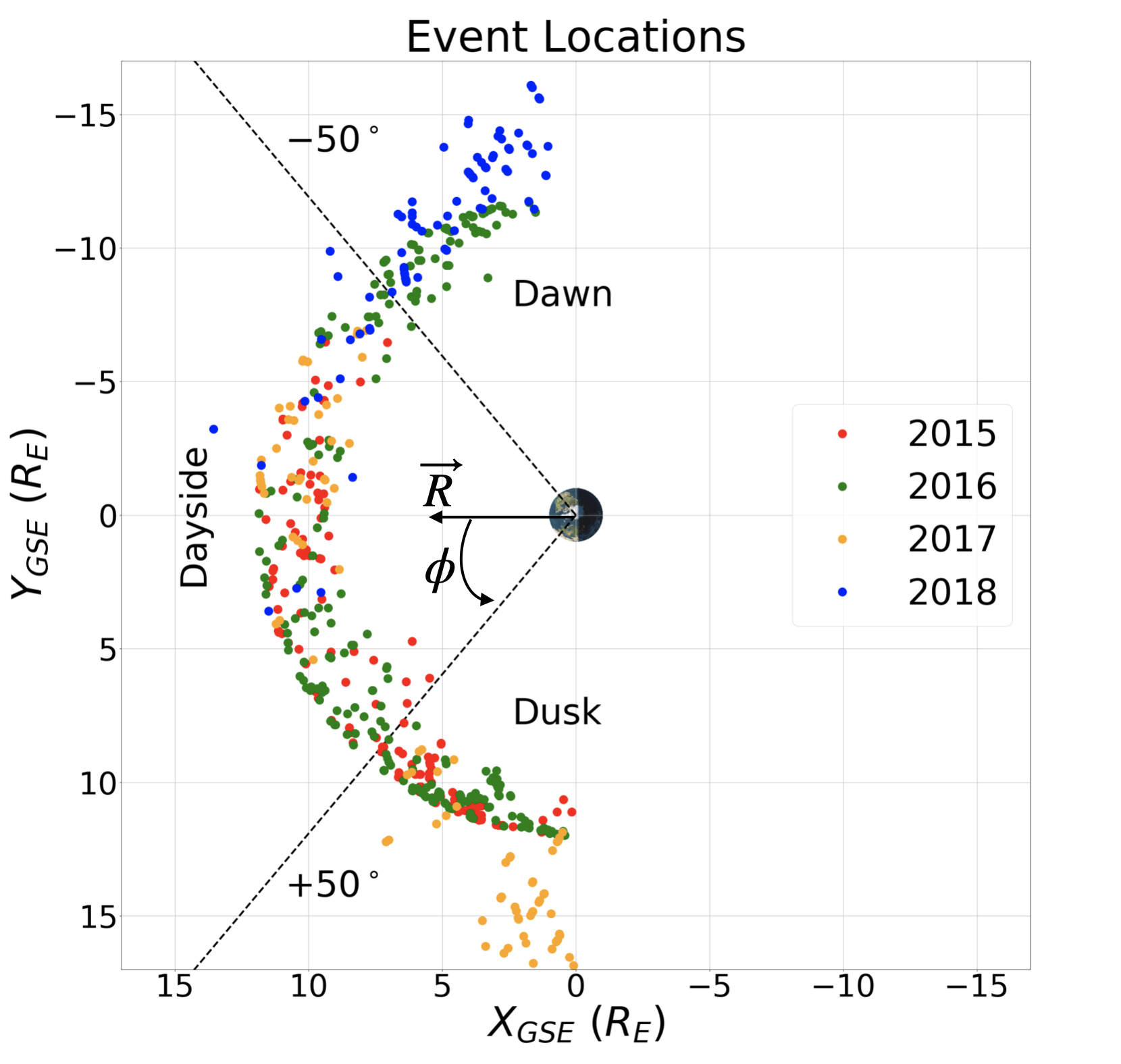
Figure 2: Diagram of our 561 MMS magnetopause crossings from 2015 (red), 2016 (green), 2017 (orange), and 2018 (blue). We define a local spherical coordinate system with $\phi$ in the $X_{GSE}$ - $Y_{GSE}$ plane, positively defined from the $+X_{GSE}$ axis, R defined as radially outward, and $\theta$ as the polar angle into the $Z_{GSE}$ direction. Note, every $15^{\circ}$ in $\phi$ is equal to 1 hour of MLT with 12 MLT corresponding to $0^{\circ}$ in $\phi$, or along the +$X_{GSE}$ axis. The Dawn flank is defined as $-50^{\circ}$ to $-90^{\circ}$ in $\phi$, the Dusk flank as $+50^{\circ}$ to $+90^{\circ}$, and the Dayside as $+50^{\circ}$ to $-50^{\circ}$. Note, MMS first launched in 2015 with an orbit focusing on the dayside magnetopause, but after 2017, this orbit was extended to a wider orbit focusing on the flank magnetopause [Haaland . (2020)]. Because of the varying solar cycle, this has the possibility of creating an asymmetry between the dawn and dusk flank plasma measurements.

2.3 Current Calculations

MMS’s four separate spacecraft allows the total current to be calculated by the curlometer method [Dunlop . (1988)] that uses all four spacecraft to perform the curl of the observed magnetic field in order to approximate Ampere’s law in the MHD approximation (e.g. Ganushkina2017). This current we call the curlometer current:

$$\textbf{J}_{curl}=\frac{\nabla\times\textbf{B}}{\mu_{0}}.$$ (1)

Using the curlometer method, we also calculated the gradient of the ion density, and the divergence of the temperature tensor to get the total ion diamagnetic current and its current components ($\textbf{J}_{dia\ \nabla N_{i}}$ and $\textbf{J}_{dia\ \nabla\cdot\overleftrightarrow{T_{i}}}$ ). We found the electron diamagnetic current to be at least one order of magnitude smaller, on average, than the ion diamagnetic current. This is in agreement with the results of Dong2018 in their case study where they found that the ion diamagnetic current was the primary source of perpendicular current in the magnetopause. Thus we are presenting results for the ion components and will drop the signifier “i” going forward. The components of the total diamagnetic current are found by imputing the ideal gas law, $\overleftrightarrow{P}=Nk_{b}\overleftrightarrow{T}$, into the expression for the total diamagnetic current $J_{\perp}=\frac{\vec{B}\times\nabla\cdot\overleftrightarrow{P}}{|B|^{2}}$, see e.g. Ganushkina2017 and the references therein, resulting in the following expressions:

$$\textbf{J}_{dia\ \nabla N}=\frac{\textbf{B}\times(K_{b}\overleftrightarrow{T}\cdot\nabla N)}{|\textbf{B}|^{2}}\ \ ,\ \ \textbf{J}_{dia\ \nabla\cdot\overleftrightarrow{T}}=\frac{\textbf{B}\times(K_{b}N\nabla\cdot\overleftrightarrow{T})}{|\textbf{B}|^{2}}.$$ (2)

Where, by definition, $\textbf{J}_{dia\ Total}=\textbf{J}_{dia\ \nabla N}+\textbf{J}_{dia\ \nabla\cdot\overleftrightarrow{T}}$.

These currents were then averaged over our selected magnetopause crossings for each event, leading to single averaged current values for each of our 561 crossings. See Figure 1 for an example crossing on the dayside magnetopause. Note the two vertical orange lines represent the database defined current sheet crossing where the resulting currents would be averaged over.

All of the data taken from MMS, as well as the current calculations, was interpolated to the 30 ms FPI electron time resolution. As our main results involve ion diamagnetic currents and the total current as computed from the curlometer method, any sub 150 ms variations in the ion measurements will not impact our results. For non-curlometer calculations, we averaged over all four spacecraft to create a single data stream where, on average, the MMS separation during 2015 - 2018 was 10 - 60 km while the magnetopause current crossings analyzed typically had thicknesses greater than several hundred km, sufficiently larger than the max 60 km tetrahedron separation. These calculations were completed in GSE coordinates and then converted to a local spherical coordinate system built off of the Cartesian GSE coordinates. See Figure 2 for a depiction of our spherical coordinate system and the definition of the dusk and dawn sectors.

Note, one limitation with applying the curlometer method to a magnetopause current sheet crossing is that the curlometer method requires simultaneous measurements from all four spacecraft to calculate a gradient, curl, or divergence of a quantity. Thus, errors occur when one or more of the MMS constellation is outside of the magnetopause boundary as the spacecraft are no longer all measuring the same medium. For our study, this caveat is mitigated by the fact that the magnetopause boundary is, on average, at least one order of magnitude larger than the average MMS separation, with median magnetopause thicknesses often reported as approximating 1,000 km (e.g. Haaland2019,Haaland2020). This makes times where the curlometer method results in erroneous measurements brief and limited to the outskirts of a current sheet crossing.

2.4 Current Accumulations

The averaged currents from the 561 magnetopause crossings were put into bins corresponding to MMS’s physical location in our local spherical coordinate system. The angle $\phi$ was used to create 1-dimensional bins from $90^{\circ}$ to $-90^{\circ}$ in $20^{\circ}$ increments. This was done for each component in the spherical coordinate system as described in Figure 2 and shown in Figure 3. Error bars for each figure were computed using the standard error or $\sigma/\sqrt{N}$, with $\sigma$ the standard deviation of the values in each bin and N the number of events that fell inside that bin, with the bins visually depicted in Figure 3 (a-d) by the grey-dashed lines.

Using Figure 3 we can make several observations. The first is that the $\textbf{J}_{curl}$, $\textbf{J}_{dia\ Total}$, and $\textbf{J}_{dia\ \nabla N}$ $\phi$-component currents are all in the $+\phi$ direction across the magnetopause, or in the classical CF, dawn-to-dusk direction. However, the $\textbf{J}_{dia\ \nabla\cdot\overleftrightarrow{T}}$ $\phi$ component is consistently in the $-\phi$ direction, or from dusk-to-dawn across the magnetopause. Therefore the two components of the ion diamagnetic current, $\textbf{J}_{dia\ \nabla N}$ and $\textbf{J}_{dia\ \nabla\cdot\overleftrightarrow{T}}$, are oppositely directed across the magnetopause as can be seen in Figure 3b. The directions of these components are as expected when using the magnetospheric quantities evaluated by Hasegawa2012 where the density component should run in the traditional CF current direction as the plasma density is higher in the magnetosheath and lower in the magnetosphere. At the same time, it is expected that the ion temperature is lower in the magnetosheath and higher in the magnetosphere, leading to the ion temperature component typically running counter to the CF current direction. On average, however, $\textbf{J}_{dia\ \nabla N}$ is stronger than $\textbf{J}_{dia\ \nabla\cdot\overleftrightarrow{T}}$, which allows the total diamagnetic current, $\textbf{J}_{dia\ Total}$, to still flow in the classical CF direction.

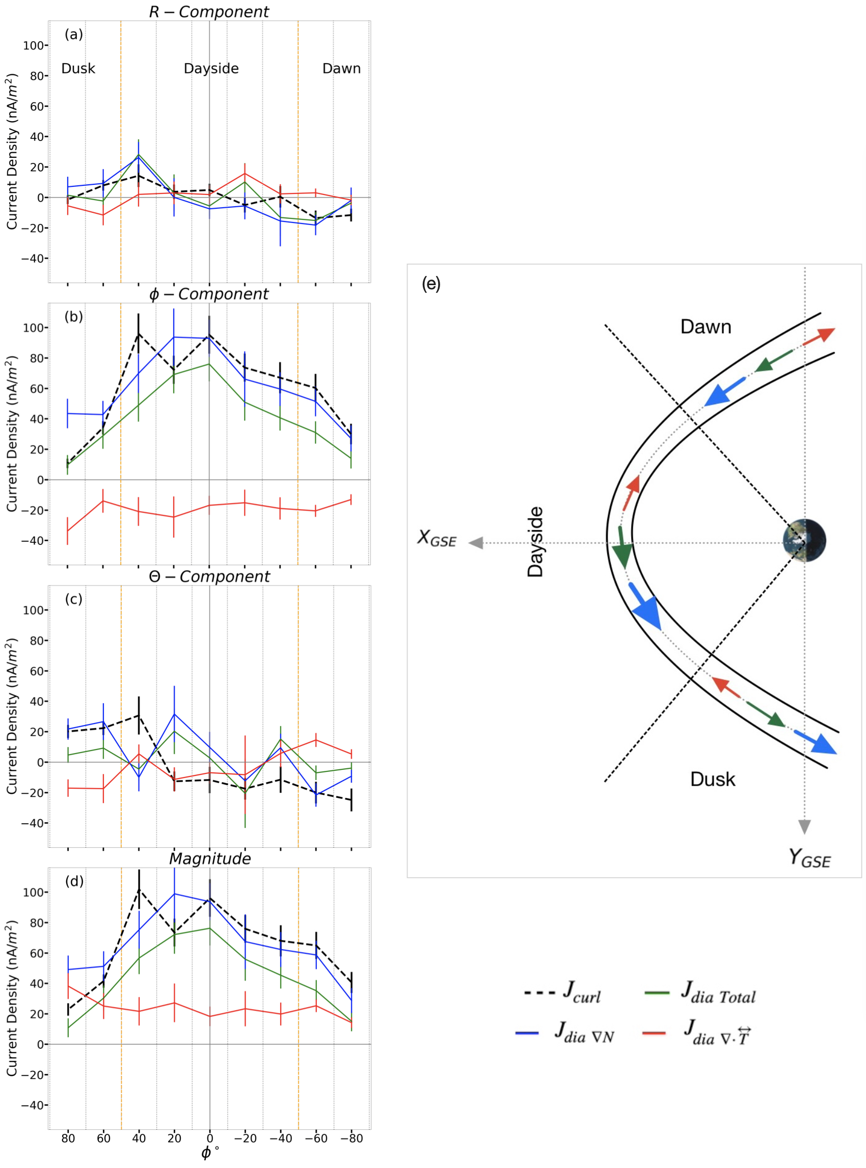
Figure 3: a) through d) depict current density accumulations for $\textbf{J}_{curl}$, $\textbf{J}_{dia\ Total}$, $\textbf{J}_{dia\ \nabla N}$, and $\textbf{J}_{dia\ \nabla\cdot\overleftrightarrow{T}}$ across the dayside and flank magnetopause sectors, represented by the orange dashed lines. The grey dashed lines represent the edges of the $20^{\circ}$ accumulation bins, centered at $80^{\circ}$, $60^{\circ}$, $40^{\circ}$, etc. Moving from top to bottom: a). represents the R-component of the current in our local spherical coordinate system (described in Figure 2). b). $\phi$ - component, c). $\theta$ - component, d). magnitude of the current components. e) diagram of the contributions and directions of $\textbf{J}_{dia\ Total}$, $\textbf{J}_{dia\ \nabla N}$, and $\textbf{J}_{dia\ \nabla\cdot\overleftrightarrow{T}}$ across the dusk, dayside, and dawn magnetopause. Note the size of the arrows in each sector indicates the relative magnitude of their current densities and the direction indicates the current component’s flow around the magnetopause.

2.5 Current Measurement Results

We then used our data to create a table of results over the dusk, dayside, and dawn magnetopause including the mean, median, and standard errors for our 561 magnetopause crossings as seen in Table 1.

From this table, $\textbf{J}_{curl}$ is strongest on the dayside, with a dusk-dawn asymmetry as the dawn curlometer current is stronger than the dusk. Both $\textbf{J}_{dia\ Total}$ and $\textbf{J}_{dia\ \nabla N}$ show similar distributions with the dayside again being the strongest sector, but the dusk and dawn results are now in agreement within their standard errors. The $\textbf{J}_{dia\ \nabla\cdot\overleftrightarrow{T}}$ component shows a dusk-dawn asymmetry with a significantly stronger dusk current density than the dawn. The total electron diamagnetic current, $\textbf{J}_{e\ dia\ Total}$, is the weakest current component studied and shows a dusk-dawn asymmetry with the dusk being significantly weaker than both the dusk and the dayside.

Comparing these results with past studies, our magnetopause thickness are, in general, higher than those found by Haaland2020; however, this is to be expected as we are considering a specific subset of database events as described in the previous sections. For similar reasons, the current densities found by Haaland2020 show differences, with our dawn current densities matching closely, but the dusk and dayside values showing deviations.

Table 1: Magnetopause parameters, magnitudes, and $\phi$ components of current densities across Dusk: ($+50^{\circ}$ to $+90^{\circ}$), Dawn: ($-50^{\circ}$ to $-90^{\circ}$), and Dayside: ( $>$ $-50^{\circ}$ and $<$ $+50^{\circ}$) crossings with the following format: mean (median) $\pm$ standard error of the values measured over each event’s magnetopause crossing. Note, $V_{n}$ values are unsigned averages and medians of the normal magnetopause velocity.

Parameter	Dusk	Dayside	Dawn
Number of Crossings	215	225	121
Thickness (km)	1961 (1429) $\pm$ 132	2032 (1379) $\pm$ 135	1950 (1393) $\pm$ 180
Thickness ($d_{i}$)	21.4 (14.3) $\pm$ 1.5	26.7 (16.4) $\pm$ 1.8	28.0 (15.9) $\pm$ 3.0
Thickness ($R_{gi}$)	35.6 (18.7) $\pm$ 4.3	85.9 (33.2) $\pm$ 12	33.2 (17.9) $\pm$ 4.0
$V_{n}$ (km/s)	131.5 (109.8) $\pm$ 7.0	99.8 (71.1) $\pm$ 7.5	94.3 (86.0) $\pm$ 6.3
Duration (s)	16.0 (11.2) $\pm$ 0.8	25.0 (18.7) $\pm$ 1.3	20.6 (14.7) $\pm$ 1.3
$|\textbf{J}_{curl}|$ $(nA/m^{2})$	30.0 (17.6) $\pm$ 3.2	83.2 (67.7) $\pm$ 5.6	52.1 (35.0) $\pm$ 6.3
$|\textbf{J}_{i\ dia\ Total}|$ $(nA/m^{2})$	19.4 (8.4) $\pm$ 5.8	59.0 (47.5) $\pm$ 6.9	25.1 (17.5) $\pm$ 5.0
$|\textbf{J}_{dia\ \nabla N_{i}}|$ $(nA/m^{2})$	50.0 (28.3) $\pm$ 8.5	78.2 (64.7) $\pm$ 7.2	43.6 (32.7) $\pm$ 6.6
$|\textbf{J}_{dia\ \nabla\cdot\overleftrightarrow{T}_{i}}|$ $(nA/m^{2})$	31.5 (16.6) $\pm$ 7.0	20.0 (13.5) $\pm$ 5.8	19.6 (10.8) $\pm$ 2.9
$\textbf{J}_{curl}\ ({\phi})$ $(nA/m^{2})$	21.1 (10.9) $\pm$ 2.7	83.0 (67.4) $\pm$ 5.3	45.3 (30.3) $\pm$ 5.9
$\textbf{J}_{i\ dia\ Total}\ ({\phi})$ $(nA/m^{2})$	18.2 (8.3) $\pm$ 5.2	58.7 (47.3) $\pm$ 5.2	22.6 (16.6) $\pm$ 5.0
$\textbf{J}_{dia\ \nabla N_{i}}\ ({\phi})$ $(nA/m^{2})$	43.2 (26.1) $\pm$ 6.7	78.0 (64.7) $\pm$ 6.7	39.4 (30.4) $\pm$ 6.6
$\textbf{J}_{dia\ \nabla\cdot\overleftrightarrow{T}_{i}}\ ({\phi})$ $(nA/m^{2})$	-25.0 (-16.1) $\pm$ 6.2	-19.3 (-13.3) $\pm$ 4.1	-16.8 (-10.7) $\pm$ 2.7
$|\textbf{J}_{e\ dia\ Total}|$ $(nA/m^{2})$	1.7 (0.5) $\pm$ 0.7	5.9 (4.4) $\pm$ 1.0	5.4 (3.6) $\pm$ 0.7

3 Temperature Gradient’s Impact on the Magnetopause Current System

Using our results from Figure 3 and Table 1, we can posit three primary ways the ion temperature gradient impacts the magnetopause current density and, in doing so, create a 2D diagram to summarize our findings as shown in Figure 3e.

1. The divergence of the ion temperature tensor generates up to one third of the total ion diamagnetic current density in the $\phi$ direction.

   Specifically, in the $\phi$ direction, the ratio of the temperature-driven component to the density-driven component’s contribution to the total ion diamagnetic current gives the following break down with $\textbf{J}_{dia\ \nabla\cdot\overleftrightarrow{T}}$ making up $37\%$ of the diamagnetic current density on the dusk, $20\%$ on the dayside, and $30\%$ on the dawn.

2. $\textbf{J}_{dia\ \nabla\cdot\overleftrightarrow{T}}$ goes in the opposite direction of the classical Chapman-Ferraro Current.

   $\textbf{J}_{dia\ \nabla\cdot\overleftrightarrow{T}}$ is clearly in the $-\phi$ direction across the magnetopause when considering Figure 3b and Table 1. This results in $\textbf{J}_{dia\ \nabla\cdot\overleftrightarrow{T}}$ lowering the contribution of $\textbf{J}_{dia\ \nabla N}$, making the $\textbf{J}_{dia\ Total}$ less than $\textbf{J}_{curl}$ on average as seen in Table 1.

3. $\textbf{J}_{dia\ \nabla\cdot\overleftrightarrow{T}}$’s contribution to the magnetopause current density becomes more important toward the flank magnetopause.

   $\textbf{J}_{dia\ Total}$ and $\textbf{J}_{dia\ \nabla N}$ are strongest on the dayside and grow steadily weaker on the dusk and the dawn flanks, with both flanks showing similar results for the current densities. This is in contrast to $\textbf{J}_{dia\ \nabla\cdot\overleftrightarrow{T}}$ which increases in strength, particularly on the dusk flank, resulting in the total diamagnetic current being decreased even further by $\textbf{J}_{dia\ \nabla\cdot\overleftrightarrow{T}}$’s impact on the flank mangetopause.

From Table 1 and Figure 3 we may also notice the difference between the curlometer and the total diamagnetic current densities across the magnetopause. This difference is generally expected as the curlometer current represents the total current density as measured by MMS across the magnetopause current layer, which includes contributions from both ion and electron currents and their perpendicular and parallel components. The total ion diamagnetic current is thus one component of the curlometer current. This being said, the total diamagnetic current density still represents the main contributor to the curlometer current, accounting for almost 70% of the current density on the dayside.

4 Discussion

4.1 Gradient Formation

These observations are generally consistent with previously literature regarding ion populations in the magnetosphere. From Chappell2008, the warm plasma cloak is defined as a population of 10 eV to 3 keV ions energized in the polar cap and magnetotail, which circulates in a dawn-to-dusk circulation pattern throughout the inner magnetosphere out to the magnetopause. As Chappell2008 notes, the warm plasma cloak ions can occupy the same space as the much warmer and more energetic ring current ions, which circulate in the opposite direction across the magnetosphere, from dusk-to-dawn. Thus it is possible, on a simplified level of magnetospheric circulation, that the colder warm plasma cloak ions provide generating pressure for the density gradient component across the magnetopause in its dawn-to-dusk, CF current like direction, while the warmer ring current ions provide generating pressure for the temperature gradient component in its dusk-to-dawn direction. The density component’s dayside-flank asymmetry could also be explained by additional density gradients generated by the plasmasphere drainage plume [Borovsky  Denton (2008)], which exhausts through the dayside magnetopause during storm conditions, enhancing the dayside with more cold ions, thus leading to an enhanced dayside $\textbf{J}_{dia\ \nabla N}$ while leaving the dusk and dawn components reliant solely on the warm plasma cloak ion population. The presence of magnetosphere particle populations in the mangetopause and their effects on the magnetopause current sheet, specifically regarding magnetic reconnection, is explored in the following studies: e.g. Borovsky2008, Fuselier2017, and Walsh2013. Additional study regarding the effects of the warm plasma cloak and plasmasphere particle populations on the diamagnetic current and its component generation is needed however.

4.2 Large Scale Current System Closure

From Figure 3 and Table 1, we can see the total diamagnetic current density is lower on the flanks, helped by an increasingly prominent temperature component. This indicates current closure with the larger 3D current system where the magnetopause current steadily curves toward the parallel as it goes around the flanks. As the total current through the magnetopause current system must remain constant, as charge is conserved, the current density of the total current’s components must then fluctuate appropriately along the dayside and flanks to “transfer” the current density from the perpendicular dominated dayside to the increasingly parallel dominated flanks. This indicates that the total diamagnetic (perpendicular) current decreases in order for more of the total current density to be diverted toward parallel currents such as the field aligned currents. Additionally, the magnetopause is generally thinner on the dayside and thicker on the flanks while the magnetopause current must remain the same as it flows through the magnetopause (e.g. Haaland2019,Haaland2020). Thus the total perpendicular current density must change to compensate for either a thinner or thicker magnetopause. From Figure 3, we can see this is, indeed, the case as the total diamagnetic current density decreases on the flanks and is strongest toward the dayside.

4.3 Ion vs. Electron Diamagnetic Current Densities

Even though the electron diamagnetic current was found to be significant on electron scale current sheets by Shuster2019,Shuster2021, we found the electron current density to be less significant over our ion scale magnetopause current sheets. Specifically the electron diamagnetic current density is $7\%$ of the ion diamagnetic current density in the $\phi$ direction on the dusk, $10\%$ on the dayside, and $20\%$ on the dawn. This presents an interesting asymmetry for the electron current as it is noticeably weaker on average on the dusk than it is on the dawn; however, in both cases, the electron diamagnetic current is also weaker than the contribution made by the ion current. The weaker electron current density may be explained based on the fact that we are averaging over many electron scale current sheets when considering our ion scale magnetopause crossing, thus lowering the resulting current density.

5 Conclusions

In this paper, we have quantified the diamagnetic current’s composite nature. Based on our systematic analysis of four years of MMS magnetopause crossings, the diamagnetic current is composed of two competing components: one generated by density gradients and one by temperature gradients.

We have found that the temperature generated component acts against the density component, weakening the total diamagnetic current’s net strength, particularly on the flanks where the temperature component’s contribution can reach up to 37% of the diamagnetic current density along the magnetopause. We also found that ions contribute the majority of the current density to the diamagnetic current, with electrons accounting for only 7% to 20% of the ion’s contribution.

Taking these findings into account, we can posit that enhancements of the temperature gradient along the magnetopause boundary may lead to a corresponding weakening of both the diamagnetic current and, by extension, the total current in the magnetopause. This implied weakening of the magnetopause current by the temperature gradient leads to a more complicated picture of the interaction between the solar wind and Earth’s magnetosphere, especially on small scales where situations can arise where the two components of the diamagnetic current become equal yet opposite, leading to the net cancellation of the diamagnetic current in that region. Studying the small-scale consequences of this interaction is the basis of our future work.

Open Research

The MMS data used in this study is publicly available at https://lasp.colorado.edu/mms/sdc/public/datasets/ from the FPI, FIELDS, and HPCA datasets. The averaged MMS data over the 561 MP crossings used for this study are available through a Harvard Dataverse public database: https://doi.org/10.7910/DVN/SRBJCR.

References

- Borovsky \BBA Denton (\APACyear2008) \APACinsertmetastarBorovsky2008{APACrefauthors}Borovsky, J\BPBIE.\BCBT \BBA Denton, M\BPBIH. \APACrefYearMonthDay2008. \BBOQ\APACrefatitleA statistical look at plasmaspheric drainage plumes A statistical look at plasmaspheric drainage plumes.\BBCQ \APACjournalVolNumPagesJournal of Geophysical Research: Space Physics113A9. {APACrefDOI} 10.1029/2007JA012994 \PrintBackRefs\CurrentBib
- Burch \BOthers. (\APACyear2015) \APACinsertmetastarMMS_paper{APACrefauthors}Burch, J\BPBIL., Moore, T\BPBIE., Torbet, R\BPBIB.\BCBL \BBA Giles, B\BPBIL. \APACrefYearMonthDay2015. \BBOQ\APACrefatitleMagnetospheric Multiscale Overview and Science Objectives Magnetospheric multiscale overview and science objectives.\BBCQ \APACjournalVolNumPagesSpace Science Review1995-21. {APACrefDOI} 10.1007/s11214-015-0164-9 \PrintBackRefs\CurrentBib
- Cahill \BBA Amazeen (\APACyear1963) \APACinsertmetastarCahill1963{APACrefauthors}Cahill, L\BPBIJ.\BCBT \BBA Amazeen, P\BPBIG. \APACrefYearMonthDay1963. \BBOQ\APACrefatitleThe boundary of the geomagnetic field The boundary of the geomagnetic field.\BBCQ \APACjournalVolNumPagesJournal of Geophysical Research6871835-1843. {APACrefDOI} 10.1029/JZ068i007p01835 \PrintBackRefs\CurrentBib
- Chapman \BBA Ferraro (\APACyear1931) \APACinsertmetastarCF1931{APACrefauthors}Chapman, S.\BCBT \BBA Ferraro, V\BPBIC\BPBIA. \APACrefYearMonthDay1931. \BBOQ\APACrefatitleA new theory of magnetic storms A new theory of magnetic storms.\BBCQ \APACjournalVolNumPagesTerrestrial Magnetism and Atmospheric Electricity3677-97. \PrintBackRefs\CurrentBib
- Chappell \BOthers. (\APACyear2008) \APACinsertmetastarChappell2008{APACrefauthors}Chappell, C\BPBIR., Huddleston, M\BPBIM., Moore, T\BPBIE., Giles, B\BPBIL.\BCBL \BBA Delcourt, D\BPBIC. \APACrefYearMonthDay2008. \BBOQ\APACrefatitleObservations of the warm plasma cloak and an explanation of its formation in the magnetosphere Observations of the warm plasma cloak and an explanation of its formation in the magnetosphere.\BBCQ \APACjournalVolNumPagesJournal of Geophysical Research113A09206. {APACrefDOI} 10.1029/2007JA012945 \PrintBackRefs\CurrentBib
- Dong \BOthers. (\APACyear2018) \APACinsertmetastarDong2018{APACrefauthors}Dong, X\BPBIC., Dunlop, M\BPBIW., Wang, T\BPBIY., Cao, J\BPBIB., Trattner, K\BPBIJ., Bamford, R.\BDBLTorbert, R\BPBIB. \APACrefYearMonthDay2018. \BBOQ\APACrefatitleCarriers and Sources of Magnetopause Current: MMS Case Study Carriers and sources of magnetopause current: Mms case study.\BBCQ \APACjournalVolNumPagesJournal of Geophysical Research: Space Physics1235464–5475. {APACrefDOI} https:// doi.org/10.1029/2018JA025292 \PrintBackRefs\CurrentBib
- Dunlop \BOthers. (\APACyear1988) \APACinsertmetastarDunlop1988{APACrefauthors}Dunlop, M\BPBIW., Southwood, D\BPBIJ., Glassmeier, K\BHBIH.\BCBL \BBA Neubauer, F\BPBIM. \APACrefYearMonthDay1988. \BBOQ\APACrefatitleAnalysis of multipoint magnetometer data Analysis of multipoint magnetometer data.\BBCQ \APACjournalVolNumPagesAdvanced Space Research8273-277. \PrintBackRefs\CurrentBib
- Fuselier \BOthers. (\APACyear2019) \APACinsertmetastarFuselier2019{APACrefauthors}Fuselier, S\BPBIA., Mukherjee, J., M. H. Denton, S\BPBIM\BPBIP., Trattner, K\BPBIJ., Toledo-Redondo, S., André, M.\BDBLBurch, J\BPBIL. \APACrefYearMonthDay2019. \BBOQ\APACrefatitleHigh-density in Earth’s outer magnetosphere and its effect on dayside magnetopause magnetic reconnection High-density in earth’s outer magnetosphere and its effect on dayside magnetopause magnetic reconnection.\BBCQ \APACjournalVolNumPagesJournal of Geophysical Research: Space Physics1241210257–10269. {APACrefDOI} https://doi.org/10.1029/2019JA027396 \PrintBackRefs\CurrentBib
- Fuselier \BOthers. (\APACyear2017) \APACinsertmetastarFuselier2017{APACrefauthors}Fuselier, S\BPBIA., Vines, S\BPBIK., Burch, J\BPBIL., Petrinec, S\BPBIM., Trattner, K\BPBIJ., Cassak, P.\BDBLWebster, J\BPBIM. \APACrefYearMonthDay2017. \BBOQ\APACrefatitleLarge-scale characteristics of reconnection diffusion regions and associated magnetopause crossings observed by MMS Large-scale characteristics of reconnection diffusion regions and associated magnetopause crossings observed by mms.\BBCQ \APACjournalVolNumPagesJournal of Geophysical Research: Space Weather1225466-5486. {APACrefDOI} doi:10.1002/2017JA024024. \PrintBackRefs\CurrentBib
- Ganushkina \BOthers. (\APACyear2018) \APACinsertmetastarGanushkina2017{APACrefauthors}Ganushkina, N\BPBIY., Liemohn, M\BPBIW.\BCBL \BBA Dubyagin, S. \APACrefYearMonthDay2018. \BBOQ\APACrefatitleCurrent Systems in the Earth’s Magnetosphere Current systems in the earth’s magnetosphere.\BBCQ \APACjournalVolNumPagesReviews of Geophysics56309–332. {APACrefDOI} https://doi.org/10.1002/2017RG000590 \PrintBackRefs\CurrentBib
- Haaland \BOthers. (\APACyear2020) \APACinsertmetastarHaaland2020{APACrefauthors}Haaland, S., Paschmann, G., Øieroset, M., Phan, T., Hasegawa, H., Fuselier, S\BPBIA.\BDBLBurch, J. \APACrefYearMonthDay2020. \BBOQ\APACrefatitleCharacteristics of the Flank Magnetopause: MMS Results Characteristics of the flank magnetopause: Mms results.\BBCQ \APACjournalVolNumPagesJournal of Geophysical Research: Space Physics125. {APACrefDOI} https://doi.org/ 10.1029/2019JA027623 \PrintBackRefs\CurrentBib
- Haaland \BOthers. (\APACyear2014) \APACinsertmetastarHaaland2014{APACrefauthors}Haaland, S., Reistad, J., Tenfjord, P., Gjerloev, J., Maes, L., DeKeyser, J.\BDBLDorville, N. \APACrefYearMonthDay2014. \BBOQ\APACrefatitleCharacteristics of the flank magnetopause: Cluster observations Characteristics of the flank magnetopause: Cluster observations.\BBCQ \APACjournalVolNumPagesJournal of Geophysical Research: Space Physics1199019–9037. {APACrefDOI} doi:10.1002/2014JA020539 \PrintBackRefs\CurrentBib
- Haaland \BOthers. (\APACyear2019) \APACinsertmetastarHaaland2019{APACrefauthors}Haaland, S., Runov, A., Artemyev, A.\BCBL \BBA Angelopoulos, V. \APACrefYearMonthDay2019. \BBOQ\APACrefatitleCharacteristics of the Flank Magnetopause: THEMIS Observations Characteristics of the flank magnetopause: Themis observations.\BBCQ \APACjournalVolNumPagesJournal of Geophysical Research: Space Physics1243421–3435. {APACrefDOI} https://doi. org/10.1029/2019JA026459 \PrintBackRefs\CurrentBib
- Hasegawa (\APACyear2012) \APACinsertmetastarHasegawa2012{APACrefauthors}Hasegawa, H. \APACrefYearMonthDay2012. \BBOQ\APACrefatitleStructure and Dynamics of the Magnetopause and Its Boundary Layers Structure and dynamics of the magnetopause and its boundary layers.\BBCQ \APACjournalVolNumPagesMonogr. Environ. Earth Planets1271-119. {APACrefDOI} 10.5047/meep.2012.00102.0071 \PrintBackRefs\CurrentBib
- Khrabrov \BBA Sonnerup (\APACyear1998a) \APACinsertmetastarKhrabrov1998a{APACrefauthors}Khrabrov, A\BPBIV.\BCBT \BBA Sonnerup, B\BPBIU\BPBIO. \APACrefYearMonthDay1998a. \BBOQ\APACrefatitledeHoffmann-Teller analysis dehoffmann-teller analysis.\BBCQ \BIn \APACrefbtitleAnalysis methods for multi-spacecraft data Analysis methods for multi-spacecraft data (\BPG 221). \APACaddressPublisherNoordwijkESA Publication Division. \PrintBackRefs\CurrentBib
- Le \BBA Russell (\APACyear1994) \APACinsertmetastarLe1994{APACrefauthors}Le, G.\BCBT \BBA Russell, C\BPBIT. \APACrefYearMonthDay1994. \BBOQ\APACrefatitleThe thickness and structure of high beta magnetopause current layer The thickness and structure of high beta magnetopause current layer.\BBCQ \APACjournalVolNumPagesGeophysical Research Letters21232451-2454. {APACrefDOI} https://doi.org/10.1029/94GL02292 \PrintBackRefs\CurrentBib
- Paschmann \BOthers. (\APACyear2018) \APACinsertmetastarPaschmann2018{APACrefauthors}Paschmann, G., Haaland, S\BPBIE., Phan, T., Sonnerup, B., Burch, J., Torbert, R.\BDBLFuselier, S. \APACrefYearMonthDay2018. \BBOQ\APACrefatitleLarge-Scale Survey of the Structure of the Dayside Magnetopause by MMS Large-scale survey of the structure of the dayside magnetopause by mms.\BBCQ \APACjournalVolNumPagesJournal of Geophysical Research: Space Physics1232018–2033. {APACrefDOI} https://doi.org/10.1002/2017JA025121 \PrintBackRefs\CurrentBib
- Paschmann \BOthers. (\APACyear2020) \APACinsertmetastarPaschmann2020{APACrefauthors}Paschmann, G., Sonnerup, B., Haaland, S\BPBIE., Phan, T.\BCBL \BBA Denton, R\BPBIE. \APACrefYearMonthDay2020. \BBOQ\APACrefatitleComparison of Quality Measures for Walén Relation Comparison of quality measures for walén relation.\BBCQ \APACjournalVolNumPagesJournal of Geophysical Research: Space Physics125e2020JA028044. {APACrefDOI} https://doi.org/ 10.1029/2020JA028044 \PrintBackRefs\CurrentBib
- Phan \BOthers. (\APACyear1996) \APACinsertmetastarPhanLarson1996{APACrefauthors}Phan, T\BPBID., Larson, D\BPBIE., Lin, R\BPBIP., McFadden, J\BPBIP., Anderson, K\BPBIA., Carlson, C\BPBIW.\BDBLSzabo, A. \APACrefYearMonthDay1996. \BBOQ\APACrefatitleThe subsolar magnetosheath and magnetopause for high solar wind ram pressure: WIND observations The subsolar magnetosheath and magnetopause for high solar wind ram pressure: Wind observations.\BBCQ \APACjournalVolNumPagesGeophysical Research Letters23101279-1282. {APACrefDOI} https://doi.org/10.1029/96GL00845 \PrintBackRefs\CurrentBib
- Phan \BBA Paschmann (\APACyear1996) \APACinsertmetastarPhanPaschmann1996{APACrefauthors}Phan, T\BPBID.\BCBT \BBA Paschmann, G. \APACrefYearMonthDay1996. \BBOQ\APACrefatitleLow-latitude dayside magnetopause and boundary layer for high magnetic shear: 1. Structure and motion Low-latitude dayside magnetopause and boundary layer for high magnetic shear: 1. structure and motion.\BBCQ \APACjournalVolNumPagesJournal of Geophysical Research: Space Physics101A47801-7815. {APACrefDOI} https://doi.org/10.1029/95JA03752 \PrintBackRefs\CurrentBib
- Pollock \BOthers. (\APACyear2016) \APACinsertmetastarFPI{APACrefauthors}Pollock, C., Moore, T., Jacques, A., Burch, J., Gliese, U., Saito, Y.\BDBLet al \APACrefYearMonthDay2016. \BBOQ\APACrefatitleFast Plasma Investigation for Magnetospheric Multiscale Fast plasma investigation for magnetospheric multiscale.\BBCQ \APACjournalVolNumPagesSpace Science Reviews199331-406. {APACrefDOI} https://doi.org/10.1007/s11214-016-0245-4 \PrintBackRefs\CurrentBib
- Russell \BOthers. (\APACyear2016) \APACinsertmetastarFGM{APACrefauthors}Russell, C\BPBIT., Anderson, B\BPBIJ., Baumjohann, W., Bromund, K\BPBIR., Dearborn, D., Fischer, D.\BDBLRichter, I. \APACrefYearMonthDay2016. \BBOQ\APACrefatitleThe Magnetospheric Multiscale Magnetometers The magnetospheric multiscale magnetometers.\BBCQ \APACjournalVolNumPagesSpace Science Reviews199189-256. {APACrefDOI} https://doi.org/10.1007/s11214-014-0057-3 \PrintBackRefs\CurrentBib
- Shuster \BOthers. (\APACyear2019) \APACinsertmetastarShuster2019{APACrefauthors}Shuster, J\BPBIR., Gershman, D\BPBIJ., Chen, L\BHBIJ., Wang, S., Bessho, N., Dorelli, J\BPBIC.\BDBLViñas, A\BPBIF. \APACrefYearMonthDay2019. \BBOQ\APACrefatitleMMS Measurements of the Vlasov Equation: Probing the Electron Pressure Divergence Within Thin Current Sheets Mms measurements of the vlasov equation: Probing the electron pressure divergence within thin current sheets.\BBCQ \APACjournalVolNumPagesGeophysical Research Letters46. {APACrefDOI} https://doi.org/10.1029/2019GL083549 \PrintBackRefs\CurrentBib
- Shuster \BOthers. (\APACyear2021) \APACinsertmetastarShuster2021{APACrefauthors}Shuster, J\BPBIR., Gershman, D\BPBIJ., Dorelli, J\BPBIC., Giles, B\BPBIL., Wang, S., Bessho, N.\BDBLTorbert, R\BPBIB. \APACrefYearMonthDay2021. \BBOQ\APACrefatitleStructures in the terms of the Vlasov equation observed at Earth’s magnetopause Structures in the terms of the vlasov equation observed at earth’s magnetopause.\BBCQ \APACjournalVolNumPagesNature Physics. {APACrefDOI} https://doi.org/10.1038/s41567-021-01280-6 \PrintBackRefs\CurrentBib
- Sonnerup \BBA Scheible (\APACyear1998) \APACinsertmetastarSonnerup1998{APACrefauthors}Sonnerup, B\BPBIU\BPBIO.\BCBT \BBA Scheible, M. \APACrefYearMonthDay1998. \BBOQ\APACrefatitleMinimum and maximum variance analysis Minimum and maximum variance analysis.\BBCQ \BIn \APACrefbtitleAnalysis methods for multi-spacecraft data Analysis methods for multi-spacecraft data (\BPG 1850). \APACaddressPublisherNoordwijkESA Publication Division. \PrintBackRefs\CurrentBib
- Walsh \BOthers. (\APACyear2013) \APACinsertmetastarWalsh2013{APACrefauthors}Walsh, B\BPBIM., Sibeck, D\BPBIG., Nishimura, Y.\BCBL \BBA Angelopoulos, V. \APACrefYearMonthDay2013. \BBOQ\APACrefatitleStatistical analysis of the plasmaspheric plume at the magnetopause Statistical analysis of the plasmaspheric plume at the magnetopause.\BBCQ \APACjournalVolNumPagesJournal of Geophysical Research: Space Physics11884844-4851. {APACrefDOI} https://doi.org/10.1002/jgra.50458 \PrintBackRefs\CurrentBib
- Young \BOthers. (\APACyear2016) \APACinsertmetastarHPCA{APACrefauthors}Young, D\BPBIT., Burch, J\BPBIL., Gomez, R\BPBIG., Santos, A\BPBID\BPBIL., Miller, G\BPBIP., IV, P\BPBIW.\BDBLWebster, J\BPBIM. \APACrefYearMonthDay2016. \BBOQ\APACrefatitleHot Plasma Composition Analyzer for the Magnetospheric Multiscale Mission Hot plasma composition analyzer for the magnetospheric multiscale mission.\BBCQ \APACjournalVolNumPagesSpace Science Reviews199407-470. {APACrefDOI} https://doi.org/10.1007/s11214-014-0119-6 \PrintBackRefs\CurrentBib