Online Discrepancy with Recourse for Vectors and Graphs

Abstract

The vector-balancing problem is a fundamental problem in discrepancy theory: given $T$ vectors in $[-1,1]^{n}$, find a signing $\sigma(a)\in\{\pm 1\}$ of each vector $a$ to minimize the discrepancy $\|\sum_{a}\sigma(a)\cdot a\|_{\infty}$. This problem has been extensively studied in the static/offline setting. In this paper we initiate its study in the fully-dynamic setting with recourse: the algorithm sees a stream of $T$ insertions and deletions of vectors, and at each time must maintain a low-discrepancy signing, while also minimizing the amortized recourse (the number of times any vector changes its sign) per update.

For general vectors, we show algorithms which almost match Spencer’s $O(\sqrt{n})$ offline discrepancy bound, with ${O}(n\operatorname{poly}\!\log T)$ amortized recourse per update. The crucial idea behind our algorithm is to compute a basic feasible solution to the linear relaxation in a distributed and recursive manner, which helps find a low-discrepancy signing. We bound the recourse using the distributed computation of the basic solution, and argue that only a small part of the instance needs to be re-computed at each update.

Since vector balancing has also been greatly studied for sparse vectors, we then give algorithms for low-discrepancy edge orientation, where we dynamically maintain signings for $2$-sparse vectors in an $n$-dimensional space. Alternatively, this can be seen as orienting a dynamic set of edges of an $n$-vertex graph to minimize the discrepancy, i.e., the absolute difference between in- and out-degrees at any vertex. We present a deterministic algorithm with $O(\operatorname{poly}\!\log n)$ discrepancy and $O(\operatorname{poly}\!\log n)$ amortized recourse. The core ideas are to dynamically maintain an expander-decomposition with low recourse (using a very simple approach), and then to show that, as the expanders change over time, a natural local-search algorithm converges quickly (i.e., with low recourse) to a low-discrepancy solution. We also give strong lower bounds (with some matching upper bounds) for local-search discrepancy minimization algorithms for vector balancing and edge orientation.

1 Introduction

In the Online Vector Balancing problem introduced by Spencer [Spe77], vectors $a_{1},a_{2},\ldots,a_{T}\in[-1,1]^{n}$ arrive online, and the algorithm irrevocably assigns a sign $\sigma(a_{t})$ immediately upon seeing $a_{t}$, with the goal of minimizing the discrepancy of the signed sum, i.e., $\|\sum_{t}\sigma(a_{t})\cdot a_{t}\|_{\infty}$. Following a sequence of works [BS20, BJSS20, BJM⁺21], the state-of-the-art bounds for this problem is an elegant randomized algorithm that maintains a discrepancy of $O(\sqrt{n}\log(nT))$ [ALS21]. Their result assumes an oblivious adversary, so that the choice of arriving vectors does not depend on the internal state of the algorithm. Indeed, if we allow adaptive adversaries then every online algorithm incurs $\Omega(\sqrt{T})$ discrepancy [Spe77]. We think of $T\gg n$, so $\Omega(\sqrt{T})$ is much larger than $O(\sqrt{n}\log(nT))$.

We initiate the study of Fully-Dynamic Vector Balancing, where vectors can both arrive or depart at each time step, and the algorithm must always maintain a low-discrepancy signing of the vectors present in the system at all times. Since it is easy to construct examples where no algorithm can guarantee non-trivial discrepancy bounds if it is forced to commit to the sign of a vector upon arrival, we study the problem where the algorithm can re-sign the vectors from time to time. Indeed, many real-world applications that motivate such discrepancy-based methods (such as in fair allocations, sparsification routines, etc.) have a fully-dynamic flavor to them, with the corresponding inputs being dynamic in nature due to both insertions and deletions.

Problem (Fully-Dynamic Vector Balancing). We start with an empty collection of active vectors $A(0)$. At each time/update $t\in[T]$, an adaptive adversary either inserts a new vector $a_{t}\in[-1,1]^{n}$, i.e., $A(t)=A(t-1)\cup\{a_{t}\}$, or removes an existing vector $a\in A(t-1)$, i.e., $A(t)=A(t-1)\setminus\{a\}$. The goal is to maintain signings $\sigma_{t}:A(t)\rightarrow\{\pm 1\}$ to minimize the norm $\|\sum_{a\in A(t)}\sigma_{t}(a)\cdot a\|_{\infty}$. The algorithm can reassign the sign of a vector $a$ (i.e., set $\sigma_{t}(a)\neq\sigma_{t-1}(a)$), and the total recourse is the sum total of the reassignments.

Two trivial solutions exist: (a) recomputing low-discrepancy signings on the active set of vectors after every update operation incurs optimal offline discrepancy guarantees with a recourse of $\Theta(T)$ per update, and (b) an independent and uniformly random signing of every new vector maintains at any time $t$ a signing of discrepancy $\Theta(\sqrt{T\log n})$ w.h.p., while performing no recourse whatsoever. Since $T\gg n$, this is much larger than the optimal offline discrepancy bounds of $O(\sqrt{n})$ for any collection of $T$ vectors in $[-1,1]^{n}$ [Spe85, Ban10, LM15]. We ask: can we get near-optimal discrepancy bounds with a small amount of recourse?

1.1 Our Results and Techniques

Fully-Dynamic Vector Balancing.

Our first main contribution is the design of an algorithm which maintains low-discrepancy signings for the fully-dynamic problem that nearly matches the offline discrepancy bounds while giving an amortized recourse that is only logarithmic in the sequence length $T$.

Theorem 1.1 (Fully-Dynamic: General Vector Balancing).

There is an efficient algorithm for Fully-Dynamic Vector Balancing with update vectors in $[-1,1]^{n}$ which maintains signings $\sigma_{t}(\cdot)$ with discrepancy $O(\sqrt{n})$ and an amortized recourse of $O(n\log T)$ per update, even against adaptive adversaries. For Komlos’ setting, i.e., if all the updates vectors have $\ell_{2}$ length at most $1$ (instead of $\ell_{\infty}$ length), the algorithm achieves discrepancy $O(\sqrt{\log(n)})$ with an amortized recourse of $O(n\log T)$ per update.

Since in this theorem we are competitive against adaptive adversaries, it illustrates the power of recourse: in the absence of recourse, we get $\Omega(\sqrt{T})$ lower bounds on the discrepancy even for arrival-only sequences of $2$-dimensional vectors. This is because the adversary can always make the next vector to be orthogonal to the current signed sum.

At a very high level, our algorithm divides the instance into many parts of size $O(n)$, obtains a good partial signing for each part (such that all but $n$ vectors are signed), and recurses on the residual instance. The algorithm imposes a tree-like hierarchy on these parts, so that it can easily adapt to inserts or deletes with bounded recourse by only re-running the computations on the part suffering the insertion/deletion, and on any internal node on the corresponding root-leaf path from that part to the root. If we are not careful, the discrepancy of the overall vector can be proportional to the number of parts, since we could accrue error in each part. However, we use linear algebraic ideas inspired by [BG81] to couple all the parts, thereby always ensuring that the sum of the partial signings across all nodes of the tree (except the root) is zero.

Fully-Dynamic Edge Orientation/Carpooling and Local Search.

Given the general result above, next we focus on the special case of orienting edges of a graph to minimize the maximum imbalance between the in- and out-degrees. Fagin and Williams [FW83] posed the carpooling problem, which corresponds to vector balancing with vectors of the form $(0,\ldots,0,1,0,\ldots,0,-1,0,\ldots)\in\mathbb{R}^{n}$, and the graph discrepancy objective is precisely the $\|\cdot\|_{\infty}$ of the signed sum of vectors. [FW83, AAN⁺98] use this problem to model fairness in scheduling, where edges represent shared commitments (such as carpooling), orientations give primary and secondary partners of the commitment (e.g., driver and co-driver), and hence the discrepancy measures fairness for individuals, in terms of how many commitments he/she is the primary partner for, relative to the total number of commitments he/she is a part of.

Somewhat surprisingly, [AAN⁺98] showed that any algorithm must suffer $\Omega(n)$ discrepancy on some worse-case adaptive sequence of edge arrivals. On the other hand, for an oblivious sequence of edge arrivals, it is easy to maintain orientations with $O(\sqrt{n\log n})$ discrepancy by simply orienting edges randomly (while always orienting repeated parallel edges $(u,v)$ oppositely). To mitigate such strong lower bounds, [AAN⁺98] and recently Gupta et al. [GKKS20] study a stochastic version of the problem where the arriving edges are sampled from a known distribution: they design algorithms to maintain $\operatorname{poly}\!\log(n,T)$-discrepancy. The recent algorithm of Alweiss et al. [ALS21] also extends to this special case giving $O(\log(nT))$ discrepancy bounds for any oblivious sequence of edge arrivals, not just stochastic ones. None of these prior algorithms extend to a fully-dynamic input consisting of both insertions and deletions. Moreover, Theorem 1.1 guarantees near-optimal discrepancy only with $O(n\log T)$ amortized recourse. In this paper, we give deterministic near-optimal discrepancy algorithms with near-optimal amortized recourse.

Theorem 1.2 (Fully-Dynamic Edge Orientation).

There is an efficient deterministic algorithm that maintains an orientation of $\operatorname{poly}\!\log n$ discrepancy while performing an amortized recourse of $\operatorname{poly}\!\log n$ per update.

Since this algorithm is deterministic, the guarantees also hold against adaptive adversaries: there are $\Omega(n)$ discrepancy bounds for no-recourse algorithms against such adversaries, even for the setting of only arrivals.

At a high level, our algorithm can be seen as a composition of two modules. Firstly, we consider a simple local-search procedure, which flips an edge from $u\rightarrow v$ to $v\rightarrow u$ if the current discrepancy of $v$ exceeds that of $u$ by more than $2$. Clearly, this reduces the discrepancy of the maximum of these two vertices. Our crucial observation is that this process always maintains low-discrepancy signings when the graph is an expander. We find this interesting, since we can show that there are bad local optima with $\operatorname{poly}(n)$ discrepancy for general graphs. Secondly, we show how to dynamically maintain a partitioning of the edge set of an arbitrary graph $G$ into a disjoint collection of expanders $G_{1},G_{2},\ldots,G_{\ell}$ with each vertex appearing in at most $\operatorname{poly}\!\log n$ many expanders, such that the amortized number of changes to $G_{1}$, $G_{2}$, $\ldots,G_{\ell}$, per update to $G$ is bounded. (This expander decomposition can be viewed as a “preconditioning” step.) We build on ideas recently developed for dynamic graph algorithms [SW19, BvdBG⁺20]: our challenge is to show that dynamic expander decomposition can be done along with local search on the individual expanders, and specifically to control the potential functions that guide our proofs.

Indeed, using the above two modules to obtain Theorem 1.2 requires new ideas. When an update (insertion or deletion) occurs to $G$, we first modify our expander decomposition, and re-run local search starting from the prior local optima in each expander. While this ensures good discrepancy bounds, it could lead to many local search moves. In order to bound the latter quantity, our idea is to use a potential function in each expander to bound the recourse, such that each step of local search always decreases the potential by at least a constant. This is somewhat delicate: a single update in $G$ can change any particular expander $G_{i}$ by a lot (even though the amortized recourse is bounded), and hence the single-step potential change can be huge. We show how to maintain some Lipschitzness properties for our potential function under inserts and deletes, which gives us the final bounds of $\operatorname{poly}\!\log n$ on both the discrepancy and the recourse.

Along the way, we also develop a better understanding of the strengths and limitations of local search as a technique for discrepancy minimization problems, both for graphs and for general vectors.

Theorem 1.3 (Informal: Discrepancy of Local Optima).

For edge orientation in expanders, any locally optimal solution for local search using the simple potential $\Phi=\sum_{v\in V}disc(v)^{2}$ has discrepancy $O(\log n)$. For arbitrary graphs, however, the discrepancy can be as bad as $\Omega(n^{1/3})$. For general vectors in $\{\pm 1\}^{n}$ (and in $[-1,1]^{n}$), the local search bound using the simple potential $\Phi=\sum_{i\in[n]}\big{(}\sum_{t}\sigma(a_{t})\cdot a_{t}(i)\big{)}^{2}$ deteriorates to $\Omega(2^{n})$ (and to $\Omega(\sqrt{T})$).

Signing $s$-Sparse Vectors for Online Arrivals. Finally, we consider the problem with $s$-sparse vectors, which interpolates between the graphical case of $s=2$ and the general case. In the offline setting, the classical linear-algebraic algorithm of Beck and Fiala [BF81] constructs a signing with disrepancy $2s-1$ (independent of $n$ and $T$). Subsequent works by Banaszczyk [Ban98] and Bansal, Dadush, and Garg [BDG16] develop techniques to get discrepancy $O(\sqrt{s\log n})$, and a long-standing question in discrepancy theory is to improve this bound to $O(\sqrt{s})$. Here we study the Online Vector Balancing problem only with arrivals. In this setting, the algorithm of [ALS21] maintains signings of discrepancy $O(\sqrt{s}\log(nT))$ without recourse, but against an oblivious adversary. In Section 6 we give a generic reduction that can maintain near-optimal discrepancy for Online Vector Balancing against adaptive adversaries, with small recourse.

Theorem 1.4 (Arrivals Only: Online Vector Balancing with Recourse).

There is an efficient algorithm for Online Vector Balancing with $s$-sparse vectors that achieves $O(\sqrt{s\log n}\log T)$ discrepancy and $O(\log T)$ amortized recourse per update against an adaptive adversary.

1.2 Further Related Work

Discrepancy theory is a rich and vibrant area of research [Cha01, Mat09]. While some initial works [Spe77, Bá79] focused on the online discrepancy problem, the majority of research dealt with the offline setting, where the $T$ vectors are given upfront. Near-optimal results are known for settings such as discrete set systems [Spe85, Ban10, LM15] (i.e., vectors in $\{0,1\}^{n}$), sparse set systems [BF81] ($s$-sparse binary vectors), and general vectors in the unit ball [Ban98, Bec81, Gia97, Rot14, BDGL19].

There has been a renewed interest in the online discrepancy setting, where many of the techniques developed for the offline setting no longer extend. Most of the results for online vector discrepancy deal with stochastic settings of the problem where the arriving vectors satisfy some distributional assumptions [AAN⁺98, BS20, BJM⁺21]. A recent breakthrough work [ALS21] gives a very elegant randomized algorithm with near-optimal discrepancy for general vectors arriving online. However, to the best of our knowledge, none of these ideas easily extend to the fully-dynamic setting where vectors can also depart—which is the focus of this paper. In fact, we do not know how to adapt existing ideas to establish non-trivial results for even the simple deletions-only setting: starting with $T$ vectors, a uniformly random subset of $\nicefrac{{T}}{{2}}$ of these vectors are deleted one-by-one. Can we always maintain a low-discrepancy signing of the remaining vectors with small recourse?

The study of dynamic algorithms also has a rich history, both in the recourse model, which measures the number of updates made the algorithm per update, and the update-time model, which measures the running time of the algorithm per update. Apart from graph problems, these models have been studied in a variety of settings such network design [IW91, GK14, GGK16, ŁOP⁺15], clustering [GKLX20, CAHP⁺19], matching [GKKV95, CDKL09, BLSZ14], and scheduling [PW93, Wes00, AGZ99, SSS09, SV10, EL14, GKS14], and set cover [BHI18, BCH17, BK19, AAG⁺19, BHN19, BHNW20, GKKP17].

A different version of edge-orientation, commonly known as graph balancing, involves minimizing just the maximum in-degree (see, e.g., [BF99, Kow07, KKPS14]): the techniques used for that version seem quite different from those needed here.

Paper Outline.

We present the results for Fully-Dynamic Vector Balancing and specifically Theorem 1.1 in §2. The results for graph balancing appear in §3. Other results for local-search algorithms appear in §4 and §5. We close with an insertion-only algorithm for sparse vectors, and conclusions and open problems in §6.

2 Fully-Dynamic Vector Balancing

In this section, we prove Theorem 1.1. Given a set of vectors $a_{1},a_{2},\ldots,a_{T}\in[-1,1]^{n}$, the Bárány-Grinberg algorithm signs them such that the discrepancy of the signed sum is at most $2n$. However, this signing is highly sensitive to insert or delete operations. We address this issue by recursively dividing the input sequence such that we lose only $O(n)$ discrepancy at each level of this recursion tree—we call this the distributed Bárány-Grinberg algorithm. We then show how it can easily handle insert and delete operations with low recourse.

The main idea underlying the Bárány-Grinberg algorithm [BG81] is the following linear algebraic lemma.

Lemma 2.1 (Rounding Lemma [BG81]).

Let $a_{1},a_{2},\ldots,a_{T}\in[-1,1]^{n}$ be the columns of matrix $A\in[-1,1]^{n\times T}$. For any initial fractional signing $x\in[-1,1]^{T}$, there exists a (near-integral) signing $y$ with all but $n$ variables being $\pm 1$ such that $Ay=Ax$.

The signing $y$ is obtained by moving to a basic feasible solution (BFS) of the following set of linear constraints $\{Ay=Ax,\;y\in[-1,1]^{T}\}$, where $x$ is treated as being fixed. Based on Lemma 2.1, Bárány and Grinberg [BG81] gave the following offline algorithm: starting with the all-zeros vector as the fractional signing (i.e., $x=\bf{0}$), let $y$ be the almost-integral vector satisfying $Ay=0$. Now randomly rounding the fractional variables (with bias given by the $y_{i}$ values) and using concentration bounds shows a discrepancy of $O(\sqrt{n\log n})$, or using sophisticated rounding schemes can give the tight $O(\sqrt{n})$ discrepancy [Spe85, Ban10, LM15].

2.1 An Equivalent, Recursive Viewpoint

A natural question is: can we extend the above Bárány-Grinberg algorithm to the dynamic case? Naively using the rounding lemma does not work, since the rounded solutions $y$ and $y^{\prime}$ for matrices $A$ and $A^{\prime}$ differing in one column could be very different. Our idea is to simulate the Bárány-Grinberg algorithm in a distributed and recursive manner. We divide the sequence $\{1,\ldots,T\}$ into sub-sequences of length $2n$ each, which gives us a set of $m:=T/2n$ sub-sequences (assume w.l.o.g., e.g., by padding, that $T/2n$ is a power of 2). Let $P_{1},\ldots,P_{m}$ denote these sub-sequences ordered from left to right. We build a binary tree $\mathcal{T}$ of height $\log_{2}m$ on $m$ leaves, where leaf $j$ corresponds to the sub-sequence $P_{j}$. Similarly, for an internal node $v$, define $P_{v}$ as the sub-sequence formed by taking the union of $P_{j}$ over all leaves $j$ below $v$.

The signing algorithm ${\textsc{DBG}}(v)$, where $v$ is a node of $\mathcal{T}$ is shown in Algorithm 1. It assigns values $y_{i}^{v}\in[-1,1]$ to the vectors $a_{i}$ for $i\in P_{v}$ such that the following two conditions are satisfied:

1. $\sum_{i\in P_{v}}y_{i}^{v}a_{i}=0$, and

2. all but at most $n$ variables $y_{i}^{v},i\in P_{v}$ are either $+1$ or $-1$.

Applying this property to the root node yields Lemma 2.1. While the end result is identical to the one-shot Bárány-Grinberg algorithm, this yields some crucial advantages in the dynamic setting. Indeed, when a vector is inserted/deleted, only a single leaf’s sub-sequence changes. We will show that this leads to making changes in the signing assigned by the ancestors of just this leaf, giving a total recourse of $\widetilde{O}(n)$ per update!

For a subset $I$ of indices, let $A_{I}$ denote the submatrix of $A$ given by the columns corresponding to $I$. Similarly, for a vector $z$ indexed by $P_{v}$ and a subset $F$ of $P_{v}$, define $z|_{F}$ as the restriction of $z$ to $F$. The algorithm ${\textsc{DBG}}(v)$ begins by recursively assigning values to the two sub-sequences corresponding to its two children. Since these assignments, satisfy the two invariant conditions above, combining the two solutions into a new solution $x$ (in line 4) leads to at most $2n$ fractional variables. Using Lemma 2.1, we reduce the number of fractional variables to $n$. Finally, we can maintain a (integral) signing $\sigma$ by randomly assigning signs to the fractional variables $F_{r}$ at the root $r$ and retaining the values $y^{r}$ for rest of the vectors. We now show by induction that the two invariant properties are satisfied, the proof is deferred to Appendix A.

Lemma 2.2.

The variables $y_{i}^{v},i\in P_{v}$ satisfy the invariant properties (I1) and (I2) at the end of ${\textsc{DBG}}(v)$.

Algorithm 1 Distributed-Bárány-Grinberg: ${\textsc{DBG}}(v)$

Input: A node $v$ of $\mathcal{T}$.
Output: $(y^{v},F_{v})$: an assignment $y^{v}_{i}\in[-1,1]$ for each $i\in P_{v}$, and $F_{v}\subseteq P_{v}$ is the index set of “fractionally” signed vectors, i.e., indices $i$ such that $-1<y^{v}_{i}<1$.

1:if $v$ is not a leaf then

2:     Let $v_{L}$ and $v_{R}$ be the left and the right children of $v$ respectively.

3:     $(y^{v_{L}},F_{v_{L}})\leftarrow{\textsc{DBG}}(v_{L}),(y^{v_{R}},F_{v_{R}})\leftarrow{\textsc{DBG}}(v_{R}).$

4:     Define $F:=F_{v_{L}}\cup F_{v_{R}}$, $x_{i}:=y^{v_{L}}_{i}$ for all $i\in P_{v_{L}},x_{i}:=y^{v_{R}}_{i}$ for all $i\in P_{v_{R}}$.

5:else

6:     Define $F:=P_{v},x_{i}=0$ for all $i\in P_{v}$.

7:Using Lemma 2.1 find a vector $y^{\prime}\in[-1,1]^{|F|}$ such that (i) $A_{F}\cdot y^{\prime}=A_{F}\cdot x|_{F}$, and (ii) there are at most $n$ indices (denoted by the set $F_{v}\subseteq F$) having $-1<y_{i}^{\prime}<1.$

8:Define $y^{v}_{i}=x_{i}$ for $i\in P_{v}\setminus F$ and $y^{v}_{i}=y^{\prime}_{i}$ for $i\in F$.

9:Return $(y^{v},F_{v})$.

2.2 Dealing with Update Operations

Before describing the insert/delete operations, we describe a useful subroutine UpdateVector, which given an assignment $y^{old}$ to $a_{1},\ldots,a_{T}$, updates it to a new assignment $y^{new}$ when one of the vectors $a_{j}$ in the sequence changes. The algorithm is very similar to Algorithm 1, but it needs to recurse on only one child of $v$. the one containing the index $j$. As a result, the vectors $y^{old}$ and $y^{new}$ differ in at most $O(n\log T)$ coordinates. Details are deferred to Appendix A.

Dynamic Insert and Delete.

We now discuss the algorithm when an insert or delete operation happens. The algorithm works in phases: a new phase starts when the number of vectors becomes $2^{\ell}$ for some $\ell$, and ends when this quantity reaches $2^{\ell-1}$ or $2^{\ell+1}$. Whenever a new phase starts, we run DBG algorithm to find an assignment $y$. During a phase, we always maintain exactly $2^{\ell+1}$ vectors – this can be ensured at the beginning of this phase by padding with $2^{\ell}$ zero vectors. This ensures that the tree $\mathcal{T}$ does not change during a phase.

When a delete operation happens, we call DBGUpdate, where the deleted vector gets updated to the zero vector. Similarly, when an insert operation happens, we update one of the zero vectors to the inserted vector. Thus, we get the following result:

Lemma 2.3.

The amortized recourse of this fully-dynamic algorithm is $O(n\log N)$ per update operation, where $N$ is the maximum number of active vectors at any point in time.

Proof.

The work done at the beginning of a phase can be charged to the length of the input sequence at this time. This results in $O(1)$ amortized recourse. We show in Corollary A.2 that the amortized recourse after each update during a phase is $O(n\log N)$. This proves the overall amortized recourse bound. ∎

Finally, since there are only $n$ fractional variables at the root, we can use any state-of-the-art offline discrepancy minimization algorithm to sign these vectors, e.g., to get $O(\sqrt{n})$ discrepancy for vectors with unit $\ell_{\infty}$-norm [Spe85, Ban10, LM15], or to get $O(\sqrt{\log n})$ discrepancy for vectors with unit $\ell_{2}$-norm [BDG16, BDGL19]. This proves Theorem 1.1.

3 Fully-Dynamic Edge Orientation

We next consider the case of dynamically orienting edges in a graph to maintain bounded discrepancy. In this problem, at each time/update an adaptive adversary either inserts a new edge $e_{t}=(u,v)$ or removes an existing edge $e$ from a graph $G(t)$. Assigning an orientation to each edge $(u,v)$ as $u\rightarrow v$ or $v\rightarrow u$, the discrepancy of a vertex $v$ is ${\mathsf{disc}}(v)=|~{}|\delta_{\rm in}(v)|-|\delta_{\rm out}(v)|~{}|$, where $\delta_{\rm in}(v)$ and $\delta_{\rm out}(v)$ are the sets of in- and out-edges incident at $v$. Our goal is to minimize $\max_{v\in V}{\mathsf{disc}}(v)$. The algorithm is allowed to re-orient any edge $e$, and the amortized recourse is the average number of re-orientations per edge insertion/deletion. We now present the first fully-dynamic algorithms with ${\rm polylog}(n)$ discrepancy and recourse.

Useful Notation

For an undirected graph $G$ and any set $S\subseteq V$, define $E(S)$ as the set of edges whose endpoints are both in $S$; for sets $S,T$, define $E(S,T)=\{e\in E\mid|e\cap S|=|e\cap T|=1\}$. Define the volume of a set $S$ to be $\mathsf{vol}(S)=\sum_{v\in S}\deg(v)$.

Definition 3.1 ($\phi$-Expander).

A graph $G$ is a $\phi$-expander if for all subsets $S\subseteq V$,

$$|E(S,V-S)|\geq\phi\cdot\min(\mathsf{vol}(S),\mathsf{vol}(V-S))\enspace.$$

In this case, we also say the graph $G$ has conductance at least $\phi$.

Definition 3.2 ($\gamma$-Weak-Regularity).

For $\gamma\in[0,1]$, an undirected graph $G$ is $\gamma$-weakly-regular if the minimum degree of any vertex is at least $\gamma$ times the average degree $2m/n$.

3.1 High Level Overview

We now provide a detailed overview of our algorithm, and then delve into the individual components. A natural algorithm for the edge orientation problem is a local search procedure: while there exists an edge $(u,v)$ currently oriented $u\rightarrow v$ such that ${\rm disc}(v)>{\rm disc}(u)+2$, flip its orientation to $v\rightarrow u$. Although locally optimal orientations could have discrepancy $\Omega(n^{1/3})$ for general graphs (see an example in Section 4.3), our first crucial result is that they always have low discrepancy on expanders.

Theorem 3.3.

Let $G(V,E)$ be a $\gamma$-weakly-regular $\phi$-expander. Then the discrepancy of any solution produced by Local-Search is $O\big{(}\frac{\log m}{\phi\gamma}\big{)}$.

The proof of this theorem appears in Section 3.2. In order to apply our local search algorithm to arbitrary graphs, our plan is to use the powerful idea of expander decompositions (see, e.g., [ST04, SW19, BvdBG⁺20]). At a high level, such schemes decompose any graph $G$ into a disjoint union of expanders with each vertex appearing in a small number of them. For concreteness, we use the following result from [GKKS20, Theorem 19].

Theorem 3.4 (Decomposition into Weakly-Regular Expanders).

Any graph $G=(V,E)$ can be decomposed into an edge-disjoint union of smaller graphs $G_{1},G_{2},\ldots,G_{k}$ such that: (a) each vertex appears in at most $O(\log^{2}n)$ many smaller graphs, and (b) each of the smaller subgraphs $G_{i}$ is a $\phi/4$-weakly-regular $\phi$-expander, where $\phi=\Theta(1/\log n)$.

In order to make this into a dynamic decomposition, our algorithm follows a natural idea of maintaining $\log m$ levels/scales, and placing each edge of the current graph $G$ at one of these levels. We use $G_{i}$ to denote the subgraph formed by the level-$i$ edges; crucially, we ensure that $G_{i}$ has at most $2^{i}$ edges. For each level $i$, we maintain the expander decomposition of $G_{i}$ into $\bigcup_{j}\,G_{i,j}$ where $G_{i,j}$ represents the $j^{th}$ expander in this decomposition. Since each vertex appears in at most $\log^{2}n$ expanders at every level, overall any vertex will appear in $O(\log^{3}n)$ expanders. Hence, our goal is to maintain a low-discrepancy signing for each expander, with bounded number of re-orientations as the expander changes due to updates. Next we discuss how insertions are easier to handle, but deletions require several new ideas.

Insertions. When edges are inserted into $G$, we insert it into $G_{1}$ (the lowest scale) and orient it arbitrarily. Whenever a level $i$ becomes full, i.e., $|G_{i}|>2^{i}$, we remove all edges and add them to the higher level $i+1$, and recompute the expander decomposition using Theorem 3.4 from scratch for the graph consisting of all edges in this level. We also recompute an optimal offline low-discrepancy discrepancy orientation for each expander. Of course, we may need to cascade to higher levels if the next level also overflows. However, the total cost of all these edge reorientations can be easily charged to the recent arrivals that caused the overflow.

Deletions. Our insertion procedure guarantees that an expander $G_{i,j}$ only observes deletions in its lifetime (before the expander decomposition at its level is recomputed). So when the adversary deletes an edge from $G$ (called a primary deletion), we can remove it from the corresponding expander $G_{i,j}$ it belongs to, and simply re-run local search from the current orientation if it continues to have expansion at least, say $\phi/6$. We can then bound the recourse by tracking the changes to the associated $\ell_{2}$ potential $\Phi$ for this graph. However, what do we do when $G_{i,j}$ ceases to be an expander? Our idea is to simply identify a cut of sparsity $<\phi/6$ and remove the smaller side $\Delta P$ from the graph $G_{i,j}$, and repeat if necessary. This is called the Prune procedure and we formally describe it in Section 3.3. The edges which are incident to $\Delta P$ are re-inserted into the system using the insertion algorithm. In Theorem 3.5, we bound the number of pruned edges (also called secondary deletions) in terms of the number of actual adversarial edge deletions which caused the drop in expansion, and so we are able to amortize the recourse of re-inserting these pruned edges back into our algorithm.

Theorem 3.5.

Let $G_{0}=(V_{0},E_{0})$ be a $\phi$-expander with $m$ edges, $n$ vertices, and minimum degree $\delta$. For a subset $S\subseteq V_{0}$, let $\mathsf{vol}_{0}(S)$ denote its initial volume in $G_{0}$. There is an algorithm called Prune (described in Section 3.3), which for every adversarial deletion of any edge in $G_{0}$, outputs a (possibly empty) set of vertices $\Delta P$ to be pruned/removed which satisfies the following properties.

Let $P_{t}$ denote the aggregate set of vertices pruned over a sequence of $t$ adversarial deletions inside $G_{0}$, i.e., $V_{t}:=V_{0}\setminus P_{t}$ and $G_{t}$ is the graph with the undeleted edges of $E_{0}$ that are induced on $V_{t}$. Then, for each $1\leq t\leq\phi^{2}m/20$:

1. $P_{t}\subseteq P_{t+1}$.

2. $G_{t}$ is a $\phi/6$-“strong expander”, i.e., for any subset $A\subseteq V_{t}$,

   $$|E_{t}(A,V_{t}\setminus A)|\geq(\phi/6)\cdot\min\big{(}\mathsf{vol}_{0}(A),\mathsf{vol}_{0}(V_{t}\setminus A)\big{)}.$$

   Hence the minimum degree of a vertex in $V_{t}$ is at least $\phi\delta/6$.

3. $\mathsf{vol}_{0}(P_{t})\leq 6t/(5\phi)$.

Similar ideas have recently been used for dynamic graph algorithms, e.g. in [SW19, BvdBG⁺20], but our algorithms and analyses are more direct since we are concerned only with the amortized recourse rather than the update time. However, new challenges appear due to our discrepancy minimization setting.

A ‘Potential’ Problem. While the above procedure identifies the set of edges to prune, so that the residual graph remains an expander, we still need to maintain a low-discrepancy orientation on the expander as it undergoes deletions and prunings. Indeed, the above ideas essentially allow us to cleanly reduce the fully dynamic problem to the follow special case of only handling deletions on expanders: let $G=(V,E)$ be a $\phi/6$-expander, currently oriented according to local search. Then, suppose $e$ is an adversarial deletion, and suppose $\Delta P$ is the set of vertices to be removed as computed by the Prune procedure. Then, how many flips would we need to end-up at a locally-optimal orientation on $G[V\setminus\Delta P]$, which we know has bounded discrepancy since $G[V\setminus\Delta P]$ is an expander? If we can bound this in terms of the number of edges incident to $\Delta P$, then we would be done, since these are precisely the number of secondary deletions, which are in turn bounded in terms of adversarial deletions.

A natural attempt is to simply re-run local search on $G[V\setminus\Delta P]$ starting from the current orientation. While this will converge to a low-discrepancy solution because $G[V\setminus\Delta P]$ is an expander, our recourse analysis proceeds by tracking a quadratic potential function, and this could increase a lot if we suddenly remove all edges incident to $\Delta P$ en masse. Removing the edges one by one is also also an issue as the intermediate graphs won’t satisfy the desired expansion to argue both discrepancy as well as recourse (which indirectly depends on having good discrepancy bounds to control the potential). To resolve this issue, we craft a collection of “fake” intermediate graphs that interpolate between the graphs $G$ and $G[V\setminus\Delta P]$ which ensure that (i) all of them have good expansion properties, and (ii) the potential change in moving from one to another is bounded. Our overall algorithm is to then repeatedly re-run local search after moving to each intermediate graph, until we end up with the final orientation on $G[V\setminus\Delta P]$.

We now formalize this in the following theorem, which bounds the recourse needed to move from a locally optimal orientation in $G[V]$ to one in $G[V\setminus\Delta P]$. Let $H$ denote any graph with a current orientation represented by ${\vec{H}}$. We then define the following potential

$$\Phi({\vec{H}}):=\sum_{v\in V(H)}{\mathsf{disc}}(v)^{2}\,.$$

Theorem 3.6.

Let $G_{t-1}=(V_{t-1},E_{t-1})$ be a $\phi/6$-expander as maintained by our algorithm, and suppose the adversary deletes an edge $e_{t}\in E_{t-1}$. Moreover, suppose an associated set of vertices $\Delta P\subseteq V_{t-1}$ are pruned by Prune to obtain the graph $G_{t}=(V_{t},E_{t})$ which is a $\phi/6$-expander, where $V_{t}=V_{t-1}\setminus\Delta P$ and $E_{t}$ is the subset of $E_{t-1}\setminus\{e_{t}\}$ induced on $V_{t}$.

Then, starting from a locally optimal orientation ${\vec{G}}_{t-1}$ we can compute a locally optimal orientation ${\vec{G}}_{t}$ by performing at most $L_{t}$ flips satisfying

$$L_{t}\leq\left(\frac{\log m}{\phi^{2}\gamma}+\frac{\mathsf{vol}_{0}(\Delta P)\log m}{\phi^{2}\gamma}\right)+\Phi({\vec{G}}_{t-1})-\Phi({\vec{G}}_{t})\,.$$

With this our algorithm description is complete. For the discrepancy analysis, note that our algorithm at all times maintains a locally optimal orientation in each expander at each level, and every vertex appears in at most ${\rm polylog}(n)$ expanders from Theorem 3.4, giving us an overall discrepancy of ${\rm polylog}(n)$ by combining with Theorem 3.3. For the recourse analysis, any time the insertion algorithm overflows and a rebuild happens in the higher level, we can charge the recourse to the adversarial insertions as well as re-insertions of the edges removed by Prune. The latter is in turn bounded in terms of the adversarial deletions by Theorem 3.5. Finally, we bound the total recourse within an expander, as parts of it are pruned out, for which we appeal to Theorem 3.6. Since Theorem 3.5 (iii) ensures that the total volume of all the sets which are pruned can be bounded in terms of $O(1/\phi)$ times the number of adversarial deletions, we get that the total number of flips done over a sequence of adversarial deletions in any expander is at most $\frac{\log m}{\phi^{3}\gamma}$ times the number of adversarial deletions plus the potential $\Phi({\vec{G}}_{0})$ of the initial expander, which is small since we start with an optimal orientation where each vertex has discrepancy at most $1$ when the expander is formed.

3.2 Local-Search for Weakly-Regular Expanders

In this section we prove Theorem 3.3 that local search ensures low discrepancy on any weakly-regular expander. Recall that the local search flips an edge $(u,v)$ oriented from $u$ to $v$ whenever ${\mathsf{disc}}(v)>{\mathsf{disc}}(u)+2$.

Algorithm 2 Local-Search

Input: Graph $G=(V,E)$ and an initial partial orientation.
Output: Revised orientation which is a local optimum.

1:Arbitrarily direct any undirected edges in $G$.

2:While there exists a directed edge $(u,v)$ such that flipping it decreases $\Phi:=\sum_{u}{\mathsf{disc}}(u)^{2}$, flip it.

Proof of Theorem 3.3.

Let $\vec{G}=(V,\vec{E})$ be the directed graph corresponding to a local optimum. Consider the node $v$ with largest discrepancy $k$; without loss of generality, assume $k\geq 0$. We perform a breadth-first-search (BFS) in $\vec{G}$ starting from $v$, but only following the incoming edges at each step. Let $L_{i}$ be the vertices at level $i$ during this BFS, i.e., $L_{i}$ is the set of vertices $w$ for which the shortest path in $\vec{G}$ to $v$ contains $i$ edges. Let $S_{i}$ denote the set of vertices up to level $i$, i.e., $S_{i}:=\bigcup_{i^{\prime}=0}^{i}L_{i^{\prime}}$. The fact that $\vec{G}$ is a local optimum means there are no improving flips, and hence the discrepancy of any vertex in $L_{i}$ is at least $k-2i$. In turn, this implies that there are at least $k/2$ layers, and the discrepancy of any vertex in $S_{k/4}$ is at least $k/2$. We now show that the volume of $S_{k/4}$’s complement is large.

Claim 3.7.

$\mathsf{vol}(V\setminus S_{k/4})\geq 2\gamma m/3$.

Proof.

Each node in $S_{k/4}$ has discrepancy at least $k/2$, and each node in $V\setminus S_{k/4}$ has discrepancy at least $-k$. Since the total discrepancy of all the vertices in $V$ is 0, it follows that

$$0~{}=~{}\sum_{v\in V}{\mathsf{disc}}(v)~{}\geq~{}|S_{k/4}|\cdot k/2-|V\setminus S_{k/4}|\cdot k.$$

This implies that $|V\setminus S_{k/4}|\geq n/3.$ Now $\gamma$-weak-regularity implies each vertex in $G$ has degree at least $\gamma\cdot\frac{2m}{n}$, and hence the sum of the degrees of the vertices in $V\setminus S_{k/4}$ is at least $2m\gamma/3$. ∎

We now show that the size of the edge set $E(S_{i})$ increases geometrically.

Claim 3.8.

For any $i\leq k/4$, $|E(S_{i+1})|\geq(1+\phi\gamma/3)|E(S_{i})|.$

Proof.

Given a directed graph $\vec{G}$ and a subset $X$ of vertices, let $\delta^{-}(X)$ and $\delta^{+}(X)$ denote the set of incoming edges into $X$ (from $V\setminus X$), and the set of outgoing edges from $X$ (to $V\setminus X$) respectively. Since the discrepancy of each vertex in $S_{i}$ is positive,

$$0~{}\leq~{}\sum_{w\in S_{i}}{\mathsf{disc}}(w)~{}=~{}\sum_{w\in S_{i}}\big{(}|\delta^{-}(w)|-|\delta^{+}(w)|\big{)}~{}=~{}|\delta^{-}(S_{i})|-|\delta^{+}(S_{i})|.$$

The expansion property now implies that

$$|\delta^{-}(S_{i})|~{}\geq~{}\tfrac{1}{2}|\delta(S_{i})|~{}\geq~{}\tfrac{\phi}{2}\cdot\min\big{(}\mathsf{vol}(S_{i}),\mathsf{vol}(V-S_{i})\big{)}.$$ (1)

Since all edges in $\delta^{-}(S_{i})$ are directed from $L_{i+1}$ to $L_{i}$,

$$|E(S_{i+1})|~{}\geq~{}|E(S_{i})|+|\delta^{-}(S_{i})|\; ~{}\stackrel{{\scriptstyle\eqref{eq:expansion1}}}{{\geq}}~{}|E(S_{i})|+\frac{\phi}{2}\min\big{(}\mathsf{vol}(S_{i}),\mathsf{vol}(V-S_{i})\big{)}$$

$$~{}\geq~{}|E(S_{i})|+\frac{\phi}{2}\min\big{(}|E(S_{i})|,2\gamma m/3\big{)},$$

where we used $\mathsf{vol}(S_{i})\geq|E(S_{i})|$ and Claim 3.7 for the two terms of the last inequality. Since $m\geq|E(S_{i})|$ and $\gamma\leq 1$, the RHS above is at least $|E(S_{i})|\cdot(1+\phi\gamma/3).$ ∎

Finally the fact that $S_{0}=\{v\}$ implies that $|E(S_{1})|\geq|\delta^{-}(S_{0})|\geq k$, and using Claim 3.8 we get

$$|E(S_{k/4})|\geq k\;\big{(}1+\nicefrac{{\phi\gamma}}{{3}}\big{)}^{k/4-1}.$$

Since $|E(S_{k/4})|\leq m$, we get $k=O\big{(}\frac{\log m}{\phi\gamma}\big{)}$. ∎

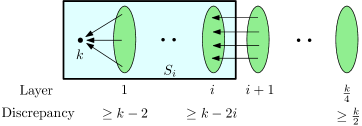
Figure 1: local-search for expanders.

The weak-regularity property was used only in Claim 3.7 above; it is easy to alter the proof to show that $\mathsf{vol}(V\setminus S_{k/4})\geq\nicefrac{{\gamma m}}{{4}}$ even if all but $\nicefrac{{n}}{{7}}$ vertices in $G$ satisfy the weak-regularity property. This proves Theorem 3.3.

Corollary 3.9.

Let $G$ be a $\phi$-expander, such that degree of every vertex, except perhaps a subset of at most $\nicefrac{{n}}{{7}}$ vertices, is at least $2\gamma m/n$. Then the discrepancy of Local-Search is $O\big{(}\frac{\log m}{\phi\gamma}\big{)}$.

The expansion plays a crucial role here: in Section 4 we show that locally-optimum solutions of Local-Search can have large discrepancy for general graphs.

3.3 Dynamic Expander Pruning

In this section we prove Theorem 3.5. We first recall the setup. Suppose we start with a $\phi$-expander $G_{0}=(V_{0},E_{0})$, and at each step $t$ some edge $e_{t}$ is deleted by the adversary (call these primary deletions). The goal is to remove a small portion of the graph so that the remaining portion continues to be, say, a $\phi/6$-expander. Since the graph may may violate the expansion requirement due to deletions, we perform additional secondary deletions at each step to maintain a slightly smaller subgraph $G_{t}=(V_{t},E_{t})$ which is $\nicefrac{{\phi}}{{6}}$-expanding, such that $\{e_{1},\ldots,e_{t}\}\cap E_{t}=\varnothing$. Crucially, the number of secondary deletions is only a factor $\nicefrac{{1}}{{\phi}}$ more than the number of primary deletions until that point. The idea of this greedy expander pruning algorithm is simple: whenever the edge deletion $e_{t}$ creates a sparse cut in $G_{t-1}$, we iteratively remove the smaller side of such a sparse cut from the current graph until we regain expansion. (See Algorithm 3 for the formal definition. Again we assume we can find low-conductance cuts; using an approximation algorithm would lose logarithmic factors.)

Algorithm 3 $\textsc{Prune}(G_{t-1},e_{t})$

Input: Graph $G_{t-1}=(V_{t-1},E_{t-1})$ and an edge $e_{t}\in E_{t-1}$ which gets deleted at this step.
Output: A set of vertices $\Delta P$ that have to be pruned from $G_{t-1}$ to get $G_{t}$.

1:Define $G_{t}$ with edges $E_{t}\leftarrow E_{t-1}\setminus e_{t}$ and vertices $V_{t}\leftarrow V_{t-1}$.

2:$\Delta P\leftarrow\varnothing$.

3:while there is a subset $A\subseteq V_{t}$ with $|E_{t}(A,V_{t}\setminus A)|<(\phi/6)\cdot\mathsf{vol}_{0}(A)$ do

4:     Assume that $A$ is the smaller side of the cut

5:     Remove $A$ from $G_{t}$, i.e., $V_{t}\leftarrow V_{t}\setminus A$, $E_{t}\leftarrow G_{t}[V_{t}\setminus A]$, and $\Delta P\leftarrow\Delta P\cup A$.

6:Return $\Delta P$

For a subset $S\subseteq V_{0}$, let $\mathsf{vol}_{0}(S)$ denote its initial volume in $G_{0}$. Observe that the expansion in line 3 above is measured with respect to $\mathsf{vol}_{0}(A)$, the volume of the set $A$ in $G_{0}$, which is a stronger condition than comparing to the volume in the current graph. Define $P_{t}$ to be the set of vertices pruned in the first $t$ iterations, i.e., $P_{t}=V_{0}\setminus V_{t}$, so that $P_{0}=\varnothing$. We now show that this algorithm maintains a “strong expansion” property at all times (i.e., the expansion property holds with respect to the initial volume $\mathsf{vol}_{0}$).

Proof of Theorem 3.5.

The first property uses that $P_{t}$ is the set of vertices removed in the first $t$ steps. The second property uses the stopping condition of the algorithm, and the fact that $\mathsf{vol}_{0}(\{v\})\geq\delta$ for all vertices.

To prove the final property, let the subsets pruned by the algorithm be $A^{1},A^{2},\ldots,A^{s}$ in the order they are pruned. For an index $\ell$, let $B^{\ell}:=\cup_{\ell^{\prime}=1}^{\ell}A^{\ell^{\prime}}$. Let $E_{t}^{\prime}:=E_{0}\setminus\{e_{1},\ldots,e_{t}\}$. The following claim bounds the number of edges leaving $B^{\ell}$.

Claim 3.10.

If set $A^{\ell}$ is pruned in iteration $t$, then $|E_{t}^{\prime}(B^{\ell},V_{0}-B^{\ell})|\leq\frac{\phi}{6}\mathsf{vol}_{0}(B^{\ell})$. Also, $\mathsf{vol}_{0}(B^{\ell})\leq\mathsf{vol}_{0}(V_{0}\setminus B^{\ell})$.

Before we prove this claim, we use it to prove the third property: note that $|E_{0}(B^{\ell},V_{0}\setminus B^{\ell})|\geq\phi\cdot\mathsf{vol}_{0}(B^{\ell})$ because $G_{0}$ is a $\phi$-expander, and moreover $\mathsf{vol}_{0}(B^{\ell})\leq\mathsf{vol}_{0}(V_{0}\setminus B^{\ell})$ by the second part of Claim 3.10. Moreover, the first part of the claim implies that $|E_{t}^{\prime}(B^{\ell},V_{0}\setminus B^{\ell})|\leq\frac{\phi}{6}\mathsf{vol}_{0}(B^{\ell})$. Since $E_{t}^{\prime}$ changes by at most one edge per deletion, it follows that

$$t~{}\geq~{}|E_{0}(B^{\ell},V_{0}\setminus B^{\ell})|-|E_{t}^{\prime}(B^{\ell},V_{0}\setminus B^{\ell})|\geq\phi\cdot\mathsf{vol}_{0}(B^{\ell})-\frac{\phi}{6}\cdot\mathsf{vol}_{0}(B^{\ell})~{}=~{}\frac{5\phi}{6}\mathsf{vol}_{0}(B^{\ell}).$$ (2)

Since $P_{t}$ is the same as $B^{\ell}$ for some $\ell$, this completes the proof. ∎

Proof of Claim 3.10.

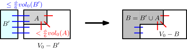
Figure 2: Dynamic expander pruning.

We proceed by induction on $\ell$. When $\ell=0$ this is trivial since $B^{\ell}=\varnothing$. Suppose the claim holds for $B^{\ell-1}$, and we need to prove it for $B^{\ell}=B^{\ell-1}\cup A^{\ell}$. For sake of brevity, we denote $B^{\prime}=B^{\ell-1},B=B^{\ell}$ and $A=A^{\ell}$ (see Figure 2). Any edge in $E_{t}^{\prime}(B,V_{0}\setminus B)$ either lies in $E_{t}^{\prime}(B^{\prime},V_{0}\setminus B)\subseteq E_{t}^{\prime}(B^{\prime},V_{0}\setminus B^{\prime})$ or in $E_{t}^{\prime}(A,V_{0}\setminus B)$. By the induction hypothesis, the former is at most $\frac{\phi}{6}\mathsf{vol}_{0}(B^{\prime})$. The latter, by the condition in line 3, is at most $(\phi/6)\cdot\mathsf{vol}_{0}(A)$. Summing the two, we get $|E_{t}^{\prime}(B,V_{0}\setminus B)|\leq(\phi/6)\mathsf{vol}_{0}(B^{\prime})+(\phi/6)\mathsf{vol}_{0}(A)$, which proves the first part of the claim.

To prove second part of the claim, it suffices to show $\mathsf{vol}_{0}(B)\leq m$. By the induction hypothesis, $\mathsf{vol}_{0}(B^{\prime})\leq m$. Further, by (2) we have $\mathsf{vol}_{0}(B^{\prime})\leq\frac{6t}{5\phi}$. Now two cases arise:

1. $\mathsf{vol}_{0}(B^{\prime})\geq\frac{\phi}{6}\mathsf{vol}_{0}(A)$: In this case,

   $$t~{}\stackrel{{\scriptstyle(\ref{eq:1})}}{{\geq}}~{}\frac{5\phi}{6}\mathsf{vol}_{0}(B^{\prime})~{}\geq~{}\frac{5\phi}{12}\mathsf{vol}_{0}(B^{\prime})+\frac{5\phi^{2}}{72}\mathsf{vol}_{0}(A)~{}\geq~{}\frac{5\phi^{2}}{72}\mathsf{vol}_{0}(B^{\prime}+A)\;=\;\frac{5\phi^{2}}{72}\mathsf{vol}_{0}(B)\enspace.$$

   Since $t\leq\nicefrac{{\phi^{2}m}}{{20}},$ it follows that $\mathsf{vol}_{0}(B)\leq m$.

2. $\mathsf{vol}_{0}(B^{\prime})<\frac{\phi}{6}\mathsf{vol}_{0}(A)$: Consider the cut $(A,V_{0}\setminus B)$. Now,

   $$|E_{0}(A,V_{0}\setminus B)| ~{}=~{}|E_{0}(A,V_{0}\setminus A)|-|E_{0}(A,B^{\prime})|~{}\geq~{}\phi\cdot\mathsf{vol}_{0}(A)-\mathsf{vol}_{0}(B^{\prime})~{}\geq~{}\nicefrac{{5}}{{6}}\cdot\mathsf{vol}_{0}(A).$$

   On the other hand, $A$ is pruned by our algorithm because it is a sparse cut, i.e., $|E^{\prime}_{t}(A,V_{0}\setminus B)|<\frac{\phi}{6}\cdot\mathsf{vol}_{0}(A)$. Therefore, the total number of deletions $t$ is at least $\frac{5\phi}{6}\mathsf{vol}_{0}(A)-\frac{\phi}{6}\mathsf{vol}_{0}(A)=\frac{4\phi}{6}\mathsf{vol}_{0}(A)$. Now we argue as in the first case. We get

   $$t~{}>~{}\frac{3\phi}{6}\mathsf{vol}_{0}(A)+\frac{\phi}{6}\mathsf{vol}_{0}(A)~{}>~{}\frac{3\phi}{6}\mathsf{vol}_{0}(A)+\mathsf{vol}_{0}(B^{\prime})~{}\geq~{}\frac{3\phi}{6}\mathsf{vol}_{0}(B^{\prime}+A)~{}=~{}\frac{\phi}{2}\mathsf{vol}_{0}(B)\enspace.$$

   Since $t\leq\nicefrac{{\phi^{2}m}}{{20}}$, we again get $\mathsf{vol}_{0}(B)\leq m.$ ∎

3.4 Dynamic Local-Search on Expanders with Deletions

In this section we show how to dynamically maintain a locally-optimal orientation of an expander, as parts of it are pruned out over time, thereby proving Theorem 3.6. The algorithm appears as Algorithm 4. We assume that the expander $G_{t-1}$ is maintained by dynamic pruning procedure Prune and satisfies the expansion properties of Theorem 3.5. We also assume that we have a locally optimal orientation ${\vec{G}}_{t-1}$ inductively maintained by Algorithm 4. Then, when the adversary deletes an edge $e_{t}$ and Prune computes a set $\Delta P$ of vertices to remove from $G_{t-1}$ to obtain a graph $G_{t}$, we show how to compute a locally optimal orientation ${\vec{G}}_{t}$ with a bounded number of flips.

Recall that we do this via a potential function argument. For any graph $H$ and current orientation ${\vec{H}}$, the potential of this orientation is $\Phi({\vec{H}}):=\sum_{v\in V(H)}{\mathsf{disc}}(v)^{2}$. Indeed, the main issue is that there could be some vertices in $V_{t-1}\setminus\Delta P$ which are incident to many edges from $\Delta P$. Hence, if we remove $\Delta P$ in one shot, the potential of the residual graph could increase a lot. To resolve this, we replace $\Delta P$ by a set $F$ of an equal number $|\Delta P|$ of fake vertices, and replace all the edges between $V_{t}:=V_{t-1}\setminus\Delta P$ and $\Delta P$ with edges between $V_{t}$ and $F$ in a balanced round-robin manner to preserve the discrepancy of every vertex of $V_{t}$ w.r.t. its discrepancy in ${\vec{G}}_{t-1}$. Due to this balanced way of distributing the edges, we can show that the potential of the fake graph over $V_{t}\cup F$ is no more than that of ${\vec{G}}_{t-1}$, and moreover, even after deleting a subset $F^{\prime}\subseteq F$ of fake vertices, $G_{t}\cup(F\setminus F^{\prime})$ is an expander. These properties motivate running the following algorithm: transition from $G_{t}\cup F$ to $G_{t}$ by removing the fake vertices (and its incident edges) one-by-one, and re-running local search after each deletion.

Algorithm 4 Prune-and-Reorient$({\vec{G}}_{t-1},e_{t},\Delta P)$

Input: Graph $G_{t-1}=(V_{t-1},E_{t-1})$ with orientation ${\vec{G}}_{t-1}$, deleted edge $e_{t}$, and pruned set $\Delta P\subseteq V_{t-1}$.
Output: A low-discrepancy orientation ${\vec{G}}_{t}$ for $G_{t}=(V_{t},E_{t})$ where $V_{t}:=V_{t-1}\setminus\Delta P$ and $E_{t}$ is the subset of $E_{t-1}\setminus\{e_{t}\}$ induced on $V_{t}$.

1:Create fake vertices $F:=\{f_{1},\ldots,f_{N}\}$, where $N=|\Delta P|$, and define $H_{t}:=(V_{t}\cup F,E_{t})$.

2:Let $E^{+}$ be edges in $E_{t-1}(V_{t},\Delta P)\setminus\{e_{t}\}$ oriented from $V_{t}$ to $\Delta P$. Denote $E^{+}=\{e_{1},\ldots,e_{r}\}$, such that all edges incident to a vertex in $V_{t}$ appear consecutively.

3:for $i=1,\ldots,r$ do

4:     For edge $e_{i}=(v_{i},p_{i})\in E^{+}$, add edge $(v_{i},f_{(i\bmod N)+1})$ into $H_{t}$ oriented from $v_{i}$ to $f_{(i\bmod N)+1}$.

5:Repeat above loop for edges $E^{-}$ in $E_{t-1}(V_{t},\Delta P)\setminus\{e_{t}\}$ oriented into $V_{t}$; adds more edges to $H_{t}$.

6:Run Local-Search on $H_{t}$.

7:for each $1\leq j\leq N$ do

8:     Remove vertex $f_{j}$ and incident edges from $H_{t}$.

9:     Run Local-Search on (the current graph) $H_{t}$.

10:Define the final orientation ${\vec{G}}_{t}$ to be the final orientation ${\vec{H}}_{t}$ of $H_{t}$ (there are no fake vertices).

Proof of Theorem 3.6.

Let $H_{t}^{j}$ denote the graph $H_{t}$ after the removal of the fake vertices $f_{1},\ldots,f_{j}$, so that $H_{t}^{0}=H_{t}$. Since $t$ is fixed, we suppress the subscript $t$ for the rest of this discussion.

We begin with some useful claims towards bounding the total number of flips $L_{t}$. Firstly, we show that each of the intermediate graphs is a reasonable expander. The idea is that the pruned set $\Delta P$ is small compared to $V_{t}$, because whenever it becomes sufficiently large, the dynamic expander decomposition algorithm rebuilds the expander and we can charge the recourse to the adversarial deletions. As a result, both the number of fake vertices as well as their volume is substantially smaller than that of the “real” vertices $V_{t}$, and so the expansion properties of $V_{t}$ are approximately retained in each of the intermediate graphs $H^{j}$.

Lemma 3.11.

For each $j\in\{0,\ldots,N\}$, the graph $H^{j}$ is a $\phi/36$-expander.

Proof.

Let $F^{j}:=\{f_{j+1},\ldots,f_{N}\}$ be a suffix of the fake vertices. The vertex set of $H^{j}$ is $W^{j}:=V_{t}\cup F^{j}$. Let $E^{j}$ denote the set of edges in $H^{j}$—these are the union of edges between $V_{t}$, i.e., $E_{t-1}(V_{t})$, and those going between $F^{j}$ and $V_{t}$. Let $S$ be a subset of vertices in $H^{j}$; we need to show that

$$|E^{j}(S,W^{j}\setminus S)|~{}\geq~{}\frac{\phi}{36}\min(\mathsf{vol}^{j}(S),\mathsf{vol}^{j}(W^{j}\setminus S)),$$ (3)

where $\mathsf{vol}^{j}$ denotes the volume with respect to $E^{j}$. Let $\mathsf{vol}_{t}$ denote the volume with respect to the edges $E_{t}=E_{t-1}(V_{t})$. Recall that $\mathsf{vol}_{0}$ denotes the volume with respect to $G_{0}$ (i.e., the expander graph before any deletions were performed).

Without loss of generality, assume that $\mathsf{vol}^{j}(S)\leq\mathsf{vol}^{j}(W^{j}\setminus S)$. Let $S_{r}$ and $S_{f}$ (“real” and “fake”) denote $S\cap A_{t}$ and $S\cap F^{j}$ respectively (see Figure 3).

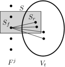
Figure 3: Expansion property of intermediate graphs $W^{j}$.

Claim 3.12.

$\mathsf{vol}_{t}(S_{r})\leq\frac{2}{2-\phi}\cdot\mathsf{vol}_{t}(V_{t}\setminus S_{r})$.

Proof.

We know that $V_{0}=P_{t}\cup V_{t}$. Since $t\leq\phi^{2}m/20$, Theorem 3.5(iii) shows that $\mathsf{vol}_{0}(P_{t})\leq\frac{6}{5\phi}\cdot\frac{\phi^{2}m}{20}\leq\phi m/4$. Therefore, $\mathsf{vol}^{j}(V_{t})$ is at least $2\left(m-\frac{\phi m}{4}\right)=2m-\frac{\phi m}{2}$. Now,

$$\mathsf{vol}^{j}(S_{r})~{}\leq~{}\mathsf{vol}^{j}(S)~{}\leq~{}\mathsf{vol}^{j}(W^{j}\setminus S)~{}\leq~{}\mathsf{vol}^{j}(V_{t}\setminus S_{r})+\mathsf{vol}_{0}(P_{t}).$$

Using $\mathsf{vol}_{0}(P_{t})\leq\phi m/2$, this gives $\mathsf{vol}^{j}(S_{r})-\mathsf{vol}^{j}(V_{t}\setminus S_{r})\leq\phi m/2$. We also know that $\mathsf{vol}^{j}(S_{r})+\mathsf{vol}^{j}(V_{t}\setminus S_{r})=\mathsf{vol}^{j}(V_{t})\geq 2m-\frac{\phi m}{2}$. Eliminating $m$ from these two inequalities gives the claim. ∎

Theorem 3.5 shows that

$$|E^{j}(S_{r},V_{t}\setminus S_{r})|~{}\geq~{}\frac{\phi}{6}\min(\mathsf{vol}_{0}(S_{r}),\mathsf{vol}_{0}(V_{t}\setminus S_{r}))~{}\geq~{}\frac{\phi}{6}\cdot\frac{2-\phi}{2}\cdot\mathsf{vol}^{j}(S_{r})~{}\geq~{}\frac{\phi}{12}\mathsf{vol}^{j}(S_{r}),$$

where the second-last inequality follows from Claim 3.12, and the last inequality uses $\phi\leq 1$.

We now consider two cases:

1. $|E^{j}(S_{f},V_{t}\setminus S_{r})|\geq\mathsf{vol}^{j}(S_{f})/2$: In this case,

   $$|E^{j}(S,W^{j}\setminus S)|~{}\geq~{}|E^{j}(S_{r},V_{t}\setminus S_{r})|+|E^{j}(S_{f},V_{t}\setminus S_{r})|~{}\geq~{}\frac{\phi}{12}\mathsf{vol}^{j}(S_{r})+\frac{1}{2}\mathsf{vol}^{j}(S_{f})~{}\geq~{}\frac{\phi}{12}\mathsf{vol}^{j}(S).$$

2. $|E^{j}(S_{f},V_{t}\setminus S_{r})|\leq\mathsf{vol}^{j}(S_{f})/2$: This implies $\mathsf{vol}^{j}(S_{r})\geq\mathsf{vol}^{j}(S_{f})/2$. Therefore,

   $$|E^{j}(S,W^{j}\setminus S)|~{}\geq~{}|E^{j}(S_{r},V_{t}\setminus S_{r})|~{}\geq~{}\frac{\phi}{12}\mathsf{vol}^{j}(S_{r})~{}=~{}\frac{\phi}{36}(\mathsf{vol}^{j}(S_{r})+2\mathsf{vol}^{j}(S_{r}))~{}\geq~{}\frac{\phi}{36}\mathsf{vol}^{j}(S).$$

Hence the proof of Lemma 3.11 follows. ∎

Next we show that Local-Search gives low discrepancy on the graphs $H^{j}$, even though they may not be weakly-regular.

Lemma 3.13.

For every $j\in\{0,\ldots,N\}$, the discrepancy of $H^{j}$ at a local optimum is $O\big{(}\frac{\log m}{\phi^{2}\gamma}\big{)}$.

Proof.

We apply Corollary 3.9 to $H^{j}$. Lemma 3.11 implies that $H^{j}$ is $\nicefrac{{\phi}}{{36}}$-expander, so it suffices to show that a large fraction of the vertices of $H^{j}$ have large degree.

First of all, since we allow at most $D=\nicefrac{{\phi^{2}m}}{{20}}$ deletions, $\mathsf{vol}_{0}(P_{t})\leq\frac{6}{5\phi}\cdot\frac{\phi^{2}m}{20}=\frac{3\phi m}{50}$ by Theorem 3.5(iii). Using $\gamma$-weak-regularity of $G_{0}$ and $\gamma=\phi/4$ (Theorem 3.4), this implies $|P_{t}|\leq\frac{n}{2m\gamma}\cdot\frac{3\phi m}{50}=\frac{3n}{25}$. So $H^{j}$ has at least $22n/25$ vertices. It follows that $|P_{t}|\leq 3n^{\prime}/22\leq n^{\prime}/7$, where $n^{\prime}$ denotes the number of vertices in $H^{j}$. Now, Theorem 3.5(ii) implies that the degree of any vertex belonging to set $V_{t}$ in the graph $G_{t}$ is at least $\phi\delta/6$, where $\delta\geq 2\gamma m/n$. (This uses that $G_{0}$ is $\gamma$-weakly-regular). Thus, the degree of any vertex in $V_{t}$ in the intermediate graph $H^{j}$ is also at least

$$\frac{\phi\delta}{6}~{}=~{}\frac{2\gamma\phi m}{6n}~{}\geq~{}\frac{22\gamma\phi m^{\prime}}{75n^{\prime}}~{}=~{}\left(\frac{11\gamma\phi}{75}\right)\cdot\frac{2m^{\prime}}{n^{\prime}},$$

where $m^{\prime},n^{\prime}$ denote the number of edges and vertices in $H^{j}$ respectively (since $m^{\prime}\leq m$ and $n^{\prime}\geq 22n/25$ as shown above). The desired result now follows from Corollary 3.9. ∎

We are now ready to conduct the potential-based analysis for bounding the number of flips. We bound the recourse by studying the $\ell_{2}$-potential $\Phi({\vec{H}}^{j}):=\sum_{w\in V(H^{j})}{\mathsf{disc}}(w)^{2}$ as we transition from $G_{t-1}$ to $G_{t}$. Indeed, note that a flip made by local search decreases the potential by at least 1, so the recourse is at most the total increase in the potential. This increase happens during Algorithm 4 when we replace $\Delta P$ by $F$ to get the graph $H_{t}$ (with its resulting orientation), and when we remove the fake vertex $f_{j}$ from $H_{t}^{j-1}$ to get $H_{t}^{j}$ (in line 8). We bound the potential increase during each of these steps.

We give some notation first. Let ${\vec{G}}_{t-1},{\vec{G}}_{t},{\vec{H}}_{t}^{j}$ be the subgraphs $G_{t-1},G_{t},H_{t}^{j}$ oriented after running Local-Search respectively. Let ${\vec{G}}^{\prime}_{t-1}$ denote ${\vec{G}}_{t-1}\setminus\{e_{t}\}$. Recall that $E^{+}$, $E^{-}$ (and therefore $H_{t}$) are defined using edges of ${\vec{G}}^{\prime}_{t-1}$. Let ${{\widetilde{H}_{t}}}$ be the orientation of $H_{t}$ just after we replace $\Delta P$ by $F$ in ${\vec{G}}^{\prime}_{t-1}$ (i.e., before line 6). Similarly let ${{\widetilde{H}^{j}}}$ (we again suppress the subscript $t$ for ease of notation) be the orientation of $H^{j}$ just after we remove $f_{j}$ but before we run Local-Search on it (in line 9). Since edges are added in a round-robin manner between $V_{t}$ and $\Delta P$ in $H_{t}$, there are no parallel edges.

Claim 3.14.

$\Phi({\vec{G}}^{\prime}_{t-1})-\Phi({\vec{G}}_{t-1})$ is at most $O\big{(}\frac{\log m}{\phi^{2}\gamma}\big{)}$.

Proof.

Recall that ${\vec{G}}^{\prime}_{t-1}$ is obtained by removing $e_{t}$ from ${\vec{G}}_{t-1}$. Let $d$ be the maximum discrepancy of a vertex in ${\vec{G}}_{t-1}$. Theorem 3.5 implies that $G_{t-1}$ is an $\Omega(\phi\gamma)$-weakly-regular $\Omega(\phi)$-expander, so Theorem 3.3 implies that the discrepancy $d$ is $O\big{(}\frac{\log m}{\phi^{2}\gamma}\big{)}.$ Hence the removal of $e_{t}$ from ${\vec{G}}_{t-1}$ can increase the potential by at most $2((d+1)^{2}-d^{2})=2(2d+1)=O\big{(}\frac{\log m}{\phi^{2}\gamma}\big{)}$, thus proving the claim. ∎

Next, we show that the potential cannot increase while going from ${\vec{G}}^{\prime}_{t-1}$ to ${{\widetilde{H}_{t}}}$. This uses the fact that we essentially re-distributed all the edges in $E^{+}$ and $E^{-}$ in a balanced round-robin manner.

Claim 3.15.

$\Phi({{\widetilde{H}_{t}}})-\Phi({\vec{G}}^{\prime}_{t-1})\leq 0$.

Proof.

For a given sum $s$ and variables satisfying $\sum_{i=1}^{N}x_{i}=s$, the optimal (w.r.t. $\ell_{2}$ norm) integer assignment of variables has $x_{i}\in\{\lfloor\frac{a_{+}-a_{-}}{N}\rfloor,\lfloor\frac{a_{+}-a_{-}}{N}\rfloor+1\}$ for all $i$ and is unique up to permutations. For our problem, $s=a_{+}-a_{-}$ and the $x_{i}$’s denote the discrepancies of the fake vertices. So it suffices to prove the following:

Claim 3.16.

For each addition of an edge $(v,f)\in(E^{+}\cup E^{-})$ in Algorithm 4, $\exists\,d^{\prime}$ such that just after the addition, $\{{\mathsf{disc}}(f^{\prime})\,|\,f^{\prime}\in F\}\subseteq\{d^{\prime},d^{\prime}+1\}$. In particular, after the addition of all edges, $\{{\mathsf{disc}}(f^{\prime})\,|\,f^{\prime}\in F\}\subseteq\{\lfloor\frac{a_{+}-a_{-}}{N}\rfloor,\lfloor\frac{a_{+}-a_{-}}{N}\rfloor+1\}$.

Proof.

Recall that we first add the edges in $E^{+}$. Since they are added in round robin fashion, the claim is trivially true up to this point. At this point, there will be some prefix of vertices $F^{\prime}\subseteq F$ with discrepancy $d^{\prime}+1$ and the rest have discrepancy $d^{\prime}$. Now consider the addition of edges in $E^{-}$. If $|E^{-}|\leq|F^{\prime}|$, then nodes in $F\setminus F^{\prime}$ remain unchanged and the discrepancy of some nodes in $F^{\prime}$ will become $d^{\prime}$, thus still satisfying the desired property. If $|E^{-}|>|F^{\prime}|$, then after $|F^{\prime}|$ insertions, all nodes will have discrepancy $d^{\prime}$, and after this point, discrepancies decrease by $1$ in a round-robin fashion, thus maintaining the desired property. In particular, after the insertion of all edges, we have $d^{\prime}=\lfloor\frac{a_{+}-a_{-}}{N}\rfloor$. This is because if $\frac{a_{+}-a_{-}}{N}$ is integral, then all vertices in $F$ will have discrepancy $\frac{a_{+}-a_{-}}{N}=\lfloor\frac{a_{+}-a_{-}}{N}\rfloor$ and if $\frac{a_{+}-a_{-}}{N}$ is non-integral, since it is the average discrepancy, it is a convex combination of $d^{\prime}$ and $d^{\prime}+1$, implying $d^{\prime}=\lfloor\frac{a^{-}-a^{+}}{N}\rfloor$. ∎

As explained in the beginning of the proof, the claim immediately implies that $\Phi({{\widetilde{H}_{t}}})\leq\Phi({\vec{G}}^{\prime}_{t-1})$. ∎

Claim 3.17.

For any $j\in\{1,\ldots,N\}$, if $\delta(f_{j})$ is the degree of $f_{j}$ in $H_{t}$, the potential change is

$$\Phi({{\widetilde{H}}}^{j})-\Phi({\vec{H}}^{j-1})~{}\leq~{}O\bigg{(}\frac{\delta(f_{j})\;\log m}{\phi^{2}\gamma}\bigg{)}.$$

Proof.

Let $d$ be the maximum discrepancy of a vertex in ${\vec{H}}^{j-1}$. When we remove the fake vertex $f_{j}$ from ${\vec{H}}^{j-1}$, the discrepancy of the neighbors of $f_{j}$ changes by 1, and so the potential increases by at most $2d\delta(f_{j})$. Lemma 3.13 shows that $d$ is $O\big{(}\frac{\log m}{\phi^{2}\gamma}\big{)}$. ∎

Claims 3.14, 3.15 and 3.17 show that the total increase in the potential due to deletion of $e_{t}$, creation of $H_{t}$ and deletion of a fake vertices is at most $\frac{\log m}{\phi^{2}\gamma}+\frac{\mathsf{vol}_{0}(\Delta P)\log m}{\phi^{2}\gamma}.$ If $L_{t}$ denotes the number of flips performed by Local-Search during Prune-and-Recolor$(G_{t-1},e_{t})$, then

$$\Phi({\vec{G}}_{t})-\Phi({\vec{G}}_{t-1})~{}\leq~{}\left(\frac{\log m}{\phi^{2}\gamma}+\frac{\mathsf{vol}_{0}(\Delta P)\log m}{\phi^{2}\gamma}\right)-L_{t}.$$

This completes the proof of Theorem 3.6. ∎

We end this section by using Theorem 3.6 in an aggregate sense, over a sequence of $t$ adversarial deletions.

Theorem 3.18.

Let $G_{0}=(V_{0},E_{0})$ be a $\gamma$-weakly-regular $\phi$-expander with $m$ edges and $n$ vertices. Suppose at most $D=\nicefrac{{\phi^{2}m}}{{20}}$ edges are deleted adversarially. Then for any $t\leq D$, the total number of edge flips performed by Algorithm 4 during the first $t$ deletions is at most $O\big{(}\frac{\log m}{\phi^{3}\gamma}\cdot t+m\big{)}$.

Proof.

The proof is to simply combine Theorems 3.5 and 3.6 over the sequence of adversarial deletions. Indeed, we can use the facts that the total volume of the pruned set is at most $\mathsf{vol}_{0}(P_{t})\leq 6t/(5\phi)$ along with $\Phi({\vec{G}}_{0})\leq m$ (optimal offline orientation of $G_{0}$ has discrepancy at most $n\leq m$), and $\Phi({\vec{G}}_{t})\geq 0$ to complete the proof. ∎

3.5 Putting Everything Together

We now formally describe our overall algorithms and analyses. To keep track of the internal states of the algorithms, we maintain an internal clock which is initialized at moment $\tau=0$ (but eventually $\tau$ will exceed time $t$). At any moment $\tau$, we maintain a decomposition of the current graph $G_{\mathsf{curr}}(\tau)$ into several subgraphs $\{G_{i}(\tau)\}_{i\geq 0}$, where $G_{i}(\tau)$ is the level-$i$ subgraph of $G_{\mathsf{curr}}(\tau)$. These subgraphs maintain the following invariants:

1. For each moment $\tau$ and level $i$, the graph $G_{i}(\tau)$ has at most $2^{i}$ edges.

2. For every $\tau$ and $i$, subgraph $G_{i}(\tau)$ has a creation moment $\tau_{0}$ which is at most $\tau$. Graph $G_{i}(\tau)$ is a subgraph of $G_{i}(\tau_{0})$, i.e., we only delete edges from this level between $\tau_{0}$ and $\tau$.

3. For each $\tau$ and $i$, we maintain a decomposition of $G_{i}(\tau)$ into subgraphs $G_{i,j}(\tau)$ for $j\geq 1$, such that any vertex appears in at most $\log^{2}n$ of these subgraphs. Moreover, if $\tau_{0}$ is the creation moment of $G_{i}(\tau),$ then $G_{i,j}(\tau_{0})$ is $\gamma$-weakly-regular $\phi$-expander for all $j$, and $G_{i,j}(\tau)$ is a subgraph of $G_{i,j}(\tau_{0})$ for all $j$.

Although not mentioned explicitly in the invariants, the subgraph $G_{i,j}(\tau)$ also has expansion and the weak-regularity properties given by Theorem 3.5: in the notation of this theorem, $G_{i,j}(\tau)=G_{t}$, where $G_{0}$ is the corresponding subgraph at the creation moment $\tau_{0}$ of $G_{i}(\tau)$.

Edge Insertions. We first consider the (easier) case of adversarial edge insertions. The algorithm appears in Algorithm 5. We first insert the edge $e$ into level-$1$. Whenever a level-$j$ subgraph overflows (i.e., has more than $2^{j}$ edges), we empty this level and move all the edges to the subsequent level. If this process stops at level $j$, we build a new expander decomposition of the graph at this level using Theorem 3.4, and also recompute an optimal offline low-discrepancy discrepancy orientation for each expander. As mentioned before, it is easy to optimally orient any graph in the offline setting: we consistently orient the edges of all cycles, to be left with a forest. We can then again orient all the maximal paths between pairs of leaves in a consistent manner, to end up with an orientation where every vertex has discrepancy in $\{-1,0,1\}$. Note that since it is the optimal discrepancy solution, it is also a locally optimal orientation.

Algorithm 5 Insert$(e,\tau)$

Input: Edge $e$ to be inserted in $G_{\mathsf{curr}}(\tau)$.
Output: Graph $G_{\mathsf{curr}}(\tau+1)$ with decomposition into levels.

1:Find the smallest $i$ such that $\{e\}\cup G_{1}(\tau)\cup\cdots\cup G_{i}(\tau)$ has at most $2^{i}$ edges.

2:Set $G_{i^{\prime}}(\tau+1)=\varnothing$ for $i^{\prime}=1,\ldots,i-1$.

3:Set $G_{i^{\prime}}(\tau+1)\leftarrow G_{i^{\prime}}(\tau),$ for all $i^{\prime}>i$ and $G_{i}(\tau+1)\leftarrow\{e\}\cup G_{1}(\tau)\cup\cdots\cup G_{i}(\tau).$

4:Let the expander decomposition of $G_{i}(\tau+1)$ (using Theorem 3.4) return subgraphs $G_{i,j}(\tau+1),j\geq 1$; define their creation moment to be $\tau+1$.

5:Find a discrepancy-at-most-$1$ orientation for each $G_{i,j}(\tau+1),j\geq 1$.

6:$\tau\leftarrow\tau+1$

Edge Deletions. For the case of adversarial edge deletions, when an edge $e$ is deleted from subgraph $G_{i,j}(\tau)$, we first check if $\tfrac{\phi^{2}m_{i,j}}{20}$ edges have been deleted from $G_{i,j}(\tau_{0})$, where $\tau_{0}$ is the creation moment of $G_{i}(\tau)$ and $m_{i,j}$ was the number of edges in $G_{i,j}(\tau_{0})$. If so, we remove the subgraph $G_{i,j}(\tau)$ and re-insert these edges (these are called internal inserts). Otherwise, we run Algorithm 3 on $G_{i,j}(\tau)$ and edge $e$ to get subset $\Delta P$, and then call Algorithm 4 which removes $\Delta P$ (via secondary deletes) and reorients edges of $G_{i,j}(\tau)$. Finally, the edges of $\Delta P$ are re-inserted (causing more internal inserts). The algorithm is shown formally in Algorithm 6.

Algorithm 6 Delete$(e,\tau)$

Input: Edge $e$ to be deleted from $G_{\mathsf{curr}}(\tau)$.
Output: Graph after deletion of edge $e$.

1:Find the level $i$ and index $j$ such that $e$ belongs to $G_{i,j}(\tau).$

2:Let $\tau_{0}\leftarrow$ creation moment of $G_{i}(\tau)$, and $m_{i,j}\leftarrow$ number of edges in $G_{i,j}(\tau_{0})$.

3:Let $T_{i,j}$ be the set of $\tau^{\prime}\in[\tau_{0},\tau]$ at which an adversarial edge deletion happened in $G_{i,j}(\tau^{\prime})$.

4:if $|T_{i,j}|\geq\nicefrac{{\phi^{2}m_{i,j}}}{{20}}$ then

5:     Remove all edges in $G_{i,j}(\tau)$, re-insert all except $e$ one-by-one using Algorithm 5 while incrementing $\tau$.

6:else

7:     $\Delta P\leftarrow\textsc{Prune}(G_{i,j}(\tau),e)$ (see Algorithm 3, where $t=|T_{i,j}|$, and $G_{t-1}=G_{i,j}(\tau)$).

8:     $G_{i,j}(\tau+1)\leftarrow\textsc{Prune-and-Reorient}(G_{i,j}(\tau),e,\Delta P$) (see Algorithm 4) and $\tau\leftarrow\tau+1$.

9:     Reinsert edges of $\Delta P$ except $e$ one-by-one while incrementing $\tau$ using Algorithm 5.

We are now ready to analyze the discrepancy of $G_{\mathsf{curr}}(\tau)$ for all $\tau$, as well as the amortized recourse. We will prove the following quantitative version of Theorem 1.2.

Theorem 3.19 (Main Theorem: Graph Orientation).

Suppose we start with the empty graph on $n$ vertices and it undergoes adversarial edge insertions and deletions. There is an algorithm that maintains discrepancy of $O(\log^{7}n)$ with an amortized recourse of $O(\log^{5}n)$ per update.

Proof.

Firstly, we can assume w.l.o.g. that we never have parallel edges, as we can handle repetitions in the following black-box manner. Let $E$ denote the set of active edges and let $E^{\prime}$ denote the set of active edges in the no-repetitions black-box. For the copies of an edge $e$ in $E$ (call it $T_{e}$), we will maintain the following invariants: (a) if $|T_{e}|$ is even, then $e\notin E^{\prime}$ and half of them are signed $+1$ and, (b) if $|T_{e}|$ is odd, then $e\in E^{\prime}$ and the $1$’s and $-1$’s in $T_{e}$ differ by at most one such that overall the signs add up to $\sigma^{\prime}(e)$. These invariants ensure that the discrepancy for $E$ is equal to that for $E^{\prime}$. To maintain these invariants:

1. If $|T_{e}|$ is even and $e$ is added/deleted in $E$, then call insert procedure with $e$ into $E^{\prime}$ and for each edge $e^{\prime}$ whose orientation changes in $E^{\prime}$, you have to flip exactly one copy in $T_{e^{\prime}}$ to satisfy the invariant.

2. If $|T_{e}|$ is odd and $e$ is added/deleted in $E$, then you have to re-orient at most one of edge in $T_{e}$ to ensure that $+1$’s and $-1$’s are equal in $T_{e}$. Then call delete procedure on $e$ from $E^{\prime}$. Again, for each edge $e^{\prime}$ flipped in $E^{\prime}$, you have to flip exactly one copy in $T_{e^{\prime}}$ to satisfy the invariant.

For the rest of the proof we assume that there are no parallel edges. We first bound the recourse of the algorithm. There are two sources of recourse:

1. While performing a discrepancy-at-most-$1$ orientation in 5 of Insert (Algorithm 5): this could happen due to adversarial insert or internal inserts, i.e., due to lines 5 or 9 in Algorithm 6.

2. During Local-Search performed inside procedure Prune-and-Reorient, called in line 8 of Algorithm 6.

We first bound the number of calls to the Insert procedure. Let $T$ denote the total number of adversarial inserts and deletes.

Claim 3.20.

The total number of calls to Insert procedure is at most $\frac{2T}{\phi^{2}\gamma}.$

Proof.

Clearly, the number of adversarial inserts is at most $T$. First consider the internal inserts caused by line 5 of Algorithm 6. These can be charged to the $\phi^{2}\gamma m_{i,j}$ adversarial deletes in the set $T_{i,j}$. Therefore, the number of such calls to Insert procedure is at most $\frac{T}{\phi^{2}\gamma}.$ Similarly, the number of inserts in line 9 of Algorithm 6 is at most $\mathsf{vol}_{0}(\Delta P)$, the total number of such internal inserts corresponding to a fixed expander graph which undergoes $D^{\prime}\leq D$ adversarial edge deletions is at most $\frac{6D^{\prime}}{5\phi}$ (by Theorem 3.5). Summing over all expanders, this quantity is at most $\frac{6T}{5\phi}$. Thus, the overall number of calls to Insert is at most $\frac{2T}{\phi^{2}\gamma}.$ ∎

We now bound the recourse caused by rebuilding of levels due to insertions.

Claim 3.21.

The total re-orientations due to 5 of Insert is at most $\frac{4T\log m}{\phi^{2}\gamma}$.

Proof.

For a fixed level ${i^{\star}}$, let $T^{\prime}$ be the set of $\tau$ when we call Insert and the index $i$ selected in line 1 in Algorithm 5 happens to be ${i^{\star}}$. For any such moment $\tau$, the total number of edges added to $G_{i}(\tau+1)$ is at most $2^{i^{\star}}$ and at least $2^{{i^{\star}}-1}$. It follows that the number of re-orientations due to 5 of Insert at this moment is also at most $2^{i^{\star}}$. Note that we empty the levels $1,\ldots,{i^{\star}}-1$ at this moment. Therefore, between any two consecutive moments in $T^{\prime}$, we must have inserted at least $2^{{i^{\star}}-1}$ edges (these could be either adversarial or internal inserts). Thus, the total number of re-orientations due to 5 of Insert for all moments in $T^{\prime}$ is at most twice the total number of calls to Insert, which is at most $\frac{2T}{\phi^{2}\gamma}$ (by Claim 3.20).

Since there are at most $\log m$ levels, the desired result follows. ∎

We will next bound the recourse due to local-search steps in the Prune-and-Reorient procedure.

Claim 3.22.

The total number of re-orientations due to Local-Search called in line 6 of Algorithm 4 is $O\left(\frac{T\log n}{\gamma\phi^{3}}\right)$.

Proof.

Consider any particular expander graph $G_{i,j}(\tau_{0})$ created at moment $\tau_{0}$. Consider the calls to the Prune-and-Reorient procedure where the deleted edge belongs to $G_{i,j}(\tau^{\prime})$ for some $\tau^{\prime}\geq\tau_{0}$. We know that $D^{\prime}\leq D$, this inequality could be strict because we may remove all the level $i$ edges at some moment because of line 2 in Algorithm 5. Theorem 3.18 shows that the total number of re-orientations due to Local-Search called in line 6 of Prune-and-Reorient procedure during these $D^{\prime}$ moments is at most (a constant factor of) $\frac{D^{\prime}\log m}{\gamma\phi^{3}}+m_{i,j},$ where $m_{i,j}$ is the number of edges in $G_{i,j}(\tau)$. When we add the above for all expanders, the first term is at most $\frac{T\log m}{\gamma\phi^{3}}$. The second term is the sum over all expanders that get created during the algorithm of the number of edges in the expander. Expanders are created in line 4 of Algorithm 5, and so their total size can be bounded in the same manner as the argument used in the proof of Claim 3.21. Hence this quantity is at most $\frac{4T\log m}{\phi^{2}\gamma}$. ∎

Since we use $\phi,\gamma=\Theta(1/\log n)$, the above results show that the amortized recourse is at most $O\left(\gamma^{-1}\phi^{-3}\log n\right)=O\left(\log n\cdot\log^{3}n\cdot\log n\right)=O(\log^{5}n)$. We now bound the discrepancy of any vertex.

Claim 3.23.

The discrepancy of any vertex is bounded by $O(\log^{7}n)$ at all times.

Proof.

From Lemma 3.13, discrepancy of a vertex in any expander is $O(\phi^{-2}\gamma^{-1}\log m)$, which is $O(\log^{4}n)$ since we use $\gamma,\phi=\Theta(1/\log n)$. Since each vertex appears in at most $O(\log^{3}n)$ expanders, we get that the discrepancy is bounded by $O(\log^{7}n)$ at all times. ∎

This completes the proof of Theorem 3.19. ∎

4 Lower Bounds for Local Search

In this section, we will show that for general vectors and general graphs, typical $\ell_{2}$-potential local search procedures do not guarantee low discrepancy.

4.1 The $\ell_{2}$-Potential for General Vectors

The $\ell_{2}$-potential for a signing $\{\varepsilon_{i}\}$ for vectors $a_{i}$ is $\sum_{j}(\sum_{i}\varepsilon_{i}a_{ij})^{2}=\|S\|^{2}$, where $S:=\sum_{i}\varepsilon_{i}a_{i}$. Hence we are at a local optimum if for each $i$, the potential change $\|S-2\varepsilon_{i}a_{i}\|_{2}-\|S\|_{2}$ due to flipping $a_{i}$ is non-negative. We will show that there exist locally optimal solutions on $T$ vectors with discrepancy $\Omega(\sqrt{T})$.

Consider the following set of vectors in 2 dimensions: $T/2$ vectors of the form $(1,1/\sqrt{T})$ and $T/2$ vectors of the form $(-1,1/\sqrt{T})$ with signing $\varepsilon=\mathbf{1}$. Adding these vectors, we get $S=(0,\sqrt{T})$. Now, for any vector $a$ (w.l.o.g. $a=(1,1/\sqrt{T})$) in the collection,

$$||S-2a||_{2}^{2}-||S||_{2}^{2}~{}=~{}||(-2,\sqrt{T}-\frac{2}{\sqrt{T}})||_{2}^{2}-||(0,\sqrt{T})||_{2}^{2}~{}=~{}4+\left(\sqrt{T}-\frac{2}{\sqrt{T}}\right)^{2}-T~{}=~{}\frac{4}{T}~{}>~{}0.$$

Hence, this is indeed a local optimum and has discrepancy $\sqrt{T}$.

4.2 The $\ell_{2}$-Potential for $\{\pm 1\}$-Vectors

The $\ell_{2}$-potential for a signing $\{\varepsilon_{i}\}$ for $\pm 1$-vectors $a_{i}$ is $\sum_{j}(\sum_{i}\varepsilon_{i}a_{ij})^{2}=\|S\|^{2}$, where $S:=\sum_{i}\varepsilon_{i}a_{i}$. Hence we are at a local optimum if for each $i$, the potential change $\|S-2\varepsilon_{i}a_{i}\|_{2}-\|S\|_{2}$ due to flipping $a_{i}$ is non-negative. Since $\|a_{i}\|_{2}^{2}=n$, the above condition is equivalent to showing

$$S^{\intercal}(\varepsilon_{i}a_{i})\leq n$$ (4)

for all $i$. We can show an $\Omega(2^{n/2})$ locality gap in this case.

Lemma 4.1.

There is a family of instances of $\{\pm 1\}$ vectors, one for each $n$ that is a multiple of $8$, having local optima with discrepancy $\Omega(2^{n/2})$ but global optima having zero discrepancy.

Proof.

We construct a $\{\pm 1\}$ matrix $M$ with $n$ columns and $2\cdot\sum_{i=1}^{n/2}r_{i}$ rows, where $r_{i}$ is set later. We prove that giving signs $\varepsilon=1$ to the rows of this matrix is a local optimum with large discrepancy. Let $S=\boldsymbol{\varepsilon}M$ denote the sum of the rows of $M$. Our construction consists of repeating units, where the $i^{\text{th}}$ repeating unit (for $i=1,\ldots,n/2$) is the following $2\times n$ sub-matrix:

$$\begin{bmatrix}\begin{bmatrix}-1&-1\\ -1&-1\end{bmatrix}\text{ repeated $i-1$ times},\begin{bmatrix}1&1\\ 1&1\end{bmatrix},\begin{bmatrix}1&-1\\ -1&1\end{bmatrix}\text{ repeated $\frac{n}{2}-i$ times}\end{bmatrix}_{2\times n}.$$

This unit is repeated $r_{i}$ times. We will later set $r_{i}$ to an even number, implying that any vector appears an even number of times. Therefore, by signing these even number of copies in an alternating fashion, we get that the global optimum has discrepancy $0$. By construction, $S=(s_{1},s_{1},s_{2},s_{2},...,s_{n/2},s_{n/2})$ for some integers $s_{j}$. Define $\vec{s}:=(s_{1},s_{2},\ldots,s_{n/2})$.

Claim 4.2.

Let $B$ be the $\frac{n}{2}\times\frac{n}{2}$ lower-triangular matrix with $1$s on the diagonal and $-1$s in the lower triangle. Then using $\vec{r}:=(r_{1},\ldots,r_{n/2})^{\intercal}=\frac{n}{4}(B^{-1})^{\intercal}B^{-1}\mathbf{1}$ results in $M$ whose row-sum $S=(s_{1},s_{1},s_{2},s_{2},\ldots,s_{n/2},s_{n/2})$ satisfies $\vec{s}:=(s_{1},s_{2},\ldots,s_{n/2})^{\intercal}=2B^{\intercal}\vec{r}$. Moreover, $\epsilon_{i}=1$ for all $i$ is a local optimum.

Proof.

The row sum $(s_{1},s_{1},s_{2},s_{2},\ldots,s_{n/2},s_{n/2})$ satisfies:

$$2r_{1}-\ldots-2r_{n/2-1}-2r_{n/2} =s_{1}$$

$$\vdots$$

$$2r_{n/2-1}-2r_{n/2} =s_{n/2-1}$$

$$2r_{n/2} =s_{n/2}$$

which implies $\vec{s}=2B^{\intercal}\vec{r}$. Next, we check the condition (4) for local optimality: for any vector $a$ in the $i^{\text{th}}$ repeating unit,

$$\langle S,a\rangle=-2s_{1}-2s_{2}-\ldots-2s_{i-1}+2s_{i}=2(B\vec{s})_{i}=2(B\cdot 2B^{\intercal}\vec{r})_{i}=n.\qed$$

Putting the facts from Claim 4.2 together, the discrepancy vector $\vec{s}=2B^{\intercal}\vec{r}=\frac{n}{2}B^{-1}\mathbf{1}$. We explicitly write down the inverse of the lower-triangular matrix as follows:

$$\begin{bmatrix}1&&&&\\ -1&\ddots&&&\\ \vdots&\ddots&\ddots&&\\ \vdots&&\ddots&\ddots&\\ -1&\cdots&\cdots&-1&1\end{bmatrix}_{k\times k}^{-1}=\begin{bmatrix}1&&&&\\ 1&\ddots&&&\\ 2&\ddots&\ddots&&\\ \vdots&\ddots&\ddots&\ddots&\\ 2^{k-2}&\cdots&2&1&1\end{bmatrix},$$

Using this, we get that $\vec{s}$ has entries of value $\Omega(2^{n/2})$, which proves Lemma 4.1. ∎

Remark 4.3.

Since our example has repetitions, we could try to use this structure to assign opposite signs to these multiple copies, and thereby get low discrepancy. However, it is easy to extend this to avoid repetitions. Since $(r_{1},\ldots,r_{n/2})=\frac{n}{4}(B^{-1})^{\intercal}B^{-1}\mathbf{1}$, the total number of rows $R=\sum_{i}r_{i}$ in our original example is even and at most $2^{4n}$. Take the original matrix $M$, append $2^{4n}-R$ rows of $(1,-1,1,-1,\ldots)$ and $(-1,1,-1,1,\ldots)$ in alternation to obtain a $2^{4n}\times n$ matrix $M^{\prime}$. Moreover, append a $2^{4n}\times 4n$ matrix of all possible $\{\pm 1\}^{4n}$ vectors to the right of $M^{\prime}$ to get the final $2^{4n}\times 5n$ matrix $M^{\prime\prime}$. The row sum is now $S^{\prime\prime}=(S,\mathbf{0}^{4n})$, and any vector in the first $R$ rows continues to satisfy $\langle S^{\prime\prime},a\rangle=n\leq 5n$ by construction. For any vector after that, $\langle S^{\prime\prime},a\rangle=0\leq 5n$, because $\langle(s_{1},s_{1},\ldots,s_{n/2},s_{n/2}),(1,-1,1,-1,\ldots)\rangle=0$. So $M^{\prime\prime}$ has rows in $\{\pm 1\}^{5n}$, and it is a local optimum with discrepancy $\Omega(2^{n/2})$.

4.3 The $\ell_{2}$-Potential for General Graphs

We saw that the local search with the $\ell_{2}$ potential was effective on expanders: however, it fails for general graphs. We now show instances with $n$ vertices and local optima having discrepancy $\Omega(n^{1/3})$.

Lemma 4.4.

There is an infinite family of graph instances with local optima for the $\ell_{2}$-potential having discrepancy $\Omega(n^{1/3})$.

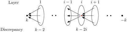
Figure 4: Lower bound of $\Omega(n^{1/3})$ discrepancy for local search on graphs.

Proof.

For even integer $k=\Omega(n^{1/3})$, construct a layered digraph with $k$ layers (see Figure 4). Denote the vertices in layer $i$ by $L_{i}$. For every $u\in L_{i}$ and $v\in L_{i+1}$, add a directed edge from $v$ to $u$. The number of vertices $n_{i}$ in layer $L_{i}$ is chosen so that the root has discrepancy $k$ and each node in $L_{i}$ has discrepancy $k-2i$. Since a node $u\in L_{i}$ has incoming edges from every $v\in L_{i+1}$ and outgoing edges to every $v^{\prime}\in L_{i-1}$, it suffices to have $n_{i+1}-n_{i-1}={\mathsf{disc}}(u)=k-2i$. The base cases are $n_{0}=1$, $n_{1}=k$. Since $k$ is even, this recurrence results in a symmetric instance with a zero-discrepancy layer at the center. There are $k$ layers, and increase in size from $n_{i-1}$ to $n_{i+1}$ is at most $k$. So the total number of nodes (up to constant factors) is at most $k+2k+\ldots+(k)k=(1+2+\ldots+k)k=O(k^{3})$.

Finally, each node in $L_{i}$ has discrepancy equal to $k-2i$ by construction. Since all edges (in the directed graph) are of the form $u\rightarrow v$ with $u\in L_{j},v\in L_{j-1}$ for some $j$, we have that ${\mathsf{disc}}(v)-{\mathsf{disc}}(u)=(k-2(j-1))-(k-2j)=2$, and hence the orientation is indeed a local optimum. ∎

5 Upper-Bounds for Local Search on Unstructured Graphs and Vectors

In Section 3 we saw how local search with the $\ell_{2}$-potential on expander graphs results in small discrepancy; and Section 4 gave strong lower bounds for general graphs, and general collections of vectors. In this section we give an upper bound for general graphs that matches the lower bounds; for vectors, we get an exponential-in-$n$ (but quantitatively weaker) upper bound.

5.1 Local Search Upper Bound of $n^{O(n)}$ for $\{\pm 1\}$ vectors

Let us consider a locally optimal configuration. Without loss of generality, $\varepsilon=1$. For each participating vector $a$, using the fact that $\|a\|_{2}^{2}=n$, we can rewrite the condition $\|S-2a\|_{2}\geq\|S\|_{2}$ as $S^{T}a\leq n$. So for the worst case we are interested in the following program.

$$\max_{a_{1},\ldots,a_{T}\in\{\pm 1\}^{n},\,S=\sum_{i}a_{i}}\|S\|_{\infty}$$

$$\text{s.t. }\langle S,a_{i}\rangle\leq n\,\,\forall i\in[T].$$

We can show that for $\{\pm 1\}$ vectors, discrepancy at a local optimum is bounded by a function of $n$, independent of $T$. Without loss of generality, $S$ has all positive coordinates. For any vector $u\geq 1$,

$$\|S\|_{\infty}\leq\langle S,u\rangle$$

Suppose there is such a $u$ of the form $\sum x_{i}a_{i}$ with $x_{i}\geq 0$, then we will get $\|S\|_{\infty}\leq n\cdot(\sum x_{i})$ since $\langle S,a_{i}\rangle\leq n$. Clearly $x_{i}=1$ is a feasible solution, but instead let us optimize it as follows.

$$\min \textstyle\sum_{i=1}^{T}x_{i}$$

$$x_{i} \geq 0 i=1,\ldots,T T$$ for ( constraints)

$$\textstyle\sum_{i=1}^{T}x_{i}a_{i} \geq 1 n$$ ( constraints)

Let $x^{*}$ be a corner in the feasible region. By definition of a corner, we will have $T$ linearly independent tight constraints at $x^{*}$. Let $n^{\prime}\leq n$ of them be of the second kind and $T-n^{\prime}$ of the first kind. That is, there are $n^{\prime}$ non-zero $x^{*}_{i}$’s. Then we will have $\sum_{i:x^{*}_{i}\neq 0}x^{*}_{i}a^{\prime}_{i}=1$, where $a^{\prime}_{i}$ is obtained from $a_{i}$ by retaining only the $n^{\prime}$ coordinates corresponding to tight constraints. Arranging these $n^{\prime}$-dimensional vectors as columns of a matrix, we get a $n^{\prime}\times n^{\prime}$ matrix $V$ with $V\beta=1$, where $\beta$ is a $n^{\prime}$ dimensional vector containing the nonzero $x^{*}_{i}$’s. $V$ is full rank since if the rows had a non-trivial linear combination giving zero, then using those coefficients for the $n^{\prime}$ type-2 tight constraints will give a vector that is non-zero only at positions $i$ where $x^{*}_{i}=0$. So it is a linear combination of the $T-n^{\prime}$ type 1 tight constraints of the form $x_{i}=0$. This contradicts the linear independence of the tight constraints at a vertex. Hence $V$ is full rank, which implies $\beta=V^{-1}\mathbf{1}$.

Claim 5.1.

The entries of $\beta$ are bounded by $n^{O(n)}$.

Proof.

For a $k\times k$ matrix $M$, $\det(A)=\sum_{\pi\in S_{k}}sign(\pi)m_{1,\pi(1)}m_{2,\pi(2)}...m_{k,\pi(k)}$. Since there are at most $k^{k}$ permutations, any $k\times k$ matrix with $\pm 1$ entries has determinant at most $k^{k}$. We know that $V^{-1}=\frac{adj(V)}{\det(V)}$ and each entry of $adj(V)$ is the determinant of a $(n^{\prime}-1)\times(n^{\prime}-1)$ submatrix of $V$ (i.e., by removing a row and column). Also since $V$ is an invertible $\pm 1$ matrix, $|\det(V)|\geq 1$. Hence we have that entries of $V^{-1}$ are bounded by $(n^{\prime}-1)^{n^{\prime}-1}=O(n^{n})$, and since $\beta=V^{-1}\mathbf{1}$, the entries of $\beta$ are also bounded by $n^{O(n)}$. ∎

Now recall that $\|S\|_{\infty}\leq n\cdot(\sum_{i=1}^{T}\alpha_{i})=n\cdot(\sum_{j=1}^{n^{\prime}}\beta_{j})$ since $\beta$ is a $n^{\prime}$ dimensional vector containing the non-zero $x_{i}$’s. Claim 5.1 implies that this quantity is at most $n\cdot(\sum_{j=1}^{n^{\prime}}n^{O(n)})\leq n\cdot(n^{\prime}\cdot n^{O(n)})=n^{O(n)}$.

5.2 Local Search for General Graphs: Upper Bounds

In this section, we will show upper bounds for a simple variant of Local-Search involving flips along directed paths instead of single edges. We will refer to it by Path-Local-Search with parameter $L$ (Algorithm 7). This is simpler than the method involving expander decompositions (Theorem 3.19), but does not guarantee logarithmic bounds. (In the next section, we show our analysis is tight.)

Algorithm 7 Path-Local-Search

Input: Graph $G=(V,E)$ and an initial partial coloring, Parameter $L$.
Output: Revised orientation which is a local optimum.

1:Arbitrarily direct any undirected edges in $G$.

2:While there exists a directed path $(u_{0},\ldots,u_{l})$ with $l\leq L$ such that ${\mathsf{disc}}(u_{l})>{\mathsf{disc}}(u_{0})+2$, flip all the edges in the directed path.

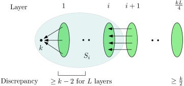
Figure 5: Discrepancy of a local optimum of Path-Local-Search

Theorem 5.2.

Suppose we start with the empty graph on $n$ vertices and it undergoes adversarial edge insertions and deletions such that at any point, the graph does not have multiple edges. Then there is a deterministic algorithm that achieves $O(D)$ discrepancy with $O(\sqrt{n/D})$ amortized recourse for any $\Omega(1)\leq D\leq O(n)$.

Proof.

Recall that Path-Local-Search uses the following rule: if there is a directed path $a\rightarrow b$ of length $\leq L$ such that ${\mathsf{disc}}(b)>{\mathsf{disc}}(a)+2$, then flip all the edges in the path. Let us bound the discrepancy at a local optimum. Let $\vec{G}=(V,\vec{E})$ be the directed graph corresponding to a local optimum. Consider the node $v$ with largest discrepancy $k$; without loss of generality, assume $k\geq 0$. We perform BFS in $\vec{G}$ starting from $v$, following incoming edges at each step. Let $L_{i}$ be the vertices at level $i$ during this BFS, i.e., $L_{i}$ is the set of vertices $w$ for which the shortest path in $\vec{G}$ to $v$ contains $i$ edges. Let $S_{i}$ denote the set of vertices in the first $i$ layers, i.e., $S_{i}:=\bigcup_{i^{\prime}=0}^{i}L_{i^{\prime}}$. The fact that $\vec{G}$ is a local optimum means there are no improving flips, and hence the discrepancy of any vertex in $L_{i}$ is at least $k-2\left(\lfloor\frac{i-1}{L}\rfloor+1\right)$ (see Figure 5). In turn, this implies that there are at least $kL/2$ layers, and the discrepancy of any vertex in $S_{kL/4}$ is at least $k/2$.

We now prove the following claim about the rate at which the number of nodes grows.

Claim 5.3.

Let $n_{i}$ be the number of nodes in layer $i$ for $0\leq i\leq\frac{kL}{4}$, then $|S_{i}|=\sum_{j=0}^{i}n_{j}\geq\frac{i^{2}k}{8}$.

Proof.

By induction. Base case: Trivial since $|S_{0}|=1$. Induction step: Given a directed graph $\vec{G}$ and a subset $X$ of vertices, let $\delta^{-}(X)$ denote the set of incoming edges into $X$ (from $V\setminus X$). Since there are no repeated edges and all edges in $\delta^{-}(S_{i})$ are directed from $L_{i+1}$ to $L_{i}$, we have $|\delta^{-}(S_{i})|\leq n_{i}n_{i+1}$. Since all vertices in $S_{i}$ have discrepancy at least $k/2$, the number of incoming edges $|\delta^{-}(S_{i})|$ must be at least $\frac{k}{2}\cdot|S_{i}|$. Combining the two inequalities, we have $n_{i}n_{i+1}\geq\frac{k}{2}\cdot|S_{i}|.$ Now using this this with the definition of $S_{i+1}$,

$$|S_{i+1}|~{}=~{}|S_{i-1}|+n_{i}+n_{i+1}~{} \geq\frac{(i-1)^{2}k}{8}+2\sqrt{n_{i}n_{i+1}}\quad\text{(induction hypothesis and AM-GM inequality)}$$

$$\geq\frac{(i-1)^{2}k}{8}+2\sqrt{\frac{k}{2}\cdot|S_{i}|}$$

$$\geq\frac{(i-1)^{2}k}{8}+2\sqrt{\frac{k}{2}\cdot\frac{i^{2}k}{8}}\quad\text{(induction hypothesis)}$$

$$\geq\frac{(i-1)^{2}k}{8}+\frac{ik}{2}~{}=~{}\frac{(i+1)^{2}k}{8}\enspace,$$

which completes the proof of Claim 5.3. ∎

Now, Claim 5.3 implies $|S_{kL/4}|\geq(kL/4)^{2}k/8=k^{3}L^{2}/128$. Since we also have $|S_{kL/4}|\leq n$, we get $k\leq O(n^{1/3}/L^{2/3})$. To get the amortized recourse, let us track the $l_{2}$ potential $\Phi=\sum_{u}{\mathsf{disc}}(u)^{2}$, which is initially zero. Before each insertion/deletion, we are at a local optimum, which has a discrepancy of at most $n^{1/3}/L^{2/3}$. So $\Phi$ can change by at most $O(n^{1/3}/L^{2/3})$ when you insert/delete. In each step of local search, $\Phi$ decreases by at least $1$. Since $\Phi\geq 0$, the total number of local search steps is at most $T\cdot\frac{n^{1/3}}{L^{2/3}}$. Since a local search step flips at most $L$ edges, the total recourse is at most $L$ times the number of local search steps. This implies that the amortized recourse is at most $\frac{n^{1/3}}{L^{2/3}}\cdot L=n^{1/3}L^{1/3}$. This proves Theorem 5.2 in the range $\Omega(1)\leq D\leq O(n^{1/3})$.

For the range $\Omega(n^{1/3})\leq D\leq n$, we use the following lemma.

Lemma 5.4.

Perform local search with $L=1$ but perform a step when ${\mathsf{disc}}(v)-{\mathsf{disc}}(u)>\delta$. Then a local optimum has discrepancy at most $n^{1/3}\delta^{2/3}$.

Proof.

Very similar to the previous analysis. There will now be $k/2\delta$ layers, which will imply that total number of vertices is at least $(k/2\delta)^{2}k/8=\Omega(k^{3}/\delta^{2})$. Since this must be at most $n$, this implies that the discrepancy $k=O(n^{1/3}\delta^{2/3})$. The potential drops by at least $\delta$ in each local search step, so amortized recourse will be at most $O(n^{1/3}\delta^{2/3}/\delta)=O(n^{1/3}/\delta^{1/3})$. ∎

This completes the proof of Theorem 5.2. ∎

As an aside, setting $L=1$ and $\delta=2$ in Lemma 5.4 shows the local search in Section 3 achieves $O(n^{1/3})$ discrepancy when performed on general graphs instead of on expanders; this matches the lower bound in Lemma 4.4.

5.3 Tightness of discrepancy bound of Path-Local-Search

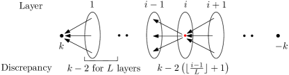
Figure 6: Example showing discrepancy bound at a local optimum of Path-Local-Search in Section 5.2 is tight.

We now provide a family of instances to show that the discrepancy bound for Path-Local-Search given in Section 5.2 is tight. Note that Path-Local-Search with $L=1$ is the same as Local-Search, and so using $L=1$ in the lemma below reproduces the $\Omega(n^{1/3})$ lower bound of Lemma 4.4.

Lemma 5.5.

For Path-Local-Search with parameter $L$, there is a family of instances of increasing size that are each a local optima and have discrepancy $k$ and number of nodes $O(k^{3}L^{2})$.

Proof.

We will construct a layered directed graph with $O(kL)$ layers (see Figure 6). The instance will be symmetric and we will use even $k$ and odd $L$. Let us denote layer $i$ by $L_{i}$. For every $u\in L_{i}$, $v\in L_{i+1}$, there is a directed edge from $v$ to $u$. We will set up the number of vertices $n_{i}$ in each layer so that the root has discrepancy $k$ and each node in $L_{i}$ has discrepancy $k-2\left(\lfloor\frac{i-1}{L}\rfloor+1\right)$. Let us look at a node $u\in L_{i}$. It has incoming edges from every $v\in L_{i+1}$ and has outgoing edges to every $v^{\prime}\in L_{i-1}$. So it suffices to have $n_{i+1}-n_{i-1}={\mathsf{disc}}(u)=k-2\left(\lfloor\frac{i-1}{L}\rfloor+1\right)$. The base cases are $n_{0}=1$, $n_{1}=k$. It is not hard to see that since $k$ is even and $L$ is odd, this recurrence will result in a symmetric instance with an odd number of zero discrepancy layers in the center. There are $O(kL)$ layers and from $n_{i-1}$ to $n_{i+1}$, the increase is at most $k$. So the total number of nodes (up to constant factors) is at most $k+2k+\ldots+(kL)k=(1+2+\ldots+kL)k=O(k^{3}L^{2})$. ∎

One can get tightness for the other side of the tradeoff (Lemma 5.4) by the same idea.

5.4 Local Search for Forests

If we are promised that at each time $t$ the underlying graph is a forest (in the undirected sense), then we can obtain constant discrepancy with logarithmic recourse using the variant of local search that flips along directed paths.

Figure 7: Discrepancy of a local optimum in the forest case

Lemma 5.6.

For forests, performing Path-Local-Search with $L=\log n$ gives $O(1)$ discrepancy and $O(\log n)$ amortized recourse.

Proof.

First, we bound the discrepancy at a local optimum by $3$. For this, suppose for contradiction, the discrepancy (wlog it is positive) is at least 4. Consider the node with discrepancy at least 4 (see Figure 7). It will have a at least 4 incoming edges. Due to local optimum condition with $L=\log n$, each of these children will have discrepancy at least $2$, and therefore will have at least $2$ children. Since $L=\log n$ and forests do not have cycles, we can continue this binary-tree like growth argument till $\log n$ layers. Now the number of nodes will be at least $2^{\log n+1}-1=2n-1$, which is a contradiction. So we get $O(1)$ discrepancy and by the potential based argument as in previous proofs (e.g., Theorem 5.2), we get $O(\log n)$ amortized recourse. ∎

6 Conclusions and Insert-Only Algorithms

In this paper we initiate the study of fully dynamic discrepancy problems, where vectors/edges can both arrive or depart at each time step, and the algorithm must always maintain a low-discrepancy signing. Prior algorithms for online discrepancy could only handle arrivals, and that too only for an oblivious adversary. We obtain near-optimal discrepancy bounds for both the edge-orientation and the vector balancing cases. We achieve the former in near-optimal $\tilde{O}(1)$ amortized recourse, and the latter in ${O}(n)$ amortized recourse (which is exponentially better in $T$ than the naive algorithm which recolors after each update).

The main open question left by our work is whether we can achieve near-optimal discrepancy for vector balancing in $\tilde{O}(1)$ amortized recourse per update. If true, this would imply our edge-orientation results as a special case.

Open Problem 6.1.

For fully-dynamic vector balancing with vectors of $\ell_{2}$ length at most $1$ arriving or departing, can we achieve $\operatorname{poly}\!\log(nT)$ discrepancy in $\operatorname{poly}\!\log(nT)$ amortized recourse per update?

Currently, we don’t know how to achieve near-optimal discrepancy even using $o(n)$ amortized recourse. However, in the case of insertions only (i.e., no departures), we can answer the above question affirmatively using the following Dyadic Resigning algorithm. Note that prior works, e.g. [ALS21, LSS21], could only achieve this against an oblivious adversary.

The Dyadic Resigning algorithm is simple: when the $t^{th}$ vector arrives, let $\ell$ be the largest power of $2$ that divides $t$. Use any offline algorithm $\mathcal{A}$ to construct a fresh signing of the most recently arrived $2^{\ell}$ vectors.

Theorem 6.2.

For any sequence of $T$ adaptive inserts, suppose that an offline algorithm $\mathcal{A}$ can produce a signing of discrepancy at most $D$ when given any subset of these vectors. Then the Dyadic Resigning algorithm achieves at each timestep $t\leq T$ discrepancy at most $D\lceil\log_{2}t\rceil$. Moreover, each vector is assigned a new sign at most $\lceil\log_{2}T\rceil$ times.

Proof.

Let $t=2^{a_{1}}+2^{a_{2}}+\ldots+2^{a_{s}}$, where $a_{1}>a_{2}>\ldots>a_{s}\geq 0$. Let $\tau_{i}=\sum_{j\leq i}2^{a_{j}}$. To prove the discrepancy bound, the main observation is that at each timestep $t$, the current signing consists of the output of $\mathcal{A}$ on $\lceil\log_{2}t\rceil$ different subintervals of the input sequence: $\{v_{1},\ldots,v_{\tau_{1}}\}$, $\{v_{\tau_{1}+1},\ldots,v_{\tau_{2}}\}$, all the way down to $\{v_{\tau_{s-1}+1},\ldots,v_{\tau_{s}}=v_{t}\}$. (This can be proved using an inductive argument.) The discrepancy for each of these logarithmically-many is at most $D$, by our assumption on the algorithm $\mathcal{A}$, which proves the first claim. The second claim uses that each time a vector is given a new sign, it belongs to an subinterval of twice the length; this can happen only $O(\log T)$ times. ∎

Using the algorithm of [Ban98, BDG16] gives us the following result.

Corollary 6.3.

There is an algorithm for the insert-only setting that ensures a discrepancy of $O(\sqrt{\log n}\log T)$ for any sequence of vectors of $\ell_{2}$ length at most $1$ (and hence discrepancy of $O(\sqrt{s\log n}\log T)$ for any sequence of $s$-sparse vectors with entries in $[-1,1]$) in $O(\log T)$ amortized recourse per update.

Another interesting future direction is to get near-optimal discrepancy for small worst-case recourse per update (instead of amortized recourse). E.g., in the setting of 6.1, can we achieve $\tilde{O}(1)$ discrepancy in $\tilde{O}(1)$ worst-case recourse per update? It will also be interesting to improve Corollary 6.3 to get $O(1)$ amortized recourse per update, or to even get $O(1)$ worst-case recourse per update.

Appendix A Missing Details of Section 2

We first prove Lemma 2.2, which is restated below.

See 2.2

Proof.

The proof is by induction on the height of $v$: we also add to the induction hypothesis the statement that all the indices $i\in P_{v}$ such that $-1<y^{v}_{i}<1,$ belong to $F_{v}$. For a leaf node, the set $F=P_{j}$, and so using line 7, we see that $\sum_{i\in P_{j}}y^{\prime}_{i}a_{i}=0$. Since $y^{v}_{i}=y^{\prime}_{i}$ for all $i\in P_{j}$, the invariant (I1) follows. Invariant (I2) holds because of Lemma 2.1.

Now suppose $v$ is an internal node and assume that the induction hypothesis holds for its children $v_{L}$ and $v_{R}$. Since the assignment $x$ just combines $y^{v_{L}}$ and $y^{v_{R}}$ (line 5), it follows from induction hypothesis that $\sum_{i\in P_{v}}x_{i}a_{i}=0.$ We ensure in line 5 that $\sum_{i\in F}y^{\prime}_{i}a_{i}=\sum_{i\in F}a_{i}x_{i}.$ Therefore,

$$\sum_{i\in P_{v}}y^{v}_{i}a_{i}=\sum_{i\in F}y^{\prime}_{i}a_{i}+\sum_{i\in P_{v}\setminus F}x_{i}a_{i}=\sum_{i\in P_{v}}x_{i}a_{i}=0.$$

This proves that (I1) is satisfied for $y^{v}$. For property (I2), first observe that if $i\notin F$, then $x_{i}\in\{-1,+1\}$ by induction hypothesis, and so $y^{v}_{i}=x_{i}\in\{-1,+1\}$ as well. For the indices $i\in F$, at most $n$ of these satisfy $y^{\prime}_{i}\in(-1,+1)$ (by Lemma 2.1) and so all the variables $y^{v}_{i},i\notin F_{v}$ are either $+1$ or $-1$. ∎

We now give details of the procedure DBGUpdate in Algorithm 8. When a vector $a_{h}$ changes to $a_{h}^{new}$, we only run the algorithm in Lemma 2.1 for the ancestors of the leaf $j$ in $\mathcal{T}$ for which $h\in P_{j}$. We now show that this procedure has the desired properties:

Claim A.1.

Suppose the assignment $y^{old}$ satisfies the following properties for every node $v$: (i) $\sum_{i\in P_{v}}y^{old}_{i}a_{i}=0$, and (ii) there are at most $n$ indices $i\in P_{v}$ for which $-1<y^{old}_{i}<+1$. Then the assignment $y^{r}$, where $r$ is the root node, returned by ${\textsc{DBGUpdate}}(r,y^{old},h,a_{h}^{new})$ also satisfies these properties for every node $v$ (with $a_{h}$ replaced by $a_{h}^{new}$). Further $y^{r}$ and $y^{old}$ differ in at most $O(n\log T)$ coordinates.

Algorithm 8 Distributed-Bárány-Grinberg Update: ${\textsc{DBGUpdate}}(v,y^{old},h,a_{h}^{new})$

Input: A node $v$ of $\mathcal{T}$, assignment $y^{old}$ satisfying (I1) and (I2), an index $j\in P_{v}$ where the corresponding vector $a_{j}$ changes to $a_{j}^{new}$.
Output: $(y^{v},F_{v})$: an assignment $y^{v}_{i}\in[-1,1]$ for each $i\in P_{v}$, and $F_{v}\subseteq P_{v}$ is the index set of “fractionally” signed vectors, i.e., indices $i$ such that $-1<y^{v}_{i}<1$.

1:if $v$ is not a leaf then

2:     Let $v_{L}$ and $v_{R}$ be the left and the right children of $v$ respectively.

3:     Let $\ell\in\{L,R\}$ be such that $j\in P_{v_{\ell}}$ and $\ell^{\prime}$ denote $\{L,R\}\setminus\{\ell\}$.

4:     $(y^{v_{\ell}},F_{v_{\ell}})\leftarrow{\textsc{DBGUpdate}}(a_{\ell},y^{old},j,a_{j}^{new}),$ and $F_{v_{\ell^{\prime}}}:=\{i\in P_{v_{\ell^{\prime}}}\mid-1<y^{old}_{i}<1\}.$

5:     Define $F:=F_{v_{\ell}}\cup F_{v_{\ell^{\prime}}}$, $x_{i}:=y^{v_{\ell}}_{i}$ for all $i\in P_{v_{\ell}},x_{i}:=y^{old}_{i}$ for all $i\in P_{v_{\ell^{\prime}}}$.

6:else

7:     Define $F:=P_{v},x_{i}=0$ for all $i\in P_{v}$.

8:Using Lemma 2.1 find a vector $y^{\prime}\in[-1,1]^{|F|}$ such that (i) $A_{F}\cdot y^{\prime}=A_{F}\cdot x|_{F}$, (ii) there are at most $n$ indices, call it $F_{v}\subseteq F$, such that $-1<y_{i}^{\prime}<1$ (note that if $h\in F$, then column $h$ of $A_{F}$ is $a_{h}^{new}$).

9:Define $y^{v}_{i}=x_{i}$ for $i\in P_{v}\setminus F$ and $y^{v}_{i}=y^{\prime}_{i}$ for $i\in F$.

10:Return $(y^{v},F_{v})$.

Proof.

Let the index $h$ belong to $P_{j}$, where $j$ is a leaf node in $\mathcal{T}$. Let $w_{0}=j,w_{1},w_{2},\ldots,w_{H}=r,$ be the path from $j$ to the root $r$ of $\mathcal{T}$. We prove the following by induction on $\ell$. The assignment $(y^{w_{\ell}},F_{v_{\ell}})$ returned by ${\textsc{DBGUpdate}}(w_{\ell},y^{old},h,a_{h}^{new})$ has the following properties: (i) $\sum_{i\in P_{w_{\ell}}}y^{w_{\ell}}_{i}a_{i}=0$, (ii) If $-1<y_{i}<1$ for some $i\in P_{w_{\ell}}$, then $i\in F_{w_{\ell}}$, (iii) $y^{old}|_{P_{w_{\ell}}}$ and $y^{w_{\ell}}$ differ in at most $2n(\ell+1)$ coordinates.

The base case when $\ell=0$ follows easily because of line 8 and Lemma 2.1. Now suppose the induction hypothesis is true for $\ell-1$. Assume wlog that $w_{\ell-1}$ is the left child of $w_{\ell}$ and $w^{\prime}$ be the right child of $w_{\ell}$. By induction hypothesis and property of $y^{old}$, we see that (here $x$ is the assignment defined during DBGUpdate for $w_{\ell}$):

$$\sum_{i\in P_{w_{\ell}}}x_{i}a_{i}=\sum_{i\in P_{w_{\ell-1}}}y^{w_{\ell-1}}_{i}a_{i}+\sum_{i\in P_{w^{\prime}}}y^{old}_{i}a_{i}=0.$$

This proves property (i). Property (ii) can be shown similarly. Again, it follows from induction hypothesis and the property of $y^{old}$ that $|F|\leq 2n$, and so (i) $x$ and $y^{w_{\ell}}$ differ in at most $2n$ coordinates, and (ii) $y^{old}|_{P_{w_{\ell}}}$ and $x$ differ in at most $2n\ell$ coordinates. This implies property (iii). ∎

Corollary A.2.

The amortized recourse during a phase of the DBGUpdate algorithm is $O(n\log N)$.

Proof.

When a phase begins, we run Algorithm 1 to ensure that the assignment $y$ satisfies the conditions stated in Claim A.1 (for the assignment $y^{old}$). Using this result, we see that after each update operation, these conditions continue to be satisfied. Therefore, Claim A.1 shows that the recourse encountered after each update operation is $O(n\log N)$. ∎

References

- [AAG+19] Amir Abboud, Raghavendra Addanki, Fabrizio Grandoni, Debmalya Panigrahi, and Barna Saha. Dynamic set cover: improved algorithms and lower bounds. In Proceedings of the 51st Annual ACM SIGACT Symposium on Theory of Computing, pages 114–125, 2019.
- [AAN+98] Miklos Ajtai, James Aspnes, Moni Naor, Yuval Rabani, Leonard J Schulman, and Orli Waarts. Fairness in scheduling. Journal of Algorithms, 29(2):306–357, 1998.
- [AGZ99] Matthew Andrews, Michel X Goemans, and Lisa Zhang. Improved bounds for on-line load balancing. Algorithmica, 23(4):278–301, 1999.
- [ALS21] Ryan Alweiss, Yang P. Liu, and Mehtaab Sawhney. Discrepancy minimization via a self-balancing walk. In Proceedings of STOC, 2021.
- [Ban98] Wojciech Banaszczyk. Balancing vectors and Gaussian measures of -dimensional convex bodies. Random Struct. Algorithms, 12(4):351–360, 1998.
- [Ban10] Nikhil Bansal. Constructive Algorithms for Discrepancy Minimization. In Proceedings of FOCS 2010, pages 3–10, 2010.
- [BCH17] Sayan Bhattacharya, Deeparnab Chakrabarty, and Monika Henzinger. Deterministic fully dynamic approximate vertex cover and fractional matching in amortized update time. In International Conference on Integer Programming and Combinatorial Optimization, pages 86–98. Springer, 2017.
- [BDG16] Nikhil Bansal, Daniel Dadush, and Shashwat Garg. An algorithm for komlós conjecture matching banaszczyk’s bound. In Proceedings of FOCS 2016, pages 788–799, 2016.
- [BDGL19] Nikhil Bansal, Daniel Dadush, Shashwat Garg, and Shachar Lovett. The Gram-Schmidt walk: A cure for the Banaszczyk blues. Theory Comput., 15:1–27, 2019.
- [Bec81] József Beck. Balanced two-colorings of finite sets in the square I. Combinatorica, 1(4):327–335, 1981.
- [BF81] József Beck and Tibor Fiala. “Integer-making” theorems. Discrete Appl. Math., 3(1):1–8, 1981.
- [BF99] Gerth Stø lting Brodal and Rolf Fagerberg. Dynamic representations of sparse graphs. In Algorithms and data structures (Vancouver, BC, 1999), volume 1663 of Lecture Notes in Comput. Sci., pages 342–351. Springer, Berlin, 1999.
- [BG81] Imre Bárány and Victor S Grinberg. On some combinatorial questions in finite-dimensional spaces. Linear Algebra and its Applications, 41:1–9, 1981.
- [BHI18] Sayan Bhattacharya, Monika Henzinger, and Giuseppe F. Italiano. Deterministic fully dynamic data structures for vertex cover and matching. SIAM Journal on Computing, 47(3):859–887, 2018.
- [BHN19] Sayan Bhattacharya, Monika Henzinger, and Danupon Nanongkai. A New Deterministic Algorithm for Dynamic Set Cover. In 2019 IEEE 60th Annual Symposium on Foundations of Computer Science (FOCS), pages 406–423. IEEE, 2019.
- [BHNW20] Sayan Bhattacharya, Monika Henzinger, Danupon Nanongkai, and Xiaowei Wu. An Improved Algorithm for Dynamic Set Cover. arXiv preprint arXiv:2002.11171, 2020.
- [BJM+21] Nikhil Bansal, Haotian Jiang, Raghu Meka, Sahil Singla, and Makrand Sinha. Online discrepancy minimization for stochastic arrivals. In Proceedings of SODA, pages 2842–2861, 2021.
- [BJSS20] Nikhil Bansal, Haotian Jiang, Sahil Singla, and Makrand Sinha. Online vector balancing and geometric discrepancy. In Proceedings of STOC, pages 1139–1152, 2020.
- [BK19] Sayan Bhattacharya and Janardhan Kulkarni. Deterministically Maintaining a -Approximate Minimum Vertex Cover in Amortized Update Time. In Proceedings of the Thirtieth Annual ACM-SIAM Symposium on Discrete Algorithms, pages 1872–1885. SIAM, 2019.
- [BLSZ14] Bartlomiej Bosek, Dariusz Leniowski, Piotr Sankowski, and Anna Zych. Online bipartite matching in offline time. In 2014 IEEE 55th Annual Symposium on Foundations of Computer Science, pages 384–393. IEEE, 2014.
- [BS20] Nikhil Bansal and Joel H. Spencer. On-line balancing of random inputs. Random Struct. Algorithms, 57(4):879–891, 2020.
- [BvdBG+20] Aaron Bernstein, Jan van den Brand, Maximilian Probst Gutenberg, Danupon Nanongkai, Thatchaphol Saranurak, Aaron Sidford, and He Sun. Fully-dynamic graph sparsifiers against an adaptive adversary. CoRR, abs/2004.08432, 2020.
- [Bá79] I Bárány. On a class of balancing games. Journal of Combinatorial Theory, Series A, 26(2):115–126, 1979.
- [CAHP+19] Vincent Cohen-Addad, Niklas Oskar D Hjuler, Nikos Parotsidis, David Saulpic, and Chris Schwiegelshohn. Fully Dynamic Consistent Facility Location. In Advances in Neural Information Processing Systems, pages 3250–3260, 2019.
- [CDKL09] Kamalika Chaudhuri, Constantinos Daskalakis, Robert D. Kleinberg, and Henry Lin. Online bipartite perfect matching with augmentations. In IEEE INFOCOM 2009, pages 1044–1052. IEEE, 2009.
- [Cha01] Bernard Chazelle. The discrepancy method: randomness and complexity. Cambridge University Press, 2001.
- [EL14] Leah Epstein and Asaf Levin. Robust algorithms for preemptive scheduling. Algorithmica, 69(1):26–57, 2014.
- [FW83] Ronald Fagin and John H. Williams. A fair carpool scheduling algorithm. IBM J. Res. Dev., 27(2):133–139, March 1983.
- [GGK16] Albert Gu, Anupam Gupta, and Amit Kumar. The power of deferral: maintaining a constant-competitive Steiner tree online. SIAM Journal on Computing, 45(1):1–28, 2016.
- [Gia97] Apostolos A Giannopoulos. On some vector balancing problems. Studia Mathematica, 122(3):225–234, 1997.
- [GK14] Anupam Gupta and Amit Kumar. Online Steiner tree with deletions. In Proceedings of the twenty-fifth annual ACM-SIAM symposium on Discrete algorithms, pages 455–467. SIAM, 2014.
- [GKKP17] Anupam Gupta, Ravishankar Krishnaswamy, Amit Kumar, and Debmalya Panigrahi. Online and Dynamic Algorithms for Set Cover. In Proceedings of the 49th Annual ACM SIGACT Symposium on Theory of Computing, STOC 2017, pages 537–550, New York, NY, USA, 2017. ACM.
- [GKKS20] Anupam Gupta, Ravishankar Krishnaswamy, Amit Kumar, and Sahil Singla. Online carpooling using expander decompositions. In Proceedings of FSTTCS, pages 23:1–23:14, 2020.
- [GKKV95] Edward F Grove, Ming-Yang Kao, P. Krishnan, and Jeffrey Scott Vitter. Online perfect matching and mobile computing. In Workshop on Algorithms and Data Structures, pages 194–205. Springer, 1995.
- [GKLX20] Xiangyu Guo, Janardhan Kulkarni, Shi Li, and Jiayi Xian. The Power of Recourse: Better Algorithms for Facility Location in Online and Dynamic Models. arXiv preprint arXiv:2002.10658, 2020.
- [GKS14] Anupam Gupta, Amit Kumar, and Cliff Stein. Maintaining assignments online: Matching, scheduling, and flows. In Proceedings of the twenty-fifth annual ACM-SIAM symposium on Discrete algorithms, pages 468–479. SIAM, 2014.
- [IW91] Makoto Imase and Bernard M Waxman. Dynamic Steiner tree problem. SIAM Journal on Discrete Mathematics, 4(3):369–384, 1991.
- [KKPS14] Tsvi Kopelowitz, Robert Krauthgamer, Ely Porat, and Shay Solomon. Orienting fully dynamic graphs with worst-case time bounds. In Automata, languages, and programming. Part II, volume 8573 of Lecture Notes in Comput. Sci., pages 532–543. Springer, Heidelberg, 2014.
- [Kow07] Ł ukasz Kowalik. Adjacency queries in dynamic sparse graphs. Inform. Process. Lett., 102(5):191–195, 2007.
- [LM15] Shachar Lovett and Raghu Meka. Constructive Discrepancy Minimization by Walking on the Edges. SIAM J. Comput., 44(5):1573–1582, 2015.
- [ŁOP+15] Jakub Łacki, Jakub Oćwieja, Marcin Pilipczuk, Piotr Sankowski, and Anna Zych. The power of dynamic distance oracles: Efficient dynamic algorithms for the Steiner tree. In Proceedings of the forty-seventh annual ACM symposium on Theory of computing, pages 11–20, 2015.
- [LSS21] Yang P. Liu, Ashwin Sah, and Mehtaab Sawhney. A gaussian fixed point random walk. CoRR, abs/2104.07009, 2021.
- [Mat09] Jiří Matousek. Geometric discrepancy: An illustrated guide, volume 18. Springer Science & Business Media, 2009.
- [PW93] Steven Phillips and Jeffery Westbrook. Online load balancing and network flow. In Proceedings of the twenty-fifth annual ACM symposium on Theory of computing, pages 402–411, 1993.
- [Rot14] Thomas Rothvoß. Constructive Discrepancy Minimization for Convex Sets. In Proceedings of FOCS 2014, pages 140–145, 2014.
- [Spe77] Joel Spencer. Balancing games. Journal of Combinatorial Theory, Series B, 23(1):68–74, 1977.
- [Spe85] Joel Spencer. Six standard deviations suffice. Trans. Am. Math. Soc., 289(2):679–706, 1985.
- [SSS09] Peter Sanders, Naveen Sivadasan, and Martin Skutella. Online scheduling with bounded migration. Mathematics of Operations Research, 34(2):481–498, 2009.
- [ST04] Daniel A. Spielman and Shang-Hua Teng. Nearly-linear time algorithms for graph partitioning, graph sparsification, and solving linear systems. In Proceedings of the 36th Annual ACM Symposium on Theory of Computing, Chicago, IL, USA, June 13-16, 2004, pages 81–90, 2004.
- [SV10] Martin Skutella and José Verschae. A robust PTAS for machine covering and packing. In European Symposium on Algorithms, pages 36–47. Springer, 2010.
- [SW19] Thatchaphol Saranurak and Di Wang. Expander decomposition and pruning: Faster, stronger, and simpler. In Proceedings of SODA, pages 2616–2635, 2019.
- [Wes00] Jeffery Westbrook. Load balancing for response time. Journal of Algorithms, 35(1):1–16, 2000.