Power-law fluctuations near critical point in semiconductor lasers with delayed feedback

Abstract

Since the analogy between laser oscillation and second-order phase transition was indicated in the 1970s, dynamical fluctuations on lasing threshold inherent in critical phenomena have gained significant interest. Here, we numerically and experimentally demonstrate that a semiconductor laser subject to delayed optical feedback can exhibit unusual large intensity fluctuations characterized by power-law distributions. Such an intensity fluctuation consists of distinct intermittent bursts of light intensity, whose peak values attain tens of times the intensity of the maximum gain mode. This burst behavior emerges when a laser with a long time delay (over $100\text{\,}\mathrm{n}\mathrm{s}$) and an optimal feedback strength operates around the lasing threshold. The intensity and waiting time statistics follow power-law-like distributions. This implies the emergence of nonequilibrium critical phenomena, namely self-organized criticality. In addition to numerical results, we report experimental results that suggest the power-law intensity dynamics in a semiconductor laser with delayed feedback.

I Introduction

Laser oscillation has gained interest in the areas of theoretical physics as well as engineering application since the analogy between laser oscillation and second-order phase transition was indicated by DeGiorgio and Scully and Graham and Haken DeGiorgio and Scully (1970); Graham and Haken (1970). The analogy to the second-order phase transition has inspired significant interest not just in the transition of a macroscopic quantity, i.e., the onset of laser oscillation, but also its fluctuation around the lasing threshold, which is regarded as a critical point Rice and Carmichael (1994); Kuo et al. (2012); Basak et al. (2016); Wang et al. (2017, 2020). However, despite many studies on this fluctuation of light intensity, scale-invariant fluctuations expected from the context of equilibrium critical phenomena have not been reported.

After nearly two decades of the pioneering works pointing out the analogy, a new concept to understand the scale-invariant fluctuation in nonequilibrium systems, so-called self-organized criticality (SOC), was proposed by Bak, Tang, and Wiesenfeld Bak et al. (1987, 1988) independently of the analogy. SOC is a phenomenon that a dissipative system spontaneously organizes itself to a critical state that is characterized by scale-invariant statistics. That is, a dynamical quantity, $s$, such as the energy released from a dissipative system at one time, the duration, and waiting time of the energy release events follows a power-law distribution:

$$P(s)\propto s^{-\beta}$$ (1)

where $\beta$ is a characteristic exponent Bak et al. (1987, 1988); Jensen (1998); Sornette (2006); Aschwanden (2011). Power-law distributions, which are generalized as Lévy’s stable distributions, have a scale-invariant feature because their mean, variance, and higher order of moments cannot be determined mathematically under a certain condition of the exponent and the upper bound of $s$ Sornette (2006). Thus, dissipation phenomena characterized by the statistical distribution provide substantially large fluctuation and intermittency in their energy dissipation. Such a statistical feature can be found in various natural phenomena and physical systems, e.g., solar flares Aschwanden (2011), earthquakes Omori (1894); Utsu (1969), plasticity Miguel et al. (2001); Niiyama and Shimokawa (2015), sandpiles Bak et al. (1987, 1988), magnetization Durin and Zapperi (2000), and superconductors Field et al. (1995); Jensen (1998). It is considered that the emergence of SOC requires several conditions for a system that stores the energy injected by external driving Jensen (1998): (i) the system dissipates the stored energy through multiple energy-release processes. (ii) the processes interact with each other, and (iii) the processes have threshold values for activation, and (iv) the rate of energy injection into the system is sufficiently slower than that of the energy-release processes.

Interestingly, laser systems appear to satisfy these conditions partly. Evidently, lasers dissipate stored energy and have a threshold value for oscillation. Pumping power, i.e., the rate of energy injection, is able to be controlled as small as possible; thus, the rate can be sufficiently slower than the energy-release rate through the light emission in a low pumping power condition. However, it is unclear whether (i) the multiplicity of the release processes and (ii) their interaction are realized in ordinary lasers, where the multiplicity and the interaction can be introduced by the dimensionality of a system. In these aspects, delayed feedback is likely to play a key role. As is well known, lasers with delayed feedback can be considered as a high-dimensional dynamical system in terms of the spacetime representation; delay systems can be expressed as a spatially expended system Ikeda and Matsumoto (1987); Arecchi et al. (1992); Giacomelli and Politi (1996); Uchida (2012); Erneux et al. (2017). In this representation, numerous independent elements, the so-called virtual nodes that correspond to many degrees of freedom, interact with themselves in a time domain. Hence, delayed feedback can provide multiplicity of the processes and their interactions to the system through high dimensionality.

The delayed feedback also provides a wide variety of dynamical behaviors with laser systems Uchida (2012); Ohtsubo (2012); Erneux et al. (2017). For instance, external light injection with a time delay can cause regular sequential pulsation in a short time scale, the so-called rapid pulse packages (RPPs) Heil et al. (2001), and irregular behaviors, known as optical turbulence, under a strong optical feedback condition Ikeda et al. (1980). Low pump-current conditions near the lasing threshold yield a complex fluctuation, called low-frequency fluctuations (LFF), consisting of sub-nanosecond intensity pulses and regular intensity drops with a longer time scale Fischer et al. (1996); Heil et al. (1998); Ohtsubo (2012). Temporal fluctuations of intermittent pulsation in similar low pumping-power conditions have been investigated and analyzed in terms of intermittent dynamics and extreme events Reinoso et al. (2013); Bosco et al. (2013); Choi et al. (2016); Bosco et al. (2017); Barbosa et al. (2019). In addition, the existence of virtual nodes and their interplay have been used for delay-based computing Appeltant et al. (2011); Larger et al. (2017).

The above similarity to the SOC conditions posed by delayed feedback leads us to expect the emergence of power-law fluctuations in delayed feedback laser systems. In this study, we introduce the SOC perspective and show the statistical distributions and their features in the intensity dynamics of semiconductor lasers with delayed feedback by conducting numerical simulations and supplementary experiments. In Section II, we demonstrate through numerical simulations of the Lang–Kobayashi model that a semiconductor laser with long and strong delayed feedback exhibits intermittent intensity bursts characterized by power-law distributions. Then, the condition to obtain a remarkable power-law feature is elucidated based on the simulation results. In Sec. III, we report the experimental results, which partly support the numerical results. A discussion and summary are provided in Sec. IV and Sec. V, respectively.

II Numerical simulation

II.1 Numerical simulation setup

In the present study, we employ the Lang–Kobayashi model represented by the complex electric field $\hat{E}(t)$ and carrier density $N(t)$ at time $t$ for the simulation of a semiconductor laser with a single delayed feedback Lang and Kobayashi (1980); Uchida (2012):

$$\frac{\text{d}\hat{E}}{\text{d}t} =\frac{1+i\alpha}{2}\left[G_{N}\left\{N(t)-N_{0}\right\}-\frac{1}{\tau_{p}}\right]\hat{E}(t)+\kappa\hat{E}(t-\tau)e^{-i\omega_{0}\tau},$$ (2)

$$\frac{\text{d}N}{\text{d}t} =J-\frac{N(t)}{\tau_{s}}-G_{0}\left\{N(t)-N_{0}\right\}|\hat{E}(t)|^{2},$$ (3)

$$G_{N} =\frac{G_{0}}{1+\epsilon|\hat{E}(t)|^{2}},$$ (4)

where $\alpha$, $G_{0}$, $N_{0}$, $\tau_{p}$, $\tau_{s}$, $\omega_{0}$, and $\epsilon$ are the linewidth enhancement factor, gain coefficient, carrier density at transparency, photon lifetime, carrier lifetime, optical angular frequency, and gain saturation parameter, respectively. Here, $J$, $\kappa$, and $\tau$ represent the pump current, feedback strength, and external round-trip time corresponding to the delay time, respectively. We used the following set of parameters for the simulations: $\alpha=5$, $t_{p}=$1.927\text{\times}{10}^{-12}\text{\,}\mathrm{s}$$, $t_{s}=$2.04\text{\times}{10}^{-09}\text{\,}\mathrm{s}$$, $N_{0}=$1.4\text{\times}{10}^{24}\text{\,}\mathrm{1}\mathrm{/}\mathrm{m}^{3}$$, $\omega_{0}=$1.226\text{\times}{10}^{15}\text{\,}\mathrm{s}^{-1}$$ and $G_{0}=$1\text{\times}{10}^{-12}\text{\,}\mathrm{m}^{3}\mathrm{/}\mathrm{s}$$. The gain saturation parameter is set as zero except for the simulations in Appendix B. The fourth-order Runge–Kutta method was used to numerically integrate the Lang–Kobayashi model. The timestep for the integration was set to $1$ femtosecond.

A normalized pump current defined as $j=J/J_{th}$ is used in the simulations, where $J_{th}$ is the threshold value of the solitary oscillation mode, $J_{th}=N_{th}/\tau_{s}$, and $N_{th}=N_{0}+1/(\tau_{p}G_{0})$. We also normalize the laser intensity, $I=|\hat{E}|^{2}$, by that of the maximum gain mode,

$$I_{ex} =\frac{1}{G_{N}}\frac{\tau_{p}}{\tau_{s}}\frac{(j-1)N_{th}G_{N}+2\kappa}{1-2\tau_{p}\kappa},$$ (5)

where the maximum gain mode is the most efficient oscillation mode, with the lowest lasing threshold, among the external-cavity modes Uchida (2012). The derivation of the equation is described in Appendix A.

As initial conditions of the electric field and carrier density, those of the maximum gain mode were applied: $\text{Re}[\hat{E}(0)]=\text{Im}[\hat{E}(0)]=\sqrt{I_{ex}}$, $N(0)=N_{ex}$, where $N_{ex}=N_{th}-\left(2\kappa/G_{N}\right)$. For the initial condition of the delayed electric field [$\hat{E}(t)$ for $-\tau\leq t<0$], a random electric field, $\hat{E}(0)$ with $1\%$ random noise generated by uniform random numbers, was used. We confirmed that the initial condition does not affect the dynamical behaviors as long as a sufficiently long simulation time is taken.

II.2 Temporal behavior

Figure 1: Time series of normalized laser intensity obtained from the numerical simulations under the condition of $\tau=$1\text{\,}\mu\mathrm{s}$$ and $\kappa=$60\text{\,}\mathrm{n}\mathrm{s}^{-1}$$, where the horizontal axis represents the elapsed time from $1999.5\text{\,}\mu\mathrm{s}$. The normalized pump currents are (a) $j=0.9579$, (b) $j=1$, and (c) $j=3.5589$. Irregular and intermittent pulsation (intensity bursts) with high intensity is observed at the threshold pump current, $j=1$.

Figure 1 shows the time series of normalized intensity $I(t)/I_{ex}$ obtained from the simulation with a long delay time $\tau=$1\text{\,}\mu\mathrm{s}$$, strong optical feedback $\kappa=$60\text{\,}\mathrm{n}\mathrm{s}^{-1}$$, and different pump currents ($j=0.9579,1$, and $3.5589$). The time series is shown as a function of the elapsed time from $t=$1999.5\text{\,}\mu\mathrm{s}$$. As shown in Fig. 1(b), a distinct behavior appears on the condition that the pump current is just the threshold current, i.e., $j=1$; irregular sharp pulses (intensity bursts) originate abruptly from a state of almost zero intensity. On the contrary, as shown in Figs. 1(a) and (c), only chaotic fluctuation around a mean intensity, $I/I_{ex}\simeq 1$, is observed when the currents that deviate from the threshold value are applied ($j=0.9579$ and $3.5589$). It should be noted that the intensity rarely takes on a value near zero when $j=0.9579$ and $3.5589$. This is in contrast to the case of $j=1$. Here, we note that a sufficiently long simulation time is required to observe such intensity bursts shown in Fig. 1(b) because of the presence of a long transient regime in the early stage with quiescent intervals and quasi-periodic pulses.

Another significant feature is its scale-free burst-like pulsation behavior. The peak heights of certain bursts attain several tens of times the steady intensity of the maximum gain mode, $I_{ex}$. Recalling that $I_{ex}$ means the highest possible intensity produced by steady-state oscillation, we can consider that the threshold condition provides a highly efficient laser oscillation. On the other hand, significantly small bursts occur as observed in the insert in Fig. 1(b). Although not apparent in the figure, there are many tiny pulses that are significantly smaller than $I_{ex}$. As an example, one can find out a tiny pulse at $40.9\text{\,}\mathrm{n}\mathrm{s}$ in the inset figure.

II.3 Statistical distribution

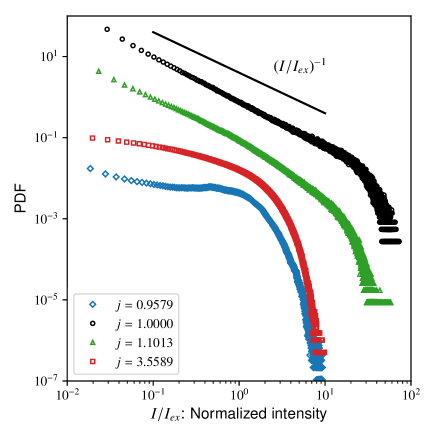
Figure 2: Probability density function (PDF) of the normalized intensity $I/I_{ex}$ obtained from the numerical simulations, where the PDFs are shifted arbitrarily in the vertical direction for visibility. The distribution of the probability density of $j=1$ (black circles) clearly exhibits an algebraic decay with exponent $\beta\simeq 1$, where the solid straight line represents $(I/I_{ex})^{-1}$. The cutoff of the distributions is maximized at $j=1$.

To demonstrate the existence of SOC-like behaviors in the laser oscillations, we here present statistical distributions of the laser intensity and intervals of the bursts calculated from the time series of the numerical simulations.

The probability density functions (PDFs) of the normalized intensity $I/I_{ex}$ are shown in Fig. 2, where the probability distributions are depicted in a double logarithmic display. Under the threshold condition ($j=1$), the distribution evidently forms a straight shape (open black circles), i.e., the distribution contains a power-law decay described by Eq. (1), over at least three orders of magnitude, where the characteristic exponent is almost unity ($\beta\simeq 1$). The exponent is close to that observed in seismic statistics known as Gutenberg–Richter’s law Gutenberg and Richter (1956). When $j>1$, the power-law decay (scale-invariant feature) disappears rapidly and transforms to an exponential one, which has a characteristic scale. When $j<1$, the power-law feature also disappears, as can be seen from the distribution represented by blue diamonds in Fig. 2. It should be noted that the cutoff intensity of the distributions, i.e., the upper bound of the event size, takes on a maximum value under the threshold condition $j=1$. We will investigate this trend in detail in Subsec. II.5.

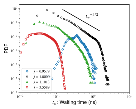
Figure 3: PDF of waiting time, the interval between successive peaks of intensity bursts, obtained with an injection current $j$. The power-law regime appears when $j=1$ (black circles), where the solid line represents a power-law curve with $\beta=1.5$.

It is known that SOC yields power-law statistics in terms of size and the time of energy-release events Bak et al. (1987); Jensen (1998); Aschwanden (2011). Here, the distributions of waiting time, i.e., the time interval between two sequential peaks of intensity bursts, are shown in Fig. 3, where we consider each burst of intensity as an energy-release event. The waiting time distribution obtained for a large pump current ($j=3.5589$) forms a convex shape around $t_{w}=$0.04\text{\,}\mathrm{n}\mathrm{s}$$. This means the existence of a characteristic time-scale of the burst events. With decreasing the pump current from the large value, a straight “shoulder,” which is an indication of a power-law character, develops in the distributions. Under the threshold condition ($j=1$), a power-law decay with $\beta\simeq 3/2$ clearly appears over approximately two orders of magnitude as depicted by open black circles in Fig. 3. This power-law feature in the waiting time is compatible with the aftershock statistics of earthquakes known as Utsu–Omori’s law, while the exponent of $3/2$ is slightly higher than that of the law Omori (1894); Utsu (1969). Similar to the case with the intensity statistics shown in Fig. 2, the power-law behavior disappears again for lower pump currents ($j<1$), which are depicted by blue diamonds in Fig. 3.

The above simulation results show that the statistical distributions of size and interval of energy-release events form power-law decays just on the threshold condition $j=1$. This indicates that semiconductor lasers with optical feedback exhibit the power-law statistics (as typically observed in SOC) in the threshold condition of the solitary mode.

II.4 Trajectory

In this subsection, we observe the intensity dynamics exhibiting power-law fluctuations as a trajectory in the phase space of time-delayed dynamical systems. For the Lang–Kobayashi model, a phase space consisting of dynamical variables, phase difference $\Phi(t)=\phi(t-\tau)-\phi(t)$ and carrier density $N(t)$, is generally employed to observe the dynamics, e.g., LFFs and RPPs Fischer et al. (1996); Heil et al. (2001); Uchida (2012). However, we here observe the phase space consisting of the laser intensity $I(t)/I_{ex}$ rather than $N(t)$ because we have focused on the large intensity fluctuation in this study.

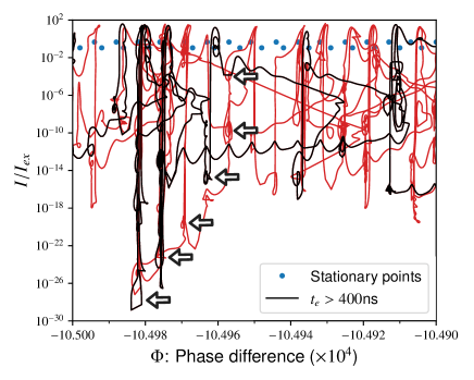
Figure 4: Part of a trajectory in the phase space constructed by phase difference $\Phi$ and normalized intensity $I/I_{ex}$ in the condition that $\tau=$1\text{\,}\mu\mathrm{s}$$, $\kappa=$60\text{\,}\mathrm{n}\mathrm{s}^{-1}$$, and $j=1$, where the solid blue circles are stationary solutions of the Lang–Kobayashi equation. The red and black curves are the trajectories in $t>$1999.5\text{\,}\mu\mathrm{s}$$ and $t>$1999.9\text{\,}\mu\mathrm{s}$$, respectively. The white arrows indicate typical pseudo stationary points (see text).

A part of a trajectory calculated from the numerical result accompanying the power-law behavior is shown in Fig. 4. Here, the simulation condition is identical to that used in Figs. 1(b) and  2: $\tau=$1\text{\,}\mu\mathrm{s}$$, $\kappa=$60\text{\,}\mathrm{n}\mathrm{s}^{-1}$$, and $j=1$. The red and black curves depicted in the figure are the trajectories after $1999.5\text{\,}\mu\mathrm{s}$ and $1999.9\text{\,}\mu\mathrm{s}$, respectively. The blue circles are the stationary points of external cavity modes. The figure shows certain unusual motions of the trajectory: the trajectory moves largely omitting many stationary points when $\Phi(t)$ decreases and increases abruptly in the direction of increasing $\Phi(t)$ (occasionally with a jerking motion). A more significant feature is a remarkable sticky motion: the trajectory is trapped around several points in the phase space where there are no stationary points. Such “pseudo” stationary points seem to be (logarithmically) homogeneously distributed in a region that extends from extremely small to large intensities in the phase space, where some of the pseudo stationary points are indicated by arrows in Fig 4. Thus, the power-law fluctuation is expected to extend to a significantly smaller region of intensity than that depicted in Fig. 2. The appearance of such multi-scale pseudo stationary points may be related to the power-law behavior in the intensity dynamics. A more detailed analysis of the phase space dynamics would be reported elsewhere.

II.5 Condition for power-law behavior

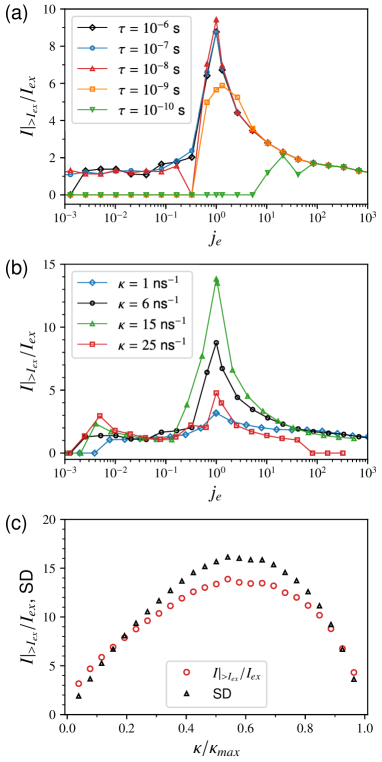
Figure 5: Mean exceedance of the intensity, $\left<I\right>|_{>I_{ex}}$, as a function of the normalized pump current $j_{e}$ or feedback strength $\kappa/\kappa_{max}$, where $\left<I\right>|_{>I_{ex}}$ is normalized by $I_{ex}$. The mean values are obtained under the condition of (a) various delay times $\tau$ and a common feedback strength $\kappa=$60\text{\,}\mathrm{n}\mathrm{s}^{-1}$$, (b) different $\kappa$ and a common delay time $\tau=$1\text{\,}\mu\mathrm{s}$$, or (c) $\tau=$1\text{\,}\mu\mathrm{s}$$ and $j_{e}=1$, where the black triangles represent the standard deviation of $\left<I\right>|_{>I_{ex}}/I_{ex}$.

In this subsection, evaluating the extent of the power-law behaviors systematically in various conditions of delay time $\tau$ and feedback strength $\kappa$, we reveal the condition of the emergence of the power-law behaviors illustrated in the previous subsection. To achieve this, we calculate the mean value of the exceedance of intensity, $\left<I\right>|_{>a}$, i.e., the size of the events beyond a reference value $a$ Sornette (2006), from the simulation results. As shown in Fig. 2, the distribution exhibits an evident power-law decay as the cutoff of the distribution increases toward the rightmost part of the figure. Thus, the mean exceedance normalized by the maximum gain mode intensity, $\left<I\right>|_{>I_{ex}}/I_{ex}$, can be a good indicator of the manifestation of power-law behaviors Sornette (2006), where we use $I_{ex}$ as the reference value for the exceedance calculation. To represent the dependence of the pump current, we employ another normalized pump current defined by

$$j_{e}\equiv\frac{J-J_{ex}}{J_{th}-J_{ex}}=\left(j-1\right)\frac{N_{th}G_{N}}{2\kappa}+1,$$ (6)

where $J_{ex}$ is the threshold pump current of the maximum gain mode defined by $J_{ex}=J_{th}\left[1-{2\kappa}/(N_{th}G_{N})\right]$ (see Appendix A). Thus, $j_{e}=0$ and $j_{e}=1$ correspond to the threshold currents of the maximum gain mode and solitary mode, respectively.

The dependence of the normalized mean exceedance $\left<I\right>|_{>I_{ex}}/I_{ex}$ on the delay time $\tau$ is shown as a function of the pump current in Fig. 5(a). Here, we employed the time series after $t=$1900\text{\,}\mu\mathrm{s}$$ to calculate the mean exceedance. The figure shows a remarkable feature that $\left<I\right>|_{>I_{ex}}/I_{ex}$ forms a sharp peak around the threshold current of the solitary mode, $j_{e}=1$, when the delay time is sufficiently long ($\tau>$1\text{\,}\mathrm{n}\mathrm{s}$$). This peak clearly represents the manifestation of the power-law behavior at the threshold of the solitary mode. The exceedance $\left<I\right>|_{>I_{ex}}/I_{ex}$ approaches unity as $j_{e}$ increases from the threshold current. This indicates that the excess pump current changes the power-law behavior accompanying extreme intensity bursts to steady oscillation with relatively small fluctuations. On the other hand, $\left<I\right>|_{>I_{ex}}/I_{ex}$ monotonically decreases as $j_{e}\to 0$ despite the divergence of $1/I_{ex}$ at $j_{e}=0$. This intensity disappearance implies that the maximum gain mode no longer works at the threshold condition of the mode.

As shown in Fig. 5(b), similar peaks indicating the emergence of the power-law behavior and the decay trend can be observed around $j_{e}=1$, but it is noteworthy that the peak disappears under an excessively large (or small) feedback strength condition. This result implies the presence of a suitable feedback strength for the power-law behavior. To identify the suitable condition, we depict the relationship between $\left<I\right>|_{>I_{ex}}/I_{ex}$ with $j_{e}=1$ and the normalized feedback strength $\kappa/\kappa_{max}$ in Fig. 5(c), where $\kappa_{max}=1/(2\tau_{p})\simeq$260\text{\,}\mathrm{n}\mathrm{s}^{-1}$$ which is the maximum value of the feedback strength as long as $I_{ex}$ is finite [see Eqs. (5) and (11)]. In the figure, the standard deviation depicted by open black triangles as well as $\left<I\right>|_{>I_{ex}}/I_{ex}$ has a maximum value at $\kappa/\kappa_{max}\simeq 0.6$.

The results presented in this subsection reveal an emergence condition of the power-law feature: the SOC-like laser oscillation with the power-law statistics emerges under the condition that the pump current is just on the threshold value of the solitary mode and the delay time is sufficiently long ($\tau>$1\text{\,}\mathrm{n}\mathrm{s}$$). In addition, the power-law behavior is most remarkable when the feedback strength is approximately 60 % of the upper limit.

III Experimental Observation

In the previous section, we have demonstrated the power-law behavior of laser intensity in the vicinity of the solitary mode with long time delay and strong feedback by performing numerical simulations. Here, we report the experimental results that support the power-law behavior of the burst intensity dynamics presented in the previous section.

III.1 Experimental setup

Figure 6 shows the experimental setup to measure the intensity time series of a semiconductor laser with delayed feedback. We used a distributed feedback (DFB) laser (operating at $1550\text{\,}\mathrm{n}\mathrm{m}$) with a fiber feedback loop. The laser light is split into two portions by a 50/50 fiber coupler. One is sent to the photodetector (Bandwidth $12\text{\,}\mathrm{G}\mathrm{H}\mathrm{z}$) via an optical isolator, and the intensity signal is measured with a digital oscilloscope (Bandwidth $16\text{\,}\mathrm{G}\mathrm{H}\mathrm{z}$, 100 GSamples/s). The other is sent to an optical fiber amplifier and fed back to the DFB laser again. In this experiment, the laser current was fixed at $12.04\text{\,}\mathrm{m}\mathrm{A}$ ($\sim 1.2$ times of the threshold current) to measure the laser intensity signal clearly. The delay time was set as approximately $116\text{\,}\mathrm{n}\mathrm{s}$, which is sufficiently long to induce the power-law like behavior. We used the optical fiber amplifier to achieve a strong optical feedback, and controlled the feedback ratio (represented by $R$) between the feedback power and output power from the laser to be within the range from $0\text{\,}\%$ to $22\text{\,}\%$.

It should be noted that the power-law behavior is difficult to measure in the present experiment because of the limitation of the dynamic range of the measurement, i.e., the limitation of the measurement range of the 8 bit analog-digital converter in the oscilloscope. Thus, the present experiment focus on the appearance of the intermittent burst of the intensity pulses, which is a signature of the power-law behavior reported in the previous section.

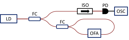
Figure 6: Experimental setup for a semiconductor laser with delayed feedback. LD, distributed feedback (DFB) laser diode; FC, 50/50 fiber coupler; ISO, optical isolator; PD, photodetector; OSC, oscilloscope; OFA, optical fiber amplifier. The fiber loop is composed of polarization-maintaining fibers.

III.2 Temporal behavior

Fig. 7 shows typical examples of intensity time series of laser oscillation obtained from our experiments at $J=$12.04\text{\,}\mathrm{m}\mathrm{A}$$. The time series at a low feedback-power ratio of $R=$6.6\text{\,}\%$$ does not indicate a significant burst [Fig. 7(a)]. On the other hand, irregular intensity bursts emerge when $R$ increases [Fig. 7(b)] and become inactive for a large feedback ratio of $R=$22.5\text{\,}\%$$, where the intensity fluctuates around a mean value. This dependence on feedback strength is consistent with our simulation results depicted in Figs 5(b) and (c).

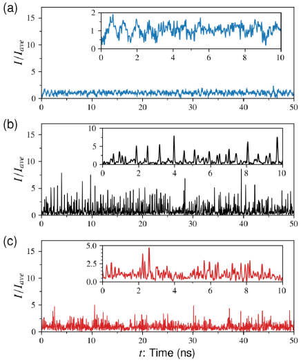
Figure 7: Time series of light intensity at (a) $R=6.6\%$, (b) $13\%$ and (c) $22.5\%$. Enlarged time series are presented in each figure.

III.3 Statistical distribution

Probability density functions of the intensity obtained from the experimental time series at certain typical conditions are shown in Fig. 8(a), where the time series until $40\text{\,}\mu\mathrm{s}$ is used for the calculation. In the figure, the distributions are shifted arbitrarily in the vertical direction for visibility.

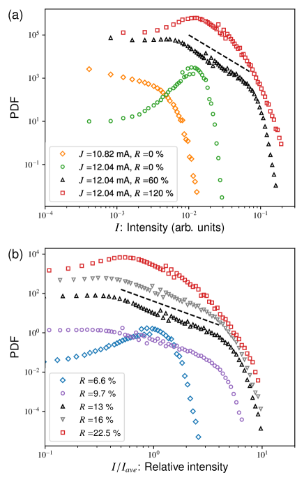
Figure 8: Experimentally obtained PDF of intensity. Here, all the plots are shifted arbitrarily in the vertical direction for visibility. (a) Intensity distributions obtained under the condition. The distribution of $J=$10.82\text{\,}\mathrm{m}\mathrm{A}$$ and $R=$0\text{\,}\%$$ is shown by orange diamonds, where the laser oscillates did not occur. The others are the distributions with $J=$12.04\text{\,}\mathrm{m}\mathrm{A}$$ and different feedback strengths $R$. (b) Intensity distribution normalized by the mean intensity $I_{ave}$. All the pump currents are set as $J=$12.04\text{\,}\mathrm{m}\mathrm{A}$$. The dashed lines represent the power-law curve with the exponent $\beta=2$.

A sufficient pump current for laser oscillation without delayed feedback ($J=$12.04\text{\,}\mathrm{m}\mathrm{A}$$, $R=$0\text{\,}\%$$) yields only a Gaussian-like distribution, which is depicted as green circles in the figure. This reflects the fluctuation behavior near the mean intensity. When the optical feedback is applied, the fluctuation is increased dramatically, and the regime of power-law-like decay appears in the statistical distribution. As shown by the black triangles in Fig. 8(a), the power-law regime is indicated by the dashed line in the figure, and the characteristic exponent is approximately two ($\beta\simeq 2$). This experimental condition ($J=$12.04\text{\,}\mathrm{m}\mathrm{A}$$, $R=$13\text{\,}\%$$) is identical to that of Fig. 7(b).

As our numerical simulations predict that this power-law behavior disappears when the feedback strength is significantly larger, the same tendency can be observed in the present experiments. Fig. 8(b) shows statistical distributions of relative intensity under the fixed pump current ($J=$12.04\text{\,}\mathrm{m}\mathrm{A}$$) and different feedback strengths ($R=6.6,9.7,13$, and $22.5\text{\,}\%$), where the intensity is normalized by the mean intensity $I_{\text{ave}}$. The figure reveals that the power-law regime becomes prominent in the distribution when the feedback strength increases, but becomes less prominent when the strength exceeds $13\text{\,}\%$. The cutoff of the distributions, i.e., the maximum relative intensity, also has a character similar to that of the numerical results as shown in Fig. 2: the cutoff becomes maximum at $R=$13\text{\,}\%$$ even the difference among the cutoffs is also not clear.

IV Discussion

This study shows that intermittent intensity bursts characterized by power-law statistics emerge and are prominent when the delayed feedback is sufficiently long and strong and the pump current is just on the lasing threshold. The reason why the power-law fluctuation is remarkable in this situation can be explained from the perspective of the emergence condition of SOC as mentioned in Section I. SOC can emerge in a specific dissipative system that has (i) multiple energy release processes with (ii) thresholds, (iii) mutual interaction and (iv) energy injection that is sufficiently slower than the release processes.

The external energy injection of the laser system considered in this study is the pump current $j$. In laser systems without feedback, the slowest driving rate corresponds to the threshold current ($j=1$) rather than zero pump current ($j=0$). This is because the carrier density of the laser decays with lifetime $\tau_{s}$ even in the absence of energy release by laser oscillation [see Eq. (3)]. Thus, the threshold current can be regarded as the ideal situation that satisfies the fourth condition. The number of virtual nodes of a time-delay dynamical system is proportional to the delay time $\tau$ Uchida (2012). Furthermore, the strength of the interaction between the feedback and laser intensity is determined by the coupling strength of the feedback, $\kappa$. Hence, a sufficiently long $\tau$ is required for the multiplicity (high dimensionality) of the energy release process, and a strong $\kappa$ firmly establishes their interactions. Therefore, it is reasonable that the power-law fluctuation is prominent in the situation. However, certain results cannot be explained directly by the occurrence conditions of SOC. As shown in Figs. 5(a) and (b), the power-law behavior is prominent when $j_{e}=1$ rather than when $j_{e}=0$. It is a wonder that the onset of the power-law behavior is determined by the threshold of the solitary mode $j_{e}=1$ rather than that of the external cavity modes $j_{e}=0$, although the power-law behaviors depend strongly on the external feedback light. In future works, more efforts should be undertaken to explain the optimum value of the feedback strength, $\kappa/\kappa_{max}\simeq 0.6$, to obtain remarkable power-law fluctuations as shown in Fig. 5(c).

Next, we mention the discordance between the experimental and numerical results. The width of the power-law regime and the characteristic exponent obtained in our experiments vary slightly from the simulation results. The power-law regime obtained in the experiments is limited to one order of magnitude [from $I=0.01$ to $0.1$ in Fig. 8(a)] unlike the numerical results (Fig. 2). The lower bound would result from the noise of the measurement, whose size can be measured as the distribution in the non-oscillatory condition depicted by orange diamonds in Fig. 8(a). This noise region is almost consistent with the lower bound of the power-law regime of the experiments. The dynamic range of the measurement equipment used in the experiments is also a reason for the lower bound. The large characteristic exponent $\beta\simeq 2$ in the experiment compared with that in the simulations may have originated from the gain saturation of the laser and incomplete tuning of the pump current to the threshold value. The saturation effect reduces the cutoff of the intensity distributions (see Appendix B). The combination of the saturation effect and the excess pump current due to the incomplete tuning causes a partial increase in the gradient of the intensity distribution to $1.8$ (Fig. 9).

Here, we indicate that the burst behavior is different from previously reported dynamical behaviors such as chaotic oscillations, RPPs, and LFFs. The pulses that construct the bursts may appear to be similar to RPPs, but, unlike RPPs, periodicity of the pulses is absent Heil et al. (2001); Uchida (2012). Even though the regular dropouts peculiar to LFFs are not observed in the burst behavior Fischer et al. (1996); Heil et al. (1998); Ohtsubo (2012); Uchida (2012), LFFs may be associated with the power-law behaviors. This is because the condition for the emergence of the power-law bursts is close to that for LFFs except for the delay time. According to our investigation, depending on the feedback strength, regular drops can be observed when $\tau_{D}\lesssim$0.05\text{\,}\mathrm{n}\mathrm{s}$$, and a longer delay time causes the time series to be irregular. Future studies would elucidate the connection between the present power-law bursts and LFFs.

Nonequilibrium critical phenomena, namely SOC mentioned here, are closely related to nonequilibrium phase transitions, particularly the absorbing-state phase transition Muñoz et al. (1999); Vespignani et al. (2000); Henkel et al. (2008). In fact, absorbing-state phase transition has been observed in a semiconductor laser with delayed feedback similar to that in the present study Faggian et al. (2018). It is also noteworthy that the dynamical systems with time delays can produce SOC-like behaviors, in contrast to the fact that the conventional models that reproduce SOC and absorbing-state phase transitions generally consist of cellular automata Bak et al. (1987, 1988); Jensen (1998); Aschwanden (2011). The manner in which the delay system produces the power-law behaviors can be observed as a trajectory in the phase space as depicted in Fig. 4. Since most of the discussion on the relationship between the present results and SOC is conjectural, the detailed mechanism that produces the SOC features in delay systems should be elucidated in future studies. It might enable the understanding of nonequilibrium critical phenomena and phase transitions from the aspect of dynamical systems in the presence of delayed feedback.

V Conclusion

In the present simulations and experiments, we demonstrated that the semiconductor lasers with a sufficiently strong and long delayed feedback at the critical point (lasing threshold) can cause the intermittent intensity fluctuation characterized by power-law distributions peculiar to nonequilibrium critical phenomena, specifically self-organized criticality (SOC). The results of the numerical simulations of the Lang–Kobayashi model show that the laser intensity exhibits irregular bursts consisting of spike-like pulsation. As a result, certain peak values of the bursts attain several tens of times the intensity of the maximum gain mode. This is quantitatively different from other currently reported behaviors such as low-frequency fluctuations, regular pulse packages, or chaotic oscillations. Similar behaviors were experimentally measured in a semiconductor laser with delayed feedback. The intensity bursts are most remarkable when the coupling of the feedback is moderately strong ($60\%$ of the maximum feedback strength), the delay time is sufficiently long ($\tau>$1\text{\,}\mathrm{n}\mathrm{s}$$), and the pump current is just on the threshold value of the solitary mode. The noteworthy feature is that the intensity and waiting time of the bursts follow power-law distributions with exponents of approximately $1$ and $2/3$, respectively. This statistical feature can be interpreted as a signature of SOC.

Appendix A Characteristic values of external cavity modes

To investigate the intensity dynamics of the lasers, in this research, we employed certain quantities that represent external cavity modes of semiconductor lasers described by the Lang–Kobayashi equations; the oscillation intensity of maximum gain mode $I_{ex}$, threshold current of the external cavity modes $J_{ex}$, and maximum strength of the delayed feedback $\kappa_{max}$. Although these are described in commonly available textbooks Uchida (2012), we introduce these quantities in this appendix for the reader’s convenience.

The intensity generated from the maximum gain mode can be estimated by considering the stationary state of the Lang–Kobayashi equation: ${\text{d}\hat{E}}/{\text{d}t}{}={\text{d}N}/{\text{d}t}{}=0$. The stationary carrier density $N_{s}$ when ${\text{d}\hat{E}}/{\text{d}t}{}=0$ is obtained from Eq. (2):

$$N_{s}=N_{th}-\frac{2\kappa}{G_{N}}\cos\omega_{s}\tau$$ (7)

where $N_{th}=N_{0}+{1}/({\tau_{p}G_{0}})$, and $\omega_{s}$ is a stationary angular frequency. Substituting the carrier density into Eq. (3), we can obtain the stationary intensity of external cavity modes described by the square of $\hat{E}$:

$$I_{s}=\frac{\tau_{p}}{G_{N}\tau_{s}}\frac{(j-1)N_{th}G_{N}+2\kappa\cos\omega_{s}\tau}{1-2\tau_{p}\kappa\cos\omega_{s}\tau},$$ (8)

where $j$ is the normalized pump current defined by $j=J/J_{th}$, and $J_{th}=N_{th}/\tau_{s}$. Because $I_{s}$ is determined by the angular frequency of a mode $\omega_{s}$, it is maximized when $\cos\omega_{s}\tau=1$. Hence, the intensity of the maximum gain mode that we used to normalize the intensity of oscillation in this study can be represented by

$$I_{ex}=\frac{1}{G_{N}}\frac{\tau_{p}}{\tau_{s}}\frac{(j-1)N_{th}G_{N}+2\kappa}{1-2\tau_{p}\kappa}.$$ (9)

The condition $I_{ex}=0$ means that at least one external cavity mode begins to oscillate. Thus, the external cavity mode can activate at the normalized pump current $j=1-{2\kappa}/({N_{th}G_{N}})$. Then the threshold pump current is represented by

$$J_{ex}=J_{th}\left(1-\frac{2\kappa}{N_{th}G_{N}}\right).$$ (10)

From the denominator of Eq. (9), we can recognize that the stationary intensity is finite unless $2\tau_{p}\kappa\geq 1$. Therefore, the maximum feedback strength that we can set is determined by

$$\kappa_{max}=(2\tau_{p})^{-1}.$$ (11)

These estimations are good approximations as long as the number of external cavity modes is sufficiently large.

Appendix B Saturation effect of gain

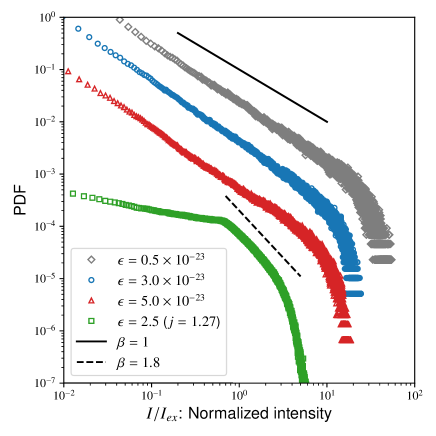
Figure 9: PDF of oscillation intensity for different gain saturation parameters $\epsilon$ with the threshold injection current $j=1$, where the distribution depicted by green squares is for $\epsilon=$2.5\text{\times}{10}^{-23}\text{\,}\mathrm{m}^{3}$$ and $j=1.2652$. For visibility, power-law curves with exponents $\beta=1$ and $1.8$ are shown by solid and dashed lines, respectively.

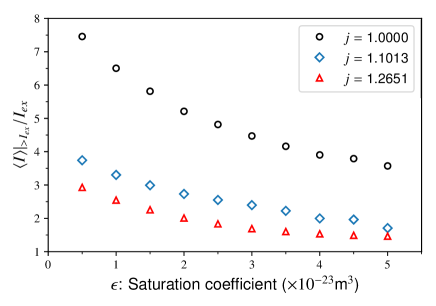
Figure 10: The mean exceedance of the intensity for different injection currents $j$ as a function of the saturation parameter $\epsilon$, where the exceedance is normalized by $I_{ex}$.

To extract the essence of power-law behaviors in semiconductor lasers with delayed feedback, we omitted the effect of gain saturation of the laser in the simulations of this study. However, the saturation effect is essential for comparing the present simulations with the experiments. Here, we show the influence of the gain saturation upon the intensity distributions by performing simulations of the Lang–Kobayashi model with the nonvanishing gain saturation parameter $\epsilon$ shown in Eq. (4). For the simulations, we applied some values of the saturation parameter in the range from $\epsilon=$0.1\text{\times}{10}^{-23}\text{\,}\mathrm{m}^{3}$$ to $5.0\text{\times}{10}^{-23}\text{\,}\mathrm{m}^{3}$, where the range includes the value of actual lasers used in ordinary experiments Harayama et al. (2011); Mikami et al. (2012).

The intensity distributions with three gain saturation parameters are shown in Fig. 9, where the gray diamonds, blue circles, and red triangles correspond to $\epsilon=$0.5\text{\times}{10}^{-23}\text{\,}$$, $3.0\text{\times}{10}^{-23}\text{\,}$, and $0.5\text{\times}{10}^{-23}\text{\,}\mathrm{m}^{3}$, respectively, and the pump current of the three distribution is set as the threshold value of the solitary mode ($j=1$). As is evident from the figure, the results of $\epsilon=$0.5\text{\times}{10}^{-23}\text{\,}$$ and $3.0\text{\times}{10}^{-23}\text{\,}\mathrm{m}^{3}$ exhibit power-law distributions with $\beta\simeq 1$ that are identical to those obtained by the simulations with $\epsilon=0$. The larger saturation parameter ($\epsilon=$5.0\text{\times}{10}^{-23}\text{\,}\mathrm{m}^{3}$$) affects its distribution slightly.

A more significant influence of the gain saturation is a decrease in the cutoff of the distributions with an increase in $\epsilon$. This trend can be confirmed more clearly in Fig. 10, where the mean exceedance above $I_{ex}$ is plotted as a function of $\epsilon$. The figure indicates that the maximum intensity caused by oscillation bursts decreases monotonically with $\epsilon$ regardless of $j$. Another notable result can be observed in the distribution as shown by green squares in Fig. 9. Here, its saturation parameter, $\epsilon=$2.5\text{\times}{10}^{-23}\text{\,}\mathrm{m}^{3}$$, is comparable with that used for the present experiments described in Sec. III, and the pump current is slightly larger than the solitary mode threshold, $j=1.2652$. The distribution indicates that a synergy between the gain saturation and the excess of the current disrupts a wide range of power-law regimes, and the gradient of the power-law regime of the distribution increases more than $\beta=1.8$. This implies that power-law statistics different from that obtained in the simulations can be observed in the experimental measurements because it is hard to tune the injection current just to the threshold value of the solitary mode and the saturation effect is consistently present in actual lasers.

References

- DeGiorgio and Scully (1970) V. DeGiorgio and M. O. Scully, Analogy between the laser threshold region and a second-order phase transition, Phys. Rev. A 2, 1170 (1970).
- Graham and Haken (1970) R. Graham and H. Haken, Laserlight —first example of a second-order phase transition far away from thermal equilibrium, Zeitschrift für Physik 237, 31 (1970).
- Rice and Carmichael (1994) P. R. Rice and H. J. Carmichael, Photon statistics of a cavity-qed laser: A comment on the laser–phase-transition analogy, Phys. Rev. A 50, 4318 (1994).
- Kuo et al. (2012) W.-C. Kuo, Y.-H. Wu, Y.-C. Li, and T.-C. Yen, Criticalities and phase transitions in the polarization switching of vertical-cavity surface-emitting lasers, IEEE Photonics Technology Letters 24, 2262 (2012).
- Basak et al. (2016) S. Basak, A. Blanco, and C. López, Large fluctuations at the lasing threshold of solid- and liquid-state dye lasers, Scientific Reports 6, 32134 (2016).
- Wang et al. (2017) T. Wang, H. Vergnet, G. P. Puccioni, and G. L. Lippi, Dynamics at threshold in mesoscale lasers, Phys. Rev. A 96, 013803 (2017).
- Wang et al. (2020) T. Wang, G. P. Puccioni, and G. L. Lippi, Photon bursts at lasing onset and modelling issues in micro-vcsels, Journal of Modern Optics 67, 55 (2020).
- Bak et al. (1987) P. Bak, C. Tang, and K. Wiesenfeld, Self-organized criticality: An explanation of the 1/ f noise, Phys. Rev. Lett. 59, 381 (1987).
- Bak et al. (1988) P. Bak, C. Tang, and K. Wiesenfeld, Self-organized criticality, Phys. Rev. A 38, 364 (1988).
- Jensen (1998) H. J. Jensen, Self-Organized Criticality: Emergent Complex Behavior in Physical and Biological Systems (Cambridge Lecture Notes in Physics) (Cambridge University Press, 1998).
- Sornette (2006) D. Sornette, Critical phenomena in natural sciences: chaos, fractals, selforganization and disorder: concepts and tools (Springer Science & Business Media, 2006).
- Aschwanden (2011) M. Aschwanden, Self-organized criticality in astrophysics: The statistics of nonlinear processes in the universe (Springer, 2011).
- Omori (1894) F. Omori, On the after-shocks of earthquakes, J. Coll. Sci., Imp. Univ., Japan 7, 111 (1894).
- Utsu (1969) T. Utsu, Aftershocks and earthquake statistics (i) : Some parameters which characterize an aftershock sequence and their interrelations, J. Faculty Sci., Hokkaido University, Ser. VII (Geophys.) 3, 129 (1969).
- Miguel et al. (2001) M. C. Miguel, A. Vespignani, S. Zapperi, J. Weiss, and J.-R. Grasso, Intermittent dislocation flow in viscoplastic deformation, Nature 410, 667 (2001).
- Niiyama and Shimokawa (2015) T. Niiyama and T. Shimokawa, Atomistic mechanisms of intermittent plasticity in metals: Dislocation avalanches and defect cluster pinning, Phys. Rev. E 91, 022401 (2015).
- Durin and Zapperi (2000) G. Durin and S. Zapperi, Scaling exponents for barkhausen avalanches in polycrystalline and amorphous ferromagnets, Phys. Rev. Lett. 84, 4705 (2000).
- Field et al. (1995) S. Field, J. Witt, F. Nori, and X. Ling, Superconducting vortex avalanches, Phys. Rev. Lett. 74, 1206 (1995).
- Ikeda and Matsumoto (1987) K. Ikeda and K. Matsumoto, High-dimensional chaotic behavior in systems with time-delayed feedback, Physica D: Nonlinear Phenomena 29, 223 (1987).
- Arecchi et al. (1992) F. T. Arecchi, G. Giacomelli, A. Lapucci, and R. Meucci, Two-dimensional representation of a delayed dynamical system, Phys. Rev. A 45, R4225 (1992).
- Giacomelli and Politi (1996) G. Giacomelli and A. Politi, Relationship between delayed and spatially extended dynamical systems, Phys. Rev. Lett. 76, 2686 (1996).
- Uchida (2012) A. Uchida, Optical communication with chaotic lasers: applications of nonlinear dynamics and synchronization (John Wiley & Sons, 2012).
- Erneux et al. (2017) T. Erneux, J. Javaloyes, M. Wolfrum, and S. Yanchuk, Introduction to focus issue: Time-delay dynamics, Chaos: An Interdisciplinary Journal of Nonlinear Science 27, 114201 (2017).
- Ohtsubo (2012) J. Ohtsubo, Semiconductor lasers: stability, instability and chaos, vol. 111 (Springer, 2012).
- Heil et al. (2001) T. Heil, I. Fischer, W. Elsäßer, and A. Gavrielides, Dynamics of semiconductor lasers subject to delayed optical feedback: The short cavity regime, Phys. Rev. Lett. 87, 243901 (2001).
- Ikeda et al. (1980) K. Ikeda, H. Daido, and O. Akimoto, Optical turbulence: Chaotic behavior of transmitted light from a ring cavity, Phys. Rev. Lett. 45, 709 (1980).
- Fischer et al. (1996) I. Fischer, G. H. M. van Tartwijk, A. M. Levine, W. Elsässer, E. Göbel, and D. Lenstra, Fast pulsing and chaotic itinerancy with a drift in the coherence collapse of semiconductor lasers, Phys. Rev. Lett. 76, 220 (1996).
- Heil et al. (1998) T. Heil, I. Fischer, and W. Elsäßer, Coexistence of low-frequency fluctuations and stable emission on a single high-gain mode in semiconductor lasers with external optical feedback, Phys. Rev. A 58, R2672 (1998).
- Reinoso et al. (2013) J. A. Reinoso, J. Zamora-Munt, and C. Masoller, Extreme intensity pulses in a semiconductor laser with a short external cavity, Phys. Rev. E 87, 062913 (2013).
- Bosco et al. (2013) A. K. D. Bosco, D. Wolfersberger, and M. Sciamanna, Extreme events in time-delayed nonlinear optics, Opt. Lett. 38, 703 (2013).
- Choi et al. (2016) D. Choi, M. J. Wishon, J. Barnoud, C. Y. Chang, Y. Bouazizi, A. Locquet, and D. S. Citrin, Low-frequency fluctuations in an external-cavity laser leading to extreme events, Phys. Rev. E 93, 042216 (2016).
- Bosco et al. (2017) A. K. D. Bosco, N. Sato, Y. Terashima, S. Ohara, A. Uchida, T. Harayama, and M. Inubushi, Random number generation from intermittent optical chaos, IEEE Journal of Selected Topics in Quantum Electronics 23, 1 (2017).
- Barbosa et al. (2019) W. A. S. Barbosa, E. J. Rosero, J. R. Tredicce, and J. R. Rios Leite, Statistics of chaos in a bursting laser, Phys. Rev. A 99, 053828 (2019).
- Appeltant et al. (2011) L. Appeltant, M. C. Soriano, G. Van der Sande, J. Danckaert, S. Massar, J. Dambre, B. Schrauwen, C. R. Mirasso, and I. Fischer, Information processing using a single dynamical node as complex system, Nature Communications 2, 468 (2011).
- Larger et al. (2017) L. Larger, A. Baylón-Fuentes, R. Martinenghi, V. S. Udaltsov, Y. K. Chembo, and M. Jacquot, High-speed photonic reservoir computing using a time-delay-based architecture: Million words per second classification, Phys. Rev. X 7, 011015 (2017).
- Lang and Kobayashi (1980) R. Lang and K. Kobayashi, External optical feedback effects on semiconductor injection laser properties, IEEE Journal of Quantum Electronics 16, 347 (1980).
- Gutenberg and Richter (1956) B. Gutenberg and C. F. Richter, Earthquake magnitude, intensity, energy, and acceleration, Bulletin of the Seismological Society of America 46, 105 (1956).
- Muñoz et al. (1999) M. A. Muñoz, R. Dickman, A. Vespignani, and S. Zapperi, Avalanche and spreading exponents in systems with absorbing states, Phys. Rev. E 59, 6175 (1999).
- Vespignani et al. (2000) A. Vespignani, R. Dickman, M. A. Muñoz, and S. Zapperi, Absorbing-state phase transitions in fixed-energy sandpiles, Phys. Rev. E 62, 4564 (2000).
- Henkel et al. (2008) M. Henkel, H. Hinrichsen, and S. Lübeck, Non-equilibrium phase transitions: volume 1: absorbing phase transitions (Springer Science & Business Media, 2008).
- Faggian et al. (2018) M. Faggian, F. Ginelli, F. Marino, and G. Giacomelli, Evidence of a critical phase transition in purely temporal dynamics with long-delayed feedback, Phys. Rev. Lett. 120, 173901 (2018).
- Harayama et al. (2011) T. Harayama, S. Sunada, K. Yoshimura, P. Davis, K. Tsuzuki, and A. Uchida, Fast nondeterministic random-bit generation using on-chip chaos lasers, Phys. Rev. A 83, 031803 (2011).
- Mikami et al. (2012) T. Mikami, K. Kanno, K. Aoyama, A. Uchida, T. Ikeguchi, T. Harayama, S. Sunada, K.-i. Arai, K. Yoshimura, and P. Davis, Estimation of entropy rate in a fast physical random-bit generator using a chaotic semiconductor laser with intrinsic noise, Phys. Rev. E 85, 016211 (2012).