Predicting conductivities of alkali borophosphate glasses based on site energy distributions derived from network former unit concentrations

Abstract

For ion transport in network glasses, it is a great challenge to predict conductivities specifically based on structural properties. To this end it is necessary to gain an understanding of the energy landscape where the thermally activated hopping motion of the ions takes place. For alkali borophosphate glasses, a statistical mechanical approach was suggested to predict essential characteristics of the distribution of energies at the residence sites of the mobile alkali ions. The corresponding distribution of site energies was derived from the chemical units forming the glassy network. A hopping model based on the site energy landscape allowed to model the change of conductivity activation energies with the borate to phosphate mixing ratio. Here we refine and extend this general approach to cope with minimal local activation barriers and to calculate dc-conductivities without the need of performing extensive Monte-Carlo simulations. This calculation relies on the mapping of the many-body ion dynamics onto a network of local conductances derived from the elementary jump rates of the mobile ions. Application of the theoretical modelling to three series of alkali borophosphate glasses with the compositions $0.33$Li₂O$-0.67$[$x$B₂O₃-$(1\!-\!x)$P₂O₅], $0.35$Na₂O$-0.65$[$x$B₂O₃-$(1\!-\!x)$P₂O₅] and $0.4$Na₂O$-0.6$[$x$B₂O₃-$(1\!-\!x)$P₂O₅] shows good agreement with experimental data.

I Introduction

Solid electrolytes are used in chemical sensors Fergus (2011), electrochromic devices Yoo et al. (2006), optical wave guides Tervonen et al. (2011), supercapacitors Samui and Sivaraman (2010), and batteries Kim et al. (2015). Compared to liquid electrolytes, they have in general higher energy and power densities, and their use in all-solid-state batteries allows for a safer operation of electronic devices and electric cars. A good understanding of ion transport in solid electrolytes is needed to further optimise the chemical and physical properties of these materials for various applications.

A prerequisite for a material-specific understanding of the ion transport is a knowledge of energy landscapes that describe how the interaction energy of the mobile ions with the immobile constituents of the host matrix varies in space. In defective crystalline materials, the energy landscapes may be determined by introducing interaction parameters describing all relevant local configurations of immobile atoms/ions in the environment of the mobile ions. Corresponding interaction parameters can be determined by ab initio methods Koettgen et al. (2018) or, if small in number, by fitting to experimental results Meyer et al. (1996).

In glassy electrolytes, it poses a particular challenge to gain knowledge of the energy landscape because of the amorphous structure of these materials. For understanding generic (non-material specific) features of the ionic transport behaviour, it is justified to merely assume that some distributions of site and/or barrier energies exist Dyre et al. (2009). This has been done, for example, to understand the origin of the mixed alkali effect Maass (1999); Hunt (1999), of non-Arrhenius behaviour in fast ion conducting glasses Maass et al. (1996) and universal properties of conductivity spectra in ion conducting glasses Baranovskii and Cordes (1999); Dyre and Schrøder (2000); Porto et al. (2000); Dieterich and Maass (2002). For a material specific modelling, one could apply molecular dynamics (MD) simulations Habasaki and Hiwatari (2004); Lammert et al. (2009); Vogel (2004) but it is not clear at present whether information on the energy landscapes extracted from such simulations is reliable. This is due to questions about the quality of force fields and due to the problem that structures obtained from a cooling protocol in simulations may not reflect the ones obtained in experiments.

An attempt to derive energetically favourable diffusion paths of mobile ions in oxide glasses based on experimental observations was suggested by combining reverse Monte Carlo (RMC) modelling with a bond valence analysis Adams and Swenson (2000, 2005). In that approach, amorphous structures are obtained by RMC modelling of neutron and Xray diffraction data. Subsequently, preferred diffusion paths for the mobile ions are identified by considering chemical constraints (primarily minimal distances to network forming ions) and an upper bound for deviations of the mobile ions’ bond valence to oxygen ions from an ideal value. However, in an MD study of a lithium silicate glass Müller et al. (2007), this approach failed to identify correctly the ion sites in the glassy network, i.e. the regions where mobile ions reside for a much longer time compared to other regions. Also, concentrations of network forming units (NFUs) in mixed glass former glasses could not be correctly reproduced by the RMC modelling of diffraction data Karlsson et al. (2015); Schuch et al. (2012)

A method for constructing site energy landscapes in ion conducting network glasses was suggested in Ref. Schuch et al. (2011). It is based on the idea that the dominant contribution to the spatial variation of the energy landscape originates from the counter charges of the alkali ions. These counter charges are provided by charged NFUs that are irregularly distributed in the glassy network. The method has so far been applied to alkali borophosphate glasses, where in the theoretical modelling an uncorrelated random spatial distribution of the NFUs is assumed. Eight different types of NFU units were identified by magic-spinning nuclear magnetic resonance (MAS-NMR Silver and Bray (1958); Eckert (2018); Youngman (2018)) in these glasses and the experimentally determined concentrations of NFUs could be well explained by a statistical mechanical modelling Schuch et al. (2011); Bosi et al. (2021).

The site energy landscape constructed from the NFU concentration was in the following used as an essential input for a hopping model of the thermally activated ionic motion in the glassy network. Long-range diffusion coefficients and their activation energies resulting from this hopping model were first calculated by KMC simulations. The simulated variation of the activation energies with the borate to phosphate mixing ratio turned out to be in very good agreement with experimental observations Schuch et al. (2011).

In a recent study Bosi et al. (2021) it was shown that the activation energies can be even derived without KMC simulations by applying the theory developed in Ref. Ambegaokar et al. (1971). We find it remarkable that one can predict structural properties and a connection to ion transport quantities in these complex disordered materials by rather simple numerical calculations based on analytical theories, that means without performing extensive simulations of the network structure and ionic motion.

Here we refine and extend the analytical approach used in Ref. Bosi et al. (2021) and investigate whether not only activation energies can be successfully modelled but also dc-conductivities. To this end, we use the mapping of the many-body hopping dynamics to a network of conductances introduced in Ref. Ambegaokar et al. (1971). The conductivities are determined by solving Kirchhoff’s equations for the conductance network with the Kron reduction method Dörfler and Bullo (2013). In addition we take into account a minimal local activation energy for elementary ion jumps. The theoretical modelling is applied to three series of alkali borophosphate glasses and compared to experimental data.

II Site Energy Landscapes derived from modelling of MAS-NMR data

The network of alkali borophosphate glasses is built by various borate units B⁽ⁿ⁾ and phosphate units P^(m), where $n$ and $m$ are specifying the number of bridging oxygens (bOs). These units could be identified by MAS-NMR Zielniok et al. (2007); Rinke and Eckert (2011); Larink et al. (2012). As depicted in Fig. 1, there exists one negatively charged tetrahedral borate unit B⁽⁴⁾, and two trigonal borate units B⁽³⁾ and B⁽²⁾, where the B⁽³⁾ is neutral and the B⁽²⁾ unit has one negative charge localised mainly at its non-bridging oxygen (nbO, marked in red in Fig. 1). By contrast, the negative charge of the B⁽⁴⁾ can be considered as delocalised over all bOs. The phosphate units P^(m) all have a tetragonal conformation and a negative charge $(m-3)$ in units of the elementary charge. These charges should be mainly localised at the nbOs and can be viewed to be shared between these nbOs, i.e. between two nbOs for P⁽²⁾, three nbOs for P⁽¹⁾, and four nbOs for P⁽⁰⁾. For borophosphate glasses with low molar alkali content smaller than 30%, positively charged P⁽⁴⁾ units may occur Rinke and Eckert (2011). In this study, however, we are not considering such low alkali contents, which means that the glass networks are formed by the units shown in Fig. 1.

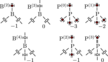
Figure 1: Sketch of the units forming the glass network in alkali borophosphate glasses for molar alkali contents larger than 30% (for lower alkali content, positively charged P⁽⁴⁾ units may appear Bosi et al. (2021)). The numbers indicate the charge of the units and the nbOs of each unit are marked in red.

The concentrations of the respective NFU units vary with both the borate to phosphate mixing ratio and the alkali content. A statistical mechanical model was developed in our group to predict these variations Schuch et al. (2011). Explicit analytical expressions are given in Ref. Bosi et al. (2021) if disregarding possible disproportionation reactions between certain units. The theoretical predictions compare very well with the ones extracted from MAS-NMR measurements. When generating site energy landscapes as described in the following, we always used the NFU concentrations predicted by the theory.

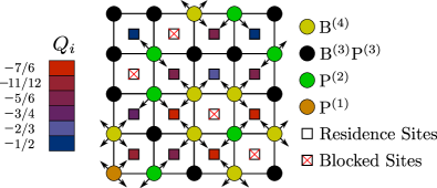
Figure 2: Illustration of the generation of the site energy landscape. The NFUs are randomly distributed among the sites of a simple cubic lattice (here square lattice) and induce charges at the centres of the lattice cells (given in units of the elementary charge). These centres are either residence sites of the mobile ions (“ion sites”) or blocked sites. At each ion site, a charge $Q_{i}$ is generated by the surrounding NFUs, which gives rise to a (non-smeared) energy $V_{0}Q_{i}$ at site $i$, see Eq. (2). Specifically, an NFU with charge $q_{\alpha}$ and $k_{\alpha}$ nbOs adds a partial contribution $-q_{\alpha}/k_{\alpha}$ to $k_{\alpha}$ randomly selected neighbouring ion sites. A P⁽²⁾ unit, for example, gives a charge contribution -1/2 to two sites. The delocalised charge -1 of a B⁽⁴⁾ unit induces an equal contribution to all its surrounding ion sites (indicated by circles). This contribution thus is $-1/z$, where $z$ is the number of non-blocked sites in the environment of the B⁽⁴⁾ unit (for the square lattice $z\leq 4$, while $z\leq 8$ in the simple cubic lattice). The partial charges induced by the NFUs are indicated by the arrows and they sum up to the total countercharge $Q_{i}$. Different levels of the $Q_{i}$ are represented by the color coding.

Knowing the NFU concentrations, site energy landscapes are created by the procedure sketched in Fig. 2 Schuch et al. (2011); Bosi et al. (2021). For simplicity, we consider one of the two interpenetrating simple cubic sublattices of a bcc lattice as the positions of the NFUs and refer to it as the NFU lattice. Each site of this NFU lattice is occupied by an NFU with a probability given by its concentration weight without taking into account spatial correlations.

The $N_{\rm tot}$ sites of the other simple cubic sublattice contain the $N_{\rm acc}$ ion sites (residence sites of the mobile ions). A fraction $f_{0}$ of these accessible sites is empty. In MD simulations, $f_{0}$ was found to be in the range of 5-10%. That $f_{0}$ must be small follows also from theoretical considerations to explain internal friction measurements Peibst et al. (2005); Maass and Peibst (2006). The $N_{\rm acc}$ sites consist of $N$ occupied ion sites ($N$: number of ions) and $N_{\rm vac}$ vacant ion sites, $N_{\rm acc}=N+N_{\rm vac}$. The remaining sites in the respective sublattice are regarded as blocked (non-accessible) for the mobile ions. Their number is $N_{\rm bl}=N_{\rm tot}-N_{\rm acc}$. The blocking arises quite natural here on stoichiometric reasons and leads to geometrically restricted diffusion paths for the mobile ions, with unaccessible network regions expanding when the alkali content becomes smaller.

For an alkali borophosphate glass with general composition $yM_{2}$O-$(1\!-\!y)$[$x$B₂O₃-$(1\!-\!x)$P₂O₅] ($M$: alkali ion, $y$: molar fraction of alkali oxide), the fraction of alkali ions per network forming cation B and P is $y/(1-y)$. We thus have $N/N_{\rm tot}=y/(1-y)$, because the total number $N_{\rm tot}$ of sites in the two sublattices is equal in the construction considered here. Taking the value $f_{0}=0.05$ for the fraction $N_{\rm vac}/N_{\rm acc}$ of vacant ion sites accessible, the fraction $f_{\rm bl}$ of blocked sites in the sublattice containing the ion sites is

$$f_{\rm bl} =\frac{N_{\rm bl}}{N_{\rm tot}}=1-\frac{N_{\rm acc}}{N_{\rm tot}}=1-\frac{N}{N_{\rm tot}}\frac{N_{\rm acc}}{N}$$

$$=1-\frac{y}{1-y}\frac{N_{\rm acc}}{N_{\rm acc}-N_{\rm vac}}=1-\frac{y}{(1-y)(1-f_{0})}\,.$$ (1)

In the construction of the energy landscape, we first block a fraction $f_{\rm bl}$ of randomly chosen sites in the respective sublattice (corresponding to infinite site energies for these sites). Thereafter a countercharge $Q_{i}$ is assigned to each ion site $i$ as described in the caption of Fig. 2.

The site energy at site $i$ is

$$\varepsilon_{i}=V_{0}(Q_{i}+\eta_{i})\,,$$ (2)

where $V_{0}$ is an energy scale. The $\eta_{i}$ are uncorrelated Gaussian random numbers with zero mean and variance $\sigma_{\varepsilon}^{2}$. They take into consideration that the network geometry is disordered (not a lattice) and that there will be fluctuations due to the Coulomb interaction between the mobile ions. In the kinetics of the ions jumps discussed in the following Sec. III, we use a simple model for the saddle point energies separating neighbouring energy minima. Accordingly, the fluctuations of the $\eta_{i}$ are considered to take into account also fluctuations of these saddle point energies.

III Hopping Model for Ion Transport

As discussed above, we consider the Coulomb interaction between the mobile ions to contribute an (average) amount to the site energies $\varepsilon_{i}$, which is taken into account by the noise term in Eq. (2). This corresponds to a treatment of this long-range interaction by a mean-field approximation. The only interaction between the ions is then a mutual site exclusion, which means that an ion site can be occupied by at most one ion.

For a mobile ion to move from a site $i$ with site energy $\varepsilon_{i}$ to a vacant neighbouring sites $j$ with site energy $\varepsilon_{j}$, it has to surmount a saddle point energy $\varepsilon_{ij}^{\rm s}$. If the differences between the saddle point and site energies are much larger than the thermal energy $k_{\rm B}T$, these processes become jump-like on a coarse-grained time scale. According to chemical kinetics, the rate for a jump from site $i$ to a site $j$ is

$$w_{i\to j}^{0}=\nu\exp[-\beta(\varepsilon^{\rm s}_{ij}-\varepsilon_{i})]\,,$$ (3)

where $\beta=1/(k_{\rm B}T)$ and $\nu$ is an attempt frequency. Values for $\nu$ are typically of the order of $10^{12}-10^{14}\,$\mathrm{H}\mathrm{z}$$ corresponding to optical phonon frequencies.

The jump rates satisfy the detailed balance condition $\exp(-\beta\varepsilon_{i})w_{i\to j}^{0}=\exp(-\beta\varepsilon_{j})w_{j\to i}^{0}$. This holds under the condition that the initial site before the jump is occupied and the target site of the jump is vacant. Introducing occupation numbers $n_{i}$ for the ion sites $i$, where $n_{i}=1$ if the site $i$ is occupied by a mobile ion and $n_{i}=0$ otherwise, we can write more generally $n_{i}(1-n_{j})w_{i\to j}^{(0)}$ for the rate of a jump from site $i$ to $j$. It holds $\langle n_{i}(1-n_{j})w_{i\to j}^{(0)}\rangle_{\rm eq}=\langle n_{i}\rangle_{\rm eq}(1-\langle n_{j}\rangle_{\rm eq})w_{i\to j}^{(0)}$, where $\langle\ldots\rangle$ denotes an equilibrium average in the grand canonical ensemble. The mean occupation numbers are given by the Fermi function

$$\langle n_{i}\rangle_{\rm eq}=\frac{1}{\exp(\beta(\varepsilon_{i}-\mu))+1}$$ (4)

with the chemical potential $\mu$ fixing the (mean) number of ions. We note that the detailed balance condition implies $\langle n_{i}\rangle_{\rm eq}(1-\langle n_{j}\rangle_{\rm eq})w_{i\to j}^{(0)}=\langle n_{j}\rangle_{\rm eq}(1-\langle n_{i}\rangle_{\rm eq})w_{j\to i}^{(0)}$, which means that the stationary state of the hopping dynamics given by the rates in Eq. (3) is the equilibrium one characterised by the mean occupation numbers $\langle n_{i}\rangle_{\rm eq}$.

The saddle point energies $\varepsilon_{ij}^{\rm s}$ must be larger than both site energies $\varepsilon_{i}$ and $\varepsilon_{j}$, $\varepsilon_{ij}^{\rm s}>\max(\varepsilon_{i},\varepsilon_{j})$. We thus can write $\varepsilon_{ij}^{\rm s}=\max(\varepsilon_{i},\varepsilon_{j})+u_{ij}$, where $u_{ij}>0$ is the lower barrier for the forward and backward jumps between sites $i$ to $j$. These barriers will be distributed according to some probability density $\psi_{u}(u)$ and may be correlated with the site energies. For simplicity and due to missing information, we will use the simplest ansatz here, where all $u_{ij}$ are equal, corresponding to a delta-function $\psi(u)=\delta(u-u_{0})$. The jump rates in Eq. (3) then become

$$w_{i\to j}^{0}=\nu e^{-\beta u_{0}}\min(1,e^{-\beta(\varepsilon_{j}-\varepsilon_{i})})\,.$$ (5)

This corresponds to a Metropolis form Metropolis et al. (1953) with an effective, temperature dependent attempt frequency $\nu e^{-\beta u_{0}}$. The form has been used in earlier work with $u_{0}=0$ Schuch et al. (2011); Bosi et al. (2021), but a barrier $u_{0}>0$ is necessary for ensuring thermally activated local jump dynamics for all possible transitions between neighbouring sites.

When introducing $u_{0}$ in the modelling, we are faced with one further parameter that needs to be specified. To keep the number of parameters as small as possible, we use a fixed value $u_{0}=0.1\,V_{0}$ here. This value is motivated by the idea that the smallest barriers for jumps at the glass transition temperature $T_{\rm g}$ should be of the order of $k_{\rm B}T_{\rm g}$. In Sec. V we compare experimental results for the activation energy and conductivity with theoretical predictions for the glasses with compositions 0.33Li₂O$-0.67$[$x$B₂O₃-$(1\!-\!x)$P₂O₅], 0.35Na₂O$-0.65$[$x$B₂O₃-$(1\!-\!x)$P₂O₅], and 0.4Na₂O$-0.6$[$x$B₂O₃-$(1\!-\!x)$P₂O₅]. To fit the experimentally determined activation energies, we find values for the energy scale $V_{0}$ between $0.65\,$\mathrm{e}\mathrm{V}$$ and $0.93\,$\mathrm{e}\mathrm{V}$$. The glass transition temperatures of the various compositions are in the range 500-775 K. Taking a typical value of $T_{\rm g}\simeq 700\,$\mathrm{K}$$ corresponding to a $u_{0}\simeq k_{\rm B}T_{\rm g}\simeq 0.06\,$\mathrm{e}\mathrm{V}$$, this yields $u_{0}/V_{0}$ values of about 1/10.

IV Theory for Activation Energies and Conductivities

In the presence of an external electric field $\mathbf{E}$ acting on the ions, the modification of the jump rates in Eq. (5) can be written as

$$w_{i\to j}=w_{i\to j}^{0}\,e^{\beta q\,\mathbf{E}\cdot\mathbf{R}_{ij}/2}\,,$$ (6)

where $\mathbf{R}_{ij}=(\mathbf{R}_{j}\!-\!\mathbf{R}_{i})$ is the nearest-neighbour vector pointing from the position $\mathbf{R}_{i}$ of site $i$ to the position $\mathbf{R}_{j}$ of site $j$. As we are using a regular lattice of sites, where the disorder in the site positions shall be taken into account by the noise term in Eq. (2), it holds $\mathbf{E}\cdot\mathbf{R}_{ij}=0$ for jumps orthogonal to the field direction (assumed to be parallel to one lattice axis). For jumps in and against the field direction $\mathbf{E}\cdot\mathbf{R}_{ij}=\pm Ea$, where $a=|\mathbf{R}_{ij}|$ is the lattice constant that represents the mean jump distance of the mobile ions in the glassy network ($E=|\mathbf{E}|$). Relevant for the conductivity, is the behaviour in the linear response limit, where Eq. (6) gives $w_{i\to j}=w_{i\to j}^{0}(1+\beta q\,\mathbf{E}\cdot\mathbf{R}_{ij}/2)$.

The activation energy for the dc-conductivity can be calculated by analytical means by applying the theory developed by Ambegaokar, Halperin and Langer (AHL theory) Ambegaokar et al. (1971). In addition to the field perturbation of the hopping rate in the linear response limit, the AHL theory takes into account also the change of the mean occupation numbers of the ion sites from the equilibrium to the nonequilibrium steady state, where a current is flowing. It maps the many-body hopping dynamics to that of a disordered conductance network with links between the ion sites.

The conductance of the link between the sites $i$ and $j$ is given by

$$g_{ij}=\beta q^{2}w_{i\to j}^{0}\langle n_{i}\rangle_{\rm eq}(1-\langle n_{j}\rangle_{\rm eq})=g_{ji}\,,$$ (7)

where the symmetry $g_{ij}=g_{ji}$ follows from the detailed balance condition of the jump rates $w_{i\to j}^{0}$ in the absence of the electric field [see the discussion after Eq. (4)]. With the rates $w_{i\to j}^{0}$ from Eq. (5), these conductances become

$$g_{ij} \sim\beta q^{2}\nu\exp(-\beta\Delta_{ij})\,,$$ (8a)

$$\Delta_{ij} =u_{0}+\frac{1}{2}\left(|\varepsilon_{i}-\varepsilon_{j}|+|\varepsilon_{i}-\varepsilon_{\rm\scriptscriptstyle F}|+|\varepsilon_{j}-\varepsilon_{\rm\scriptscriptstyle F}|\right)$$ (8b)

in the low-temperature limit $T\to 0$. Accordingly, one can view the $\Delta_{ij}$ as effective barriers for a one-particle hopping in an energy landscape with equal site energies.

The conductivity activation energy of the conductance network can be calculated by using percolation theory. It is given by the critical percolation barrier $\Delta_{\rm c}$. Considering the set of links $(ij)$ with $\Delta_{ij}$ smaller than a value $\Delta$, the critical value $\Delta_{\rm c}$ is the minimal $\Delta$, where neighbouring (connected) links with $\Delta_{ij}\leq\Delta$ form a long-range percolating path (incipient infinite percolation cluster of links),

$$E_{\rm a}=\Delta_{\rm c}=\min_{\Delta}\left\{\Delta\,\Biggl{|}\,\parbox[c]{150.00023pt}{the set of links $(ij)$ with $\Delta_{ij}\leq\Delta$\\ forms a percolating path}\right\}\,.$$ (9)

We obtain $\Delta_{\rm c}$ by generating site energy landscapes as described in Sec. II, then assign the $\Delta_{ij}$ to the links $(ij)$ between the ion sites according to Eq. (8b), and eventually determine $\Delta_{\rm c}$ by employing the Hoshen- Kopelmann algorithm Hoshen and Kopelman (1976). The lattices in our analysis consisted of $N_{\rm tot}=N_{L}\times N_{L}\times N_{L}$ sites with $N_{L}=100$ corresponding to a linear system size $L=N_{L}a$.

Figure 3: Illustration of the Kron reduction for calculating the total conductance of a network of nodes $i$ with links having conductances $g_{ij}$ (here a regular lattice of ions sites). The passive nodes in the interior of the lattice are eliminated after Kron reduction and only the active nodes at the boundaries are becoming connected, which are at constant potentials $\phi$ and zero. The effective conductances between the active nodes in the reduced network are given by the matrix elements of $\bm{G}$ in Eq. (11).

Because of its cubic geometry, the total conductance $G_{\rm tot}$ of the model system is related to the conductivity by $G_{\rm tot}=\sigma_{\rm dc}L^{2}/L=L\sigma_{\rm dc}$. To calculate $G_{\rm tot}$ of the lattice (network) with the link conductances $g_{ij}$ from Eq. (7), we consider all sites (nodes) belonging to one boundary lattice plane to be at a constant potential $\phi>0$, and all sites (nodes) at the opposing lattice plane to be at zero potential, see Fig. 3. This corresponds to applying a voltage $\phi$ to the system. The total current $I_{\rm tot}$ through the system is given by $I_{\rm tot}=G_{\rm tot}\phi$, where $G_{\rm tot}$ is calculated by solving Kirchhoff’s equations for the current flow in the network.

Specifically, we introduce the set $\mathcal{B}_{+}$ of all nodes at the boundary with potential $\phi$, the set $\mathcal{B}_{-}$ of all nodes at the boundary with zero potential, and the set $\mathcal{L}$ of all other nodes belonging to the interior of the system. For an interior node $i$ without connection to the boundary, it holds $\sum_{j}g_{ij}(\phi_{j}-\phi_{i})=0$, where the sum over $j$ runs over all nearest neighbours of node $i$ (the sum of the currents leaving the node $i$ must be zero due to charge conservation). For a node $i$ belonging to $\mathcal{B}_{+}$, Kirchhoffs’s law is simply $I_{i}^{+}=g_{ij}(\phi_{j}-\phi)$, where $j$ is the (unique) node $j\in\mathcal{L}$ linked to the node $i$. Analogous equations hold for nodes belonging to $\mathcal{B}_{-}$ and nodes belonging to $\mathcal{L}$ that are linked to boundary nodes.

These linear equations between the local currents and local potentials can be written in a vector-matrix notation,

$$\begin{pmatrix}\bm{I}_{+}\\ \bm{I}_{-}\\ \bm{0}_{\mathcal{L}}\end{pmatrix}=\begin{pmatrix}\bm{G}_{++}&\bm{0}_{\mathcal{B}}&\bm{G}_{+\mathcal{L}}\\ \bm{0}_{\mathcal{B}}&\bm{G}_{--}&\bm{G}_{-\mathcal{L}}\\ \bm{G}_{\mathcal{L}+}&\bm{G}_{\mathcal{L}-}&\bm{G}_{\mathcal{L}\mathcal{L}}\\ \end{pmatrix}\begin{pmatrix}\bm{\phi}\\ \bm{0}_{-}\\ \bm{\phi}_{\mathcal{L}}\end{pmatrix}\,,$$ (10)

where $\bm{I}_{+}$ and $\bm{I}_{-}$ are the vectors of currents leaving the nodes of $\mathcal{B}_{+}$ and $\mathcal{B}_{-}$ (the vector elements of $\bm{I}_{-}$ being negative because currents are flowing into the nodes of $\mathcal{B}_{-}$), and $\bm{0}_{\mathcal{L}}$ is the vector of total currents leaving nodes $i\in\mathcal{L}$ (these currents are all zero, as discussed above). The $\bm{\phi}$ and $\bm{0}_{-}$ are the vectors of potentials at the nodes of $\mathcal{B}_{+}$ and $\mathcal{B}_{-}$ (all components of $\bm{\phi}$ are equal to $\phi$ and all components of $\bm{0}_{-}$ are zero), and $\bm{\phi}_{\mathcal{L}}$ is the vector of potentials at the nodes $i\in\mathcal{L}$. The block matrices $\bm{G}_{\ldots}$ connect the currents and potentials according to Kirchhoff’s law as described above. Their elements are either zero or equal to link conductances $\pm g_{ij}$, or they are equal to sums of link conductances (for diagonal elements). The block matrices $\bm{0}_{\mathcal{B}}$ appear, because the nodes of $\mathcal{B_{+}}$ and $\mathcal{B}_{-}$ are not linked.

From Eq. (10), third row, we obtain $\bm{G}_{\mathcal{L}+}\bm{\phi}+\bm{G}_{\mathcal{L}\mathcal{L}}\bm{\phi}_{\mathcal{L}}=\bm{0}_{\mathcal{L}}$. As $\bm{G}_{\mathcal{L}\mathcal{L}}$ is invertible, this yields $\bm{\phi}_{\mathcal{L}}=-\bm{G}_{\mathcal{L}\mathcal{L}}^{-1}\bm{G}_{\mathcal{L}+}\bm{\phi}$. The first row in Eq. (10) then gives $\bm{I}_{+}=\bm{G}_{++}\bm{\phi}+\bm{G}_{+\mathcal{L}}\bm{\phi}_{\mathcal{L}}=(\bm{G}_{++}-\bm{G}_{+\mathcal{L}}\bm{G}_{\mathcal{L}\mathcal{L}}^{-1}\bm{G}_{\mathcal{L}+})\bm{\phi}$. Accordingly, we can write $\bm{I}_{+}=\bm{G}\bm{\phi}$ with

$$\bm{G}=\bm{G}_{++}-\bm{G}_{+\mathcal{L}}\bm{G}_{\mathcal{L}\mathcal{L}}^{-1}\bm{G}_{\mathcal{L}+}\,.$$ (11)

This corresponds to a Kron reduction Dörfler and Bullo (2013), where all “passive nodes” (with zero sums of leaving local currents) are eliminated and only “active nodes” remain. In a Kron reduced network, two active nodes are linked, if a path of linked passive nodes between them exists in the non-reduced network. In the lattice considered here, the active nodes are the boundary ones belonging to $\mathcal{B}_{+}$ and $\mathcal{B}_{-}$ and essentially all of them are becoming connected in the Kron reduced network as indicated in Fig. 3 (exceptions may be present due to the presence of the blocked sites).

The total current $I_{\rm tot}$ is equal to the sum of all components of $\bm{I}_{+}$ (and equal to the negative sum of all components of $\bm{I}_{-}$), $I_{\rm tot}=\sum_{i}(\bm{I}_{+})_{i}=\sum_{i,j}(\bm{G})_{ij}(\bm{\phi})_{j}=\phi\sum_{i,j}(\bm{G})_{ij}$. The total conductance of the network is thus given by the sum of all matrix elements of $\bm{G}$, and we obtain

$$\sigma_{\rm dc} =\frac{1}{L}G_{\rm tot}=\frac{1}{L}\sum_{i,j}(\bm{G})_{ij}$$ (12)

$$=\frac{1}{L}\sum_{i,j}\left(\bm{G}_{++}-\bm{G}_{+\mathcal{L}}\bm{G}_{\mathcal{L}\mathcal{L}}^{-1}\bm{G}_{\mathcal{L}+}\right)_{ij}\,.$$ (13)

We calculated this conductivity by applying the so-called method of iterative Kron reduction Dörfler and Bullo (2013) to obtain the matrix elements of $\bm{G}$.

V Activation Energies and Conductivities:
Comparison with Experiments

We apply the theory described in the previous sections to the three series of alkali borophophate glasses with compositions $0.33$Li₂O$-0.67$[$x$B₂O₃-$(1\!-\!x)$P₂O₅], $0.35$Na₂O$-0.65$[$x$B₂O₃-$(1\!-\!x)$P₂O₅], and $0.4$Na₂O$-0.6$[$x$B₂O₃-$(1\!-\!x)$P₂O₅] with $0\leq x\leq 1$. For these glasses, experimental results for conductivities and their activation energies were reported in the literature. The activation energies have been modelled before Schuch et al. (2011); Bosi et al. (2021), but in these former studies the barrier $u_{0}$ (see Sec. III) was not taken into account. Also, we consider a fixed vacancy fraction $f_{0}$ of 5% here for all systems, while in our former studies results were reported mainly for 10% of vacant ion sites. Theoretical predictions for conductivities have not been compared yet with experimental data. We discuss the results for activation energies and conductivities separately in the following.

V.1 Glasses 0.33Li₂O-0.67[$\bm{x}$B₂O₃-$\bm{(1\!-\!x)}$P₂O₅]

Figure 4 shows the experimental data (symbols) for the activation energy Storek et al. (2012) in comparison with the theoretical modelling (solid line) for the lithium borophosphate glasses with compositions 0.33Li₂O-0.67[$x$B₂O₃-$(1\!-\!x)$P₂O₅]. The energy scale $V_{0}=0.64\,$\mathrm{e}\mathrm{V}$$ and the noise strength $\sigma_{\varepsilon}=0.42$ [see Eq. (2)] were determined by requiring the theoretical values at $x=0$ and $x=1$, i.e. for the lithium borate and phosphate glass, to agree with the experimental data. As can be seen from the figure, the agreement between theory and experiment is very good for the mixed glass former glasses with $x\neq 0,1$.

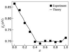
Figure 4: Conductivity activation energy $E_{\rm a}$ of lithium borophosphate glasses with compositions 0.33Li₂O-0.67[$x$B₂O₃-$(1\!-\!x)$P₂O₅] as a function of the borate to phosphate mixing parameter $x$. The symbols refers to experimental data Storek et al. (2012) and the line to the theoretical modelling for parameters $V_{0}=0.64\,$\mathrm{e}\mathrm{V}$$ and $\sigma_{\varepsilon}=0.42$. The theoretical activation energies were calculated in steps $\Delta x=0.04$ for lattices of linear size $L=100\,a$. Averages were performed over 20 disordered energy landscapes (generated as described in Sec. II). The relative standard deviation of the calculated mean $E_{\rm a}$ values does not exceed 0.4%.

For comparison of conductivity data, we need to specify one further parameter. According to Eq. (13), $\sigma_{\rm dc}$ is proportional to $1/L$ and to the attempt frequency $\nu$, which enters the local conductances in Eq. (7) via the hopping rates $w_{i\to j}^{0}$ in Eq. (5). Since $L=N_{L}a$ and the number $N_{L}^{3}$ of sites known in our modelling, the relevant parameter is $\nu/a$. The mean jump distance $a$ can be estimated to be about $5$\AA$$ in the alkali borophosphate glasses, see, for example, Fig. 11 in Ref. Christensen et al. (2013). We fix this value for $a$ (independent of $x$), although the mean jump distance can be expected to vary slightly with $x$. Indeed a weak decrease of $a$ with $x$ has been reported in Ref. Christensen et al. (2013). We note that also the other parameters $V_{0}$ and $\sigma_{\varepsilon}$ should vary with $x$, but our successful modelling of the activation energies with fixed values of $V_{0}$ and $\sigma_{\varepsilon}$ suggests that the variation is weak also.

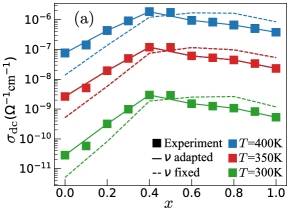
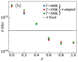
Figure 5: (a) Conductivity $\sigma_{\rm dc}$ of lithium borophosphate glasses with compositions 0.33Li₂O-0.67[$x$B₂O₃-$(1\!-\!x)$P₂O₅] as a function of $x$. The symbols refer to experimental data Storek et al. (2012) and the lines to theoretical calculations for the same parameters $V_{0}$ and $\sigma_{\varepsilon}$ as in Fig. 4. The dashed and solid lines refer to the theoretical modellings with a fixed and with adapted attempt frequencies $\nu$, respectively. (b) Attempt frequencies $\nu$ used for fitting of the conductivity data. The horizontal dashed line marks the fixed, $x$-independent $\nu$ value. The calculations were carried out in steps of $\Delta x=0.2$ for a linear system size $L=35\,a$. Averages were performed over 30 energy landscapes. The relative standard deviation of the calculated mean $\sigma_{\rm dc}$ values does not exceed 15%.

More difficult is to make reasonable assumptions for $\nu$ apart from estimating it to be of the order of optical phonon frequencies. The attempt frequency in particular contains entropic contributions, including a “local migration entropy” not considered in our coarse-grained approach based on a hopping model. This local migration entropy quantifies the mean number of relevant pathways (or typical configuration space) accessible for a mobile ion in a rare transition from one ion site to a neighboring one, which, on a coarse-grained time scale, is described as an instantaneous hopping process.

In view of this complexity, we use two procedures to specify $\nu$. In the first one, we consider also $\nu$ to have a fixed value in order to keep the number of model parameters as small as possible. An interesting question then is, if we can successfully recover the overall change of conductivities with $x$ as found in the experiments. In the second procedure, we adjust $\nu$ to fit the experimental conductivity data for each value of $x$. This can be considered as an “overfitting”, because irrespective of our construction of the underlying energy landscape described in Sec. II, it would be always possible to match the measured data. However, the adapted attempt frequencies should have reasonable values and their variation can provide interesting insights into entropy variations.

Figure 5(a) shows the experimental data for the conductivity (symbols) for three temperatures in comparison with the theoretical modelling for fixed $\nu$ (dashed lines) and adapted $\nu$ (solid lines). The corresponding attempt frequencies are displayed in Fig. 5(b), where the dashed horizontal line marks the fixed, $x$-independent $\nu$ value. From the comparison of the theoretical with the experimental results in Fig. 5(a), we can conclude that the overall variation of $\sigma_{\rm dc}(x)$ is captured by the modelling with a fixed attempt frequency $\nu$, but a quantitative agreement is not obtained. The value $\nu=4\times 10^{14}\,$\mathrm{H}\mathrm{z}$$, found by least squared error fitting of the measured data, has a reasonable order of magnitude.

When adjusting $\nu$ to match the measured data, we find a decrease of the adapted $\nu$ values from values of about $10^{15}\,$\mathrm{H}\mathrm{z}$$ to values of about $10^{14}\,$\mathrm{H}\mathrm{z}$$ when $x$ is increased from zero to one, see Fig. 5(b). All these values are of reasonable order of magnitude. Interestingly, a similar variation of pre-exponential factors from $10^{16}\,$\mathrm{H}\mathrm{z}$$ down to $10^{14}\,$\mathrm{H}\mathrm{z}$$ has been found by fitting NMR spectra Storek et al. (2012).

V.2 Glasses 0.35Na₂O-0.65[$\bm{x}$B₂O₃-$\bm{(1\!-\!x)}$P₂O₅]

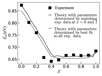
Figure 6: Conductivity activation energy $E_{\rm a}$ of sodium borophosphate glasses with compositions 0.35Na₂O-0.65[$x$B₂O₃-$(1\!-\!x)$P₂O₅] as a function of the borate to phosphate mixing parameter $x$. The symbols refer to experimental data Christensen et al. (2013) and the lines to the theoretical modelling for $V_{0}=0.76\,$\mathrm{e}\mathrm{V}$$ and $\sigma_{\varepsilon}=0.30$ (solid line), and for $V_{0}=0.73\,$\mathrm{e}\mathrm{V}$$ and $\sigma_{\varepsilon}=0.32$ (dashed line). The step size $\Delta x$, system size and disorder averaging used in the calculations are the same as in Fig. 4. The relative standard deviation of the calculated mean $E_{\rm a}$ values does not exceed 0.5% (for both modellings with the different parameter values).

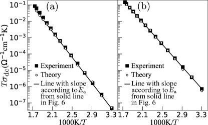
Figure 7: Arrhenius plots of $T\sigma_{\rm dc}$ in sodium borophosphate glasses of compositions (a) 0.35Na₂O-0.65[$0.2$B₂O₃-$0.8$P₂O₅] ($x=0.2$) and (b) 0.35Na₂O-0.65[$0.4$B₂O₃-$0.6$P₂O₅] ($x=0.4$). The filled symbols refer to experimental data Christensen et al. (2013) and the open symbols to a modelling for parameters $V_{0}=0.76\,$\mathrm{e}\mathrm{V}$$ and $\sigma_{\varepsilon}=0.3$, i.e. equal to the ones yielding the solid line in Fig. 6. The attempt frequencies in the calculations are $\nu=5\times 10^{14}\,$\mathrm{H}\mathrm{z}$$ in (a) and $\nu=1.5\times 10^{14}\,$\mathrm{H}\mathrm{z}$$ in (b). The solid lines in (a) and (b) have slopes corresponding to the calculated activation energies in Fig. 6. Values of $T\sigma_{\rm dc}$ were calculated in the interval $303\,$\mathrm{K}$$-$563\,$\mathrm{K}$$ in temperature steps of $20\,$\mathrm{K}$$, and the system size and disorder averaging used in the calculations are the same as in Fig. 5. The relative standard deviation of the calculated mean $\sigma_{\rm dc}$ values does not exceed 23% in (a) and (b).

Figure 6 shows the comparison of the experimental Christensen et al. (2013) (symbols) and modelled conductivity activation energies (solid and dashed lines) for the sodium borophosphate glasses with compositions 0.35Na₂O-0.65[$x$B₂O₃-$(1\!-\!x)$P₂O₅]. When determining the parameters $V_{0}$ and $\sigma_{\varepsilon}$ as for the lithium borophosphate glasses in the previous Sec. V.1, i.e. by requiring the theoretical values to match the experimental ones for $x=0$ and $x=1$, we obtain $V_{0}=0.76\,$\mathrm{e}\mathrm{V}$$ and $\sigma_{\varepsilon}=0.30$. The predicted behaviour for $0<x<1$ is given by the solid line in Fig. 6. The agreement with the experimental data is satisfactory but less good for $x\lesssim 0.5$ than in Fig. 4. As we do not know whether the experimental data for $x=0$ and $x=1$ have less uncertainty than those for $x\neq 0,1$, we determined the parameters $V_{0}$ and $\sigma_{\varepsilon}$ alternatively also by a least squared error fitting of the experimental data. This gives $V_{0}=0.73\,$\mathrm{e}\mathrm{V}$$ and $\sigma_{\varepsilon}=0.32$. The corresponding results are shown as dashed line in Fig. 6. They give a slightly better agreement for $x\lesssim 0.5$, but underestimate the experimental $E_{\rm a}$ values for $x\geq 0.6$.

Moreover, we find that Arrhenius plots of measured conductivity data for $x=0.2$ and $x=0.4$ (filled symbols) can be well described by the hopping model (open symbols) with the parameters $V_{0}=0.76\,$\mathrm{e}\mathrm{V}$$ and $\sigma_{\varepsilon}=0.30$, see Fig. 7. The solid lines in Fig. 7(a) and (b) have slopes that agree with the modelled conductivity activation energies given by the solid line in Fig. 6. This demonstrates that the corresponding $E_{a}$ values can account for the experimental findings also if $x$ is smaller than 0.5. In the further modelling of dc-conductivities, we use the parameter values $V_{0}=0.76\,$\mathrm{e}\mathrm{V}$$ and $\sigma_{\varepsilon}=0.30$.

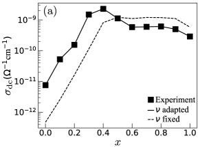
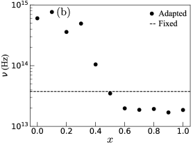
Figure 8: (a) Conductivity $\sigma_{\rm dc}$ of sodium borophosphate glasses with compositions 0.35Na₂O-0.65[$x$B₂O₃-$(1\!-\!x)$P₂O₅]. The symbols refers to experimental data Christensen et al. (2013) and the lines to theoretical calculations for the parameters $V_{0}=0.76\,$\mathrm{e}\mathrm{V}$$ and $\sigma_{\varepsilon}=0.30$, i.e. corresponding to the ones used for the solid line in Fig. 6. The dashed and solid lines refer to the theoretical modelling with a fixed and with adapted attempt frequencies $\nu$, respectively. (b) Attempt frequencies $\nu$ used for fitting of the conductivity data. The horizontal dashed line marks the fixed, $x$-independent $\nu$ value. The calculation were performed in steps of $\Delta x=0.1$ for a system size and a disorder averaging as in Fig, 5. The relative standard deviation of the calculated mean $\sigma_{\rm dc}$ values does not exceed 16%.

Figure 8(a) shows the experimental data for the conductivity (symbols) for three temperatures in comparison with the theoretical modelling for fixed $\nu$ (dashed lines) and adapted $\nu$ (solid lines). The corresponding attempt frequencies are displayed in Figure 8(b). The agreement between experiment and theory is of similar quality as for the lithium borophosphate glasses in Fig. 5 with attempt frequencies having a reasonable order of magnitude.

V.3 Glasses 0.4Na₂O-0.6[$\bm{x}$B₂O₃-$\bm{(1\!-\!x)}$P₂O₅]

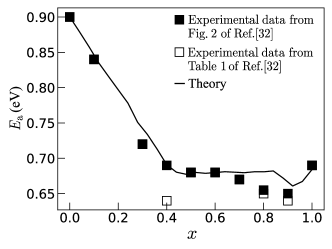
Figure 9: Conductivity activation energy $E_{\rm a}$ of sodium borophosphate glasses with compositions 0.4Na₂O-0.6[$x$B₂O₃-$(1\!-\!x)$P₂O₅]. The filled and open symbols refer to experimental data taken from table 1 and from Fig. 2b) of Ref. Zielniok et al. (2007). The line refers to the theoretical modelling with $V_{0}=0.93\,$\mathrm{e}\mathrm{V}$$ and $\sigma_{\varepsilon}=0.25$. The step size $\Delta x$, system size and disorder averaging used in the calculations are the same as in Figs. 4 and 6. The relative standard deviation of the calculated mean $E_{\rm a}$ values does not exceed 0.5%.

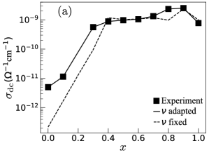
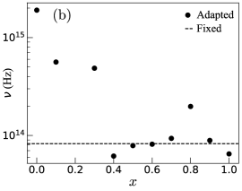
Figure 10: (a) Conductivity $\sigma_{\rm dc}$ of sodium borophosphate glasses with compositions 0.4Na₂O-0.6[$x$B₂O₃-$(1\!-\!x)$P₂O₅]. The symbols refer to experimental data Zielniok et al. (2007) and the lines to theoretical calculations for the same parameters $V_{0}$ and $\sigma_{\varepsilon}$ as in Fig. 9. The dashed and solid lines are for the theoretical modelling with a fixed and with adapted attempt frequencies $\nu$, respectively. (b) Attempt frequencies $\nu$ used for fitting of the conductivity data. The horizontal dashed line marks the fixed, $x$-independent $\nu$ value. Step sizes $\Delta x$, linear system size and disorder averaging are the same as in Fig. 8. The relative standard deviation of the calculated mean $\sigma_{\rm dc}$ values does not exceed 22%.

Figure 9 shows the comparison of the experimental Zielniok et al. (2007) (filled and open symbols) with the calculated conductivity activation energies (solid lines) for sodium borophosphate glasses with compositions 0.4Na₂O-0.6[$x$B₂O₃-$(1\!-\!x)$P₂O₅]. The parameters obtained from matching the measured data at $x=0$ and $x=1$ are $V_{0}=0.93\,$\mathrm{e}\mathrm{V}$$ and $\sigma_{\varepsilon}=0.25$. As can be seen from the figure, the theoretical results again agree well with the experimental findings.

The calculated conductivities $\sigma_{\rm dc}$ in Fig. 10 compare similarly with experimental data as the other glass series shown in Figs. 5 and 8, again with reasonable values of adjusted attempt frequencies in the range $10^{14}-10^{15}\,$\mathrm{H}\mathrm{z}$$.

VI Conclusions

Ionic conductivities $\sigma_{\rm dc}$ and their activation energies $E_{\rm a}$ have been successfully modelled for various alkali borophosphate glasses with compositions $yM_{2}$O-$(1\!-\!y)$[$x$B₂O₃-$(1\!-\!x)$P₂O₅] ($M$: alkali ion, $y$: molar fraction of alkali oxide, $x$: borate to phosphate mixing parameter). This was done based on a construction of site energy landscapes and a hopping model for the alkali ion motion developed in earlier studies Schuch et al. (2011); Bosi et al. (2021). In this model, it was assumed that the Coulomb interaction can be treated in a mean-field like manner and that it can be effectively included into a noise contribution to the site energies, or, more generally speaking, to the jump rates. Whether this is a valid concept needs to be explored, in particular, whether a Coulomb gap must be considered in the one-particle density of states, as it has been studied in the related problem of electron hopping transport in amorphous semiconductors Pollak (1970); Efros and Shklovskii (1975); Möbius et al. (1992); Müller and Pankov (2007).

The energy landscape construction relies on the idea that the countercharges associated with different types of NFUs are important and that changes in the concentrations of NFU types dominate the variation of the energy landscape when the mixing parameter $x$ is altered. Concentrations of the NFU units can be measured by MAS-NMR and Raman spectroscopy and they were successfully described theoretically in the earlier studies by a statistical mechanical approach Schuch et al. (2011); Bosi et al. (2021). Experimental activation energies for compositions with different mixing ratio $x$ could be described quantitatively by introducing one energy scale parameter $V_{0}$ and a parameter $\sigma_{\varepsilon}$ characterising additional noise in the energy landscape. These two parameters were determined by fitting of the experimental results for $x=0$ (alkali borate glass) and $x=1$ (alkali phosphate glass). The $E_{\rm a}$ values calculated for $0<x<1$ are theoretical predictions then.

A modelling of activation energies has been conducted in the earlier studies also, first based on KMC simulations Schuch et al. (2011) and later by the analytical method used here Bosi et al. (2021). In these former calculations, however, local ion jumps could have vanishing energetic barriers, which is an unphysical feature. In the present study we showed that this problem can be resolved when introducing a minimal barrier $u_{0}>0$ for local jumps. Let us mention that a good agreement of the theoretical results with the experimental observations is not achieved if $u_{0}$ becomes too large. We estimated $u_{0}$ by considering it to have values comparable to the thermal energy at the glass transition temperature $T_{\rm g}$. A fixed value $u_{0}$ independent of the borate to phosphate mixing ratio was used for simplicity. One can refine this approach and adjust $u_{0}$ to $T_{\rm g}$. The change of $T_{\rm g}$ with $x$ in general correlates well with the number of bridging oxygens, and this number can be calculated from the known NFU concentrations. It will be interesting to see in the future, how a corresponding refinement modifies the theoretical results. In a further refinement one may consider a distribution of the (lower) barriers for local jumps in addition to the distribution of ion site energies.

Calculations of conductivities for the hopping model were carried out here for the first time based on an analytical theoretical method. The overall variation of measured conductivities was reproduced when taking an $x$-independent attempt frequency $\nu$ in the jump rates of the hopping model. When allowing for a variation of the attempt frequencies with $x$, a quantitative agreement with experimental results was obtained for reasonable values of $\nu$ varying in the range $10^{13}-10^{14}\,$\mathrm{H}\mathrm{z}$$. In the corresponding calculations we considered a mean jump distance of $5\,$Å independent of $x$. Generally, the mean jump distance, the energetic scale parameter $V_{0}$ and the noise strength $\sigma_{\varepsilon}$ can be expected to vary with $x$. However, in order to see whether the theory has predictive power, we kept the number of parameters as small as possible. It is our hope to determine or estimate the parameters $V_{0}$ and $\sigma_{\varepsilon}$ without a fitting in the future by resorting on additional structural information as, e.g., gained from RMC modelling and molecular dynamics simulations.

For extending and refining the modelling, it will be furthermore important to check theoretical predictions for other dynamical probes commonly studied in experiments, such as ac-conductivities and spin lattice relaxation rates Heitjans et al. (2005); Vinod Chandran and Heitjans (2016). This can be done, in principle, by extensive kinetic Monte Carlo simulations Rinn et al. (1998). Whether corresponding calculations can be carried out in a reliable manner also by fast numerical solutions of equations, as done here for dc-conductivities and their activations energies, is an open problem. A recently developed experimental technique is the charge attachment induced ion transport (CAIT) Schäfer and Weitzel (2018); Schäfer et al. (2019); Weitzel (2021), where collective diffusion coefficients of mobile ions are extracted by a modelling of diffusion profiles. A particular merit of the CAIT method is that mobile ions of different types can be directly injected in the glassy phase. This makes it possible that the observed concentration-dependent diffusion coefficients are governed by other intervals of the site energy distribution than those governing dc-conductivities obtained from impedance spectroscopy. Comparison of CAIT results with theoretical calculations will thus provide an important additional means for testing the energy landscape construction.

Acknowledgement
This work has been funded by the Deutsche Forschungsgemeinschaft (DFG, Project No. 428906592). We sincerely thank the members of the DFG Research Unit FOR 5065 for fruitful discussions.

References

- Fergus (2011) J. W. Fergus, “Sensing mechanism of non-equilibrium solid-electrolyte-based chemical sensors,” J. Solid State Electrochem. 15, 971–984 (2011).
- Yoo et al. (2006) S. J. Yoo, J. W. Lim, and Y.-E. Sung, “Improved electrochromic devices with an inorganic solid electrolyte protective layer,” Sol. Energy Mater. Sol. Cells 90, 477–484 (2006).
- Tervonen et al. (2011) A. Tervonen, S. K. Honkanen, and B. R. West, “Ion-exchanged glass waveguide technology: a review,” Opt. Eng. 50, 1 – 16 (2011).
- Samui and Sivaraman (2010) A. Samui and P. Sivaraman, “Solid polymer electrolytes for supercapacitors,” in Polymer Electrolytes, Woodhead Publishing Series in Electronic and Optical Materials, edited by C. Sequeira and D. Santos (Woodhead Publishing, 2010) Chap. 11, pp. 431–470.
- Kim et al. (2015) J. G. Kim, B. Son, S. Mukherjee, N. Schuppert, A. Bates, O. Kwon, M. J. Choi, H. Y. Chung, and S. Park, “A review of lithium and non-lithium based solid state batteries,” J. Power Sources 282, 299–322 (2015).
- Koettgen et al. (2018) J. Koettgen, S. Grieshammer, P. Hein, B. O. H. Grope, M. Nakayama, and M. Martin, “Understanding the ionic conductivity maximum in doped ceria: trapping and blocking,” Phys. Chem. Chem. Phys. 20, 14291–14321 (2018).
- Meyer et al. (1996) M. Meyer, V. Jaenisch, P. Maass, and A. Bunde, “Mixed alkali effect in crystals of - and -alumina structure,” Phys. Rev. Lett. 76, 2338–2341 (1996).
- Dyre et al. (2009) J. C. Dyre, P. Maass, B. Roling, and D. L. Sidebottom, “Fundamental questions relating to ion conduction in disordered solids,” Rep. Prog. Phys. 72, 046501 (2009).
- Maass (1999) P. Maass, “Towards a theory for the mixed alkali effect in glasses,” J. Non-Cryst. Solids 255, 35–46 (1999).
- Hunt (1999) A. G. Hunt, “Mixed-alkali effect: some new results,” J. Non-Cryst. Solids 255, 47–55 (1999).
- Maass et al. (1996) P. Maass, M. Meyer, A. Bunde, and W. Dieterich, “Microscopic explanation of the non-Arrhenius conductivity in glassy fast ionic conductors,” Phys. Rev. Lett. 77, 1528–1531 (1996).
- Baranovskii and Cordes (1999) S. D. Baranovskii and H. Cordes, “On the conduction mechanism in ionic glasses,” J. Chem. Phys. 111, 7546–7557 (1999), https://doi.org/10.1063/1.480081 .
- Dyre and Schrøder (2000) J. C. Dyre and T. B. Schrøder, “Universality of ac conduction in disordered solids,” Rev. Mod. Phys. 72, 873–892 (2000).
- Porto et al. (2000) M. Porto, P. Maass, M. Meyer, A. Bunde, and W. Dieterich, “Hopping transport in the presence of site-energy disorder: Temperature and concentration scaling of conductivity spectra,” Phys. Rev. B 61, 6057–6062 (2000).
- Dieterich and Maass (2002) W. Dieterich and P. Maass, “Non-Debye relaxations in disordered ionic solids,” Chem. Phys. 284, 439–467 (2002).
- Habasaki and Hiwatari (2004) J. Habasaki and Y. Hiwatari, “Molecular dynamics study of the mechanism of ion transport in lithium silicate glasses: Characteristics of the potential energy surface and structures,” Phys. Rev. B 69, 144207 (2004).
- Lammert et al. (2009) H. Lammert, R. D. Banhatti, and A. Heuer, “The cationic energy landscape in alkali silicate glasses: Properties and relevance,” J. Chem. Phys. 131, 224708 (2009).
- Vogel (2004) M. Vogel, “Identification of lithium sites in a model of LiPO3 glass: Effects of the local structure and energy landscape on ionic jump dynamics,” Phys. Rev. B 70, 094302 (2004).
- Adams and Swenson (2000) S. Adams and J. Swenson, “Determining ionic conductivity from structural models of fast ionic conductors,” Phys. Rev. Lett. 84, 4144–4147 (2000).
- Adams and Swenson (2005) S. Adams and J. Swenson, “Bond valence analysis of reverse Monte Carlo produced structural models; a way to understand ion conduction in glasses,” J. Phys.: Condens. Matter 17, S87–S101 (2005).
- Müller et al. (2007) C. Müller, E. Zienicke, S. Adams, J. Habasaki, and P. Maass, “Comparison of ion sites and diffusion paths in glasses obtained by molecular dynamics simulations and bond valence analysis,” Phys. Rev. B 75, 014203 (2007).
- Karlsson et al. (2015) M. Karlsson, M. Schuch, R. Christensen, P. Maass, S. W. Martin, S. Imberti, and A. Matic, “Structural origin of the mixed glass former effect in sodium borophosphate glasses investigated with neutron diffraction and reverse Monte Carlo modeling,” J. Phys. Chem. C 119, 27275–27284 (2015).
- Schuch et al. (2012) M. Schuch, R. Christensen, C. Trott, P. Maass, and S. W. Martin, “Investigation of the structures of sodium borophosphate glasses by reverse Monte Carlo modeling to examine the origins of the mixed glass former effect,” J. Phys. Chem. C 116, 1503–1511 (2012).
- Schuch et al. (2011) M. Schuch, C. Trott, and P. Maass, “Network forming units in alkali borate and borophosphate glasses and the mixed glass former effect,” RSC Adv. 1, 1370–1382 (2011).
- Silver and Bray (1958) A. H. Silver and P. J. Bray, “Nuclear magnetic resonance absorption in glass. i. nuclear quadrupole effects in boron oxide, soda‐boric oxide, and borosilicate glasses,” J. Chem. Phys. 29, 984–990 (1958).
- Eckert (2018) H. Eckert, “Spying with spins on messy materials: 60 years of glass structure elucidation by NMR spectroscopy,” Int. J. Appl. Glass Sci. 9, 167–187 (2018).
- Youngman (2018) R. Youngman, “NMR spectroscopy in glass science: A review of the elements,” Materials 11, 476 (2018).
- Bosi et al. (2021) M. Bosi, J. Fischer, and P. Maass, “Network-forming units, energy landscapes, and conductivity activation energies in alkali borophosphate glasses: Analytical approaches,” J. Phys. Chem. C 125, 6260–6268 (2021).
- Ambegaokar et al. (1971) V. Ambegaokar, B. I. Halperin, and J. S. Langer, “Hopping conductivity in disordered systems,” Phys. Rev. B 4, 2612–2620 (1971).
- Dörfler and Bullo (2013) F. Dörfler and F. Bullo, “Kron reduction of graphs with applications to electrical networks,” IEEE Trans. Circuits Syst. I Regul. Pap. 60, 150–163 (2013).
- Zielniok et al. (2007) D. Zielniok, C. Cramer, and H. Eckert, “Structure property correlations in ion-conducting mixed-network former glasses: Solid-state NMR studies of the system Na2O-B2O3-P2O5,” Chem. Mat. 19, 3162–3170 (2007).
- Rinke and Eckert (2011) M. T. Rinke and H. Eckert, “The mixed network former effect in glasses: solid state nmr and xps structural studies of the glass system (Na2O)x(BPO4)1-x,” Phys. Chem. Chem. Phys. 13, 6552–6565 (2011).
- Larink et al. (2012) D. Larink, H. Eckert, M. Reichert, and S. W. Martin, “Mixed network former effect in ion-conducting alkali borophosphate glasses: Structure/property correlations in the system [M2O]1/3[(B2O3)x(P2O5)]2/3 (M=Li, K, Cs),” J. Phys. Chem. C 116, 26162–26176 (2012).
- Peibst et al. (2005) R. Peibst, S. Schott, and P. Maass, “Internal friction and vulnerability of mixed alkali glasses,” Phys. Rev. Lett. 95, 115901 (2005).
- Maass and Peibst (2006) P. Maass and R. Peibst, “Ion diffusion and mechanical losses in mixed alkali glasses,” J. Non-Cryst. Solids 352, 5178–5187 (2006).
- Note (2) More precisely, we view it to give a mean-field contribution in the equivalent vacancy picture of the dynamics, as described in Ref. Bosi et al. (2021).
- Metropolis et al. (1953) N. Metropolis, A. W. Rosenbluth, M. N. Rosenbluth, A. H. Teller, and E. Teller, “Equation of state calculations by fast computing machines,” J. Chem. Phys. 21, 1087–1092 (1953).
- Note (3) What is truly relevant for the following theory too be valid is that the field-perturbed rates satisfy ). This can be interpreted as a kind of local detailed balance condition in the linear response limit.
- Hoshen and Kopelman (1976) J. Hoshen and R. Kopelman, “Percolation and cluster distribution. I. Cluster multiple labeling technique and critical concentration algorithm,” Phys. Rev. B 14, 3438–3445 (1976).
- Note (4) As for the dimensions of the vectors they are: for , , and and for . For the matrices the dimensions are for , , and , for and , and for . The matrices and are the transpose of and , respectively.
- Storek et al. (2012) M. Storek, R. Böhmer, S. W. Martin, D. Larink, and H. Eckert, “NMR and conductivity studies of the mixed glass former effect in lithium borophosphate glasses,” J. Chem. Phys. 137, 124507 (2012).
- Christensen et al. (2013) R. Christensen, G. Olson, and S. W. Martin, “Ionic conductivity of mixed glass former 0.35Na2O+0.65[B2O3+P2O5] glasses,” J. Phys. Chem. B 117, 16577–16586 (2013).
- Pollak (1970) M. Pollak, “Effect of carrier-carrier interactions on some transport properties in disordered semiconductors,” Discuss. Faraday Soc. 50, 13–19 (1970).
- Efros and Shklovskii (1975) A. L. Efros and B. I. Shklovskii, “Coulomb gap and low temperature conductivity of disordered systems,” J. Phys. C: Solid State Phys. 8, L49–L51 (1975).
- Möbius et al. (1992) A. Möbius, M. Richter, and B. Drittler, “Coulomb gap in two- and three-dimensional systems: Simulation results for large samples,” Phys. Rev. B 45, 11568–11579 (1992).
- Müller and Pankov (2007) M. Müller and S. Pankov, “Mean-field theory for the three-dimensional Coulomb glass,” Phys. Rev. B 75, 144201 (2007).
- Heitjans et al. (2005) P. Heitjans, S. Indris, and M. Wilkening, “Solid-state diffusion and NMR,” Diffusion Fundamentals 2, 45 (2005).
- Vinod Chandran and Heitjans (2016) C. Vinod Chandran and P. Heitjans, “Chapter one - Solid-state NMR studies of lithium ion dynamics across materials classes,” (Academic Press, 2016) pp. 1–102.
- Rinn et al. (1998) B. Rinn, W. Dieterich, and P. Maass, “Stochastic modelling of ion dynamics in complex systems: dipolar effects,” Phil. Mag. B 77, 1283–1292 (1998).
- Schäfer and Weitzel (2018) M. Schäfer and K.-M. Weitzel, “Site energy distribution of ions in the potential energy landscape of amorphous solids,” Mater. Today Phys. 5, 12–19 (2018).
- Schäfer et al. (2019) M. Schäfer, D. Budina, and K.-M. Weitzel, “Site energy distribution of sodium ions in a sodium rubidium borate glass,” Phys. Chem. Chem. Phys. 21, 26251–26261 (2019).
- Weitzel (2021) K.-M. Weitzel, “Charge attachment–induced transport – Toward new paradigms in solid state electrochemistry,” Curr. Opin. Electrochem. 26, 100672 (2021).