Functional model for generalised resolvents and its application to time-dispersive media

Abstract

Motivated by recent results concerning the asymptotic behaviour of differential operators with highly contrasting coefficients, which have involved effective descriptions involving generalised resolvents, we construct the functional model for a typical example of the latter. This provides a spectral representation for the generalised resolvent, which can be utilised for further analysis, in particular the construction of the scattering operator in related wave propagation setups.

In memoriam Sergey Naboko

1 From resonant composites to generalised resolvents

Recent advances in the multiscale analysis of differential equations modelling heterogeneous media with high contrast (“high contrast homogenisation”) have shown that when the contrast between the material properties of individual components is scaled appropriately with the typical size of heterogeneity (e.g. period in the case of periodic media), the effective description exhibits frequency dispersion ( i.e. the dependence of the wavelength on frequency) or, equivalently in the time domain, a memory-type effect with a convolution kernel, see [73, 74, 18, 14, 16, 17]. From the physical perspective, the mentioned effect can be viewed as the result of a resonant behaviour of one of the components of such a composite medium, when the typical length-scale of waves (in the case of an unbounded medium) or eigenmodes (in the case of a bounded region) is comparable to the typical size of heterogeneity.

The need to quantify this effect for various classes of boundary value problems (BVP), which ultimately aims at addressing the effect of the underlying miscrosopic resonance on the overall behaviour of a class of physical systems, has also motivated the development of functional analytic frameworks for the analysis of wave scattering and effects of length-scale interactions for parameter-dependent BVP, see [19, 20, 21, 22]. The approach of the latter works was inspired by a treatment of BVP going back to the so-called Birman-Kreĭn-Vishik methodology [9, 40, 41, 72] and its recent development by Ryzhov [64], rooted in an earlier construction of the functional model of perturbation theory by one of the authors [44, 45]. The theory of boundary triples, which was introduced in [31, 24, 37, 38], provides a convenient functional analytic framework for the implementation of the ideas introduced by Birman, Kreĭn, and Vishik, as shown in a number of parallel recent developments [32, 34, 6, 30, 64, 12]; see also the seminal contributions by Calkin [13], Boutet de Monvel [10], Birman and Solomyak [11], Grubb [33], and Agranovich [3].

In the process of the analysis of BVP using the Ryzhov’s method, the link between the resonant behaviour of high-contrast media and the additional dependence on the spectral parameter (in comparison to the “standard” situation of moderate contrast) has become clear, as one establishes an expression of the generalised-resolvent type for the operator on the resonant component. Indeed, one effect of the high contrast on material properties is to force the solution gradients (corresponding to e.g. the strain tensor in elasticity) to nearly vanish on the component with a large value of the material parameter (such as an elastic modulus). The resulting “effective” description is exactly of the kind that has appeared in the analysis of time-dispersive media [27, 28].

The operator-theoretic study of generalised resolvents was initiated by Neumark [48, 49], who established that they form exactly the class of mappings obtained by “truncating” the resolvent of a self-adjoint operator in an “out-of space extension” of the original Hilbert space. These results were generalised by Štraus [68, 69, 67], who also developed a procedure for the construction of the associated spectral function and introduced the notion of a characteristic function of a generalised resolvent (“Štraus characteristic function”), which provides for an implicit link to scattering theory for problems with impedance-type boundary conditions, i.e. those that contain a non-constant function of the spectral parameter $z$ (which represents the square of frequency in the context of wave propagation). In the context of Sturm-Liouville problems, impedance-type problems have been studied independently by Shkalikov [66].

Following an analogy with the connection between the characteristic function of Lifshitz [43] and the spectral form of the functional model for dissipative operator due to Pavlov [53], as well as its implications for scattering theory due to Adamyan, Arov, and Pavlov [1, 2], it appears natural to pose the question of the construction of the functional model for generalised resolvents, its relationship with the the characteristic function of Štraus, and the implications of this construction for the scattering theory for impedance-type BVP. Furthermore, in relation to the kind of generalised impedance problems that emerge in the context of resonant homogenisation, it seems natural to also explore appropriate analogues of Pavlov’s model of potentials of zero radius with internal structure [55, 56], resulting in an explicit description of a class of generalised resolvents quantifying the interactions between the resonant and non-resonant parts of the medium. To the best of our knowledge, the present work is the first step in implementing the above programme.

2 Motivation for the problem to be analysed

For differentiation $\partial$ and $\tau\in[-\pi,\pi),$ consider the he operator ${\partial_{\tau}}:=\partial+{\rm i}\tau.$ Problems of multiscale analysis of the behaviour of heterogeneous media with high contrast lead to differential operators on an interval $(0,l)$ of the form

$$A\left(\begin{array}[]{c}u\\ \beta\end{array}\right)=\left(\begin{array}[]{c}-\partial_{\tau}^{2}u\\[1.99997pt] -\eta^{-1}Du+\gamma\eta^{-2}\beta\end{array}\right),$$ (1)

where $\gamma>0$, $\eta\in{\mathbb{R}},$ $\omega\in{\mathbb{C}},$ $|\omega|=1,$ and

$$Du:={\partial_{\tau}}u(0)-\omega{\partial_{\tau}}u(l).$$ (2)

The domain of the operator $A$ in $L^{2}(0,l)\oplus{\mathbb{C}}$ is defined as follows:

$${\rm dom}(A)=\left\{\left(\begin{array}[]{c}u\\[1.99997pt] \beta\end{array}\right)\in W^{2}_{2}(0,l)\oplus{\mathbb{C}}:\ u(0)=\omega u(l),\ \eta u(0)=\beta\right\}.$$ (3)

The pair $(u,\beta)^{\top}$ describes the approximation of the solution to a second-order differential equation with contrasting parameters in a “resonant” asymptotic regime, see our recent papers [15, 17] as well as [16] for a similar object in the PDE context.

The components $u$ and $\beta$ correspond to the leading-order behaviour on the “soft” (resonant) and “stiff” parts of the composite medium, capturing the fact that the soft part supports vibrations of relatively small wavelengths in relation to the stiff part. We next describe the context in which (1) emerges in more detail.

2.1 The operator $A$ as the dilation of a generalised resolvent

The operator (1)–(3) is the Štraus-Neumark dilation for the solution operator ${\mathcal{R}}(z)$ of the problem

$$-\partial_{\tau}^{2}u-zu=f,$$ (4)

$$u(0)=\omega u(l),\qquad Du=(\gamma-\eta^{2}z)u(0),$$

where the relationship between $u(0)$ (and hence $u(l)$) to $\beta$ given in (3) has been used. Its action is the composition of the solution to

$$A\left(\begin{array}[]{c}u\\ \beta\end{array}\right)-z\left(\begin{array}[]{c}u\\ \beta\end{array}\right)=\left(\begin{array}[]{c}f\\ 0\end{array}\right),$$

and the projection $P_{\widetilde{H}}$ onto $\widetilde{H}:=L^{2}(0,l)\oplus\{0\}.$ On the abstract level, this is expressed as follows:

$${\mathcal{R}}(z)=P_{\widetilde{H}}(A-zI)^{-1}\bigr{|}_{\widetilde{H}},$$ (5)

where $\widetilde{H}$ is identified with $L^{2}(0,l),$ and therefore in the terminology introduced by [48, 68], the operator ${\mathcal{R}}(z)$ is a generalised resolvent.

Note that in the boundary-value problem (4) the spectral parameter is present not only in the differential equation but also in the boundary conditions. In fact, (4) can be written in the form

$$\widetilde{A}_{\text{\rm max}}u-zu=f,\qquad\widetilde{\Gamma}_{1}u=B(z)\widetilde{\Gamma}_{0}u,\quad\qquad u\in W^{2,2}(0,l),$$ (6)

where $\widetilde{A}_{\rm max}$ is the operator generated by the differential expression $\partial_{\tau}^{2}$ on the domain $W^{2,2}(0,l),$ appropriately chosen operators $\widetilde{\Gamma}_{0},$ $\widetilde{\Gamma}_{1}:W^{2,2}(0,l)\to{\mathbb{C}}^{2}$ satisfy the Green’s identity for all $u,v\in W^{2,2}(0,l):$

$$\int_{0}^{l}\bigl{(}-\partial_{\tau}^{2}u\overline{v}+u\overline{\partial_{\tau}^{2}v}\bigr{)}\equiv\bigl{\langle}\widetilde{A}_{\rm max}u,v\bigr{\rangle}_{L^{2}(0,l)}-\bigl{\langle}u,\widetilde{A}_{\rm max}v\bigr{\rangle}_{L^{2}(0,l)}=\bigl{\langle}\widetilde{\Gamma}_{1}u,\widetilde{\Gamma}_{0}v\bigr{\rangle}_{{\mathbb{C}}^{2}}-\bigl{\langle}\widetilde{\Gamma}_{0}u,\widetilde{\Gamma}_{1}v\bigr{\rangle}_{{\mathbb{C}}^{2}},$$

and $-B(z)$ is an operator-valued $R$-function, i.e. $B(z)$ is analytic in $\mathbb{C}_{+}\cup\mathbb{C}_{-}$ with $\Im z\Im B(z)\leq 0.$ The abstract result of [68] ensures that the solution to any boundary-value problem with this property is a generalised resolvent, i.e. it admits a representation of the form (6). Thus the link between (1)–(3) and (5) (hence (4)) is a particular example of a general result of Neumark and Štraus. On the other hand, problems of both types (6) and (1)–(3) emerge in the process of deriving operator-norm asymptotic approximations for problems of high contrast (“resonant”) homogenisation [15, 17]. In particular, the problem (4) emerges from the asymptotic analysis of the generalised resolvent obtained by projecting the original operator onto the soft component, whereas the problem (1)–(3) turns out to be (up to a unitary equivalence) the asymptotic limit of the family of the complete operator resolvents. While on the abstract level it is not possible to show that the convergence of the generalised resolvents implies the convergence of their Neumark-Štraus dilations, this happens to be the case in all setups of interest in homogenisation.

Over the recent years there have been several attempts to provide an explicit construction of the Neumark-Štraus dilation for several classes of generalised resolvents; among the relevant works we would like to point out [66, 7, 8, 27, 28]. This activity has been motivated by the growing interest to the mathematical analysis of highly dispersive media. However, all these constructions stop short of obtaining the functional model representation for the said dilation.

On the other hand, in many physically relevant contexts, including that of homogenisation, families of generalised resolvents emerge in a natural way for which the asymptotic expansion with respect to the (small) length-scale parameter yields a leading-order term that can be represented by a generalised resolvent with a linear dependence on the spectral parameter $z.$ From the physics perspective, this corresponds to an effective model of the medium that includes zero-range potentials with an internal structure [2, 55]. It can be argued that the linearity of the impedance in $z$ is essentially equivalent to the model where these zero-range potentials represent point dipoles [18]. If one takes into account higher-order terms in the mentioned asymptotic expansion, one is able to pass from dipole models of effective media to more general multipole ones. While in the present work we focus on the dipole case, the development of the general multipole theory is extremely topical from the point of view of describing metamaterials and can be treated on the basis of the mathematical approach presented here, with a natural replacement of the scalar model by a matrix one.

In summary, the “dipole” homogenisation regime offers a simple, yet physically relevant in certain frequency regimes, model for which the construction of the dilation can be carried our explicitly, by essentially adding a one-dimensional subspace.

This suggests, in particular, that the formulation (4) is of a generic type, applicable to a variety of physical contexts, including the Maxwell system of electromagnetism and linearised elasticity. We anticipate that in all those setups it will yield new interesting physical and mathematical effects, which, in our opinion, vindicates our interest to such a simple-looking boundary-value problem as (4).

Next, we look at the associated operator $A$ in more detail.

2.2 Infinite-graph setup and Gelfand transform

Consider a graph ${\mathbb{G}}_{\infty},$ periodic in one direction, so that ${\mathbb{G}}_{\infty}+\ell={\mathbb{G}}_{\infty},$ where $\ell$ is a fixed vector, which defines the graph axis. Let the periodicity cell ${\mathbb{G}}_{\varepsilon}$ be a finite compact graph of total length $\varepsilon\in(0,1),$ and denote by $e_{j},$ $j=1,2,\dots n,$ $n\in{\mathbb{N}},$ its edges. For each $j=1,2,\dots,n,$ we identify $e_{j}$ with the interval $[0,\varepsilon l_{j}],$ where $\varepsilon l_{j}$ is the length of $e_{j}.$ We associate with the graph ${\mathbb{G}}_{\infty}$ the Hilbert space

$$L_{2}({\mathbb{G}}_{\infty}):=\bigoplus\limits_{{\mathbb{Z}}}\bigoplus\limits_{j=1}^{n}L_{2}(0,\varepsilon l_{j}).$$

Consider a family $\{A^{\varepsilon}\}_{\varepsilon>0}$ of operators in $L_{2}({\mathbb{G}}_{\infty}),$ generated by second-order differential expressions $-a^{\varepsilon}\partial^{2},$ with positive ${\mathbb{G}}_{\varepsilon}$-periodic coefficients $a^{\varepsilon}$ on ${\mathbb{G}}_{\infty},$ and defined on the domain ${\rm dom}(A^{\varepsilon})$ describing the “natural” coupling conditions at the vertices of ${\mathbb{G}}_{\infty}:$

$${\rm dom}(A^{\varepsilon})=\Bigl{\{}u\in\bigoplus\limits_{e\in{\mathbb{G}}_{\infty}}W^{2,2}\bigl{(}e):\ u\text{\ continuous,}\ \sum_{e\ni V}\sigma_{e}a^{\varepsilon}u^{\prime}(V)=0\ \ \forall V\in{\mathbb{G}}_{\infty}\Bigr{\}}.$$ (7)

In (7) the summation is carried out over the edges $e$ sharing the vertex $V,$ the coefficient $(a^{\varepsilon})^{2}$ in the vertex condition is calculated on the edge $e,$ and $\sigma_{e}=-1$ or $\sigma_{e}=1$ for $e$ incoming or outgoing for $V,$ respectively. The matching conditions (7) represent the combined conditions of continuity of the function and of vanishing sums of its co-normal derivatives at all vertices (i.e. the so-called Kirchhoff conditions).

Applying to the operators $A^{\varepsilon}$ a suitable version of the Gelfand transform [29], one obtains a two-parametric family of operators $A^{\varepsilon}_{\tau},$ $\tau\in[-\pi,\pi),$ $\varepsilon>0$ defined on the space of $L^{2}$-functions on a “unit cell” $\mathbb{G}$ of size one, obtained from the “$\varepsilon$-cell” ${\mathbb{G}}_{\varepsilon}$ by a simple scaling ${\mathbb{G}}_{\varepsilon}\ni x\mapsto y=x/\varepsilon\in{\mathbb{G}}.$ More precisely, there exists a unimodular list $\{w_{V}(e)\}_{e\ni V},$ cf. [15], defined at each vertex $V$ of ${\mathbb{G}}$ as a finite collection of values corresponding to the edges adjacent to $V$. For each $\tau\in[-\pi,\pi)$, the fibre operator $A^{\varepsilon}_{\tau}$ is generated by the differential expression $a^{\varepsilon}\varepsilon^{-2}\partial_{\tau}^{2}$ on the domain

$${\rm dom}(A^{\varepsilon}_{\tau})=\Big{\{}v\in\bigoplus\limits_{e\in{\mathbb{G}}}W^{2,2}\bigl{(}e): \ w_{V}(e)v|_{e}(V)=w_{V}(e^{\prime})v|_{e^{\prime}}(V)\text{\ for all }e,e^{\prime}\text{ adjacent to }V,$$

$$\sum_{e\ni V}\widetilde{\partial}_{\tau}v(V)=0\ \ \ {\rm for\ each\ vertex}\ V\Big{\}},$$

where $\widetilde{\partial}_{\tau}v(V)$ stands for “the weighted co-derivative” $\sigma_{e}w_{V}(e)a^{\varepsilon}\varepsilon^{-2}\partial_{\tau}v$ of the function $v$ on the edge $e,$ calculated at the vertex $V.$

2.3 An example of operator on a graph and it norm-resovent approximation

The periodic graph considered, its periodicity cell and the result of Gelfand transform is shown in Fig. 1. Denote by $a_{j},$ $j=1,2,3,$ the values of $a^{\varepsilon}$ on the edges $e_{j},$ $j=1,2,3,$ and assume for simplicity that $a_{j}=1.$

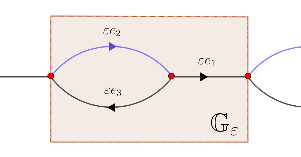
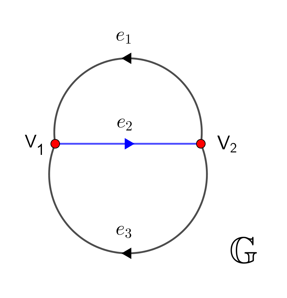
Figure 1: Example of a periodic graph with contrast. The infinite graph $\mathbb{G}_{\infty}$ and the “period” $\mathbb{G}_{\varepsilon}$ are outlined on the left; the graph unit cell $\mathbb{G}$ obtained after applying the Gelfand transform is shown on the right. The soft component is drawn in blue.

The unimodular functions $w_{V_{k}}(e_{j}),$ $j=1,2,3,$ $k=1,2,$ are then chosen as follows:

$$\begin{gathered}\{w_{V_{1}}(e_{j})\}_{j=1}^{3}=\bigl{\{}1,1,{\rm e}^{{\rm i}\tau(l_{2}+l_{3})}\bigr{\}},\quad\{w_{V_{2}}(e_{j})\}_{j=1}^{3}=\bigl{\{}{\rm e}^{{\rm i}\tau l_{3}},1,1\bigr{\}}\end{gathered}$$

For all $\tau\in[-\pi,\pi),$ consider an operator $\mathcal{A}_{\rm hom}^{\tau}$ on $L^{2}(0,l_{2})\oplus\mathbb{C},$ defined as follows. Denote

$$\xi_{\tau}=-\frac{a_{1}}{l_{1}}{\rm e}^{{\rm i}\tau(l_{1}+l_{3})}-\frac{a_{3}}{l_{3}}{\rm e}^{-{\rm i}\tau l_{2}}.$$

The domain $\operatorname{dom}(\mathcal{A}_{\text{\rm hom}}^{\tau})$ is set to be

$$\operatorname{dom}\bigl{(}\mathcal{A}_{\text{\rm hom}}^{\tau}\bigr{)}=\biggl{\{}(u,\beta)^{\top}\in L^{2}(0,l_{2})\oplus\mathbb{C}:\ u\in W^{2,2}(0,l_{2}),\ u(0)=-\frac{\overline{\xi}_{\tau}}{|\xi_{\tau}|}u(l_{2})=\frac{\beta}{\sqrt{l_{1}+l_{3}}}\biggr{\}}.$$

On $\operatorname{dom}(\mathcal{A}_{\text{\rm hom}}^{\tau})$ the action of the operator is set by

$$\mathcal{A}_{\text{\rm hom}}^{\tau}\binom{u}{\beta}=\left(\begin{array}[]{c}-\partial_{\tau}^{2}u\\[8.00003pt] -\dfrac{1}{\sqrt{l_{1}+l_{3}}}\biggl{(}{\partial_{\tau}}u(0)+\dfrac{\overline{\xi}_{\tau}}{|\xi_{\tau}|}\partial_{\tau}u(l_{2})\biggr{)}+\bigl{(}l_{1}+l_{3}\bigr{)}^{-1}\biggl{(}\dfrac{l_{1}}{a_{1}}+\dfrac{l_{3}}{a_{3}}\biggr{)}^{-1}\biggl{(}\dfrac{\tau}{\varepsilon}\biggr{)}^{2}\beta\end{array}\right).$$

Theorem 2.1 ([17]).

Denote $H:=\oplus_{j=1}^{3}L^{2}(0,l_{j}).$ There exists $C>0,$ independent of $\varepsilon$ and $\tau,$ such that

$$\bigl{\|}(A_{\varepsilon}^{\tau}-z)^{-1}-\Psi^{*}(\mathcal{A}_{\text{\rm hom}}^{\tau}-z)^{-1}\Psi\bigr{\|}_{H\to H}=C\varepsilon^{2},$$

where $\Psi$ is a partial isometry from $H$ to $L^{2}(0,l_{2})\oplus\mathbb{C}.$

Clearly the operator $A_{\text{\rm hom}}^{\tau}$ is of the form (1)–(3) with

$$l=l_{2},\quad\eta=\sqrt{l_{1}+l_{3}},\quad\gamma=(l_{1}a_{1}^{-1}+l_{3}a_{3}^{-1})^{-1}(\tau/\varepsilon)^{2},\quad\omega=-\overline{\xi}_{\tau}/|\xi_{\tau}|.$$ (8)

2.4 Abstract boundary triples

Our approach is based on the theory of boundary triples [31, 37, 38, 24], applied to the class of operators introduced above. We next recall two fundamental concepts of this theory, namely the boundary triple and the generalised Weyl-Titchmarsh matrix function.

Definition 2.1.

Suppose that ${A}_{\rm max}$ is the adjoint to a densely defined symmetric operator ${A}_{\rm min}$ on a separable Hilbert space ${H}$ (“physical region space”) and that ${\Gamma}_{0},$ ${\Gamma}_{1}$ are linear mappings of ${\rm dom}({A}_{\max})\subset{H}$ to a separable Hilbert space ${\mathcal{H}}$ (“boundary space”).

A. The triple $({\mathcal{H}},{\Gamma}_{0},{\Gamma}_{1})$ is called a boundary triple for the operator ${A}_{\max}$ if:

1. For all $u,v\in{\rm dom}({A}_{\max})$ one has the second Green’s identity

   $$\langle{A}_{\max}u,v\rangle_{{H}}-\langle u,{A}_{\max}v\rangle_{{H}}=\langle{\Gamma}_{1}u,{\Gamma}_{0}v\rangle_{{\mathcal{H}}}-\langle{\Gamma}_{0}u,{\Gamma}_{1}v\rangle_{{\mathcal{H}}}.$$

2. The mapping ${\rm dom}({A}_{\max})\ni u\longmapsto({\Gamma}_{0}u,{\Gamma}_{1}u)\in{{\mathcal{H}}}\oplus{{\mathcal{H}}}$ is onto.

B. The operator-valued Herglotz function ${\mathfrak{m}}={\mathfrak{m}}(z),$ defined by

$${\mathfrak{m}}(z){\Gamma}_{0}u_{z}={\Gamma}_{1}u_{z},\ \ u_{z}\in\ker({A}_{\max}-z),\ \ z\in\mathbb{C}_{+}\cup{\mathbb{C}}_{-},$$ (9)

is referred to as the $M$-function of the operator ${A}_{\max}$ with respect to the triple $({\mathcal{H}},{\Gamma}_{0},{\Gamma}_{1})$.

C. A non-trivial extension ${A}_{B}$ of the operator ${A}_{\min}$ such that ${A}_{\min}\subset{A}_{B}\subset{A}_{\max}$ is called almost solvable if there exists a boundary triple $({\mathcal{H}},{\Gamma}_{0},{\Gamma}_{1})$ for ${A}_{\max}$ and a bounded linear operator $B$ defined on ${\mathcal{H}}$ such that for every $u\in{\rm dom}({A}_{\max})$ one has $u\in{\rm dom}({{A}_{B}})$ if and only if ${\Gamma}_{1}u=B{\Gamma}_{0}u.$

In what follows, we use the boundary triple approach to the extension theory of symmetric operators with equal deficiency indices (see [25] for a review of the subject), which is particularly useful in the study of extensions of ordinary differential operators of second order.

2.5 The boundary triple for the prototype operator

Here we aim at constructing a convenient boundary triple for the operator (1), (3) in the space $H:=L^{2}(0,l)\oplus{\mathbb{C}}.$ To this end, consider the following domains for the minimal and maximal (i.e. the adjoint to the minimal) operators corresponding to the same expression (1):

$${\rm dom}\left(A_{\rm min}\right) =\left\{\left(\begin{array}[]{c}u\\ \beta\end{array}\right)\in W^{2}_{2}(0,l)\oplus{\mathbb{C}}:u(0)=\omega u(l)=\eta^{-1}\beta,\ Du=0\right\},$$ (12)

$${\rm dom}\left(A_{\rm max}\right) =\left\{\left(\begin{array}[]{c}u\\ \beta\end{array}\right)\in W^{2}_{2}(0,l)\oplus{\mathbb{C}}:u(0)=\omega u(l)\right\},$$ (15)

where $Du$ is defined by (2).

Theorem 2.2.

The triple $({\mathcal{H}},\Gamma_{0},\Gamma_{1}),$ where

$$\mathcal{H}:=\mathbb{C},\qquad\Gamma_{0}\left(\begin{array}[]{c}u\\ \beta\end{array}\right):=Du,\qquad\Gamma_{1}\left(\begin{array}[]{c}u\\ \beta\end{array}\right):=\frac{\beta}{\eta}-u(0),\quad\qquad\left(\begin{array}[]{c}u\\ \beta\end{array}\right)\in W^{2}_{2}(0,l)\oplus{\mathbb{C}},$$ (16)

is a boundary triple for the operator $A_{\rm max}$ defined by the expression (1) on the domain (15).

Proof.

The second property of the triple in Definition 2.1 is verified immediately, and the following calculations show that the second Green’s identity holds as well:

$$\left\langle A_{\rm max}\left(\begin{array}[]{c}u\\ \beta\end{array}\right),\left(\begin{array}[]{c}v\\ \zeta\end{array}\right)\right\rangle_{H}-\left\langle\left(\begin{array}[]{c}u\\ \beta\end{array}\right),A_{\rm max}\left(\begin{array}[]{c}v\\ \zeta\end{array}\right)\right\rangle_{H}=$$

$$=-\int\limits_{0}^{l}\partial_{\tau}^{2}u\bar{v}dx-\left(\frac{1}{\eta}Du+\frac{\gamma}{\eta^{2}}\beta\right)\bar{\zeta}+\int\limits_{0}^{l}u\overline{\partial_{\tau}^{2}v}dx+\beta\overline{\left(\frac{1}{\eta}Dv+\frac{\gamma}{\eta^{2}}\zeta\right)}$$

$$=-\int\limits_{0}^{l}u\overline{\partial_{\tau}^{2}v}dx+\left[u\overline{{\partial_{\tau}}v}-{\partial_{\tau}}u\overline{v}\right]_{0}^{l}-\left(\frac{1}{\eta}Du+\frac{\gamma}{\eta^{2}}\beta\right)\overline{\zeta}+\int\limits_{0}^{l}u\overline{\partial_{\tau}^{2}v}dx+\beta\overline{\left(\frac{1}{\eta}Dv+\frac{\gamma}{\eta^{2}}\zeta\right)}$$

$$=\left(u(l)\overline{{\partial_{\tau}}v(l)}-u(0)\overline{{\partial_{\tau}}v(0)}\right)-\left({\partial_{\tau}}u(l)\overline{v(l)}-{\partial_{\tau}}u(0)\overline{v(0)}\right)+\frac{\beta}{\eta}\overline{Dv}-\frac{\bar{\zeta}}{\eta}Du$$

$$=\Gamma_{1}\left(\begin{array}[]{c}u\\ \beta\end{array}\right)\overline{\Gamma_{0}\left(\begin{array}[]{c}v\\ \zeta\end{array}\right)}-\Gamma_{0}\left(\begin{array}[]{c}u\\ \beta\end{array}\right)\overline{\Gamma_{1}\left(\begin{array}[]{c}v\\ \zeta\end{array}\right)}.$$

∎

Let us next calculate the corresponding $M$-function, which is defined by the property (cf. (9))

$${\mathfrak{m}}(z)\Gamma_{0}\left(\begin{array}[]{c}u_{z}\\ \beta_{z}\end{array}\right)=\Gamma_{1}\left(\begin{array}[]{c}u_{z}\\ \beta_{z}\end{array}\right),\qquad\quad\left(\begin{array}[]{c}u_{z}\\ \beta_{z}\end{array}\right)\in\ker(A_{\rm max}-zI).$$

Theorem 2.3.

The $M$-function of the operator $A_{\max}$ with respect to the triple (16) is given by

$${\mathfrak{m}}(z)=-\frac{\sin\sqrt{z}l}{2k\bigl{(}\Re({\rm e}^{{\rm i}\tau l}\bar{\omega})-\cos\sqrt{z}l\bigr{)}}-\frac{1}{\eta^{2}z-\gamma}.$$ (17)

Proof.

The general solution of the spectral problem

$$\left\{\begin{array}[]{ll}-\partial_{\tau}^{2}u_{z}=zu_{z},\\[3.99994pt] -\eta^{-1}Du+\gamma\eta^{-2}\beta_{z}=z\beta_{z},\end{array}\right.$$

is given by

$$u_{z}={\rm e}^{-{\rm i}\tau x}\bigl{(}C_{1}{\rm e}^{{\rm i}\sqrt{z}x}+C_{2}{\rm e}^{-{\rm i}\sqrt{z}x}\bigr{)},\qquad\beta_{z}=\dfrac{\eta}{\eta^{2}z-\gamma}Du,$$

where the branch of the square root is chosen so that $\sqrt{z}$ is real for real positive $z$.

Normalising $u_{z}$ by the condition

$$u_{z}(0)=\omega u_{z}(l)=1,$$ (18)

we obtain $\Gamma_{0}u_{z}=Du_{z}$, $\Gamma_{1}u_{z}=\eta^{-1}\beta_{z}-1,$ and hence

$${\mathfrak{m}}(z)=\frac{\Gamma_{1}u_{z}}{\Gamma_{0}u_{z}}=-\frac{1}{\eta^{2}z-\gamma}-\frac{1}{Du_{z}}.$$ (19)

It remains to determine the values $C_{1},$ $C_{2}$ for $u_{z}$ satisfying (18) and hence evaluate $Du_{z}.$ To this end we write

$$u_{z}(0)=C_{1}+C_{2}=1,\qquad\quad u_{z}(l)={\rm e}^{-{\rm i}\tau l}\bigl{(}C_{1}{\rm e}^{{\rm i}\sqrt{z}l}+C_{2}{\rm e}^{-{\rm i}\sqrt{z}l}\bigr{)}=\bar{\omega},$$

whence

$$C_{1}=\dfrac{\bar{\omega}{\rm e}^{{\rm i}\tau l}-{\rm e}^{-{\rm i}\sqrt{z}l}}{2{\rm i}\sin\sqrt{z}l},\qquad\quad C_{2}=\frac{{\rm e}^{{\rm i}\sqrt{z}l}-\bar{\omega}{\rm e}^{{\rm i}\tau l}}{2{\rm i}\sin(\sqrt{z}l)}.$$

It follows that

$$u_{z}(x)=\frac{{\rm e}^{-{\rm i}\tau x}}{\sin\sqrt{z}l}\left(\bar{\omega}e^{{\rm i}\tau l}\sin\sqrt{z}x+\sin\sqrt{z}(l-x)\right),\qquad x\in[0,l],$$

and, in particular,

$$Du_{z}=\frac{\sqrt{z}}{\sin\sqrt{z}l}\left(\bar{\omega}{\rm e}^{{\rm i}\tau l}-\cos\sqrt{z}l-\omega(\bar{\omega}\cos\sqrt{z}l-{\rm e}^{-{\rm i}\tau l})\right)=\frac{2\sqrt{z}\bigl{(}\Re({\rm e}^{{\rm i}\tau l}\bar{\omega})-\cos\sqrt{z}l)\bigr{)}}{\sin\sqrt{z}l}.$$

Combining this with (19) finally yields (17). ∎

3 Spectral form of the functional model for the Štraus-Neumark dilation

The first (and the only known to us) attempt at a construction of the functional model for a generalised resolvent is contained in [57], where a “5-component” self-adjoint dilation was developed for a (actually, more challenging) problem with an impedance linear in $\sqrt{z}$ rather than $z,$ using methods resembling those employed in the dilation theory for dissipative operators. However that work stops short of constructing any sort of spectral representation for the named dilation.

Setting out to construct a spectral form for the dilation in our case, we draw our inspiration in essentially the same pool of ideas but, instead of constructing a 5-component model like in [57], we achieve our goal in two steps. First, facilitated by the linear in $z$ form of the impedance, we construct an out-of-space self-adjoint extension of the associated symmetric operator (i.e. a symmetric obtained by “restricting” the generalised resolvent), so that the named extension is the Neumark-Štraus dilation of our generalised resolvent. Second, considering a fixed dissipative extension of the same symmetric operator, we develop its self-adjoint dilation, thereby dilating the underlying space even further. Following this, we utilise an explicit formula describing the resolvent of the Neumark-Štraus dilation constructed at the first step in this ”twice-dilated” space. The overall success of the strategy is rooted in the fact that the self-adjoint dilation of the dissipative operator introduced at the second step admits an explicit spectral representation. It is in this spectral representation that the action of the self-adjoint Neumark-Štraus dilation takes the simplest form, which can be shown to be a triangular perturbation of a Toeplitz operator [36, 21]. The latter is then used to pass over to a yet another representation, where the original Hilbert space is unitarily equivalent to a space of the class $K_{\theta},$ which has been studied in e.g. [23, 5, 58, 59, 46].

Finally, we make use of the fact that the space $K_{\theta},$ in its turn, is unitarily equivalent to the $L^{2}$-space over a Clark measure. We note that alternative constructions to [57] have appeared in the literature [66, 7, 8, 27, 28], which, however, touches neither upon the spectral form of the Neumark-Štraus dilation nor upon the functional model for the associated generalised resolvent.

The first step of the above programme has been carried out in Section 2.5, where the corresponding extension of the minimal symmetric operator has been constructed, the corresponding boundary triple framework has been developed, and the corresponding $M$-function has been computed.

In order to pursue the second step, we now need to pick a convenient dissipative operator belonging to the class considered, which is the class of all extensions $A_{\varkappa},$ $\varkappa\in{\mathbb{C}},$ of $A_{\rm min}$ whose domains are given on the basis of the boundary triple $({\mathbb{C}},\Gamma_{1},\Gamma_{0})$ for $A_{\rm max}$ as follows:

$$\operatorname{dom}(A_{\varkappa}):=\bigl{\{}f\in\operatorname{dom}(A_{\max}):\Gamma_{1}f=\varkappa\Gamma_{0}f\bigr{\}}.$$ (20)

It follows from [37, Thm. 2] and [31, Chap. 3 Sec. 1.4] (see also an alternative formulation in [62, Thm. 1.1], and [65, Sec. 14]) that $A_{\varkappa}$ is maximal, i. e., $\rho(A_{\varkappa})\neq\emptyset$. For the construction of the Pavlov model, we need to consider one selected dissipative operator, given by (20) with $\varkappa={\rm i}.$

It was shown by Ryzhov [62] that the characteristic function ${\mathfrak{s}}$ of Štraus for the operator $A_{{\rm i}}$ is given by

$${\mathfrak{s}}(z)=1-\frac{2{\rm i}}{{\rm i}+{\mathfrak{m}}(z)},\qquad z\in\mathbb{C}_{+}.$$ (21)

Thus, the characteristic function is the Cayley transform of the $M$-function ${\mathfrak{m}},$ cf. [51]. Based on the material presented in Section 2.5 or by a standard argument, one verifies that $\mathfrak{s}$ is analytic in $\mathbb{C}_{+}$ and, for each $z\in\mathbb{C}_{+}$, $\left|\mathfrak{s}\right|\leq 1$. Therefore, by invoking the classical Fatou theorem, see e.g. [70], the function $\mathfrak{s}$ has at least nontangential limits almost everywhere on the real line which we will henceforth denote by $\mathfrak{s}(k),$ $k\in{\mathbb{R}}.$ However, in our case its analytic properties in the vicinity of the real line are in fact much better, which we discuss and take advantage of below.

The next definitions apply to arbitrary values of $\varkappa,$ although in our analysis we will require the objects pertaining to $\varkappa=0$ and $\varkappa={\rm i}.$ We abbreviate

$$\theta_{\varkappa}(z): =1-2({\rm i}-\mathfrak{m}(z))^{-1}\chi_{\varkappa}^{+}\,,\qquad z\in\mathbb{C}_{-},$$

$$\widehat{\theta}_{\varkappa}(z): =1-2({\rm i}+\mathfrak{m}(z))^{-1}\chi_{\varkappa}^{-}\,,\qquad z\in\mathbb{C}_{+},$$

where

$$\chi_{\varkappa}^{\pm}:=\frac{1\pm\varkappa}{2},$$ (22)

The definition of the characteristic ${\mathfrak{s}}$ and the fact that $\mathfrak{m}$ is a Herglotz function [35] allow us to write $\theta_{\varkappa}(z)$ and $\widehat{\theta}_{\varkappa}(z)$ in terms of $\mathfrak{s}$ as follows:

$$\theta_{\varkappa}(z) =1+(\overline{\mathfrak{s}(\overline{z})}-1)\chi_{\varkappa}^{+},\quad\quad\,z\in\mathbb{C}_{-},$$ (23)

$$\widehat{\theta}_{\varkappa}(z) =1+(\mathfrak{s}(z)-1)\chi_{\varkappa}^{-},\quad\quad\,\,z\in\mathbb{C}_{+}.$$

We will next use an explicit construction of the functional model for the operator family $A_{\varkappa},$ introduced in [53, 52, 54] and further developed in [45, 63, 61, 71]. As the objects introduced above, it applies to arbitrary values of $\varkappa,$ although henceforth we only utilise it for the case $\varkappa=0.$

Our immediate goal is to represent the self-adjoint dilation [70] of the dissipative operator $A_{\rm i}$ as the operator of multiplication. To this end, one first constructs a three-component model of the dilation, following Pavlov’s procedure [52, 53, 54] and then explicitly defines a unitary mapping to the so-called “symmetric” representation ${\mathfrak{H}}$ of the dilation. Namely, one starts with the Hilbert space

$$\mathscr{H}=L^{2}(\mathbb{R}_{-})\oplus H\oplus L^{2}(\mathbb{R}_{+}),$$

and the self-adjoint operator ${\mathcal{A}}$ in $\mathscr{H}$ such that

$$P_{H}(\mathscr{A}-zI)^{-1}\upharpoonright_{H}=(A_{{\rm i}}-zI)^{-1}\,,\qquad z\in\mathbb{C}_{-}.$$

Then, as in the case of additive non-selfadjoint perturbations [45], it is established [62, Thm. 2.3] that there exists an isometry $\Phi:\mathscr{H}\to{\mathfrak{H}}$ such that

$$\Phi(\mathscr{A}-zI)^{-1}=(\cdot-z)^{-1}\Phi.$$

Next, we shall recall how this construction is made explicit in our particular case.

Following the argument of [45, Thm. 1], it is shown in [62, Lem. 2.4] that

$$\Gamma_{0}(A_{{\rm i}}-\cdot I)^{-1}h\in H_{-}^{2}\quad\text{and}\quad\Gamma_{0}(A_{{\rm i}}^{*}-\cdot I)^{-1}h\in H_{+}^{2},$$ (24)

where $H_{\pm}^{2}$ are the standard Hardy classes, see e.g. [60, Sec. 4.8]. Further, for a two-component vector function $(\widetilde{g},g)^{\top}$ taking values in $\mathbb{C}^{2}=\mathbb{C}\oplus\mathbb{C}$, one considers the integral

$$\int_{\mathbb{R}}\left\langle\begin{pmatrix}1&\overline{\mathfrak{s}(s)}\\ \mathfrak{s}(s)&1\end{pmatrix}\binom{\widetilde{g}(s)}{g(s)},\binom{\widetilde{g}(s)}{g(s)}\right\rangle_{\mathbb{C}^{2}}ds,$$ (25)

which is nonnegative, due to the contractive properties of $\mathfrak{s}$. The space

$$\mathfrak{H}:=L^{2}\Biggl{(}\mathbb{C}^{2};\begin{pmatrix}1&\overline{\mathfrak{s}}\\ \mathfrak{s}&1\end{pmatrix}\Biggr{)}$$

is the completion of the linear set of two-component vector functions $(\widetilde{g},g)^{\top}:{\mathbb{R}}\to\mathbb{C}^{2}$ in the norm (25), factored with respect to vectors of zero norm. Naturally, not every element of the set can be identified with a pair $(\widetilde{g},g)^{\top}$ of two independent functions. Still, in what follows we keep the notation $(\widetilde{g},g)^{\top}$ for the elements of this space.

Another consequence of the contractive properties of the characteristic function ${\mathfrak{s}}$ is that for $\widetilde{g},g\in L^{2}(\mathbb{R})$ one has

$$\left\|\binom{\widetilde{g}}{g}\right\|_{\mathfrak{H}}\geq\max\bigl{\{}\left\|\widetilde{g}+\overline{\mathfrak{s}}g\right\|_{L^{2}(\mathbb{R})},\\ \left\|\mathfrak{s}\widetilde{g}+g\right\|_{L^{2}(\mathbb{R})}\bigr{\}}.$$

Thus, for every Cauchy sequence $\{({g}_{n},g_{n})^{\top}\}_{n=1}^{\infty}$, with respect to the $\mathfrak{H}$-topology, such that $\widetilde{g}_{n},g_{n}\in L^{2}(\mathbb{R})$ for all $n\in\mathbb{N}$, the limits of $\widetilde{g}_{n}+\overline{\mathfrak{s}}g_{n}$ and $\mathfrak{s}\widetilde{g}_{n}+g_{n}$ exist in $L^{2}(\mathbb{R})$, so that $g_{-}:=\widetilde{g}+\overline{\mathfrak{s}}g$ and $g_{+}:={\mathfrak{s}}\widetilde{g}+g$ can always be treated as $L^{2}(\mathbb{R})$ functions.

Consider the following orthogonal subspaces of $\mathfrak{H}:$

$$D_{-}:=\begin{pmatrix}0\\[1.99997pt] {H}^{2}_{-}\end{pmatrix}\,,\quad D_{+}:=\begin{pmatrix}{H}^{2}_{+}\\[1.99997pt] 0\end{pmatrix}\,.$$

We define the space

$$K:=\mathfrak{H}\ominus(D_{-}\oplus D_{+}),$$

which is characterised as follows (see e.g. [52, 54]):

$$K=\left\{\begin{pmatrix}\widetilde{g}\\ g\end{pmatrix}\in\mathfrak{H}:g_{-}\in{H}^{2}_{-}\,,g_{+}\in{H}^{2}_{+}\right\}\,.$$

The orthogonal projection $P_{K}$ onto the subspace $K$ is given by (see e.g. [44])

$$P_{K}\begin{pmatrix}\widetilde{g}\\ g\end{pmatrix}=\begin{pmatrix}\widetilde{g}-P_{+}{g_{-}}\\[3.00003pt] g-P_{-}g_{+}\end{pmatrix},$$

where $P_{\pm}$ are the orthogonal Riesz projections in $L^{2}(\mathbb{R})$ onto ${H}^{2}_{\pm}$.

The next theorem is a particular case of [20], which generalises [62, Thm. 2.5], and its form is similar to [45, Thm. 3], which treats the case of additive perturbation (cf. [47, 62, 61, 63] for the case of possibly non-additive perturbations).

Theorem 3.1.

Let $R_{\varkappa}(z):=(A_{\varkappa}-zI)^{-1}$ for $z\in\rho(A_{\varkappa})$.

1. If $z\in\mathbb{C}_{-}\cap\rho(A_{\varkappa})$ and $(\widetilde{g},g)^{\top}\in K$, then

   $$\Phi R_{\varkappa}(z)\Phi^{*}\binom{\widetilde{g}}{g}=P_{K}\frac{1}{\cdot-z}\binom{\widetilde{g}}{g-\chi_{\varkappa}^{+}\theta^{-1}_{\varkappa}(z)g_{-}(z)}\,.$$ (26)

2. If $z\in\mathbb{C}_{+}\cap\rho(A_{\varkappa})$ and $(\widetilde{g},g)^{\top}\in K$, then

   $$\Phi R_{\varkappa}(z)\Phi^{*}\binom{\widetilde{g}}{g}=P_{K}\frac{1}{\cdot-z}\binom{\widetilde{g}-\chi_{\varkappa}^{-}\widehat{\theta}^{-1}_{\varkappa}(z)g_{+}(z)}{g}\,.$$ (27)

   Here, ${g_{\pm}}(z)$ denote the values at $z$ of the analytic continuations of the functions $g_{\pm}\in H_{\pm}^{2}$ into the corresponding half-plane.

In the work [36], concerning the matrix model for non-selfadjoint operators with almost Hermitian spectrum, it is shown (see [36, Theorem 3.3]) that provided ${\mathfrak{s}}$ is an inner function (which is precisely the case we are dealing with in the present paper), the Hilbert space $H$ is unitary equivalent to the spaces

$$K_{\mathfrak{s}}:=H_{+}^{2}\ominus{\mathfrak{s}}H^{2}_{+},\qquad K^{\dagger}_{\mathfrak{s}}:=H_{-}^{2}\ominus\overline{\mathfrak{s}}H^{2}_{-}.$$

The related unitary mappings are provided by the formulae (cf. (24))

$$H \ni v\mapsto-\frac{1}{\sqrt{\pi}}\Gamma_{0}(A_{\rm i}-\cdot)^{-1}v=g_{+}\in K_{\mathfrak{s}},$$ (28)

$$H \ni v\mapsto-\frac{1}{\sqrt{\pi}}\Gamma_{0}(A_{-{\rm i}}-\cdot)^{-1}v=g_{-}\in K^{\dagger}_{\mathfrak{s}}.$$

Also note that the unitary equivalence between $K_{\mathfrak{s}}$ $K^{\dagger}_{\mathfrak{s}}$ can be obtained via the element-wise equality

$$K_{\mathfrak{s}}={\mathfrak{s}}K^{\dagger}_{\mathfrak{s}},$$

where it is understood that the multiplication by ${\mathfrak{s}}$ is applied to the traces of $K_{\mathfrak{s}},K^{\dagger}_{\mathfrak{s}},$ see also the corresponding statement pertaining to operators of boundary-value problems for PDEs in [21].

4 Explicit functional model representation

This section contains the main results of the paper, namely the construction of an explicit functional model for the operators $A_{\varkappa},$ i.e. a representation of the Hilbert space $H$ as a space of square summable functions over a measure with respect to which the operator is the multiplication by the independent variable.

We start by noticing that [36, Theorem 3.3] provides a description of the original Hilbert space $H,$ via its unitary equivalence to each of the two spaces $K_{\mathfrak{s}},$ $K^{\dagger}_{\mathfrak{s}}.$ In our particular setup of extensions of minimal symmetric operators, this unitary equivalence is provided by the formulae (28).

We then use the representation of the inner product in $H$ in terms of the resolvent $R_{\varkappa}(z)$ via contour integration in the vicinity of the real line. Using the formulae (26)–(27) and passing to the limit as the contour approaches a sum of integrals over the real line, we obtain one of the measures introduced in [23, 5] (“Alexandrov-Clark measures”) and subsequently studied in [58]; see also the survey [59] and a recent development [42]. In our context, this measure emerges from the Nevanlinna representation of the $M$-function ${\mathfrak{m}}.$

We note that the resolvent representation provided by Theorem 3.1 can be shown to yield that $R_{0}(z)$ is the resolvent of a rank-one self-adjoint perturbation of a Toeplitz operator [36], and thus the original argument of Clark [23], leading to the emergence of Aleksandrov-Clark measures and the functional model for the operator family $A_{\varkappa},$ applies in our case. From this point of view, one can see the argument of the present section and Section 5 as an independent proof of Clark’s theorem, providing a straightforward and explicit formulae for the unitary operators mapping the original Hilbert space $H$ to the functional model. Although, for the reasons given above, the results to follow are not new on the abstract level, they yield an explicit functional model construction in terms of the objects naturally associated with the operator under consideration.

4.1 Construction of a Clark-type measure for the model representation

Suppose that $\varkappa\in{\mathbb{R}}.$ For $\delta>0$ and $N\in{\mathbb{R}}_{+}$ that does not belong to the spectrum of the operator $A_{\varkappa},$ denote by $\Gamma_{\delta,N}$ the boundary of the rectangle

$$\{\zeta\in{\mathbb{C}}:|\Re\zeta|<N,\ |\Im\zeta|<\delta\}$$ (29)

and by $P_{N}$ the spectral projection for $A_{\varkappa}$ onto the interval $[-N,N].$ We also use the shorthand $u_{N}=P_{N}u$ for all $u\in H.$

According to the Dunford-Riesz functional calculus [26, Section XV.5], one has, for all $\delta>0,$

$$P_{N}=-\frac{1}{2\pi{\rm i}}\ointctrclockwise_{\Gamma_{\delta,N}}R_{\varkappa}(\lambda)d\lambda=\frac{1}{2\pi{\rm i}}\ointclockwise_{\Gamma_{\delta,N}}R_{\varkappa}(\lambda)d\lambda,$$ (30)

where $\Gamma_{\delta,N}$ is traced anticlockwise in the first integral in (30) and clockwise in the second integral in (30). Notice that $P_{N}\to I$ in the sense of strong operator convergence. In what follows, we use the notation

$$t:=\lambda-{\rm i}\delta=\Re\lambda\in\mathbb{R}.$$ (31)

On the basis of (30), one has that the following analogue of the inverse Cauchy-Stieltjes formula:

$$\left\langle u_{N},v_{N}\right\rangle_{H}=\frac{1}{2\pi{\rm i}}\int^{N}_{-N}\left\langle(R_{\varkappa}(\lambda)-R_{\varkappa}(\overline{\lambda}))u,v\right\rangle_{H}dt+o(1),\qquad\forall u,v\in H,$$ (32)

where the term $o(1)$ goes to zero as $\delta\to 0$ uniformly in $N.$

Assuming $(\widetilde{g},g)^{\top},(\widetilde{f},f)^{\top}\in K$, we set $u=\Phi^{*}(\widetilde{g},g)^{\top}$ and $v=\Phi^{*}(\widetilde{g},g)^{\top}$ and, using Theorem 3.1 for $\lambda\in{\mathbb{C}}_{+},$ write

$$\left\langle(R_{\varkappa}(\lambda)-R_{\varkappa}(\overline{\lambda}))u,v\right\rangle_{H}=\left\langle P_{K}\frac{1}{\cdot-\lambda}\binom{\widetilde{g}-\chi_{\varkappa}^{-}\widehat{\theta}^{-1}_{\varkappa}(\lambda)g_{+}(\lambda)}{g},\left(\begin{array}[]{c}\tilde{f}\\ f\end{array}\right)\right\rangle_{\mathfrak{H}}$$ (35)

$$-\left\langle P_{K}\frac{1}{\cdot-\overline{\lambda}}\left(\begin{array}[]{c}\tilde{g}\\ g-\chi_{\varkappa}^{+}\theta_{\varkappa}^{-1}(\lambda)g_{-}(\lambda)\end{array}\right),\left(\begin{array}[]{c}\tilde{f}\\ f\end{array}\right)\right\rangle_{\mathfrak{H}}$$ (40)

$$\hskip 170.71652pt=\left\langle\left(\frac{1}{\cdot-\lambda}-\frac{1}{\cdot-\overline{\lambda}}\right)\left(\begin{array}[]{c}\tilde{g}\\ g\end{array}\right)\left(\begin{array}[]{c}\tilde{f}\\ f\end{array}\right)\right\rangle_{\mathfrak{H}}-\mathcal{G}(\lambda,\overline{\lambda}),$$ (45)

where

$$\mathcal{G}(\lambda,\overline{\lambda}) :=\int_{\mathbb{R}}\frac{1}{k-\lambda}\chi_{\varkappa}^{-}\widehat{\theta}_{\varkappa}^{-1}(\lambda)g_{+}(\lambda)\overline{f_{-}(k)}dk-\int_{\mathbb{R}}\frac{1}{k-\overline{\lambda}}\chi_{\varkappa}^{+}\theta_{\varkappa}^{-1}(\overline{\lambda})g_{-}(\overline{\lambda})\overline{f_{+}(k)}dk$$ (46)

$$=2\pi{\rm i}\bigl{\{}\chi_{\varkappa}^{-}\widehat{\theta}_{\varkappa}^{-1}(\lambda)g_{+}(\lambda)\overline{f_{-}(\overline{\lambda})}+\chi_{\varkappa}^{+}\theta_{\varkappa}^{-1}(\overline{\lambda})g_{-}(\overline{\lambda})\overline{f_{+}(\lambda)}\bigr{\}}.$$

For the second equality in (46) we have used the fact that for $h\in H^{\pm}_{2}$ the following identities hold:

$$\int_{\mathbb{R}}\frac{h(k)}{k-z}dk=\pm 2\pi{\rm i}h(z),\qquad z\in\mathbb{C}^{\pm}.$$ (47)

Taking into account (31), the first term on the right-hand side of (45) can be written as follows:

$$\left\langle\left(\frac{1}{\cdot-\lambda}-\frac{1}{\cdot-\overline{\lambda}}\right)\left(\begin{array}[]{c}\tilde{g}\\ g\end{array}\right),\left(\begin{array}[]{c}\tilde{f}\\ f\end{array}\right)\right\rangle_{\mathfrak{H}}=\int_{-\infty}^{\infty}\frac{2{\rm i}\delta}{(k-t)^{2}+\delta^{2}}\mathcal{F}(k)dk,$$ (48)

where

$$\mathcal{F}(k):=\left\langle\left(\begin{array}[]{cc}1&\overline{\mathfrak{s}(k)}\\ \mathfrak{s}(k)&1\end{array}\right)\left(\begin{array}[]{c}\tilde{g}(k)\\ g(k)\end{array}\right),\left(\begin{array}[]{c}\tilde{f}(k)\\ f(k)\end{array}\right)\right\rangle_{{\mathbb{C}}^{2}}.$$

Now, integrating (48) with respect to $t\in[-N,N]$ (where $t$ and $\lambda$ are related via (31)), one obtains

$$\begin{split}\int_{-N}^{N}\biggl{\langle}&\left(\frac{1}{\cdot-\lambda}-\frac{1}{\cdot-\overline{\lambda}}\right)\left(\begin{array}[]{c}\tilde{g}\\ g\end{array}\right),\left(\begin{array}[]{c}\tilde{f}\\ f\end{array}\right)\biggr{\rangle}_{\mathfrak{H}}dt=\frac{1}{2\pi{\rm i}}\int_{-N}^{N}\int_{-\infty}^{\infty}\frac{2{\rm i}\delta}{(k-t)^{2}+\delta^{2}}\mathcal{F}(k)dkdt\\[3.99994pt] &=\int\limits_{-N}^{N}\mathcal{F}(k)\int\limits_{-N}^{N}\frac{\delta}{\pi}\frac{1}{(k-t)^{2}+\delta^{2}}dtdk+o(1)=\int\limits_{-N}^{N}g_{+}(k)\overline{f_{+}(k)}dk+o(1).\end{split}$$ (49)

Now, in view of (45), we rewrite (32) by substituting (46) and (49) into it:

$$\left\langle u_{N},v_{N}\right\rangle_{H}=\int\limits_{-N}^{N}g_{+}(k)\overline{f_{+}(k)}dk-\int\limits_{-N}^{N}\left(\chi_{\varkappa}^{-}\widehat{\theta}_{\varkappa}^{-1}(\lambda)g_{+}(\lambda)\overline{f_{-}(\overline{\lambda})}+\chi_{\varkappa}^{+}\theta_{\varkappa}^{-1}(\overline{\lambda})g_{-}(\overline{\lambda})\overline{f_{+}(\lambda)}\right)dt+o(1).$$

Consider a region $\Omega\subset{\mathbb{C}}$ containing the real line that has no poles or zeros of ${\mathfrak{s}}.$ This is possible due to the fact that $A_{\rm min}$ is simple. Indeed, the operator $A_{\rm i}$ is completely non-selfadjoint and dissipative, which prevents it from having real eigenvalues. This, in turn, ensures that the zeros (and hence the poles as well) of ${\mathfrak{s}}$ are also away from the real line, as they coincide with the spectrum of $A_{\rm i}$ (and its adjoint, respectively).

Furthermore, for each $N$ as above, choose $\delta_{N}$ so that $\Gamma_{\delta,N}\subset\Omega$ for all $\delta<\delta_{N},$ where $\delta$ is defined in (29) and is related to $\lambda$ via (31). In the context of the present paper, we are interested in the member of the family $A_{\varkappa}$ that corresponds to the value $\varkappa=0,$ which we assume to be selected from now on. However, we mention that the argument to follow can be extended to work with other real values of $\varkappa$ as well.

Setting $\varkappa=0$ and taking into account (22) and (23), one obtains

$$\left\langle u_{N},v_{N}\right\rangle_{H} =\int\limits_{-N}^{N}g_{+}(k)\overline{f_{+}(k)}dk-\int\limits_{-N}^{N}\left(\frac{g_{+}(\lambda)\overline{f_{-}(\overline{\lambda})}}{1+\mathfrak{s}(\lambda)}+\frac{g_{-}(\overline{\lambda})\overline{f_{+}(\lambda)}}{1+\overline{\mathfrak{s}(\lambda)}}\right)dt+o(1)$$

$$=\int\limits_{-N}^{N}g_{+}(k)\overline{f_{+}(k)}dk-\int\limits_{-N}^{N}\left(\frac{\mathfrak{s}(\lambda)g_{+}(\lambda)\overline{f_{+}(\lambda)}}{1+\mathfrak{s}(\lambda)}+\frac{\overline{\mathfrak{s}(\lambda)}g_{+}(\lambda)\overline{f_{+}(\lambda)}}{1+\overline{\mathfrak{s}(\lambda)}}\right)dt+o(1),$$

where for the last equality we have used the identities

$$h_{-}(z) =\overline{{\mathfrak{s}}(\overline{z})}h_{+}(\overline{z}),\qquad z\in{\mathbb{C}}_{-},$$ (50)

$$h_{+}(z) ={\mathfrak{s}}(z)h_{-}(\overline{z}),\qquad z\in{\mathbb{C}}_{+},$$

obtained by analytic continuation into $\Omega.$ Furthermore, noticing that

$$\frac{{\mathfrak{s}}}{1+{\mathfrak{s}}}=1-\frac{1}{1+{\mathfrak{s}}},$$ (51)

we rewrite (75) as follows:

$$\langle u_{N},v_{N}\rangle_{H} -\int_{-N}^{N}g_{+}(t)\overline{f_{+}(t)}dt$$

$$=-\int\limits_{-N}^{N}\biggl{\{}g_{+}(\lambda)\overline{f_{+}(\lambda)}-\frac{1}{1+{\mathfrak{s}}(\lambda)}g_{+}(\lambda)\overline{f_{+}(\lambda)}+\frac{\overline{{\mathfrak{s}}(\lambda)}}{1+\overline{{\mathfrak{s}}(\lambda)}}g_{+}(\lambda)\overline{f_{+}(\lambda)}\biggr{\}}dt+o(1)$$

$$=-\int_{N}^{N}g_{+}(t)\overline{f_{+}(t)}dt+\int\limits_{-N}^{N}\biggl{\{}\frac{1}{1+{\mathfrak{s}}(\lambda)}-\frac{\overline{{\mathfrak{s}}(\lambda)}}{1+\overline{{\mathfrak{s}}(\lambda)}}\biggr{\}}g_{+}(t)\overline{f_{+}(t)}dt+o(1).$$

Using the identity

$$\frac{\overline{{\mathfrak{s}}(\lambda)}}{1+\overline{{\mathfrak{s}}(\lambda)}}=\frac{1}{\overline{{\mathfrak{s}}(\lambda)}^{-1}+1}=\frac{1}{{\mathfrak{s}}(\overline{\lambda})+1},\qquad\lambda\in{\mathbb{C}}_{+}.$$ (52)

we therefore have

$$\langle u_{N},v_{N}\rangle_{H}=\int\limits_{-N}^{N}\biggl{\{}\frac{1}{1+{\mathfrak{s}}(\lambda)}-\frac{1}{1+{\mathfrak{s}}(\overline{\lambda})}\biggr{\}}g_{+}(t)\overline{f_{+}(t)}dt$$ (53)

Finally, we combine this with the representation

$$\frac{1}{1+{\mathfrak{s}}(\lambda)}=\frac{1}{2}\biggl{(}1+\frac{\rm i}{{\mathfrak{m}}(\lambda)}\biggr{)}=C_{0}+C_{1}\lambda-\frac{\rm i}{2}\int_{\mathbb{R}}\biggl{(}\frac{1}{\sigma-\lambda}-\frac{\sigma}{1+\sigma^{2}}\biggr{)}d\mu(\sigma)$$ (54)

where $C_{0},C_{1}\in{\mathbb{C}},$ and $\mu$ is the measure of the Nevanlinna representation of the Herglotz function $-{\mathfrak{m}}^{-1},$ see e.g. [60, Section 5.3]. The formula (54) implies, in particular, that

$$\frac{1}{1+\mathfrak{s}(\lambda)}-\frac{1}{1+\mathfrak{s}(\overline{\lambda})}=-\frac{\rm i}{2}\int\limits_{\mathbb{R}}\frac{2{\rm i}\delta d\mu(\sigma)}{(\sigma-t)^{2}+\delta^{2}}=\pi\mathfrak{P}_{\delta}(\mu)(t),$$ (55)

where $\mathfrak{P}_{\delta}$ stands for the Poisson transformation. Next, note that $\mu$ is a Clark measure [5], due to (55) and the identity

$$\frac{1}{1+\mathfrak{s}(\lambda)}-\frac{1}{1+\mathfrak{s}(\overline{\lambda})}=\Re\frac{1-{\mathfrak{s}}(\lambda)}{1+{\mathfrak{s}}(\lambda)},\qquad\lambda\in{\mathbb{C}}_{+},$$

obtained directly from (52).

Substituting (55) into (53) and taking into account the weak*-convergence [39, VI Sec. B] of the Poisson transformations ${\mathfrak{P}}_{\delta}$ as well as the regularity [46] of functions in $K_{\mathfrak{s}}$ guaranteed by the analytic properties of ${\mathfrak{s}}$ discussed above, we pass to the limit as $\delta\to 0$ in (53), to obtain

$$\langle u_{N},v_{N}\rangle=\pi\int_{-N}^{N}g_{+}(t)\overline{f_{+}(t)}d\mu(t)+o(1).$$

Finally, passing to the limit in the last identity as $N\to\infty$ and using the fact that $u_{N}\to u,$ $v_{N}\to v$ yields

$$\langle u,v\rangle=\pi\int_{-\infty}^{\infty}g_{+}(t)\overline{f_{+}(t)}d\mu(t),\qquad u,v\in H.$$

We have thus established the following theorem.

Theorem 4.1.

The Hilbert space $H$ is isometric to the space $L_{2}\bigl{(}\mathbb{R},\pi d\mu\bigr{)},$ where the measure $\mu$ is given by (55). This isometry is the composition of the first formula in (28) and the embedding of $K_{\mathfrak{s}}$ into $L_{2}\bigl{(}\mathbb{R},\pi d\mu\bigr{)}.$ The latter embedding is realised by taking the boundary values on the real line of functions in $K_{\mathfrak{s}},$ which exist $d\mu$-almost everywhere.

Remark 1.

A. Unlike in [23], here the Clark measure $d\mu$ emerges in the context of extensions of symmetric operators, via the operators of the functional model.

B. Theorem 4.1 admits an alternative proof by combining classical results by Clark [23], concerning the isometry between $K_{\mathfrak{s}}$ and $L_{2}\bigl{(}\mathbb{R},\pi d\mu\bigr{)},$ and by Poltoratski [58] (see also the survey [59]), concerning the realisation of the mentioned isometry via passing to the boundary values on the real line.

4.2 The resolvent as an operator of multiplication by the independent variable

Fix $\varkappa\in{\mathbb{R}},$ $z\in{\mathbb{C}}^{+}\cup{\mathbb{C}}^{-},$ and consider $\delta\in(0,|\Im z|)$ and $N\in{\mathbb{R}}$ as described at the beginning of Section 4.1. Similarly to the above, we write

$$R_{\varkappa}(z)P_{N}=-\frac{1}{2\pi{\rm i}}\ointctrclockwise_{\Gamma_{\delta,N}}(z-\lambda)^{-1}R_{\varkappa}(\lambda)d\lambda=\frac{1}{2\pi{\rm i}}\ointclockwise_{\Gamma_{\delta,N}}(z-\lambda)^{-1}R_{\varkappa}(\lambda)d\lambda,$$ (56)

where $\Gamma_{\delta,N}$ is the boundary of the rectangle (29) and the integrals are understood in the same sense as (30). Using (56), we can write

$$\bigl{\langle}R_{\varkappa}(z)u_{N},v_{N}\bigr{\rangle}_{H}=\frac{1}{2\pi{\rm i}}\int\limits^{N}_{-N}\bigl{\langle}\bigl{\{}(z-\lambda)^{-1}R_{\varkappa}(\lambda)-(z-\overline{\lambda})^{-1}R_{\varkappa}(\overline{\lambda})\bigr{\}}u,v\bigr{\rangle}_{H}dt\qquad\forall u,v\in H.$$ (57)

Assuming $(\tilde{g},g)^{\top},$ $(\tilde{f},f)^{\top}\in K$, let $u=\Phi^{*}(\tilde{g},g)^{\top}$ and $v=\Phi^{*}(\tilde{f},f)^{\top}.$ Then one has (cf. (45))

$$\bigl{\langle}\bigl{\{}(z -\lambda)^{-1}R_{\varkappa}(\lambda)-(z-\overline{\lambda})^{-1}R_{\varkappa}(\overline{\lambda})\bigr{\}}u,v\bigr{\rangle}_{H}$$

$$=\left\langle\frac{1}{z-\lambda}\frac{1}{\cdot-\lambda}\left(\begin{array}[]{c}\tilde{g}-\chi_{\varkappa}^{-}\widehat{\theta}_{\varkappa}^{-1}(z)({\mathfrak{s}}\tilde{g}+g)(z)\\ g\end{array}\right),\left(\begin{array}[]{c}\tilde{f}\\ f\end{array}\right)\right\rangle_{\mathfrak{H}}$$ (62)

$$-\left\langle\frac{1}{z-\overline{\lambda}}\frac{1}{\cdot-\overline{\lambda}}\left(\begin{array}[]{c}\tilde{g}\\ g-\chi_{\varkappa}^{*}\theta_{\varkappa}^{-1}(z)(\tilde{g}+\overline{\mathfrak{s}}g)(z)\end{array}\right),\left(\begin{array}[]{c}\tilde{f}\\ f\end{array}\right)\right\rangle_{\mathfrak{H}}$$ (67)

$$=\left\langle\left(\frac{1}{z-\lambda}\frac{1}{\cdot-\lambda}-\frac{1}{z-\overline{\lambda}}\frac{1}{\cdot-\overline{\lambda}}\right)\left(\begin{array}[]{c}\tilde{g}\\ g\end{array}\right),\left(\begin{array}[]{c}\tilde{f}\\ f\end{array}\right)\right\rangle_{\mathfrak{H}}-\widetilde{\mathcal{G}}(\lambda,\overline{\lambda}),$$ (72)

where

$$\widetilde{\mathcal{G}}(\lambda,\overline{\lambda}) :=\frac{1}{z-\lambda}\int_{\mathbb{R}}\frac{1}{k-\lambda}\chi_{\varkappa}^{-}\widehat{\theta}_{\varkappa}^{-1}(\lambda)g_{+}(\lambda)\overline{f_{-}(k)}dk-\frac{1}{z-\overline{\lambda}}\int_{\mathbb{R}}\frac{1}{k-\overline{\lambda}}\chi_{\varkappa}^{+}\theta_{\varkappa}^{-1}(\overline{\lambda})g_{-}(\overline{\lambda})\overline{f_{+}(k)}dk$$ (73)

$$=2\pi{\rm i}\biggl{\{}\frac{1}{z-\lambda}\chi_{\varkappa}^{-}\widehat{\theta}_{\varkappa}^{-1}(\lambda)g_{+}(\lambda)\overline{f_{-}(\overline{\lambda})}+\frac{1}{z-\overline{\lambda}}\chi_{\varkappa}^{+}\theta_{\varkappa}^{-1}(\overline{\lambda})g_{-}(\overline{\lambda})\overline{f_{+}(\lambda)}\biggr{\}}.$$

Here, for the first equality we have used the identities (47). The first term in (72) ca be re-written as follows:

$$\biggl{\langle}\biggl{(}\frac{1}{z-\lambda}\frac{1}{\cdot-\lambda} -\frac{1}{z-\overline{\lambda}}\frac{1}{\cdot-\overline{\lambda}}\biggr{)}\left(\begin{array}[]{c}\tilde{g}\\ g\end{array}\right),\left(\begin{array}[]{c}\tilde{f}\\ f\end{array}\right)\biggr{\rangle}_{\mathfrak{H}}$$ (74)

$$=\int_{-\infty}^{\infty}\frac{1}{k-z}\biggl{\{}\frac{2{\rm i}\delta}{(k-t)^{2}+\delta^{2}}-\frac{2{\rm i}\delta}{(z-t)^{2}+\delta^{2}}\biggr{\}}$$

$$\hskip 85.35826pt\times\left\langle\left(\begin{array}[]{cc}1&\overline{{\mathfrak{s}}(k)}\\ {\mathfrak{s}}(k)&1\end{array}\right)\left(\begin{array}[]{c}\tilde{g}(k)\\ g(k)\end{array}\right),\left(\begin{array}[]{c}\tilde{f}(k)\\ f(k)\end{array}\right)\right\rangle_{{\mathbb{C}}^{2}}dk.$$

Similarly to the calculation (49), for the integral of the expression (74) with respect to $t\in[-N,N]$ we obtain

$$\int_{-N}^{N}\biggl{\langle}\biggl{(}\frac{1}{z-\lambda}\frac{1}{\cdot-\lambda} -\frac{1}{z-\overline{\lambda}}\frac{1}{\cdot-\overline{\lambda}}\biggr{)}\left(\begin{array}[]{c}\tilde{g}\\ g\end{array}\right),\left(\begin{array}[]{c}\tilde{f}\\ f\end{array}\right)\biggr{\rangle}_{\mathfrak{H}}dt$$

$$=2\pi{\rm i}\int_{-N}^{N}\frac{1}{k-z}\left\langle\left(\begin{array}[]{cc}1&\overline{{\mathfrak{s}}(k)}\\ {\mathfrak{s}}(k)&1\end{array}\right)\left(\begin{array}[]{c}\tilde{g}(k)\\ g(k)\end{array}\right),\left(\begin{array}[]{c}\tilde{f}(k)\\ f(k)\end{array}\right)\right\rangle_{{\mathbb{C}}^{2}}dk+o(1)$$

$$=-2\pi{\rm i}\int_{-N}^{N}\frac{g_{+}(t)\overline{f_{+}(t)}}{z-t}dt+o(1).$$

Combining this with (57), (72), and (73), we obtain

$$\bigl{\langle}R_{\varkappa}(z)u_{N},v_{N}\bigr{\rangle}_{H} +\int_{-N}^{N}\frac{g_{+}(t)\overline{f_{+}(t)}}{z-t}dt=-\frac{1}{2\pi{\rm i}}\int\limits_{-N}^{N}\widetilde{\mathcal{G}}(\lambda,\overline{\lambda})dt+o(1)$$

$$=\int\limits_{-N}^{N}\biggl{\{}\frac{1}{z-\lambda}\chi_{\varkappa}^{-}\widehat{\theta}_{\varkappa}^{-1}(\lambda)g_{+}(\lambda)\overline{f_{-}(\overline{\lambda})}+\frac{1}{z-\overline{\lambda}}\chi_{\varkappa}^{+}\theta_{\varkappa}^{-1}(\overline{\lambda})g_{-}(\overline{\lambda})\overline{f_{+}(\lambda)}\Bigr{\}}dt+o(1),$$

which for $\varkappa=0$ implies, using the identities (50),

$$\bigl{\langle}R_{0}(z)u_{N},v_{N}\bigr{\rangle}_{H} +\int_{-N}^{N}\frac{g_{+}(t)\overline{f_{+}(t)}}{z-t}dt$$ (75)

$$=\int\limits_{-N}^{N}\biggl{\{}\frac{1}{z-\lambda}\frac{{\mathfrak{s}}(\lambda)}{1+{\mathfrak{s}}(\lambda)}g_{+}(\lambda)\overline{f_{+}(\lambda)}+\frac{1}{z-\overline{\lambda}}\frac{\overline{{\mathfrak{s}}(\lambda)}}{1+\overline{{\mathfrak{s}}(\lambda)}}g_{+}(\lambda)\overline{f_{+}(\lambda)}\biggr{\}}dt+o(1).$$

Using the identity (51), we rewrite (75) as follows:

$$\bigl{\langle}R_{0}(z)u_{N},v_{N}\bigr{\rangle}_{H}+\int_{-N}^{N}\frac{g_{+}(t)\overline{f_{+}(t)}}{z-t}dt$$

$$=\int\limits_{-N}^{N}\biggl{\{}\frac{1}{z-\lambda}g_{+}(\lambda)\overline{f_{+}(\lambda)}-\frac{1}{z-\lambda}\frac{1}{1+{\mathfrak{s}}(\lambda)}g_{+}(\lambda)\overline{f_{+}(\lambda)}+\frac{1}{z-\overline{\lambda}}\frac{\overline{{\mathfrak{s}}(\lambda)}}{1+\overline{{\mathfrak{s}}(\lambda)}}g_{+}(\lambda)\overline{f_{+}(\lambda)}\biggr{\}}dt+o(1)$$

$$=\int_{-N}^{N}\frac{g_{+}(t)\overline{f_{+}(t)}}{z-t}dt-\int\limits_{-N}^{N}\frac{1}{z-t}\biggl{\{}\frac{1}{1+{\mathfrak{s}}(\lambda)}-\frac{\overline{{\mathfrak{s}}(\lambda)}}{1+\overline{{\mathfrak{s}}(\lambda)}}\biggr{\}}g_{+}(t)\overline{f_{+}(t)}dt+o(1).$$

Choosing, for each $N,$ a value $\delta_{N}<|\Im z|$ such that the rectangle (cf. (29))

$$\{\zeta\in{\mathbb{C}}:|\Re\zeta|<N,\ |\Im\zeta|<\delta_{N}\}$$

contains no poles and zeros of ${\mathfrak{s}}$ and using the identity (52), we therefore have, for all $\delta<\delta_{N},$

$$\bigl{\langle}R_{0}(z)u_{N},v_{N}\bigr{\rangle}_{H}=\int\limits_{-N}^{N}\frac{1}{t-z}\biggl{\{}\frac{1}{1+{\mathfrak{s}}(\lambda)}-\frac{1}{1+{\mathfrak{s}}(\overline{\lambda})}\biggr{\}}g_{+}(t)\overline{f_{+}(t)}dt+o(1).$$

Combining this with the representation (55) and passing to the limit as $\delta\to 0$ yields

$$\bigl{\langle}R_{0}(z)u_{N},v_{N}\bigr{\rangle}_{H}=\pi\int_{-N}^{N}\frac{g_{+}(t)\overline{f_{+}(t)}}{t-z}d\mu(t)+o(1).$$

Finally, passing to the limit as $N\to\infty,$ we obtain

$$\bigl{\langle}R_{0}(z)u,v\bigr{\rangle}_{H}=\pi\int_{-\infty}^{\infty}\frac{g_{+}(t)\overline{f_{+}(t)}}{t-z}d\mu(t).$$

We have thus established the following theorem.

Theorem 4.2.

Under the isometry described in Theorem 4.1, the resolvent $(A_{0}-z)^{-1}$ is unitarily equivalent to the operator of multiplication by $(\cdot-z)^{-1}$ in the space $L_{2}(\mathbb{R},\pi d\mu)$.

5 Application to high-contrast homogenisation: an explicit functional model representation

Substituting the expression (17) into (21) and using the Stieltjes inversion formula, see e.g. [4, p. 9], [60, Section 5.4], we infer that $d\mu$ is a counting measure with masses located at the poles $\lambda=\lambda_{j},$ $j=1,2,\dots,$ of the expression ($\lambda\in{\mathbb{R}}_{+}$)

$$\frac{1}{1+{\mathfrak{s}}(\lambda)}=\frac{1}{2}\biggl{(}1+\frac{\rm i}{{\mathfrak{m}}(\lambda)}\biggr{)} =\frac{1}{2}-\frac{{\rm i}\sqrt{\lambda}\bigl{(}\Re({\rm e}^{{\rm i}\tau l}\overline{\omega})-\cos\sqrt{\lambda}l\bigr{)}(\eta^{2}\lambda-\gamma)}{(\eta^{2}\lambda-\gamma)\sin\sqrt{\lambda}l+2\sqrt{\lambda}\bigl{(}\Re({\rm e}^{{\rm i}\tau l}\overline{\omega})-\cos\sqrt{\lambda}l\bigr{)}}$$ (76)

$$=C_{0}+C_{1}\lambda-\frac{\rm i}{2}\int\limits_{\mathbb{R}}\frac{d\mu(\sigma)}{\lambda-\sigma},$$

where $C_{0},C_{1}$ are defined via (54). Clearly, these solve the transcendental equation for $z=\lambda_{j}$ obtained by setting to zero the denominator in (76)

$$\cos\sqrt{\lambda_{j}}l-(\eta^{2}\lambda_{j}-\gamma)\frac{\sin\sqrt{\lambda_{j}}l}{2\sqrt{\lambda_{j}}}=\Re\bigl{(}{\rm e}^{{\rm i}\tau l}\overline{\omega}\bigr{)},\qquad j=1,2,\dots$$ (77)

The corresponding mass is given by evaluating the residue of the expression (76) at the pole $\lambda_{j}:$

$$\mu(\{\lambda_{j}\})=\frac{2(\eta^{2}\lambda_{j}-\gamma)^{2}}{\eta^{2}+\dfrac{\gamma}{\lambda_{j}}+2l+\dfrac{l}{\sqrt{\lambda_{j}}}(\eta^{2}\lambda_{j}-\gamma)\cot\sqrt{\lambda_{j}}l}.$$

Using the values (8), one can immediately obtain a representation for the resolvent $({\mathcal{A}}^{\tau}_{\rm hom}-z)^{-1}$ of the operator ${\mathcal{A}}^{\tau}_{\rm hom}$ introduced in Section 2.3 as the operator of multiplication by $(\cdot-z)^{-1}$ in $L^{2}(\mathbb{R},\pi d\mu).$ In this context the measure $\mu$ is parametrised by $\varepsilon$ and $\tau\in[-\pi,\pi).$ In fact, it shows a “two-scale” dependence on the quasimomentum, being a function $\tau$ and $\tau/\varepsilon$ only: the equation (77) reads

$$\cos\sqrt{\lambda_{j}}l_{2}-\biggl{\{}(l_{1}+l_{3})\lambda_{j}-\biggl{(}\frac{l_{1}}{a_{1}}+\frac{l_{3}}{a_{3}}\biggr{)}^{-1}\biggl{(}\frac{\tau}{\varepsilon}\biggr{)}^{2}\biggr{\}}\frac{\sin\sqrt{\lambda_{j}}l_{2}}{2\sqrt{\lambda_{j}}}=\frac{\dfrac{a_{1}}{l_{1}}\cos\tau+\dfrac{a_{3}}{l_{3}}}{\sqrt{\biggl{(}\dfrac{a_{1}}{l_{1}}\cos\tau+\dfrac{a_{3}}{l_{3}}\biggr{)}^{2}+\dfrac{a_{1}^{2}}{l_{1}^{2}}\sin^{2}\tau}}.$$

where we have used the assumption that $l_{1}+l_{2}+l_{3}=1.$ In the particular case when $a_{1}=a_{3}=a,$ $l_{1}=l_{3}=(1-l_{2})/2,$ it takes a more compact form, as follows:

$$\cos\sqrt{\lambda_{j}}l_{2}-\biggl{\{}(1-l_{2})\lambda_{j}-\frac{a}{1-l_{2}}\biggl{(}\frac{\tau}{\varepsilon}\biggr{)}^{2}\biggr{\}}\frac{\sin\sqrt{\lambda_{j}}l_{2}}{2\sqrt{\lambda_{j}}}=|\cos\tau|,\qquad j=1,2,\dots$$

Apart from the usual implications of an explicit functional model representation thus constructed on the spectral analysis of the operator ${\mathcal{A}}^{\tau}_{\rm hom}$, we have obtained a special (“spectral”) representation for the generalised resolvent (in the form of an explicit pseudodifferential operator)

$${\mathcal{R}}^{\tau}_{\rm hom}(z)=\mathcal{P}({\mathcal{A}}^{\tau}_{\rm hom}-z)^{-1}\big{|}_{L^{2}(0,l_{2})},$$

for which the operator ${\mathcal{A}}_{\rm hom}^{\tau}$ serves as the Neumark-Štrauss dilation. Here $\mathcal{P}$ is the natural orthogonal projection of $L^{2}(0,l_{2})\oplus{\mathbb{C}}$ onto $L^{2}(0,l_{2}).$

When considered in the context of “multipole” homogenisation representations, this will allow us to demonstrate “metamaterial” properties, in particular antiparallel group and phase velocities. These multipole representations will of course require that one passes from the “scalar” context (where the key objects involved, i.e. the $M$-function $\mathfrak{m}$, the characteristic function $\mathfrak{s}$) to a “matrix” one. The details of the related argument will appear in forthcoming publication.

References

- [1] Adamjan,V. M., Arov, D. Z., 1970. Unitary couplings of semi-unitary operators. Amer. Math Soc. Transl. Ser. 2, 95.
- [2] Adamyan, V. M., Pavlov, B. S., 1986. Zero-radius potentials and M. G. Kreĭn’s formula for generalized resolvents. J. Soviet Math. 42(2):1537–1550.
- [3] Agranovich, M. S., 2015 Sobolev Spaces, Their Generalizations, and Elliptic Problems in Smooth and Lipschitz Domains, Springer.
- [4] Akhiezer, I. M., Glazman, N. I., 1963. Theory of Linear Operators in Hilbert Space, Vol. II, Frederick Ungar Publishing Co.
- [5] Aleksandrov, A. B., 1993. Inner functions and related spaces of pseudocontinuable functions. J. Soviet Math. 63(2), 115–129.
- [6] Behrndt, J., Langer, M., 2007. Boundary value problems for elliptic partial differential operators on bounded domains. J. Func. Anal. 243(2):536–565.
- [7] Behrndt, J., Malamud, M. M., Neidhardt, H., 2006. Scattering theory for open quantum systems. arXiv:math-ph/0610088, 48 pp.
- [8] Behrndt, J., Malamud, M. M., Neidhardt, H., 2009. Trace formulae for dissipative and coupled scattering systems. Oper. Theory Adv. Appl. 188:49–85.
- [9] Birman, M. Sh., 1956. On the theory of self-adjoint extensions of positive definite operators. Math. Sb. 38:431–450.
- [10] Boutet de Monvel, L., 1971. Boundary problems for pseudo-differential operators. Acta Math. 126:11–51.
- [11] Birman, M. S., Solomiak, M. Z., 1981. Asymptotics of the spectrum of variational problems on solutions of elliptic equations in unbounded domains. Funct. Anal. Appl. 14:267–274.
- [12] Brown, M., Marletta, M., Naboko, S., Wood, I., 2008. Boundary triples and -functions for non-selfadjoint operators, with applications to elliptic PDEs and block operator matrices. J. Lond. Math. Soc. (2) 77(3):700–718.
- [13] Calkin, J. W., 1939. Abstract symmetric boundary conditions. Trans. Amer. Math. Soc. 45:369–442.
- [14] Cherednichenko, K., Cooper, S., 2016. Resolvent estimates for high-contrast homogenisation problems. Arch. Rational Mech. Anal. 219(3):1061–1086.
- [15] Cherednichenko K. D., Ershova, Yu. Yu., Kiselev A. V., 2019. Time-dispersive behaviour as a feature of critical contrast media, SIAM J. Appl. Math. 79(2), 690–715.
- [16] Cherednichenko K. D., Ershova Yu. Yu., Kiselev, A. V., 2020. Effective behaviour of critical-contrast PDEs: micro-resonances, frequency convertion, and time-dispersive properties. II. Comm. Math. Phys. 375:1833–1884.
- [17] Cherednichenko, K., Ershova, Yu., Kiselev, A., Naboko, S. 2019. Unified approach to critical-contrast homogenisation with explicit links to time-dispersive media, Trans. Moscow Math. Soc. 80(2):295–342.
- [18] Cherednichenko, K. D., Kiselev, A. V., 2017. Norm-resolvent convergence of one-dimensional high-contrast periodic problems to a Kronig-Penney dipole-type model. Comm. Math. Phys. 349(2):441–480.
- [19] Cherednichenko, K. D., Kiselev, A. V., Silva, L. O. 2018. Functional model for extensions of symmetric operators and applications to scattering theory. Netw. Heterog. Media 13(2):191–215.
- [20] Cherednichenko, K. D., Kiselev, A. V., Silva, L. O., 2020. Scattering theory for non-selfadjoint extensions of symmetric operators. Oper. Theory Adv. Appl. 276:194–230.
- [21] Cherednichenko, K., Kiselev, A., Silva, L., 2021. Functional model for boundary-value problems. Mathematika 67(3):596–626.
- [22] Cherednichenko, K., Kiselev A., Silva, L., 2021. Operator-norm resolvent asymptotic analysis of continuous media with low-index inclusions. To appear in Math. Notes, 14 pp., arXiv: 2010.13318
- [23] Clark, D., 1972. One-dimensional perturbations of restricted shifts. J. Anal. Math. 25:169–191.
- [24] Derkach, V. A., Malamud M. M., 1991. Generalised resolvents and the boundary value problems for Hermitian operators with gaps, J. Funct. Anal. 95:1–95.
- [25] Derkach, V., 2015. Boundary triples, Weyl functions, and the Kreĭn formula. Operator Theory: Living Reference Work, DOI 10.1007/978-3-0348-0692-3_32-1, Springer, Basel.
- [26] Dunford, N., Schwartz, J. T., 1971. Linear Operators, Part III: Spectral Operators, Wiley.
- [27] Figotin, A., Schenker, J. H., 2005. Spectral analysis of time dispersive and dissipative systems, J. Stat. Phys. 118(1–2), 199–263.
- [28] Figotin, A., Schenker, J. H., 2007. Hamiltonian structure for dispersive and dissipative dynamical systems. J. Stat. Phys. 128 (4), 969–1056
- [29] Gel’fand, I. M., 1950. Expansion in characteristic functions of an equation with periodic coefficients. (Russian) Doklady Akad. Nauk SSSR (N.S.) 73, 1117–1120.
- [30] Gesztesy, F., Mitrea, M., 2011. A description of all self-adjoint extensions of the Laplacian and Kreĭn-type resolvent formulas on non-smooth domains. J. Anal. Math. 113:53–172.
- [31] Gorbachuk, V. I., Gorbachuk, M. L., 1991. Boundary value problems for operator differential equations. Mathematics and its Applications (Soviet Series) 48, Kluwer Academic Publishers, Dordrecht.
- [32] Grubb, G., 2011. Spectral asymptotics for Robin problems with a discontinuous coefficient. J. Spectr. Theory 1(2):155–177.
- [33] Grubb, G. Distributions and Operators. Springer, Basel.
- [34] Grubb, G., 2011. The mixed boundary value problem, Krein resolvent formulas and spectral asymptotic estimates. J. Math. Anal. Appl. 382(1):339–363.
- [35] Kac, I., Kreĭn, M. G., 1974. -functions–analytic functions mapping upper half-plane into itself. Amer. Math. Soc. Transl. Series 2 103:1–18.
- [36] Kiselev, A. V., Naboko, S. N., 2006. Non-self-adjoint operators with almost hermitian spectrum: matrix model. I, J. Comp. App. Math. 194:115–130.
- [37] Kočubeĭ, A. N., 1975. Extensions of symmetric operators and of symmetric binary relations. Mat. Zametki, 17:41–48.
- [38] Kočubeĭ, A. N., 1980. Characteristic functions of symmetric operators and their extensions (in Russian). Izv. Akad. Nauk Arm. SSR Ser. Mat. 15(3):219–232.
- [39] P. Koosis. Introduction to spaces, Cambridge Tracts in Mathematics 115. Cambridge University Press, Cambridge, second edition, 1998.
- [40] Kreĭn, M. G., 1947. The theory of self-adjoint extensions of semi-bounded Hermitian transformations and its applications. I. Rec. Math. [Mat. Sbornik] N.S. 20(62):431–495.
- [41] Kreĭn, M. G., 1947. Theory of self-adjoint extensions of semibounded Hermitian operators and applications. II. Mat. Sb. 21(63):365–404.
- [42] Liaw, C., Martin, R. T. W., Treil, S., 2021. Matrix-valued Aleksandrov-Clark measures and Carathéodory angular derivatives. J. Funct. Anal. 280(3), Paper No. 108830, 33 pp.
- [43] Livshitz, M. S., 1946. On a certain class of linear operators in Hilbert space. (Russian) Rec. Math. [Mat. Sbornik] N.S. 19(61):239–262.
- [44] Naboko, S. N., 1976. Absolutely continuous spectrum of a nondissipative operator, and a functional model. I. (Russian) Zap. Naučn. Sem. Leningrad. Otdel Mat. Inst. Steklov. (LOMI) 65:90–102, 204–205.
- [45] Naboko, S. N., 1980. Functional model of perturbation theory and its applications to scattering theory. In: Boundary Value Problems of Mathematical Physics 10. Trudy Mat. Inst. Steklov 147:86–114, 203.
- [46] N. K. Nikolski, Operators, Functions, and Systems: An Easy Reading. Vol. 1, 2., Mathematical Surveys and Monographs, AMS, 2002.
- [47] Makarov,N. G., Vasjunin, V. I., 1981. A model for noncontractions and stability of the continuous spectrum. Lecture Notes in Math. 864:365–412.
- [48] Neumark, M., 1940. Spectral functions of a symmetric operator. (Russian) Bull. Acad. Sci. URSS. Ser. Math. [Izvestia Akad. Nauk SSSR] 4:277–318.
- [49] Neumark, M., 1943. Positive definite operator functions on a commutative group. (Russian) Bull. Acad. Sci. URSS Ser. Math. [Izvestia Akad. Nauk SSSR] 7:237–244.
- [50] Nussenzveig, H. M., 1972. Causality and Dispersion Relations. Academic Press, New York and London.
- [51] Pavlov, B. S., 1972. The continuous spectrum of resonances on a nonphysical sheet. (Russian) Dokl. Akad. Nauk SSSR 206:1301–1304.
- [52] Pavlov, B. S., 1975. Conditions for separation of the spectral components of a dissipative operator. Math. USSR Izvestija 9:113–137.
- [53] Pavlov, B. S., 1977. Selfadjoint dilation of a dissipative Schrödinger operator, and expansion in its eigenfunction. Mat. Sb. (N.S.) 102(144)(4):511–536, 631.
- [54] Pavlov, B. S., 1981. Dilation theory and the spectral analysis of non-selfadjoint differential operators. Transl., II Ser., Am. Math. Soc. 115:103–142.
- [55] Pavlov, B. S., 1984. A model of zero-radius potential with internal structure. (Russian) Teoret. Mat. Fiz. 59(3):345–353.
- [56] Pavlov, B. S., 1987. The theory of extensions and explicitly-soluble models. Russian Math. Surveys 42(6):127–168.
- [57] Pavlov, B. S., Faddeev, M. D., 1986. Construction of a self-adjoint dilatation for a problem with impedance boundary condition. J. Soviet Math. 34: 2152–2156.
- [58] Poltoratskii, A. G., 1994. Boundary behavior of pseudocontinuable functions.St. Petersburg Math. J. 5(2):389–406.
- [59] Poltoratski, A., Sarason, D., 2006. Aleksandrov-Clark measures. Recent advances in operator-related function theory, Contemp. Math. 393, Amer. Math. Soc., 1–14.
- [60] Rosenblum, M., Rovnyak, J., 1985. Hardy Classes and Operator Theory. Oxford Mathematical Monographs. Oxford University Press, New York.
- [61] Ryzhov, V., 1997. Absolutely continuous and singular subspaces of a nonselfadjoint operator. J. Math. Sci. (New York) 87(5):3886–3911.
- [62] Ryzhov, V., 2007. Functional model of a class of non-selfadjoint extensions of symmetric operators. Oper. Theory Adv. Appl. 174:117–158.
- [63] Ryzhov, V., 2008. Functional model of a closed non-selfadjoint operator. Integral Equations Operator Theory 60(4):539–571.
- [64] Ryzhov, V., 2020. Spectral boundary value problems and their linear operators. Oper. Theory Adv. Appl. 276:576–626.
- [65] Schmüdgen, K., 2012 Unbounded self-adjoint operators on Hilbert space, Volume 265 of Graduate Texts in Mathematics. Springer, Dordrecht.
- [66] Shkalikov, A. A., 1983. Boundary problems for ordinary differential equations with parameter in the boundary conditions. J. Soviet. Math. 33(6):1311-1342.
- [67] Štraus, A. V., 1999. Functional models and generalized spectral functions of symmetric operators. St. Petersburg Math. J. 10(5):733-784.
- [68] Štraus, A. V., 1954. Generalised resolvents of symmetric operators (Russian) Izv. Akad. Nauk SSSR, Ser. Mat., 18:51–86.
- [69] Štraus, A. V., 1968. Extensions and characteristic function of a symmetric operator. (Russian) Izv. Akad. Nauk SSSR Ser. Mat. 32:186–207.
- [70] Sz.-Nagy, B., Foias, C., Bercovici, H., Kérchy, L., 2010. Harmonic Analysis of Operators on Hilbert Space. Springer, New York.
- [71] Tikhonov, A. S., 1996. An absolutely continuous spectrum and a scattering theory for operators with spectrum on a curve, St. Petersburg Math. J. 7(1):169–184.
- [72] Višik, M. I., 1952. On general boundary problems for elliptic differential equations (Russian). Trudy Moskov. Mat. Obšc. 1:187–246.
- [73] Zhikov, V. V., 2000. On an extension of the method of two-scale convergence and its applications, Sb. Math. 191(7):973–1014.
- [74] Zhikov, V. V., 2005. On gaps in the spectrum of some divergence elliptic operators with periodic coefficients. St. Petersburg Math. J. 16(5):773–790.