Computing Area-Optimal Simple Polygonizations

Abstract.

We consider methods for finding a simple polygon of minimum (Min-Area) or maximum (Max-Area) possible area for a given set of points in the plane. Both problems are known to be NP-hard; at the center of the recent CG Challenge, practical methods have received considerable attention. However, previous methods focused on heuristic methods, with no proof of optimality. We develop exact methods, based on a combination of geometry and integer programming. As a result, we are able to solve instances of up to $n=25$ points to provable optimality. While this extends the range of solvable instances by a considerable amount, it also illustrates the practical difficulty of both problem variants.

1. Introduction

While the classic geometric Traveling Salesman Problem (TSP) is to find a (simple) polygon with a given set of vertices that has shortest perimeter, it is natural to look for a simple polygon with a given set of vertices that minimizes another basic geometric measure: the enclosed area. The problem Min-Area asks for a simple polygon with minimum enclosed area, while Max-Area demands one of maximum area; see Figure 1 for an illustration.

Both problem variants were shown to be $\mathcal{NP}$-complete by Fekete (Fekete, 1992, 2000; Fekete and Pulleyblank, 1993), who also showed that no polynomial-time approximation scheme (PTAS) exists for Min-Area problem and gave a $\frac{1}{2}$-approximation algorithm for Max-Area.

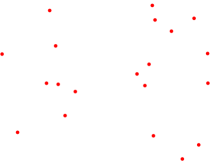
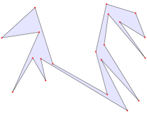
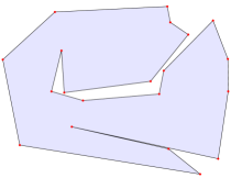
Figure 1. (Top) A set of 20 points. (Bottom Left) Min-Area solution. (Bottom Right) Max-Area solution.

1.1. Related Work

Most previous practical work has focused on finding heuristics for both problems. Taranilla et al. (Taranilla et al., 2011) proposed three different heuristics. Peethambaran (Peethambaran et al., 2015, 2016) later proposed randomized and greedy algorithms on solving Min-Area as well as the $d$-dimensional variant of both Min-Area and Max-Area. Considerable recent attention and progress was triggered by the 2019 CG Challenge, which asked contestants to find good solutions for a wide spectrum of benchmark instances with up to 100,000 points; details are described in the survey by Demaine et al. (Demaine et al., 2022).

Despite this focus, there has only been a limited amount of work on computing provably optimal solutions for instances of interesting size. The only notable exception is by Fekete et al. (Fekete et al., 2015), who were able to solve all instances of Min-Area with up to $n=14$ and some with up to $n=16$ points, as well as all instances of Max-Area with up to $n=17$ and some with up to $n=19$ points. This illustrates the inherent practical difficulty, which differs considerably from the closely related TSP, for which even straightforward IP-based approaches can yield provably optimal solutions for instances with hundreds of points, and sophisticated methods can solve instances with tens of thousands of points.

1.2. Our Results

We present a systematic study of exact methods for Min-Area and Max-Area polygonizations. We show that a number of careful enhancements can help to extend the range of instances that can be solved to provable optimality, with different approaches working better for the two problem variants. On the other hand, our work shows that the problems appear to be practically harder than geometric optimization problems such as the Euclidean TSP.

2. Context and Preliminaries

A detailed description of background, context and further connections can be found in the survey by Demaine et al. (Demaine et al., 2022).

3. Tools

We considered two models based on integer programming: an edge-based formulation (described in Section 3.1) and a triangle-based formulation (described in Section 3.2). In addition, we developed a number of further refinements and improvements (described in Section 3.3).

3.1. Edge-Based Formulation

The first formulation is based on considering directed edges of the polygon boundary. We denote the boundary of a polygon ${\mathcal{P}}$ by $\partial{{\mathcal{P}}}$. For two points $s_{i},s_{j}\in S$, we consider the two directed half-edges $e_{ij}$ and $e_{ji}$. Let $E^{r}$ be the set of half-edges between the points of $S$. As shown in Figure 2, the area $A_{{\mathcal{P}}}$ of a polygon ${\mathcal{P}}$ can be computed by adding the signed triangle areas $f_{e}$ that are formed by directed half-edges $e$ and an arbitrary, fixed reference point $r$: $f_{e}$ is positive if $e$ and $r$ form a triangle for which $e$ has a counterclockwise orientation along its boundary, and negative for a clockwise orientation. Therefore, we have to choose an appropriate set $E_{{\mathcal{P}}}\subseteq E^{r}$ that optimizes the total area, as follows.

(1) $$A_{{\mathcal{P}}}=A(E_{{\mathcal{P}}})=\sum_{e\in E_{{\mathcal{P}}}}f_{e}$$

(a) Triangles of the polygon.

(b) Positive edge triangles.

(c) Negative edge triangles.

(d) Calculated difference between (b) and (c)

Figure 2. Area calculation of a polygon using a reference point $r$ (red point)

This gives rise to an integer program in which the choice of half-edges $e=(i,j)$ is modeled by 0-1 variables $z_{e}=z_{ij}$.

(2) $$\{\min,\max\}\sum_{e\in E^{r}}z_{e}\cdot f_{e}\\$$

(3) $$\vphantom{\sum_{i=1}^{m}}\forall s_{i}\in S:\qquad \sum_{(j,i)\in\delta^{+}(s_{i})}z_{ji}=1$$

(4) $$\vphantom{\sum_{i=1}^{m}}\forall s_{i}\in S:\qquad \sum_{(i,j)\in\delta^{-}(s_{i})}z_{ij}=1$$

(5) $$\vphantom{\sum_{i=1}^{m}}\forall e=\{i,j\}\in E:\qquad z_{ij}+z_{ji}\leq 1$$

(6) $$\vphantom{\sum_{i=1}^{m}}\forall\text{intersecting}\quad\{i,j\},\{k,l\}\in E:\qquad z_{ij}+z_{ji}+z_{kl}+z_{lk}\leq 1$$

(9) $$\vphantom{\sum_{i=1}^{m}}(\forall\text{slabs}\quad L)(\forall m=1,\ldots,|L|):\qquad \sum_{i=1}^{m}z_{e_{i_{L}}^{lr}}-z_{e_{i_{L}}^{rl}}\begin{array}[]{l}\leq 1\\ \geq 0\end{array}$$

(12) $$\vphantom{\sum_{i=1}^{m}}\forall\emptyset\neq D\subsetneq S:\qquad \begin{array}[]{l}\sum_{(k,l)\in\delta^{-}(D)}z_{kl}\geq 1\\ \sum_{(k,l)\in\delta^{+}(D)}z_{kl}\geq 1\end{array}$$

(13) $$\forall{i,j}\in E:\qquad z_{ij},z_{ji}\in\{0,1\}$$

The objective function (2) arises from signed triangle areas, as described. The constraints (3) and (4) ensure that each point $s_{i}\in S$ has one outgoing edge and one incoming edge in the resulting polygon. Furthermore, constraints (5) guarantee, that for each possible edge, only one of the half-edges can be in $\partial P$. Intersecting edges in the resulting polygon are excluded by constraints (6).

Figure 3. Visualization of slabs in a polygon

Figure 4. Visualization of slab constraints. Left side shows a valid configuration. The right side shows a violated slab constraint.

The next set of inequalities (9) are called slab constraints; they ensure that the polygon is oriented in a counterclockwise manner. A slab $L$ is a vertical strip bounded by the $x$-coordinates of two consecutive points in the order of $x$-coordinates of points. Figure 3 shows the slabs of a given point set. The edges of slab $L$ get ordered by the $y$-coordinate at point $c_{L}=\frac{c^{x_{max}}_{L}-c^{x_{min}}_{L}}{2}$, where $c^{x_{max}}_{L}$ ($c^{x_{min}}_{L}$, resp.) is the $x$-coordinate of the right (left, resp.) boundary of slab $L$. Figure 3 illustrates $c_{L}$ with the blue arrow within the indicated slab. Now the bottommost chosen edge has to be oriented from left to right and the topmost one from right to left, while chosen edges in between have to alternate in their direction. This is enforced by the slab constraints for all possible sums $\sum_{i=1}^{m}z_{e_{i_{L}}^{lr}}-z_{e_{i_{L}}^{rl}}$ with $m=1,\dots,|L|$, where $e_{i_{L}}^{lr}$ ($e_{i_{L}}^{rl}$, resp.) denotes the $i$-th bottom most half-edge along slab $L$ going from left to right (from right to left, resp.). Figure 4 shows two possible configurations of a slab. The left one is a valid slab and satisfies all inequalities (9), while the right one does violate the constraint

$$\underbrace{e^{lr}_{1}-e_{1}^{rl}}_{=1}+\underbrace{e^{lr}_{2}-e_{2}^{rl}}_{=-1}+\underbrace{e^{lr}_{3}-e_{3}^{rl}}_{=0}+\underbrace{e^{lr}_{4}-e_{4}^{rl}}_{=0}+\underbrace{e^{lr}_{5}-e_{5}^{rl}}_{=-1}=-1\ngeq 0\quad m=5$$

Note that we have to add inequalities for all $m=1,\dotsc,|L|$. For the previous example all other inequalities are satisfied.

$$e^{lr}_{1}-e_{1}^{rl} =1\begin{array}[]{l}\geq 0\\ \leq 1\end{array}\quad m=1$$

$$e^{lr}_{1}-e_{1}^{rl} + e^{lr}_{2}-e_{2}^{rl} =0\begin{array}[]{l}\geq 0\\ \leq 1\end{array}\quad m=2$$

$$e^{lr}_{1}-e_{1}^{rl} + e^{lr}_{2}-e_{2}^{rl} + e^{lr}_{3}-e_{3}^{rl} =0\begin{array}[]{l}\geq 0\\ \leq 1\end{array}\quad m=3$$

$$e^{lr}_{1}-e_{1}^{rl} + e^{lr}_{2}-e_{2}^{rl} + e^{lr}_{3}-e_{3}^{rl} + e^{lr}_{4}-e_{4}^{rl} =0\begin{array}[]{l}\geq 0\\ \leq 1\end{array}\quad m=4$$

$$\underbrace{e^{lr}_{1}-e_{1}^{rl}}_{=1} + \underbrace{e^{lr}_{2}-e_{2}^{rl}}_{=-1} + \underbrace{e^{lr}_{3}-e_{3}^{rl}}_{=0} + \underbrace{e^{lr}_{4}-e_{4}^{rl}}_{=0} + \underbrace{e^{lr}_{5}-e_{5}^{rl}}_{=-1} + \underbrace{e^{lr}_{6}-e_{6}^{rl}}_{=1} =0\begin{array}[]{l}\geq 0\\ \leq 1\end{array}\quad m=6$$

The last set of constraints (12) are subtour constraints; they ensure that all non-trivial subsets of vertices have at least one incoming and one outgoing edge. These constraints are very common for many related optimization problems, including (in undirected form) for the TSP.

Overall, the size of the resulting IP is as follows.

• There is a total of $O(2n)=O(n)$ point degree constraints (3) and (4), two for each vertex.

• There is a total of $O(\binom{n}{2})=O(n^{2})$ half-edge constraints, one for each half-edge.

• There is a total of $O(n^{4})$ intersections constraints (6), one for each pair of intersecting edges.

• There is a total of $O(n^{3})$ slab constraints (9), one for each combination of one of the $n-1$ slabs and the $O(n^{2})$ possible edges crossing it.

• There is a total of $O(2^{n})$ subtour constraints (12), one for each non-trivial subset of vertices.

In the practical implementation we cannot add all subtour constraints and try to avoid adding intersection constraints before starting the branch and cut algorithm. While solving the IP we get access to partial solutions and only add new constraints when necessary. Therefore, we start with a slim IP with only $O(n+n^{2}+n^{3})=O(n^{3})$ constraints and $O(n^{2})$ variables. During the branch-and-cut algorithm at most $O(2^{n})$ constraints are added.

3.2. Triangle-Based Formulation

An alternative is the triangle-based formulation, which considers the set $T(P)$ of possibly $\binom{n}{3}$ many empty triangles of a point set $P$; see Figure 5 for an illustration. Making use of the fact that a simple polygon with $n$ vertices consists of $(n-2)$ empty triangles with non-intersection interiors, we get the following IP formulation, in which the presence of an empty triangle $\triangle$ with unsigned area $f_{\triangle}$ is described by a 0-1 variable $x_{\scaleto{\triangle}{5pt}}$.

Figure 5. A set of five points and its ten empty triangles.

(14) $$\{\min,\max\}\sum_{{\scaleto{\triangle}{5pt}}\in T(P)}f_{\scaleto{\triangle}{5pt}}\cdot x_{\scaleto{\triangle}{5pt}}\\$$

(15) $$\sum_{{\scaleto{\triangle}{5pt}}\in T}x_{\scaleto{\triangle}{5pt}}=n-2$$

(16) $$\vphantom{\sum_{i=1}^{n}}\forall s_{i}\in S:\qquad \sum_{{\scaleto{\triangle}{5pt}}\in\delta(s_{i})}x_{\scaleto{\triangle}{5pt}}\geq 1$$

(17) $$\vphantom{\sum_{i=1}^{m}}\forall\text{intersecting}\quad\triangle_{i},\triangle_{j}\in T(P):\qquad x_{{\scaleto{\triangle}{5pt}}_{i}}+x_{{\scaleto{\triangle}{5pt}}_{j}}\leq 1$$

(18) $$\vphantom{\sum_{i=1}^{n}}\forall\emptyset\neq D\subsetneq T(P),|D|\leq n-3:\qquad \sum_{{\scaleto{\triangle}{5pt}}\in D}x_{\scaleto{\triangle}{5pt}}-\sum_{{\scaleto{\triangle}{5pt}}\in\delta(D)}x_{\scaleto{\triangle}{5pt}}\leq|D|-1$$

(19) $$\vphantom{\sum_{i=1}^{n}}\forall\triangle\in T(P):\qquad x_{\scaleto{\triangle}{5pt}}\in\{0,1\}$$

The objective function (14) is the sum over the chosen triangles areas. Triangle constraint (15) ensures that we chose exactly $n-2$ triangles, which is the number of triangles in a triangulation of a simple polygon. Furthermore, point constraints (16) guarantee that a solution has at least one adjacent triangle at each point $s_{i}\in S$. Finally, intersection constraints (17) ensure that we only select triangles with disjoint interiors. As shown in Figure 6, these are indeed necessary, even when minimizing total area.

Figure 6. Triangulations of a point set with (right) and without (left) intersection constraints. The difference of both areas is the area difference of both red triangles.

Finally, the subtour constraints (18) ensure that the set of selected triangles forms a simple polygon: Either all triangles of $D$ are part of the solution and at least one new triangle must be adjacent to the boundary of $D$ (i.e., a triangle of $\delta(D)$), or one triangle of $D$ is not part of the solution (see Fig. 7 for a visualization).

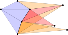
Figure 7. Visualization of the subtour constraint. Blue triangles represent the set $D$. To satisfy the subtour constraint, either one of the red or orange triangles must be added, or one of the blue triangles must be removed.

Overall, the size of the resulting IP is as follows.

• There is a single triangle constraint of type (15).

• There are $O(n)$ point constraints (16), one for each point $s_{i}\in S$.

• There are $O(n^{6})$ intersection constraints (17), one for each intersecting pair of the $O(n^{3})$ triangles.

• There are $O(2^{n^{3}})$ subtour constraints (18), one for each $D\subsetneq T$ with $0<|D|\leq n-3$ and all triangles in $D$.

Because of the enormous number of subtour constraints and the fact that most of the intersection constraints are not needed, both types are dynamically added during the branch-and-cut algorithm.

3.3. Enhancing the Integer Programs

Given the considerable size of the described IP formulations, we employed a number of enhancements to improve efficiency.

3.3.1. Convex Hull

The area of the convex hull is an upper bound for every polygonization of a given point set. Its combinatorial structure allows omitting a number of constraints: The edge $e$ between two non-adjacent points on the boundary of the convex hull divides the point set into two separate pieces, so we can remove edges between two non-adjacent points of the convex hull from our set of variables.

3.3.2. Initial Solutions

When solving an optimization problem, it helps to start with an initial integer solution, which leads to a polygon ${\mathcal{P}}_{initial}$. Until no better solution has been found, the area of ${\mathcal{P}}_{initial}$ helps the bounding process to cut off subtrees of possible solutions. Starting with a solution that is very close to the optimal solution can accelerate the computation speed a lot. As described in the survey article (Demaine et al., 2022), there is an approximation method by Fekete (Fekete, 1992) for the Max-Area problem, which guarantees to be at most $\frac{1}{2}$ as large as the optimal solution. For the minimization problem we use a heuristic without performance guarantee.

We also used a simple greedy approach to obtain an initial value for Min-Area, based on a heuristic of Taranilla et al. (Taranilla et al., 2011). The algorithm modifies an existing polygon ${\mathcal{P}}$ until all points are on the boundary.

1. Compute the convex hull of the point set $S$, resulting in the initial polygon ${\mathcal{P}}$.

2. Among all points inside ${\mathcal{P}}$ that are not part of ${\mathcal{P}}$, chose one point $s_{1}$. The point forms an empty triangle with some edge $\{s_{2},s_{3}\}$ of ${\mathcal{P}}$, does not intersect with $\partial{\mathcal{P}}$ and is maximum in size. If no point $s_{1}$ inside ${\mathcal{P}}$ exists, we are finished, because ${\mathcal{P}}$ is a simple polygon that has all points of $S$ on its boundary.

3. Remove edge $\{s_{2},s_{3}\}$ from ${\mathcal{P}}$ and add edges $\{s_{1},s_{2}\},\{s_{1},s_{3}\}$. Repeat Step 2.

Figure 8. A possible step two of the Greedy Min-Area algorithm

Figure 8 illustrates a possible second step of the Greedy Min-Area algorithm. The complexity of the first step is $O(n\log n)$, because we need to compute a convex hull. For the second step we need to consider each of the $n$ edges of ${\mathcal{P}}$ and compute triangles with possibly $n$ points inside ${\mathcal{P}}$. We need to check whether the triangle is empty and whether the triangle does not cross any of the $n$ edges of ${\mathcal{P}}$. The second step has to be carried out for every point that is not part of the convex hull, i.e., $n$ times. This leads to an overall complexity of $O(n^{4})$. The third step can be done in constant time $O(1)$. Overall, this leads to a complexity of of $O(n\log n+n^{4}+1)=O(n^{4})$ for Greedy Min-Area. If we take away triangles with minimum in step two of the algorithm, we get an heuristic for the maximization problem. We call this variant Greedy Max-Area.

3.3.3. Intersections

Intersection Cliques

If any pair $o_{i},o_{j}$ in a given set $C=\{o_{1},\ldots,o_{k}\}$ of objects (which may be edges or triangles) intersect, they form an intersection clique. Clearly, this allows replacing the $\Theta(k^{2})$ pairwise intersection constraints by a single one, as follows.

$$\sum_{i=1}^{k}x_{i}\leq 1.$$

Because of the NP-completeness of finding maximum cardinality cliques, we simply use maximal cliques.

We only add intersection constraints incrementally, i.e., whenever we get a new integer solution, we add new violated intersection constraints. Because it is very time-consuming to compute all maximal cliques in every iteration, we add cliques by consecutively adding more edges to an existing clique $C$ until no edge can be found, which intersects all edges in $C$. We start with $C=\{o_{1},o_{2}\}$ with $o_{1},o_{2}$ being two intersecting objects of the solution. We then try to add more objects of the current solution to the clique until no such object can be found. Afterwards all other objects are considered, until no object can be added to $C$. This provides good solutions in practice.

Halfspace Constraints

For the triangle-based approach, we introduce the concept of halfspace constraints. The goal is to reduce the number of intersections that need to be added during the optimization process by excluding obvious intersections from the beginning. Figure 9 shows the two types of intersections which may occur. Two intersecting triangles may share no point, a single point, or two points.

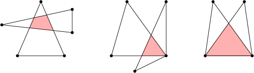
Figure 9. All three types of possible intersections in the triangle-based approach.

There are other intersections possible besides those in which two triangles share an edge. Two triangles $\triangle_{i},\triangle_{j}$ that share an edge $e$ intersect if both remaining points lie on the same side of $e$. Figure 10 illustrates this idea for three triangles. Points $s_{i},s_{j}\in S$ lie on the same side of $e$. Therefore, the triangles they form with $e$ do intersect. For points on the opposite site of $e$, such as $s_{k}$, the induced triangles with $e$ cannot intersect with those from $s_{i},s_{j}$.

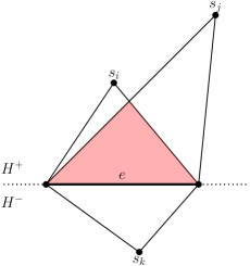
Figure 10. Intersections in the triangle-based approach with triangles sharing an edge

For every possible edge $e$ of the triangulation of the optimal polygon, at most one triangle may be on each side of the edge. We refer to $e$ as a hyperplane dividing the two-dimensional space into two halfspaces. Each halfspace may have one triangle $\triangle$ containing $e$. This allows us to formulate halfspace constraints, as follows.

(20) $$\forall e=\{s_{i},s_{j}\}\text{ with }s_{i}\neq s_{j}\land s_{i},s_{j}\in S:\begin{array}[]{l}\sum_{{\scaleto{\triangle}{5pt}}\in H^{+}(e)}x_{\scaleto{\triangle}{5pt}}\leq 1\\ \sum_{{\scaleto{\triangle}{5pt}}\in H^{-}(e)}x_{\scaleto{\triangle}{5pt}}\leq 1\end{array}$$

$H^{+}$ and $H^{-}$ are the two halfspaces induced by $e$ (see Figure 10). Because chords of the convex hull (CH-chords) cannot lie on the boundary of the polygonization, we can use the halfspace constraints to formulate a condition that applies to triangles that contain such edges. For these triangles, the sum over both halfspaces has to be the same to ensure that either the triangles are not part of the solution or if they are, there has to be a triangle on both sides of the edge.

(21) $$\forall\text{CH-chords }e:\sum_{{\scaleto{\triangle}{5pt}}\in H^{+}(e)}x_{\scaleto{\triangle}{5pt}}=\sum_{{\scaleto{\triangle}{5pt}}\in H^{-}(e)}x_{\scaleto{\triangle}{5pt}}$$

3.3.4. Branching on Variables

Another fine-tuning trick is based on a simple concept that makes use of the CPLEX callback API. As stated before, we may have not added all intersection constraints from the beginning. This leads to many interim solutions with intersecting edges.

Imagine a branching where two branches are created; subtree $T_{1}$ sets $x_{i}=1$ and $T_{0}$ sets $x_{i}=0$. We are interested in the branch $T_{1}$. In that subtree, $x_{i}$ is set to one. For all child nodes of $T_{1}$, object $o_{i}$ is part of the solution. Therefore, all intersecting object may not be set to one. In order to prevent the solver from unnecessary branching, we set all the intersecting entities to zero when branching on variable $x_{i}$. This leads to fewer intersection constraints and less branching in later stages.

For the triangle-based approach, we can make use of another characteristic. If we are certain that a group of triangles will not be part of a solution in the current branch, these triangles may be the last ones that are able to connect two unconnected components. In case we already branched variables of one component to one, we can exclude all variables of the other component. If we branched variables of both components to one, we can prune the current node, because there will be no future solution which connects both components.

3.3.5. Subtour Constraints

Both integer program formulations make use of the concept of subtour constraints. As described, these are only added incrementally during the optimization process.

Callback Graphs

The computation of subtours is problem specific in certain areas. However, if we abstract both problem’s interim solutions on undirected callback graphs $G$, the algorithmic approaches have multiple attributes in common. For the edge-based approach we create a vertex for each point $s_{i}\in S$ and connect those vertices $v_{i},v_{j}$, where $(i,j)$ or $(j,i)$ are part of the solution. In the triangle-base approach we build the dual graph, i.e., we have a vertex for each triangle of the solution, and an edge between adjacent triangles.

Connected Components

Finding violated subtour constraints in a given interim solution can simply be based on searching for connected components in the callback graph. For computing multiple connected component at once, we use a DFS-based approach that starts at a vertex $v_{i}$ and finds its connected component by iterating through the edges of the callback graph. If there is any non-visited vertex $v_{j}$, it repeats the last step until all vertices were visited. This method operates in time $O(n+|E|)$.

Edge-Based Approach

For a given interim solution we compute the connected components; for each such component $D$, we add one constraint over the sum of outgoing edges of $D$ and one constraint over the incoming edges of $D$.

$$\sum_{e\in\delta^{-}(D)}z_{e}\geq 1\qquad\sum_{e\in\delta^{+}(D)}z_{e}\geq 1$$

The constraints can be generated in $O(|E|)$, because we need to iterate over all edges to find out which one are leaving or entering the component. Figure 11 illustrates an example of three connected components in a solution. Observe that one of $\delta^{+}$ and one of $\delta^{-}$ edges has to be part of a correct solution in order to connect $D$ to the rest of the point set.

Figure 11. Three connected components of an interim solution

Triangle-Based Approach

For a given interim solution we compute the connected components. In contrast to the edge-based approach, we cannot find two sets $\delta^{+},\delta^{-}$, because the vertices of the callback graph do not have to be part of the optimal solution. This makes the problem of preventing subtours more complex, because each subtour constraint has to include an information about which vertices have been chosen so far. The main idea is to force a given component to have at least one neighbor included in the optimal solution. Iterating these constraints over the interim solutions will force two unconnected components to get connected.

Let $D$ be a connected set of triangles and let $\delta(D)$ be the set of all triangles having one edge on the outer boundary of $D$ and one point in $T\setminus D$.

(22) $$\sum_{{\scaleto{\triangle}{5pt}}\in D}x_{\scaleto{\triangle}{5pt}}\leq|D|-1+\sum_{{\scaleto{\triangle}{5pt}}\in\delta(D)}x_{\scaleto{\triangle}{5pt}}$$

Observe that the constraint forces a solution containing $D$ to attach at least one triangle to $D$. Note that the constraint is not as strong as the intersection constraint of the edge-based approach, because it depends on the configuration of $D$. The constraint is also satisfied if one triangle of $D$ gets exchanged by another.

Finding Minimum Cuts

If we consider fractional solutions of the Linear Programming relaxations of either problem, finding violated subtour constraints requires searching for minimum cuts. The simplest approach is to use one of the well-known max.flow algorithms. Ford and Fulkerson (Ford and Fulkerson, 1956) gave an elegant proof that a maximum flow $f$ is also a minimal cut in a flow network. For undirected graphs, Stoer and Wagner (Stoer and Wagner, 1997) provided an algorithm that finds a minimal cut in $O(|V|\cdot|E|+|V|^{2}\log|V|)$. To find more than one subtour, we can also search for min-cuts separating two given vertices $v_{i},v_{j}$. A minimum cut of $G$ will be one of the cuts separating two vertices $v_{i}\in V_{1}$ and $v_{j}\in V_{2}$. Gomory and Hu (Gomory and Hu, 1961) introduced the concept of edge-weighted Gomory-Hu-Trees $T(G)$. For every pair of vertices $v_{i},v_{j}\in V(G)$ the minimum cut separating $v_{i}$ and $v_{j}$ in $G$ is the minimum weighted edge of the path from $v_{i}$ to $v_{j}$ in $T(G)$. Using this technique we are able to add more than one subtour constraint at once.

3.4. Subtour Angle Constraints

For the next idea in the triangle-based approach we consider possible subtours.

Figure 12. Subtour types in the triangle-based approach: $C_{1}$ does not share a point with $C_{2}$ or $C_{3}$; $C_{2}$ and $C_{3}$ share the point $s_{i}$.

Figure 12 illustrates two different types of subtours that may occur in interim solutions of the triangle-based approach. The first type are connected components in the sense that two components $C_{i},C_{j}$ do not share a single point. In the illustration, $C_{1}$ and $C_{2}$ as well as $C_{1}$ and $C_{3}$ are components of such type. The second type are components that share one or more points. In Figure 12, this type is represented by the components $C_{2}$ and $C_{3}$ that share a point $s_{i}\in S$.

(a) Point connecting two components

(b) Possible solution closing the left side

(c) Possible solution closing the right side

Figure 13. Visualization of subtour angle constraints

The construction of the callback graph will detect both component types, as subtours and equations (22) would ensure later solutions that consist of one connected component. We consider two triangles that share a point $s_{i}$, but are not connected in the callback graph. If both triangles are part of the optimal solution, we can be sure that both triangles are connected with other triangles containing $s_{i}$. Let $t_{top},t_{bottom}$ be two triangles of different components sharing one point $s\in S$. Let $\alpha_{l},\alpha_{r}$ be the angles between the inner edges of $t_{top},t_{bottom}$ and $s$. Figure 13(a) illustrates both triangles and their respective angles. From now on we assume that both triangles are part of an optimal solution. Because an optimal solution has to be a valid polygon, both $t_{top}$ and $t_{bottom}$ have to be in the same component. The resulting polygon may not have both components only connected with triangles not including $s$. This leads to the fact that both components have to be connected via triangles in $\alpha_{l}$ or $\alpha_{r}$. Figures 13(b) and 13(c) show two possible cases of the optimal polygon, one closes $\alpha_{l}$, while the other one closes $\alpha_{r}$. The sum of inner angles at $s$ of these triangles has to be equal to $\alpha_{l}$ and $\alpha_{r}$ respectively.

$$\beta_{i}+\beta_{j}=\alpha_{l}\qquad\beta_{k}+\beta_{l}+\beta_{m}=\alpha_{r}$$

Note that no solution can have both angles filled completely, because $s$ would no longer be on the boundary of $P$. This leads to so-called subtour angle constraints. The main idea is that if both triangles $t_{top},t_{bottom}$ are part of the solution, other triangles at $s$ need to close at least an angle of $\min\{\alpha_{l},\alpha_{r}\}$.

(23) $$\min\{\alpha_{l},\alpha_{r}\}\cdot(z_{top}+z_{bottom}-1)\leq\sum_{{\scaleto{\triangle}{5pt}}\in\delta(s)}\beta_{{\scaleto{\triangle}{5pt}}}^{s}\cdot x_{\scaleto{\triangle}{5pt}}$$

By $\beta_{\scaleto{\triangle}{5pt}}^{s}$ we denote the inner angle of the triangle $\triangle$ at point $s$. Figures 13(b) and 13(c) illustrate how the angles $\beta_{\scaleto{\triangle}{5pt}}^{s}$ add up to $\alpha_{l/r}$. At every integer solution we obtain during the solving process, we have reason to believe that triangles of the integer solution have a high probability to be part of the optimal solution. Because of that, we add subtour angle constraints at every integer solution. In addition to the previous ideas, we generalize the idea of two triangles at one point to so-called triangle fans.

Definition 1.

In an interim solution a triangle fan is a set $F_{s}$ of connected triangles $\triangle$, which share a point $s\in S$. This means that there is a path $P$ for every $\triangle_{i},\triangle_{j}\in F_{s}$ in the callback graph.

Consider an interim solution obtained during the solving process. After constructing the callback graph, we iterate over all triangles of the solution and add each triangle to three triangle fans (one for each point of $\triangle$). The triangle $\triangle$ will be added to an existing fan $F_{s}$ if it is in the same component, because this indicates a path between $\triangle$ and the other $\triangle_{i}\in F_{s}$. If no such fan is found, a new fan will be created for this component. In the end we return all triangle fans for each point $s\in S$. Because a solution contains $n-2$ triangles, we will add at most $n-2$ triangles to their fan. As the triangle has three points, each triangle can be part of three fans. This leads to a time complexity of $O((n-2)\cdot 3\cdot(n-2))=O(n^{2})$ where $n$ is the number of points in $S$.

After computing all triangle fans we choose two triangles $t_{top},t_{bottom}$ with a common point $s$ from two different fans in order to formulate the constraint. These triangles should not be chosen at random, because the constraint gets much stronger if the following two conditions apply.

• The triangles should have a small area.

• The angles $\alpha_{l},\alpha_{r}$ are similar, i.e., they minimize $|\alpha_{l}-\alpha_{r}|$.

Consider two maximal fans $F_{1},F_{2}$ having a point $s$ in common. We choose triangles $t_{top}\in F_{1},t_{bottom}\in F_{2}$, such that $|\alpha_{l}-\alpha_{r}|$ is minimized. If there are multiple candidates, we choose those that minimize the area.

3.4.1. Point-based Subtour Constraints

Consider a point set $X\subseteq S$ of an interim solution with $3\leq|X|\leq n-2$. We denote $\dot{\triangle}\in\delta(X)$ and $\ddot{\triangle}\in\delta(X)$ to be triangles with exactly one corner or two corners inside $X$ respectively. We know that the point set $X$ has to be connected to at least two points outside of $X$. To connect both points to $X$, at least two triangles are needed that have at least one point outside of $X$ (see Fig. 14 right). This leads to the first point-based subtour constraint

(24) $$\sum_{\dot{\scaleto{\triangle}{5pt}}\in\delta(X)}x_{\dot{\scaleto{\triangle}{5pt}}}+\sum_{\ddot{\scaleto{\triangle}{5pt}}\in\delta(X)}x_{\ddot{\scaleto{\triangle}{5pt}}}\geq 2$$

Now suppose there is no triangle connecting two points from $X$. This implies that each point $s\in X$ needs a triangle connecting $s$ with two points from $S\setminus X$. Therefore, if $\sum_{\ddot{\scaleto{\triangle}{5pt}}\in\delta(X)}=0$, then $\sum_{\dot{\scaleto{\triangle}{5pt}}\in\delta(X)}x_{\dot{\scaleto{\triangle}{5pt}}}=|X|$ (see Fig. 14 left). If there is at least one triangle with two points in $X$, then a possible solution can exist with only one additional triangle. Thus, if $\sum_{\ddot{\scaleto{\triangle}{5pt}}\in\delta(X)}x_{\ddot{\scaleto{\triangle}{5pt}}}\geq 1$, then $\sum_{\dot{\scaleto{\triangle}{5pt}}\in\delta(X)}x_{\dot{\scaleto{\triangle}{5pt}}}+\sum_{\ddot{\scaleto{\triangle}{5pt}}\in\delta(X)}x_{\ddot{\scaleto{\triangle}{5pt}}}\geq 2$ (see Fig. 14 right). Combining both cases yields the following constraint for a point set $X$.

(25) $$\sum_{\dot{\scaleto{\triangle}{5pt}}\in\delta(X)}x_{\dot{\scaleto{\triangle}{5pt}}}\geq|X|-(|X|-1)\cdot\sum_{\ddot{\scaleto{\triangle}{5pt}}\in\delta(X)}x_{\ddot{\scaleto{\triangle}{5pt}}}$$

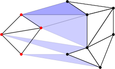
Figure 14. Illustration of point-based subtour constraints. Red points correspond to the set $X$. Left: A valid solution when no outgoing triangle (blue triangles) has two points from $X$. Then there must be $|X|$ triangles connecting $X$ to $S\setminus X$. Right: If at least one triangle has two points from $X$, then there must exist at least one more outgoing triangle.

Separation over these constraints can be achieved analogous to regular subtour constraints for the classic TSP, with triangles in our problem corresponding to vertices in the TSP, and connected components corresponding to connected sets of triangles. This allows polynomial-time separation, but requires iterating over the $O(n^{3})$ triangles.

4. Experiments

Based on the described approaches, we ran experiments on some machines with slightly different specifications and parameters. We used CPLEX 12.9 with a time limit of 1800 seconds on an AMD Ryzen 7 5800X CPU 4.2GHz with eight cores and 16 threads utilizing an L3 Cache with a size of 32MB. The solver was able to use a maximum amount of 128GB RAM. Our solver uses the default CPLEX parameters except CPXPARAM_Parallel, which was set to CPX_PARALLEL_OPPORTUNISTIC.

We considered all instances from the CG:SHOP Challenge with up to 50 points; see Section 4.3 for a detailed description. Because the original CG:SHOP benchmark set mostly aims at heuristic and experimental methods developed in the competition, it reaches all the way up to 1,000,000 points, but is relatively sparse within the range of exact methods. We accounted for this sparsity by generating additional instances of similar type; because of fast run times, we used 20 instances and 5 iterations each for instance sizes 12-20; for instance sizes 21-23, we considered 20 instances and 1 iteration each; for larger sizes, we limited the number to 10 instances each.

4.1. Solver Types

In this section we will introduce different versions for each solver that implement features that we mentioned in Section 3. For both the triangulation-based and edge-based approach, we pass a start solution that was generated by a Greedy Min-Area heuristic that is inspired by the work of Taranilla et al. (Taranilla et al., 2011), Fekete’s Max-Area approximation (Fekete, 1992) or solutions from the CG:SHOP competition. Greedy Min-Area starts with a polygon $P=conv(S)$ and carves out the largest triangles by replacing an edge $(p_{i},p_{j})$ of $P$ by two edges $(p_{i},q)(q,p_{j})$ to an inner point $q$.

4.1.1. Edge-Based Solvers

EdgeV1 is a basic integer program of the edge-based approach. It adds all intersection constraints and slab constraints before starting the solving process and adds subtour constraints in every integer solution. This integer program is an improvement to the edge-based MinArea integer program presented by Papenberg et al. (Papenberg, 2014; Fekete et al., 2015). In the former approach cycle based subtour constraints were added after an optimal solution has been found. This resulted in poor computing times even for small point sets. We also utilize properties of the convex hull to exclude certain variables, i.e., edges that connect two non-adjacent points on the convex hull, from the computation. EdgeV1 makes use of this concept by setting these variables to zero. EdgeV2 extends the previous version by adding intersection constraints at interim solutions. EdgeV3 includes a branching extension where branching on a variable $z_{e}$ results in intersecting edges getting branched to zero. In EdgeV4 we additionally search for subtours in fractional interim solutions and add slab constraints during the solving process. The upcoming sections will show that the edge-based approach is better suited for Max-Area instances.

4.1.2. Triangle-Based Solvers

TriangulationV1 is the first version of the triangle-based approach. Compared to the basic triangulation approach of Papenberg (Papenberg, 2014), we have fewer variables and different subtour constraints (18). We added further halfspace inequalities as well as equalities for edges which connect non-adjacent vertices of the convex hull. In TriangulationV1 we add subtour constraints and intersection constraints in every integer solution. TriangulationV2 extends the first version with so-called subtour angle constraints. These are added at every integer solution. We are able to reuse the connected components we need to compute along the way. This allows us to add constraints (18) without much additional computation time. TriangulationV3 makes use of additional results on ineffective subtour constraints. In addition to the constraints of TriangulationV2, we add point-based subtour constraints to every intermediate integer solution. The upcoming sections will show that the triangulation-based approach is better suited for Min-Area instances.

4.2. Analysis

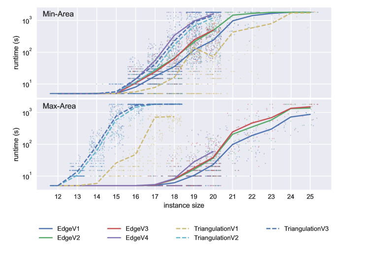
Figure 15. Runtimes for different solver versions on random instances of size $12-25$ and a time limit of $1800$ seconds. The line is the average runtime over five iterations on $20$ instances for sizes $12-20$. For sizes $21-25$ we solved one iteration on $20$ instances for sizes $21-23$ and $10$ instances of size $24-25$.

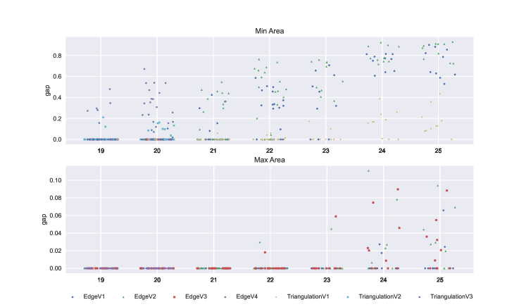
Figure 16. Optimality gap for instances with 19 to 25 points. Shown is the best gap over multiple runs for each instance.

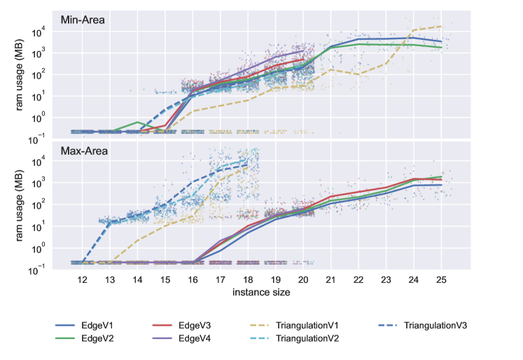
Figure 17. RAM usage for the experiments in Figure 15.

4.2.1. Edge-Based Solvers

We compared two different approaches. The first one, adds intersection constraints at every integer and at every fractional solution. The second one, adds intersection constraints at every integer solution. Our observations showed that searching for intersections in fractional solutions increases the computation time. We assume that the intersection constraints we obtain from fractional solutions are not needed for computing the optimal solution and that their generation wastes a lot of computation time. We denote EdgeV2 as the version which adds intersection constraints in every integer solution.

Figure 15 provides a detailed view on the runtime of the major Edge versions we consider in our experiments for instances of size $12-25$. The scatter plot shows the runtimes for different iterations and instances while the line is the average runtime over five iterations and $20$ instances for each $n\leq 20$. For $n>20$, we computed one iteration on $20$ instances (for sizes $21-23$) and $10$ instances (for sizes $24-25$). Figure 16 provides an overview over the optimality gap for instances with at least 19 points. Figure 17 illustrates the amount of memory that was used during the execution. As in other problems like TSP, adding constraints in interim solutions instead of adding all constraints in the beginning will only make significant impact when the instances reach a certain size. Our goal is to add fewer constraints in the beginning while preserving the baseline runtime and the high success rate of EdgeV1 for smaller instances. The best approach can then be used to solve larger instances where the construction of the complete integer program consumes too much space.

In comparison to the first version, EdgeV2 adds intersection constraints at every integer solution. Whenever many intersections constraints were needed to obtain the optimal solution, we observed that the runtime and the depth of the branch and bound tree increased. Figure 15 shows that the runtime for this approach was slightly higher than the EdgeV1 baseline. EdgeV3 further adds intersection constraints during branching, which preserved the low runtime on some instances while mitigating the negative effect on instances that needed a lot of intersection constraints. Apart from intersections one might want to add the slab constraints in interim solutions. Slab constraints ensure that the resulting polygon is oriented in the right direction. EdgeV4 adds slabs constraints during execution and searches for connected components, i.e. min-cuts in every fractional solution. We noticed that almost all of the slab constraints are added to the IP at some point during the execution of EdgeV4. As a consequence these constraints should be added from the beginning. In our implementation of EdgeV4, we computed the connected components of the interim solutions, i.e., minimum cuts with value one. We implemented multiple versions for finding minimum cuts of greater size. All approaches deteriorated the time needed for the computation. Moreover, the approach was unable to solve all instances of larger sizes within the time constraint. This shows that the computation of larger cuts is computationally expensive and the obtained inequalities not worth the effort.

Despite the low runtime on smaller instances, the number of unneeded intersection constraints added by EdgeV1 grows fast for larger instances. Therefore, the other approaches add fewer constraints, which results in better computation times. Overall the EdgeV2 approach which adds intersections in integral interim solutions or EdgeV3 which further uses some advanced branching techniques appear to be the best approaches for solving larger instances.

4.2.2. Triangle-Based Solver

As shown in Figure 17, the RAM usage of both approaches depend on the problem variant we are trying to solve. In Section 3.2 we proposed the triangle-based IP which uses $O(n^{3})$ variables and $O(n^{6})$ constraints (excluding subtour constraints). As a consequence, the formulation, branch and bound tree and temporary variables of the integer program require a lot of space on the executing machine. This is especially relevant for the Max-Area variant, for which many intersection constraints are needed to obtain a feasible solution.

Figure 15 provides a detailed view on the runtime of the major Triangle versions we considered in our experiments. Due to the triangulation approach performing worse on the Max-Area variant, we excluded instances of size $\geq 19$ in the experiment. The scatter plot shows the runtimes for different iterations and instances while the line is the average runtime over five iterations and $20$ instances for each $n\leq 20$. For $n>20$, we computed one iteration on $20$ instances (for sizes $21-23$) and $10$ instances (for sizes $24-25$).

As described above, there are only few intersections in interim solutions of the triangle-based approach when solving Min-Area instances, because overlapping areas are counterproductive for obtaining a minimal solution. Nevertheless, intersection constraints are possible and needed to be eliminated if no other constraints were found. The results of the edge-based approach showed that adding intersection clique constraints can be very efficient. We adapted the idea and searched for intersection cliques in TriangulationV1 as well. In TriangulationV2, we search for subtour angle constraints as well. Subtour angle constraints can help to decrease the runtime for some instances. In other occasions, the approach that added these constraints performed worse. We assume that better results can be achieved, if one improves the algorithm that finds the possible subtour constraints. We did not further investigate this opportunity as the triangulation approach has large space requirements for larger instances. Figure 17 shows that TriangulationV1 has a higher RAM usage than the edge-based approaches for $n\geq 24$. When attempting to solve the CG:SHOP instances to optimality in the next section, we reached the limit of $128GB$ for some instances of size $\geq 30$ and all instances of size $\geq 40$. The point based subtour constraints that were added in TriangulationV3 did not help to improve the performance of the approach and should not be considered as a valuable extension.

4.2.3. Convex Hull

During our experiments, we noticed a strong relation between the number of points on the convex hull in an instance and the runtime that is needed to find an optimal solution. We therefore generated instances with $n$ points and $3\leq k\leq n$ points on the convex hull. This was done by first generating $k$ points in convex position, taking points uniformly at random, discarding all points that would either lie in the interior or cause some previously selected points to lie in the interior. We then added $n-k$ points within the convex hull chosen uniformly at random.

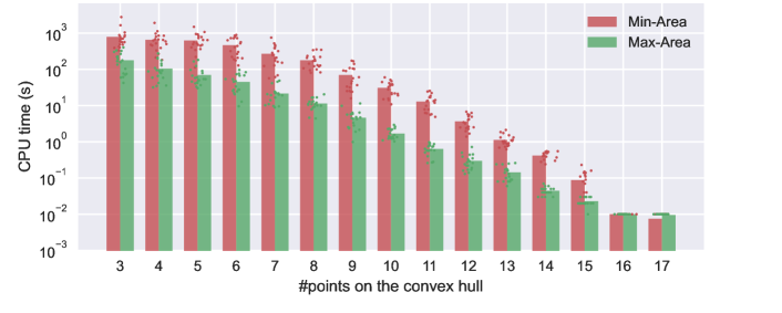
Figure 18. Runtime for the solver EdgeV1 with $n=17$ points and $20$ instances with a convex hull size of $k$ for every $k=3,\dots,17$.

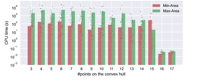
Figure 19. Runtime for the solver TriangulationV1 with $n=17$ points and $20$ instances with a convex hull size of $k$ for every $k=3,\dots,17$.

We performed an experiment for the solver EdgeV1 with $n=17$ points and generated $20$ instances for every $k=3,\dots,17$. Figure 18 compares the average aggregated CPU times, that is, the sum of time used by all processors during the optimization phase. We can clearly observe that the CPU time drastically decreases when more points lie on the convex hull of a point set. We assume that this is due to the fact that fewer edges are possible candidates and the number of possible polygonizations is smaller for these instances. Moreover, edges that connect two non-adjacent points of $conv(S)$ are set to zero, simplifying many constraints of the IP. On the other hand, Figure 19 shows the average CPU times for the triangulation approach TriangulationV1. Apart from a drastic decrease at $k=16,17$, we could only observe a minor trend towards shorter runtimes for larger $k$.

4.3. CG:SHOP Results

In this section, we discuss the results both IPs obtained on the CG:SHOP competition instances. We start off with small instances that the approaches were able to solve optimally in short time. Table 1 shows the runtimes for the smallest instances of the competition.

instance	size	Min-Area	runtime (s)	Max-Area	runtime (s)
uniform-0000010-1	10	58872	0.10000	148010	0.02000
uniform-0000010-2	10	51568	0.03000	151540	0.03000
london-0000010	10	19207298	0.09000	95364394	0.04000
euro-night-0000010	10	9954272	0.06000	28498980	0.04000
us-night-0000010	10	3650560	0.10000	13059816	0.08000
stars-0000010	10	40264246222	0.40000	127476507282	0.02000
uniform-0000015-1	15	102716	14.03000	391474	0.58000
uniform-0000015-2	15	113436	3.77000	374516	0.35000
london-0000015	15	17809096	5.07000	127729316	0.38000
euro-night-0000015	15	7107334	19.49000	37961104	2.03000
us-night-0000015	15	16642190	29.90000	60295830	4.49000
stars-0000015	15	29776831822	13.28000	142470465062	0.92000

Table 1. CG:SHOP results for Min-Area and Max-Area for instances of size $<20$.

As point sizes $\leq 15$ have been observed to be solvable by both approaches in a very short time period (see Section 4.2), we only show results from the Edge approach. In comparison with the Min-Area runtimes on uniformly distributed random instances in Figure 15, the runtimes on the competition instances appear to be similar. Note that the runtimes in the table are the best runtimes, we observed on these instances instead of the average runtime.

As explained earlier, the space requirements for the triangulation approach prevents experiments with larger instance sizes. Results from Section 4.2 imply that the edge-based approach is better suited for the Max-Area variant. In this paragraph, we investigate the results that were obtained on instances of size $20-50$ from the competition. For larger instances, we raised the maximum runtime to $43,800$ seconds because it is very unlikely to find an optimal solution especially for the larger instances. As other competitors submitted their best solutions on the same instances, we were able to provide the IP with these solutions, i.e. the best solution that was found during the competition. As most solutions are most likely the optimal solution of the corresponding instance, the main objective was to find good bounds within the time constraint. Keep in mind that we only present the best results that we obtained after numerous attempts on solving the instances.

Table 2. CG:SHOP results for Max-Area (edge-based) for instances of size $20-50$

instance	solver	size	competition	IP	best bound	gap	gap (convex hull)	runtime (s)
euro-night-0000020	E	20	43453166	43453166	43453166	0	0.09910	64.24
london-0000020	E	20	200514948	200514948	200514948	0	0.11300	124.84
stars-0000020	E	20	216742984910	216742984910	216742984910	0	0.05630	16.91
uniform-0000020-1	E	20	761968	761968	761968	0	0.15700	100.63
uniform-0000020-2	E	20	804730	804730	804730	0	0.08490	16.85
us-night-0000020	E	20	54561746	54561746	54561746	0	0.06340	13.04
euro-night-0000025	E	25	50782240	50782240	50782240	0	0.10170	15925.92
london-0000025	E	25	231544442	231544442	231544442	0	0.06950	2321.83
stars-0000025	E	25	237309787430	237309787430	237309787430	0	0.07350	6398.03
uniform-0000025-1	E	25	1320082	1320082	1320082	0	0.19820	26839.26
uniform-0000025-2	E	25	1379588	1379588	1379588	0	0.12530	1354.81
us-night-0000025	E	25	60585868	60585868	60585868	0	0.08360	1380.2074
euro-night-0000030	E	30	52830622	52830622	56079768	0.06150	0.08350	-
london-0000030	E	30	151703726	151703726	161269214.27440	0.06310	0.09240	-
stars-0000030	E	30	185057287956	185057287956	197980842032	0.06980	0.08390	-
uniform-0000030-1	E	30	1956068	1956068	2067442.99220	0.05690	0.08680	-
uniform-0000030-2	E	30	2309760	2309760	2402044.10610	0.04000	0.07960	-
us-night-0000030	E	30	66217320	66217320	70264245.99140	0.06110	0.07540	-
euro-night-0000035	E	35	45819094	45819094	48532070.61540	0.05920	0.07490	-
london-0000035	E	35	215109002	215109002	215109002	0	0.08270	100.4485
stars-0000035	E	35	222429730998	222429730998	239177631315	0.07530	0.09420	-
uniform-0000035-1	E	35	3234656	3234656	3467516.96170	0.07200	0.08160	-
uniform-0000035-2	E	35	3255396	3255396	3494212.54550	0.07340	0.08450	-
us-night-0000035	E	35	77135624	77135624	82463136	0.06910	0.08810	-
euro-night-0000040	E	40	47910104	47910104	50634608.01820	0.05690	0.05970	-
london-0000040	E	40	209674650	209674650	209674650	0	0.13340	3948.63
stars-0000040	E	40	190177150422	190177150422	207054663704.00031	0.08870	0.11460	-
uniform-0000040-1	E	40	4431360	4431360	4822510	0.08830	0.09010	-
uniform-0000040-2	E	40	4170194	4170194	4506200	0.08060	0.09100	-
us-night-0000040	E	40	68940956	68940956	72625076.83330	0.05340	0.05800	-
euro-night-0000045	E	45	48214668	48214668	48214668	0	0.07190	3267.89
london-0000045	E	45	271205760	271205760	292963145.99330	0.08020	0.09140	-
stars-0000045	E	45	245048373286	245048373286	266232485329.99460	0.08640	0.08640	-
uniform-0000045-1	E	45	4759374	4759374	5231150	0.09910	0.09910	-
uniform-0000045-2	E	45	5158094	5158094	5682168	0.10160	0.10160	-
us-night-0000045	E	45	77941112	77941112	77941112	0	0.02900	292.6256
euro-night-0000050	E	50	60399328	60399328	65414966	0.08300	0.24920	-
london-0000050	E	50	231089684	231089684	250510480	0.08400	0.08640	-
stars-0000050	E	50	247712484090	247712484090	264902562115.99869	0.06940	0.06940	-
uniform-0000050-1	E	50	6385168	6385168	6899665.99120	0.08060	0.08060	-
uniform-0000050-2	E	50	7151224	7151224	7848421.98230	0.09750	0.09750	-
us-night-0000050	E	50	79952918	79952918	80759104	0.01010	0.04040	-

Table LABEL:tab:cgshop-gaps shows the gap between the best solution and the best bound that was found by CPLEX. In accordance with CPLEX, we use $gap(obj,b)=\frac{|b-obj|}{10^{-10}+|obj|}$ for calculating the gap, where $b$ is the best bound and $obj$ is the objective function value of the best integer solution. The table also includes the gap to the size of the convex hull for comparison. The edge-based approach was able to prove optimality for all instances of size $\leq 25$. Most gaps between the convex hull and the best integer solution are below $0.10$ for larger instances. Despite the absolute differences, which are not accounted for by the specified bounds, the relative differences are quite small. The largest instance that was proven to be optimal was the euro-night-000045 instance, which contains $45$ points. To the best of our knowledge, this is the largest Max-Area instance that was solved to provable optimality. For instance sizes $>45$ we could not observe much improvement in the upper bounds in comparison to the trivial bound. One needs to add better cuts during the solving process to gather better bounds for these sizes.

Table 3. CG:SHOP results for Min-Area (both approaches) for instances of size $20-50$

instance	solver	size	competition	IP	best bound	gap	runtime (s)
euro-night-0000020	T	20	6703352	6703352	6703352	0	5.0056
london-0000020	T	20	40978058	40978058	40978058	0	5.0056
stars-0000020	T	20	41041275182	41041275182	41041275182	0	13.29
uniform-0000020-1	T	20	188242	188242	188242	0	25.0389
uniform-0000020-2	T	20	130478	130478	130478	0	5.8
us-night-0000020	T	20	6615280	6615280	6615280	0	4.03
euro-night-0000025	T	25	6235066	6235066	6235066	0	1954.56
london-0000025	T	25	31936238	31936238	31936238	0	37.03
stars-0000025	T	25	35893175226	35893175226	35893175226	0	582.5526
uniform-0000025-1	T	25	319974	319974	307238.12120	0.03980	-
uniform-0000025-2	T	25	351446	351446	351446	0	845.3083
us-night-0000025	T	25	9123288	9123288	9123288	0	73.08
euro-night-0000030	T	30	7190308	7190308	3896089.33430	0.45810	-
london-0000030	T	30	15533240	15533240	9782667.47350	0.37020	-
stars-0000030	T	30	28318464852	28318464852	18121788612.62220	0.36010	-
uniform-0000030-1	T	30	373510	373510	353361	0.05390	-
uniform-0000030-2	T	30	427002	427002	283974.11740	0.33500	-
us-night-0000030	T	30	5750296	5750296	3965540.66670	0.31040	-
euro-night-0000035	T	35	5470084	5470084	3040936.87770	0.44410	-
london-0000035	E	35	25363958	25363958	25363958	0	544.42
stars-0000035	T	35	33183160522	33183160522	17014719428.44230	0.48720	-
uniform-0000035-1	T	35	499776	499776	238522.74400	0.52270	-
uniform-0000035-2	T	35	430856	430856	269129.42060	0.37540	-
us-night-0000035	T	35	10123092	10123092	4883885.67640	0.51760	-
euro-night-0000040	E	40	4423466	4423466	4423466	0	694.9955
london-0000040	E	40	35905290	35905290	1	1	-
stars-0000040	E	40	34302635012	34302635012	1	1	-
uniform-0000040-1	E	40	777956	777956	18319.05880	0.97650	-
uniform-0000040-2	E	40	626084	626084	1	1	-
us-night-0000040	E	40	5267414	5267414	1	1	-
euro-night-0000045	E	45	5712456	5712456	1	1	-
london-0000045	E	45	33322976	33322976	33322976	0	39849.8
stars-0000045	E	45	31524828442	31524828442	1	1	-
uniform-0000045-1	E	45	813802	813802	1	1	-
uniform-0000045-2	E	45	741648	741648	1	1	-
us-night-0000045	E	45	3595152	3595152	95814	0.97330	-
euro-night-0000050	E	50	7204726	7204726	1	1	-
london-0000050	E	50	31064970	31064970	1	1	-
stars-0000050	E	50	26625487604	26625487604	26625487604	0	7796.55
uniform-0000050-1	E	50	625044	625044	1	1	-
uniform-0000050-2	E	50	1094266	1094266	1094266	0	7903.57
us-night-0000050	E	50	5054470	5054470	1	1	-

For the edge-based approach the minimization variant is significantly harder than the Max-Area problem for most instances. Unfortunately, the triangulation-based approach consumes a lot of space on larger point sets. Table LABEL:tab:cgshop-gaps-min summarizes our results on Min-Area. For instances of size $20-35$ (except london-0000035), the best results could be obtained using TriangulationV1. For the other instances the space requirements were too high and thus the edge-based approach was used. Apart from the instance uniform-0000025-1 all instances of size $20-25$ could be solved to optimality. For most of the larger instances of size $>35$, the edge-based approach was unable to improve the trivial bound of 1 (all solutions in the competition must have integral area). However, the competition results for the instances london-0000045, uniform-0000050-2 and stars-0000050 were proven to be optimal. To the best of our knowledge uniform-0000050-2 and stars-0000050 are the largest Min-Area instances that could be solved optimally. For instance size $>50$ we did not observe any improvement in the bounds. Apart from the optimal solutions, the edge-based approach is not well-suited for the minimization variant. Other approaches or improvements to the triangulation-based IP will most likely help to find better bounds.

5. Conclusions

While our work shows that with some amount of algorithm engineering, it is possible to extend the range of instances that can be solved to provable optimality, it also illustrates the practical difficulty of the problem. This reflects the limitations of such IP-based methods: The edge-based approach makes use of an asymmetric variant of the TSP, which is known to be harder than the symmetric TSP, while the triangle-based approach suffers from its inherently large number of variable and constraints. Furthermore, the non-local nature of Min-Area and Max-Area polygons (which may contain edges that connect far-away points) makes it difficult to reduce the set of candidate edges.

As a result, Min-Area and Max-Area turn out to be prototypes of geometric optimization problems that are difficult both in theory and practice. This differs fundamentally from a problem such as Minimum Weight Triangulation, for which provably optimal solutions to huge point sets can be found (Haas, 2018), and practically difficult instances seem elusive (Fekete et al., 2020)

References

- (1)
- Demaine et al. (2022) Erik D. Demaine, Sándor P. Fekete, Phillip Keldenich, Dominik Krupke, and Joseph S.B. Mitchell. 2022. Area-Optimal Polygonalizations: The 2019 CG Challenge. Journal of Experimental Algorithms (2022). To appear.
- Fekete (1992) Sándor P. Fekete. 1992. Geometry and the Travelling Salesman Problem. Ph.D. Thesis. Department of Combinatorics and Optimization, University of Waterloo, Waterloo, ON.
- Fekete (2000) Sándor P. Fekete. 2000. On simple polygonizations with optimal area. Discrete & Computational Geometry 23, 1 (2000), 73–110.
- Fekete et al. (2015) Sándor P. Fekete, Stephan Friedrichs, Michael Hemmer, Melanie Papenberg, Arne Schmidt, and Julian Troegel. 2015. Area-and boundary-optimal polygonalization of planar point sets. In European Workshop on Computational Geometry (EuroCG). 133–136.
- Fekete et al. (2020) Sándor P. Fekete, Andreas Haas, Dominik Krupke, Yannic Lieder, Eike Niehs, Michael Perk, Victoria Sack, and Christian Scheffer. 2020. Hard Instances of the Minimum-Weight Triangulation Problem. In European Workshop on Computational Geometry (EuroCG). 29:1–29:9.
- Fekete and Pulleyblank (1993) Sándor P. Fekete and William R. Pulleyblank. 1993. Area optimization of simple polygons. In Proc. 9th Symposium on Computational Geometry (SoCG). 173–182.
- Ford and Fulkerson (1956) Lester R Ford and Delbert R Fulkerson. 1956. Maximal flow through a network. Canadian journal of Mathematics 8, 3 (1956), 399–404.
- Gomory and Hu (1961) Ralph E Gomory and Tien Chung Hu. 1961. Multi-terminal network flows. J. Soc. Indust. Appl. Math. 9, 4 (1961), 551–570.
- Haas (2018) Andreas Haas. 2018. Solving Large-Scale Minimum-Weight Triangulation Instances to Provable Optimality. In Symposium on Computational Geometry (SoCG). 44:1–44:14.
- Papenberg (2014) Melanie Papenberg. 2014. Exact methods for area-optimal polygons. Master’s thesis. Braunschweig University of Technology.
- Peethambaran et al. (2015) Jiju Peethambaran, Amal Dev Parakkat, and Ramanathan Muthuganapathy. 2015. A randomized approach to volume constrained polyhedronization problem. Journal of Computing and Information Science in Engineering 15, 1 (2015), 011009.
- Peethambaran et al. (2016) Jiju Peethambaran, Amal Dev Parakkat, and Ramanathan Muthuganapathy. 2016. An Empirical Study on Randomized Optimal Area Polygonization of Planar Point Sets. Journal of Experimental Algorithmics 21 (2016), 1–10.
- Stoer and Wagner (1997) Mechthild Stoer and Frank Wagner. 1997. A simple min-cut algorithm. Journal of the ACM (JACM) 44, 4 (1997), 585–591.
- Taranilla et al. (2011) Maria Teresa Taranilla, Edilma Olinda Gagliardi, and Gregorio Hernández Peñalver. 2011. Approaching minimum area polygonization. In Congreso Argentino de Ciencias de la Computación (CACIC). 161–170.