Stateful Dynamic Partial Order Reduction for Model Checking Event-Driven Applications that Do Not Terminate

Abstract

Event-driven architectures are broadly used for systems that must respond to events in the real world. Event-driven applications are prone to concurrency bugs that involve subtle errors in reasoning about the ordering of events. Unfortunately, there are several challenges in using existing model-checking techniques on these systems. Event-driven applications often loop indefinitely and thus pose a challenge for stateless model checking techniques. On the other hand, deploying purely stateful model checking can explore large sets of equivalent executions.

In this work, we explore a new technique that combines dynamic partial order reduction with stateful model checking to support non-terminating applications. Our work is (1) the first dynamic partial order reduction algorithm for stateful model checking that is sound for non-terminating applications and (2) the first dynamic partial reduction algorithm for stateful model checking of event-driven applications. We experimented with the IoTCheck dataset—a study of interactions in smart home app pairs. This dataset consists of app pairs originated from 198 real-world smart home apps. Overall, our DPOR algorithm successfully reduced the search space for the app pairs, enabling 69 pairs of apps that did not finish without DPOR to finish and providing a 7$\times$ average speedup.

1 Introduction

Event-driven architectures are broadly used to build systems that react to events in the real world. They include smart home systems, GUIs, mobile applications, and servers. For example, in the context of smart home systems, event-driven systems include Samsung SmartThings [46], Android Things [16], Openhab [35], and If This Then That (IFTTT) [21].

Event-driven architectures can have analogs of the concurrency bugs that are known to be problematic in multithreaded programming. Subtle programming errors involving the ordering of events can easily cause event-driven programs to fail. These failures can be challenging to find during testing as exposing these failures may require a specific set of events to occur in a specific order. Model-checking tools can be helpful for finding subtle concurrency bugs or understanding complex interactions between different applications [49]. In recent years, significant work has been expended on developing model checkers for multithreaded concurrency [2, 19, 22, 25, 63, 61, 56, 59], but event-driven systems have received much less attention [22, 30].

Event-driven systems pose several challenges for existing stateless and stateful model-checking tools. Stateless model checking of concurrent applications explores all execution schedules without checking whether these schedules visit the same program states. Stateless model checking often uses dynamic partial order reduction (DPOR) to eliminate equivalent schedules. While there has been much work on DPOR for stateless model checking of multithreaded programs [12, 2, 25, 63, 19], stateless model checking requires that the program under test terminates for fair schedules. Event-driven systems are often intended to run continuously and may not terminate. To handle non-termination, stateless model checkers require hacks such as bounding the length of executions to verify event-driven systems.

Stateful model checking keeps track of an application’s states and avoids revisiting the same application states. It is less common for stateful model checkers to use dynamic partial order reduction to eliminate equivalent executions. Researchers have done much work on stateful model checking [55, 18, 32, 17]. While stateful model checking can handle non-terminating programs, they miss an opportunity to efficiently reason about conflicting transitions to scale to large programs. In particular, typical event-driven programs such as smart home applications have several event handlers that are completely independent of each other. Stateful model checking enumerates different orderings of these event handlers, overlooking the fact that these handlers are independent of each other and hence the orderings are equivalent.

Stateful model checking and dynamic partial order reduction discover different types of redundancy, and therefore it is beneficial to combine them to further improve model-checking scalability and efficiency. For example, we have observed that some smart home systems have several independent event handlers in our experiments, and stateful model checkers can waste an enormous amount of time exploring different orderings of these independent transitions. DPOR can substantially reduce the number of states and transitions that must be explored. Although work has been done to combine DPOR algorithms with stateful model checking [60, 62] in the context of multithreaded programs, this line of work requires that the application has an acyclic state space, i.e., it terminates under all schedules. In particular, the approach of Yang et al. [60] is designed explicitly for programs with acyclic state space and thus cannot check programs that do not terminate. Yi et al. [62] presents a DPOR algorithm for stateful model checking, which is, however, incorrect for cyclic state spaces. For instance, their algorithm fails to produce the asserting execution in the example we will discuss shortly in Figure 1. As a result, prior DPOR techniques all fall short for checking event-driven programs such as smart home apps, that, in general, do not terminate.

Our Contributions. In this work, we present a stateful model checking technique for event-driven programs that may not terminate. Such programs have cyclic state spaces, and existing algorithms can prematurely terminate an execution and thus fail to set the necessary backtracking points to fully explore a program’s state space. Our first technical contribution is the formulation of a sufficient condition to complete an execution of the application that ensures that our algorithm fully explores the application’s state space.

In addition to the early termination issue, for programs with cyclic state spaces, a model checker can discover multiple paths to a state $s$ before it explores the entire state space that is reachable from state $s$. In this case, the backtracking algorithms used by traditional DPOR techniques including Yang et al. [60] can fail to set the necessary backtracking points. Our second technical contribution is a graph-traversal-based algorithm to appropriately set backtracking points on all paths that can reach the current state.

Prior work on stateful DPOR only considers the multithreaded case and assumes algorithms know the effects of the next transitions of all threads before setting backtracking points. For multithreaded programs, this assumption is not a serious limitation as transitions model low-level memory operations (i.e., reads, writes, and RMW operations), and each transition involves a single memory operation. However, in the context of event-driven programs, events can involve many memory operations that access multiple memory locations, and knowing the effects of a transition requires actually executing the event. While it is conceptually possible to execute events and then rollback to discover their effects, this approach is likely to incur large overheads as model checkers need to know the effects of enabled events at each program state. As our third contribution, our algorithm avoids this extra rollback overhead by waiting until an event is actually executed to set backtracking points and incorporates a modified backtracking algorithm to appropriately handle events.

We have implemented the proposed algorithm in the Java Pathfinder model checker [55] and evaluated it on hundreds of real-world smart home apps. We have made our DPOR implementation publicly available [50].

Paper Structure. The remainder of this paper is structured as follows: Section 2 presents the event-driven concurrency model that we use in this work. Section 3 presents the definitions we use to describe our stateful DPOR algorithm. Section 4 presents problems when using the classic DPOR algorithm to model check event-driven programs and the basic ideas behind how our algorithm solves these problems. Section 5 presents our stateful DPOR algorithm for event-driven programs. Section 6 presents the evaluation of our algorithm implementation on hundreds of smart home apps. Section 7 presents the related work; we conclude in Section 8.

2 Event-Driven Concurrency Model

In this section, we first present the concurrency model of our event-driven system and then discuss the key elements of this system formulated as an event-driven concurrency model. Our event-driven system is inspired by—and distilled from—smart home IoT devices and applications deployed widely in the real world. Modern smart home platforms support developers writing apps that implement useful functionality on smart devices. Significant efforts have been made to create integration platforms such as Android Things from Google [16], SmartThings from Samsung [46], and the open-source openHAB platform [35]. All of these platforms allow users to create smart home apps that integrate multiple devices and perform complex routines, such as implementing a home security system.

The presence of multiple apps that can control the same device creates undesirable interactions [49]. For example, a homeowner may install the FireCO2Alarm [38] app, which upon the detection of smoke, sounds alarms and unlocks the door. The same homeowner may also install the Lock-It-When-I-Leave [1] app to lock the door automatically when the homeowner leaves the house. However, these apps can interact in surprising ways when installed together. For instance, if smoke is detected, FireCO2Alarm will unlock the door. If someone leaves home, the Lock-It-When-I-Leave app will lock the door. This defeats the intended purpose of the FireCO2Alarm app. Due to the increasing popularity of IoT devices, understanding and finding such conflicting interactions has become a hot research topic [27, 28, 54, 53, 57] in the past few years. Among the many techniques developed, model checking is a popular one [58, 49]. However, existing DPOR-based model checking algorithms do not support non-terminating event-handling logic (detailed in Section 4), which strongly motivates the need of developing new algorithms that are both sound and efficient in handling real-world event-based (e.g., IoT) programs.

2.1 Event-Driven Concurrency Model

We next present our event-driven concurrency model (see an example of event-driven systems in Appendix 0.A). We assume that the event-driven system has a finite set $\mathcal{E}$ of different event types. Each event type $\hbox{$e$}\in\hbox{$\mathcal{E}$}$ has a corresponding event handler that is executed when an instance of the event occurs. We assume that there is a potentially shared state and that event handlers have arbitrary access to read and write from this shared state.

An event handler can be an arbitrarily long finite sequence of instructions and can include an arbitrary number of accesses to shared state. We assume event-handlers are executed atomically by the event-driven runtime system. Events can be enabled by both external sources (e.g., events in the physical world) or event handlers. Events can also be disabled by the execution of an event handler. We assume that the runtime system maintains an unordered set of enabled events to execute. It contains an event dispatch loop that selects an arbitrary enabled event to execute next.

This work is inspired by smart-home systems that are widely deployed in the real world. However, the proposed techniques are general enough to handle other types of event-driven systems, such as web applications, as long as the systems follow the concurrency model stated above.

2.2 Background on Stateless DPOR

Partial order reduction is based on the observation that traces of concurrent systems are equivalent if they only reorder independent operations. These equivalence classes are called Mazurkiewicz traces [31]. The classical DPOR algorithm [12] dynamically computes persistent sets for multithreaded programs and is guaranteed to explore at least one interleaving in each equivalence class.

The key idea behind the DPOR algorithm is to compute the next pending memory operation for each thread, and at each point in the execution to compute the most recent conflict for each thread’s next operation. These conflicts are used to set backtracking points so that future executions will reverse the order of conflicting operations and explore an execution in a different equivalence class. Due to space constraints, we refer the interested readers to [12] for a detailed description of the original DPOR algorithm.

3 Preliminaries

We next introduce the notations and definitions we use throughout this paper.

Transition System. We consider a transition system that consists of a finite set $\mathcal{E}$ of events. Each event $\hbox{$e$}\in\hbox{$\mathcal{E}$}$ executes a sequence of instructions that change the global state of the system.

States. Let States be the set of the states of the system, where $\hbox{$s_{0}$}\in\hbox{$\textit{States}$}{}$ is the initial state. A state $s$ captures the heap of a running program and the values of global variables.

Transitions and Transition Sequences. Let $\mathcal{T}$  be the set of all transitions for the system. Each transition $\hbox{$t$}\in\hbox{$\mathcal{T}$}\>$ is a partial function from States to States. The notation $\hbox{$t_{s,e}$}=\textit{next}\left(\hbox{$s$},\hbox{$e$}\right)$ returns the transition $t_{s,e}$ from executing event $e$ on program state $s$. We assume that the transition system is deterministic, and thus the destination state $\hbox{\emph{dst}}{}(\hbox{$t_{s,e}$})$ is unique for a given state $s$ and event $e$. If the execution of transition $t$ from $s$ produces state $\hbox{$s$}^{\prime}$, then we write $\hbox{$s$}\xrightarrow{\hbox{$t$}}\hbox{$s$}^{\prime}$.

We formalize the behavior of the system as a transition system $\hbox{$A_{G}$}=(\hbox{$\textit{States}$}{},\Delta,\hbox{$s_{0}$})$, where $\Delta\subseteq\hbox{$\textit{States}$}{}\times\hbox{$\textit{States}$}{}$ is the transition relation defined by

$$(\hbox{$s$},\hbox{$s$}^{\prime})\in\Delta\>\>\text{iff}\>\>\exists\hbox{$t$}\in\hbox{$\mathcal{T}$}:\hbox{$s$}\xrightarrow[]{\hbox{$t$}}\hbox{$s$}^{\prime}$$

and $s_{0}$ is the initial state of the system.

A transition sequence $\mathcal{S}$ of the transition system is a finite sequence of transitions $\hbox{$t_{1}$},\hbox{$t_{2}$},...,\hbox{$t_{n}$}$. These transitions advance the state of the system from the initial state $s_{0}$ to further states $\hbox{$s_{1}$},...,\hbox{$s_{i}$}$ such that

$\hbox{$\mathcal{S}$}=\hbox{$s_{0}$}\xrightarrow[]{\hbox{$t_{1}$}}\hbox{$s_{1}$}\xrightarrow[]{\hbox{$t_{2}$}}...\>\hbox{$s_{i-1}$}\xrightarrow[]{\hbox{$t_{n}$}}\hbox{$s_{i}$}.$

Enabling and Disabling Events. Events can be enabled and disabled. We make the same assumption as Jensen et al. [22] regarding the mechanism for enabling and disabling events. Each event has a special memory location associated with it. When an event is enabled or disabled, that memory location is written to. Thus, the same conflict detection mechanism we used for memory operations will detect enabled/disabled conflicts between events.

Notation. We use the following notations in our presentation:

• $\hbox{\emph{event}}(\hbox{$t$})$ returns the event that performs the transition $t$.

• $\hbox{\emph{first}}(\hbox{$\mathcal{S}$},\hbox{$s$})$ returns the first occurrence of state $s$ in $\mathcal{S}$, e.g., if $s_{4}$ is first visited at step 2 then $\hbox{\emph{first}}(\hbox{$\mathcal{S}$},\hbox{$s_{4}$})$ returns 2.

• $\hbox{\emph{last}}(\hbox{$\mathcal{S}$})$ returns the last state $s$ in a transition sequence $\mathcal{S}$.

• $\hbox{$\mathcal{S}$}.\hbox{$t$}$ produces a new transition sequence by extending the transition sequence $\mathcal{S}$ with the transition $t$.

• $\hbox{\emph{states}}(\hbox{$\mathcal{S}$})$ returns the set of states traversed by the transition sequence $\mathcal{S}$.

• $\hbox{{enabled}}(\hbox{$s$})$ denotes the set of enabled events at $s$.

• $\hbox{{backtrack}}(\hbox{$s$})$ denotes the backtrack set of state $s$.

• $\hbox{{done}}(\hbox{$s$})$ denotes the set of events that have already been executed at $s$.

• $\textit{accesses}(\hbox{$t$})$ denotes the set of memory accesses performed by the transition $t$. An access consists of a memory operation, i.e., a read or write, and a memory location.

State Transition Graph. In our algorithm, we construct a state transition graph $\mathcal{R}$ that is similar to the visible operation dependency graph presented in [60]. The state transition graph records all of the states that our DPOR algorithm has explored and all of the transitions it has taken. In more detail, a state transition graph $\hbox{$\mathcal{R}$}=\langle V,E\rangle$ for a transition system is a directed graph, where every node $\hbox{$n$}\in\hbox{$V$}$ is a visited state, and every edge $e\in E$ is a transition explored in some execution. We use $\>\rightarrow_{r}\>$ to denote that a transition is reachable from another transition in $\mathcal{R}$, e.g., $t_{1}$$\>\rightarrow_{r}\>$$t_{2}$ indicates that $t_{2}$ is reachable from $t_{1}$ in $\mathcal{R}$.

Independence and Persistent Sets. We define the independence relation over transitions as follows:

Definition 1 (Independence)

Let $\mathcal{T}$  be the set of transitions. An independence relation $I\subseteq\hbox{$\mathcal{T}$}\>\times\hbox{$\mathcal{T}$}$ is a irreflexive and symmetric relation, such that for any transitions $(\hbox{$t_{1}$},\hbox{$t_{2}$})\in I$ and any state $s$ in the state space of a transition system $A_{G}$, the following conditions hold:

1. if $\hbox{$t_{1}$}\in\hbox{{enabled}}(\hbox{$s$})$ and $\hbox{$s$}\xrightarrow{\hbox{$t_{1}$}}\hbox{$s$}^{\prime}$, then $\hbox{$t_{2}$}\in\hbox{{enabled}}(\hbox{$s$})$ iff $\hbox{$t_{2}$}\in\hbox{{enabled}}(\hbox{$s$}^{\prime})$.

2. if $t_{1}$ and $t_{2}$ are enabled in $s$, then there is a unique state $\hbox{$s$}^{\prime}$ such that $\hbox{$s$}\xrightarrow{\hbox{$t_{1}$}\hbox{$t_{2}$}}\hbox{$s$}^{\prime}$ and $\hbox{$s$}\xrightarrow{\hbox{$t_{2}$}\hbox{$t_{1}$}}\hbox{$s$}^{\prime}$.

If $(\hbox{$t_{1}$},\hbox{$t_{2}$})\in I$, then we say $t_{1}$ and $t_{2}$ are independent. We also say that two memory accesses to a shared location conflict if at least one of them is a write. Since executing the same event from different states can have different effects on the states, i.e., resulting in different transitions, we also define the notion of read-write independence between events on top of the definition of independence relation over transitions.

Definition 2 (Read-Write Independence)

We say that two events $x$ and $y$ are read-write independent, if for every transition sequences $\tau$ where events $x$ and $y$ are executed, the transitions $t_{x}$ and $t_{y}$ corresponding to executing $x$ and $y$ are independent, and $t_{x}$ and $t_{y}$ do not have conflicting memory accesses.

Definition 3 (Persistent Set)

A set of events $X\subseteq\hbox{$\mathcal{E}$}$ enabled in a state $s$ is persistent in $s$ if for every transition sequence from $s$

$$\hbox{$s$}\xrightarrow{\hbox{$t_{1}$}}\hbox{$s_{1}$}\xrightarrow{\hbox{$t_{2}$}}...\xrightarrow{\hbox{$t_{n-1}$}}\hbox{$s_{n-1}$}\xrightarrow{\hbox{$t_{n}$}}\hbox{$s_{n}$}$$

where $\hbox{\emph{event}}{(\hbox{$t_{i}$})}\notin X$ for all $1\leq i\leq n$, then $\hbox{\emph{event}}{(\hbox{$t_{n}$})}$ is read-write independent with all events in $X$.

In Appendix 0.B, we prove that exploring a persistent set of events at each state is sufficient to ensure the exploration of at least one execution per Mazurkiewicz trace for a program with cyclic state spaces and finite reachable states.

4 Technique Overview

This section overviews our ideas. These ideas are discussed in the context of four problems that arise when existing DPOR algorithms are applied directly to event-driven programs. For each problem, we first explain the cause of the problem and then proceed to discuss our solution.

⬇ /* T3: */ r3 = z; r4 = x++; assert(r4 == 0);

Figure 1: Problem with existing stateful DPOR algorithms on a non-terminating multithreaded program. Execution (a) terminates at a state match without setting any backtracking points. Thus, stateful DPOR would miss exploring Execution (b) which has an assertion failure.

4.1 Problem 1: Premature Termination

The first problem is that the naive application of existing stateless DPOR algorithms to stateful model checking will prematurely terminate the execution of programs with cyclic state spaces, causing a model checker to miss exploring portions of the state space. This problem is known in the general POR literature [13, 51, 37] and various provisos (conditions) have been proposed to solve the problem. While the problem is known, all existing stateful DPOR algorithms produce incorrect results for programs with cyclic state spaces. Prior work by Yang et al. [60] only handles programs with acyclic state spaces. Work by Yi et al. [62] claims to handle cyclic state spaces, but overlooks the need for a proviso for when it is safe to stop an execution due to a state match and thus can produce incorrect results when model checking programs with cyclic state spaces.

Figure 1 presents a simple multithreaded program that illustrates the problem of using a naive stateful adaptation of the DPOR algorithm to check programs with cyclic state spaces. Let us suppose that a stateful DPOR algorithm explores the state space from $s_{0}$, and it selects thread T₁ to take a step: the state is advanced to state $s_{1}$. However, when it selects T₂ to take the next step, it will revisit the same state and stop the current execution (see Figure 1-a). Since it did not set any backtracking points, the algorithm prematurely finishes its exploration at this point. It misses the execution where both threads T₁ and T₃ take steps, leading to an assertion failure. Figure 1-b shows this missing execution. The underlying issue with halting an execution when it matches a state from the current execution is that the execution may not have explored a sufficient set of events to create the necessary backtracking points. In our context, event-driven applications are non-terminating. Similar to our multithreaded example, executions in event-driven applications may cause the algorithm to revisit a state and prematurely stop the exploration.

Our Idea. Since the applications we are interested in typically have cyclic state spaces, we address this challenge by changing our termination criteria for an execution to require that an execution either (1) matches a state from a previous execution or (2) matches a previously explored state from the current execution and has explored every enabled event in the cycle at least once since the first exploration of that state. The second criterion would prevent the DPOR algorithm from terminating prematurely after the exploration in Figure 1-a.

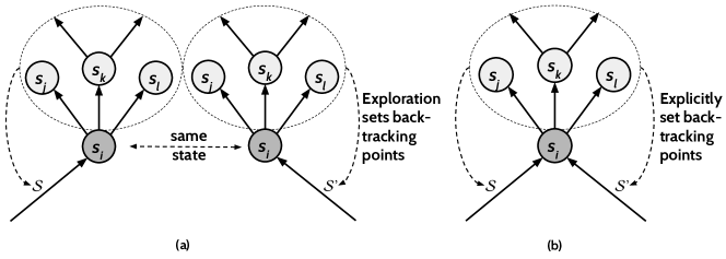
Figure 2: (a) Stateless model checking explores $s_{i}$, $s_{j}$, $s_{k}$, and $s_{l}$ twice and thus sets backtracking points for both $\mathcal{S}$ and $\mathcal{S}$’. (b) Stateful model checking matches state $s_{i}$ and skips the second exploration and thus we must explicitly set backtracking points.

4.2 Problem 2: State Matching for Previously Explored States

Typically stateful model checkers can simply terminate an execution when a previously discovered state is reached. As mentioned in [60], this handling is unsound in the presence of dynamic partial order reduction. Figure 2 illustrates the issue: Figure 2-a and b show the behavior of a classical stateless DPOR algorithm as well as the situation in a stateful DPOR algorithm, respectively. We assume that $\mathcal{S}$ was the first transition sequence to reach $s_{i}$ and $\mathcal{S}$’ was the second such transition sequence. The issue in Figure 2-b is that after the state match for $s_{i}$ in $\mathcal{S}$’, the algorithm may inappropriately skip setting backtracking points for the transition sequence $\mathcal{S}$’, preventing the model checker from completely exploring the state space.

Our Idea. Similar to the approach of Yang et al. [60], we propose to use a graph to store the set of previously explored transitions that may set backtracking points in the current transition sequence, so that the algorithm can set those backtracking points without reexploring the same state space.

4.3 Problem 3: State Matching Incompletely Explored States

⬇ // e4: if (x==0) { if (y==1) assert(y==0); } else { x = 0; }

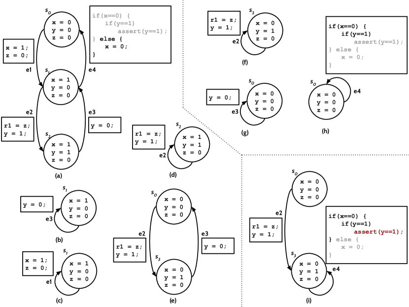
Figure 3: Example of a event-driven program that misses an execution. We assume that e1, e2, e3, and e4 are all initially enabled.

Figure 3 illustrates another problem with cyclic state spaces—even if our new termination condition and the algorithm for setting backtrack points for a state match are applied to the stateful DPOR algorithm, it could still fail to explore all executions.

With our new termination criteria, the stateful DPOR algorithm will first explore the execution shown in Figure 3-a. It starts from $s_{0}$ and executes the events e₁, e₂, and e₃. While executing the three events, it puts event e₂ in the backtrack set of $s_{0}$ and event e₃ in the backtrack set of $s_{1}$ as it finds a conflict between the events e₁ and e₂, and the events e₂ and e₃. Then, the algorithm revisits $s_{1}$. At this point it updates the backtrack sets using the transitions that are reachable from state $s_{1}$: it puts event e₂ in the backtrack set of state $s_{2}$ because of a conflict between e₂ and e₃.

However, with the new termination criteria, it does not stop its exploration. It continues to execute event e₄, finds a conflict between e₁ and e₄, and puts event e4 into the backtrack set of $s_{0}$. The algorithm now revisits state $s_{0}$ and updates the backtrack sets using the transitions reachable from state $s_{0}$: it puts event e₁ in the backtrack set of $s_{1}$ because of the conflict between e₁ and e₄. Figures 3-b, c, and d show the executions explored by the stateful DPOR algorithm from the events e₁ and e₃ in the backtrack set of $s_{1}$, and event e₂ in the backtrack set of $s_{2}$, respectively.

Next, the algorithm explores the execution from event e₂ in the backtrack set of $s_{0}$ shown in Figure 3-e. The algorithm finds a conflict between the events e₂ and e₃, and it puts event e₂ in the backtrack set of $s_{3}$ and event e₃ in the backtrack set of $s_{0}$ whose executions are shown in Figures 3-f and g, respectively. Finally, the algorithm explores the execution from event e₄ in the backtrack set of $s_{0}$ shown in Figure 3-h. Then the algorithm stops, failing to explore the asserting execution shown in Figure 3-i.

The key issue in the above example is that the stateful DPOR algorithm by Yang et al. [60] does not consider all possible transition sequences that can reach the current state but merely considers the current transition sequence when setting backtracking points. It thus does not add event e₄ from the execution in Figure 3-h to the backtrack set of state $s_{3}$.

Our Idea. Figure 4 shows the core issue behind the problem. When the algorithm sets backtracking points after executing the transition $t_{k}$, the algorithm must consider both the transition sequence that includes $t_{h}$ and the transition sequence that includes $t_{i}$. The classical backtracking algorithm would only consider the current transition sequence when setting backtracking points.

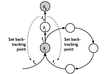
Figure 4: Stateful model checking needs to handle loops caused by cyclic state spaces.

We propose a new algorithm that uses a backwards depth first search on the state transition graph combined with summaries to set backtracking points on previously discovered paths to the currently executing transition. Yi et al. [62] uses a different approach for updating summary information to address this issue.

4.4 Problem 4: Events as Transitions

The fourth problem, also identified in Jensen et al. [22], is that existing stateful DPOR algorithms and most DPOR algorithms assume that each transition only executes a single memory operation, whereas an event in our context can consist of many different memory operations. For example, the e₄ handler in Figure 3 reads x and y.

A related issue is that many DPOR algorithms assume that they know, ahead of time, the effects of the next step for each thread. In our setting, however, since events contain many different memory operations, we must execute an event to know its effects. Figure 5 illustrates this problem. In this example, we assume that each event can only execute once.

⬇ /* e3: */ if (x==1) assert(y == 1);

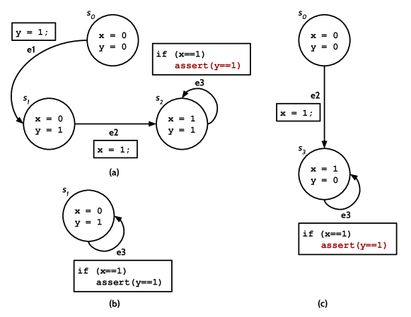
Figure 5: Example of an event-driven program for which a naive application of the standard DPOR algorithm fails to construct the correct persistent set at state $s_{0}$. We assume that e1, e2, and e3 are all initially enabled.

Figure 5-a shows the first execution of these 3 events. The stateful DPOR algorithm finds a conflict between the events e₂ and e₃, adds event e₃ to the backtrack set for state $s_{1}$, and then schedules the second execution shown in Figure 5-b. At this point, the exploration stops prematurely, missing the assertion violating execution shown in Figure 5-c.

The key issue is that the set $\{\text{\tt e${}_{1}$}\}$ is not a persistent set for state $s_{0}$. Traditional DPOR algorithms fail to construct the correct persistent set at state $s_{0}$ because the backtracking algorithm finds that the transition for event e₃ conflicts with the transition for event e₂ and stops setting backtracking points. This occurs since these algorithms do not separately track conflicts from different memory operations in an event when adding backtracking points—they simply assume transitions are comprised of single memory operations. Separately tracking different operations would allow these algorithms to find a conflict relation between the events e₁ and e₃ (as both access the variable y) in the first execution, put event e₂ into the backtrack set of $s_{0}$, and explore the missing execution shown in Figure 5-c.

Our Idea. In the classical DPOR algorithm, transitions correspond to single instructions whose effects can be determined ahead of time without executing the instructions [12]. Thus, the DPOR algorithm assumes that the effects of each thread’s next transition are known. Our events on the other hand include many instructions, and thus, as Jensen et al. [22] observes, determining the effects of an event requires executing the event. Our algorithm therefore determines the effects of a transition when the transition is actually executed.

A second consequence of having events as transitions is that transitions can access multiple different memory locations. Thus, as the example in Figure 5 shows, it does not suffice to simply set a backtracking point at the last conflicting transition. To address this issue, our idea is to compute conflicts on a per-memory-location basis.

5 Stateful Dynamic Partial Order Reduction

This section presents our algorithm, which extends DPOR to support stateful model checking of event-driven applications with cyclic state spaces. We first present the states that our algorithm maintains:

1. The transition sequence $\mathcal{S}$ contains the new transitions that the current execution explores. Our algorithm explores a given transition in at most one execution.

2. The state history $\mathcal{H}$ is a set of program states that have been visited in completed executions.

3. The state transition graph $\mathcal{R}$ records the states our algorithm has explored thus far. Nodes in this graph correspond to program states and edges to transitions between program states.

1 $\textsc{ExploreAll}{(}{)}$

2       $\hbox{$\mathcal{H}$}:=\emptyset$

3       $\hbox{$\mathcal{R}$}:=\emptyset$

4       $\hbox{$\mathcal{S}$}:=\emptyset$

5       $\textsc{Explore}{(}\hbox{$s_{0}$}{)}$

6       while $\exists\hbox{$s$},\>\hbox{{backtrack}}(\hbox{$s$})\neq\hbox{{done}}(\hbox{$s$})$ do

7             $\textsc{Explore}{(}\hbox{$s$}{)}$

8            

9       end while

10      

11 end

12

Algorithm 1 Top-level exploration algorithm.

1 $\textsc{Explore}{(}\hbox{$s$}{)}$

2       if $\hbox{{backtrack}}(\hbox{$s$})=\hbox{{done}}(\hbox{$s$})$ then

3             if $\hbox{{done}}(\hbox{$s$})=\hbox{{enabled}}(\hbox{$s$})$ then

4                   if $\hbox{{enabled}}(\hbox{$s$})\text{ is not empty}$ then

5                         $\text{select}\>\hbox{$e$}\>\in\hbox{{enabled}}(\hbox{$s$})$

6                         $\text{remove}\>\hbox{$e$}\>\text{from}\>\hbox{{done}}(\hbox{$s$})$

7                        

8                   else

9                         $\text{add}\>\hbox{\emph{states}}{}(\hbox{$\mathcal{S}$})\>\text{to}\>\hbox{$\mathcal{H}$}$

10                         $\hbox{$\mathcal{S}$}:=\emptyset$

11                         return

12                   end if

13                  

14             else

15                   $\text{select}\>\hbox{$e$}\>\in\hbox{{enabled}}(\hbox{$s$})\setminus\hbox{{done}}(\hbox{$s$})$

16                   $\text{add}\>\hbox{$e$}\>\text{to}\>\hbox{{backtrack}}(\hbox{$s$})$

17                  

18             end if

19            

20       end if

21       while $\exists\hbox{$b$}\in\hbox{{backtrack}}(\hbox{$s$})\setminus\hbox{{done}}(\hbox{$s$})$ do

22             $\text{add}\>\hbox{$b$}\>\text{to}\>\hbox{$s$}.done$

23             $\hbox{$t$}:=\text{\hbox{\emph{next}}}\left(\hbox{$s$},\hbox{$b$}\right)$

24             $\hbox{$s$}^{\prime}:=\hbox{\emph{dst}}\left(\hbox{$t$}\right)$

25             add transition $t$ to $\mathcal{R}$

26             foreach $\hbox{$e$}\in\hbox{{enabled}}(\hbox{$s$})\setminus\hbox{{enabled}}(\hbox{$s$}^{\prime})$  do

27                   $\text{add}\>\hbox{$e_{\>}$}\text{to}\>\hbox{{backtrack}}(\hbox{$s$})$

28                  

29             end foreach

30            $\textsc{UpdateBacktrackSet}\left(\hbox{$t$}\right)$

31             if $\hbox{$s$}^{\prime}\in\hbox{$\mathcal{H}$}\vee\textsc{IsFullCycle}\left(\hbox{$t$}\right)$ then

32                   $\textsc{UpdateBacktrackSetsFromGraph}\left(\hbox{$t$}\right)$

33                   $\text{add}\>\hbox{\emph{states}}{}(\hbox{$\mathcal{S}$})\>\text{to}\>\hbox{$\mathcal{H}$}$

34                   $\hbox{$\mathcal{S}$}:=\emptyset$

35                  

36             else

37                   if $\hbox{$s$}^{\prime}\in\hbox{\emph{states}}{}(\hbox{$\mathcal{S}$})$ then

38                         $\textsc{UpdateBacktrackSetsFromGraph}\left(\hbox{$t$}\right)$

39                   end if

40                  $\hbox{$\mathcal{S}$}:=\hbox{$\mathcal{S}$}.\hbox{$t$}$

41                   $\textsc{Explore}{(}\hbox{$s$}^{\prime}{)}$

42                  

43             end if

44            

45       end while

46      

47 end

48

Algorithm 2 Stateful DPOR algorithm for event-driven applications.

Recall that for each reachable state $\hbox{$s$}\in\hbox{$\textit{States}$}{}$, our algorithm maintains the $\hbox{{backtrack}}(\hbox{$s$})$ set that contains the events to be explored at $s$, the $\hbox{{done}}(\hbox{$s$})$ set that contains the events that have already been explored at $s$, and the $\hbox{{enabled}}(\hbox{$s$})$ set that contains all events that are enabled at $s$.

Algorithm 1 presents the top-level ExploreAll procedure. This procedure first invokes the Explore procedure to start model checking from the initial state. However, the presence of cycles in the state space means that our backtracking-based search algorithm may occasionally set new backtracking points for states in completed executions. The ExploreAll procedure thus loops over all states that have unexplored items in their backtrack sets and invokes the Explore procedure to explore those transitions.

Algorithm 2 describes the logic of the Explore procedure. The if statement in line 2 checks if the current state $s$’s backtrack set is the same as the current state $s$’s done set. If so, the algorithm selects an event to execute in the next transition. If some enabled events are not yet explored, it selects an unexplored event to add to the current state’s backtrack set. Otherwise, if the enabled set is not empty, it selects an enabled event to remove from the done set. Note that this scenario occurs only if the execution is continuing past a state match to satisfy the termination condition.

Then the while loop in line 2 selects an event $b$ to execute on the current state $s$ and executes the event $b$ to generate the transition $t$ that leads to a new state $\hbox{$s$}^{\prime}$. At this point, the algorithm knows the memory accesses performed by the transition $t$ and thus can add the event $b$ to the backtrack sets of the previous states. This is done via the procedure UpdateBacktrackSet.

Traditional DPOR algorithms continue an execution until it terminates. Since our programs may have cyclic state spaces, this would cause the model checker to potentially not terminate. Our algorithm instead checks the conditions in line 2 to decide whether to terminate the execution. These checks see whether the new state $\hbox{$s$}^{\prime}$ matches a state from a previous execution, or if the current execution revisits a state the current execution previously explored and meets other criteria that are checked in the IsFullCycle procedure. If so, the algorithm calls the UpdateBacktrackSetsFromGraph procedure to set backtracking points, from transitions reachable from $t$, to states that can reach $t$. An execution will also terminate if it reaches a state in which no event is enabled (line 2). It then adds the states from the current transition sequence to the set of previously visited states $\mathcal{H}$, resets the current execution transition sequence $\mathcal{S}$, and backtracks to start a new execution.

If the algorithm has reached a state $\hbox{$s$}^{\prime}$ that was previously discovered in this execution, it sets backtracking points by calling the UpdateBacktrackSetsFromGraph procedure. Finally, it updates the transition sequence $\mathcal{S}$ and calls Explore.

1 $\textsc{UpdateBacktrackSetsFromGraph}{(}\hbox{$t_{s}$}{)}$

2       $\hbox{$\mathcal{R}_{t}$}:=\{\hbox{$t$}\in\hbox{$\mathcal{R}$}\mid\>\>\hbox{$t_{s}$}\hbox{$\>\rightarrow_{r}\>$}\hbox{$t$}\}$

3       foreach $\hbox{$t$}\in\hbox{$\mathcal{R}_{t}$}$ do

4             $\textsc{UpdateBacktrackSet}\left(\hbox{$t$}\right)$

5            

6       end foreach

7      

8 end

9

Algorithm 3 Procedure that updates the backtrack sets of states in previous executions.

Algorithm 3 shows the UpdateBacktrackSetsFromGraph procedure. This procedure takes a transition $t$ that connects the current execution to a previously discovered state in the transition graph $\mathcal{R}$. Since our algorithm does not explore all of the transitions reachable from the previously discovered state, we need to set the backtracking points that would have been set by these skipped transitions. This procedure therefore computes the set of transitions reachable from the destination state of $t$ and invokes UpdateBacktrackSet on each of those transitions to set backtracking points.

1 $\textsc{IsFullCycle}{(}\hbox{$t$}{)}$

2       if $\neg\textit{dst}(\hbox{$t$})\in\hbox{\emph{states}}{}(\hbox{$\mathcal{S}$})$ then

3            return false

4       end if

5      $\hbox{$\mathcal{S}$}^{\textit{fc}}:=\{\hbox{$t_{j}$}\in\hbox{$\mathcal{S}$}\mid i=\hbox{\emph{first}}(\hbox{$\mathcal{S}$},\hbox{\emph{dst}}(\hbox{$t$})),\>\>\text{and}\>\>i<j\}\cup\{\hbox{$t$}\}$

6       $\hbox{$\mathcal{E}_{\textit{fc}}$}:=\{\hbox{\emph{event}}{}(\hbox{$t$}^{\prime})\mid\forall\hbox{$t$}^{\prime}\in\hbox{$\mathcal{S}$}^{\textit{fc}}\>\}$

7       $\hbox{$\mathcal{E}_{\textit{enabled}}$}:=\{\hbox{{enabled}}(\hbox{\emph{dst}}{}(\hbox{$t$}^{\prime}))\mid\forall\hbox{$t$}^{\prime}\in\hbox{$\mathcal{S}$}^{\textit{fc}}\>\}$

8       return $\hbox{$\mathcal{E}_{\textit{fc}}$}=\hbox{$\mathcal{E}_{\textit{enabled}}$}\>$

9 end

10

Algorithm 4 Procedure that checks the looping termination condition: a cycle that contains every event enabled in the cycle.

Algorithm 4 presents the IsFullCycle procedure. This procedure first checks if there is a cycle that contains the transition $t$ in the state space explored by the current execution. The example from Figure 1 shows that such a state match is not sufficient to terminate the execution as the execution may not have set the necessary backtracking points. Our algorithm stops the exploration of an execution when there is a cycle that has explored every event that is enabled in that cycle. This ensures that for every transition $t$ in the execution, there is a future transition $t_{e}$ for each enabled event $e$ in the cycle that can set a backtracking point if $t$ and $t_{e}$ conflict.

Algorithm 5 presents the UpdateBacktrackSet procedure, which sets backtracking points. There are two differences between our algorithm and traditional DPOR algorithms. First, since our algorithm supports programs with cyclic state spaces, it is possible that the algorithm has discovered multiple paths from the start state $s_{0}$ to the current transition $t$. Thus, the algorithm must potentially set backtracking points on multiple different paths. We address this issue using a backwards depth first search traversal of the $\mathcal{R}$ graph. Second, since our transitions correspond to events, they may potentially access multiple different memory locations and thus the backtracking algorithm potentially needs to set separate backtracking points for each of these memory locations.

The UpdateBacktrackSetDFS procedure implements a backwards depth first traversal to set backtracking points. The procedure takes the following parameters: $t_{\text{curr}}$ is the current transition in the DFS, $t_{\text{conf}}$ is the transition that we are currently setting a backtracking point for, $\mathcal{A}$ is the set of accesses that the algorithm searches for conflicts for, and $\mathcal{T}_{\text{exp}}$ is the set of transitions that the algorithm has explored down this search path. Recall that accesses consist of both an operation, i.e., a read or write, and a memory location. Conflicts are defined in the usual way—writes to a memory location conflict with reads or writes to the same location.

1 $\textsc{UpdateBacktrackSet}{(}\hbox{$t$}{)}$

2       $\textsc{UpdateBacktrackSetDFS}\left(\hbox{$t$},\hbox{$t$},\textit{accesses}(\hbox{$t$}),\{\hbox{$t$}\}\right)$

3 end

4

5 $\textsc{UpdateBacktrackSetDFS}{(}\hbox{$t_{\text{curr}}$},\hbox{$t_{\text{conf}}$},\hbox{$\mathcal{A}$},\hbox{$\mathcal{T}_{\text{exp}}$}{)}$

6       foreach $\hbox{$t_{b}$}\in\textit{pred}_{\hbox{$\mathcal{R}$}}(\hbox{$t_{\text{curr}}$})\setminus\hbox{$\mathcal{T}_{\text{exp}}$}$ do

7             $\hbox{$\mathcal{A}_{b}$}:=\textit{accesses}(\hbox{$t_{b}$})$

8             $\hbox{$t_{\text{conf}}$}^{\prime}:=\hbox{$t_{\text{conf}}$}$

9             if $\exists a\in\hbox{$\mathcal{A}$},\exists a_{b}\in\hbox{$\mathcal{A}_{b}$},\hbox{{conflicts}}(a,a_{b})$ then

10                   if $\hbox{\emph{event}}(\hbox{$t_{\text{conf}}$})\in\hbox{{enabled}}(\hbox{\emph{src}}(\hbox{$t_{b}$}))$ then

11                         $\text{add}\>\hbox{\emph{event}}(\hbox{$t_{\text{conf}}$})\>\text{to}\>\hbox{{backtrack}}(\hbox{\emph{src}}(\hbox{$t_{b}$}))$

12                        

13                   else

14                         $\text{add}\>\hbox{{enabled}}(\hbox{\emph{src}}(\hbox{$t_{b}$}))\>\text{to}\>\hbox{{backtrack}}(\hbox{\emph{src}}(\hbox{$t_{b}$}))$

15                        

16                   end if

17                  $\hbox{$t_{\text{conf}}$}^{\prime}:=\hbox{$t_{b}$}$

18                  

19             end if

20            $\hbox{$\mathcal{A}_{r}$}:=\{a\in\hbox{$\mathcal{A}$}\mid\neg\exists a_{b}\in\hbox{$\mathcal{A}_{b}$},\hbox{{conflicts}}(a,a_{b})\}$

21             $\textsc{UpdateBacktrackSetDFS}\left(\hbox{$t_{b}$},\hbox{$t_{\text{conf}}$}^{\prime},\hbox{$\mathcal{A}_{r}$},\hbox{$\mathcal{T}_{\text{exp}}$}\>\cup\{\hbox{$t_{b}$}\}\right)$

22       end foreach

23      

24 end

25

Algorithm 5 Procedure that updates the backtrack sets of states for previously executed transitions that conflict with the current transition in the search stack.

Line 5 loops over each transition $t_{b}$ that immediately precedes transition $t_{\text{curr}}$ in the state transition graph and has not been explored. Line 5 checks for conflicts between the accesses of $t_{b}$ and the access set $\mathcal{A}$ for the DFS. If a conflict is detected, the algorithm adds the event for transition $t_{\text{conf}}$ to the backtrack set. Line 5 removes the accesses that conflicted with transition $t_{b}$. The search procedure then recursively calls itself. If the current transition $t_{b}$ conflicts with the transition $t_{\text{conf}}$ for which we are setting a backtracking point, then it is possible that the behavior we are interested in for $t_{\text{conf}}$ requires that $t_{b}$ be executed first. Thus, if there is a conflict between $t_{b}$ and $t_{\text{conf}}$, we pass $t_{b}$ as the conflict transition parameter to the recursive calls to UpdateBacktrackSetDFS.

Appendix 0.B proves correctness properties for our DPOR algorithm. Appendix 0.C revisits the example shown in Figure 3. It describes how our DPOR algorithm explores all executions in Figure 3, including Figure 3-i.

6 Implementation and Evaluation

In this section, we present the implementation of our DPOR algorithm (Section 6.1) and its evaluation results (Section 6.2).

6.1 Implementation

We have implemented the algorithm by extending IoTCheck [49], a tool that model-checks pairs of Samsung’s SmartThings smart home apps and reports conflicting updates to the same device or global variables from different apps. IoTCheck extends Java Pathfinder, an explicit stateful model checker [55]. In the implementation, we optimized our DPOR algorithm by caching the results of the graph search when UpdateBacktrackSetsFromGraph is called. The results are cached for each state as a summary of the potentially conflicting transitions that are reachable from the given state (see Appendix 0.D).

We selected the SmartThings platform because it has an extensive collection of event-driven apps. The SmartThings official GitHub [45] has an active user community—the repository has been forked more than 84,000 times as of August 2021.

We did not compare our implementation against other systems, e.g., event-driven systems [22, 30]. Not only that these systems do not perform stateful model checking and handle cyclic state spaces, but also they implemented their algorithms in different domains: web [22] and Android applications [30]—it will not be straightforward to adapt and compare these with our implementation on smart home apps.

6.2 Evaluation

Dataset. Our SmartThings app corpus consists of 198 official and third-party apps that are taken from the IoTCheck smart home apps dataset [48, 49]. These apps were collected from different sources, including the official SmartThings GitHub [45]. In this dataset, the authors of IoTCheck formed pairs of apps to study the interactions between the apps [49].

We selected the 1,438 pairs of apps in the Device Interaction category as our benchmarks set. It contains a diverse set of apps and app pairs that are further categorized into 11 subgroups based on various device handlers [44] used in each app. For example, the FireCO2Alarm [38] and the Lock-It-When-I-Leave [1] apps both control and may interact through a door lock (see Section 1). Hence, they are both categorized as a pair in the Locks group. As the authors of IoTCheck noted, these pairs are challenging to model check—IoTCheck did not finish for 412 pairs.

Table 1: Sample model-checked pairs that finished with or without DPOR. Evt. is number of events and Time is in seconds. The complete list of results for 229 pairs that finished with or without DPOR is included in Table A.2 in Appendices.

No.	App	Evt.	Without DPOR			With DPOR
			States	Trans.	Time	States	Trans.	Time
1	smart-nightlight–ecobeeAwayFromHome	14	16,441	76,720	5,059	11,743	46,196	5,498
2	step-notifier–ecobeeAwayFromHome	11	14,401	52,800	4,885	11,490	35,142	5,079
3	smart-security–ecobeeAwayFromHome	11	14,301	47,608	4,385	8,187	21,269	2,980
4	keep-me-cozy–whole-house-fan	17	8,793	149,464	4,736	8,776	95,084	6,043
5	keep-me-cozy-ii–thermostat-window-check	13	8,764	113,919	4,070	7,884	59,342	4,515
6	step-notifier–mini-hue-controller	6	7,967	47,796	2,063	7,907	40,045	3,582
7	keep-me-cozy–thermostat-mode-director	12	7,633	91,584	3,259	6,913	49,850	3,652
8	lighting-director–step-notifier	14	7,611	106,540	5,278	2,723	25,295	2,552
9	smart-alarm–DeviceTamperAlarm	15	5,665	84,960	3,559	3,437	40,906	4,441
10	forgiving-security–smart-alarm	13	5,545	72,072	3,134	4,903	52,205	5,728

Pair Selection. In the IoTCheck evaluation, the authors had to exclude 175 problematic pairs. In our evaluation, we further excluded pairs. First, we excluded pairs that were reported to finish their executions in 10 seconds or less—these typically will generate a small number of states (i.e., less than 100) when model checked. Next, we further removed redundant pairs across the different 11 subgroups. An app may control different devices, and thus they may use various device handlers in its code. For example, the apps FireCO2Alarm [38] and groveStreams [39] both control door locks and thermostats in their code. Thus, the two apps are categorized as a pair both in the Locks and Thermostats subgroups—we need to only include this pair once in our evaluation. These steps reduced our benchmarks set to 535 pairs.

Experimental Setup. Each pair was model checked on an Ubuntu-based server with Intel Xeon quad-core CPU of 3.5GHz and 32GB of memory—we allocated 28GB of heap space for JVM. In our experiments, we ran the model checker for every pair for at most 2 hours. We found that the model checker usually ran out of memory for pairs that had to be model checked longer. Further investigation indicates that these pairs generate too many states even when run with the DPOR algorithm. We observed that many smart home apps generate substantial numbers of read-write and write-write conflicts when model checked—this is challenging for any DPOR algorithms. In our benchmarks set, 300 pairs finished for DPOR and/or no DPOR.

Results. Our DPOR algorithm substantially reduced the search space for many pairs. There are 69 pairs that were unfinished (i.e., “Unf”) without DPOR. These pairs did not finish because their executions exceeded the 2-hour limit, or generated too many states quickly and consumed too much memory, causing the model checker to run out of memory within the first hour of their execution. When run with our DPOR algorithm, these pairs successfully finished—mostly in 1 hour or less. Table A.1 in Appendices shows the results for pairs that finished with DPOR but did not finish without DPOR. Most notably, even for the pair initial-state-event-streamer—thermostat-auto-off that has the most number of states, our DPOR algorithm successfully finished model checking it within 1 hour.

Next, we discovered that 229 pairs finished when model checked with and without DPOR. Table 1 shows 10 pairs with the most numbers of states (see the complete results in Table A.2 in Appendices). These pairs consist of apps that generate substantial numbers of read-write and write-write conflicts when model checked with our DPOR algorithm. Thus, our DPOR algorithm did not significantly reduce the states, transitions, and runtimes for these pairs.

Finally, we found 2 pairs that finished when run without our DPOR algorithm, but did not finish when run with it. These pairs consist of apps that are exceptionally challenging for our DPOR algorithm in terms of numbers of read-write and write-write conflicts. Nevertheless, these are corner cases—please note that our DPOR algorithm is effective in many pairs.

Overall, our DPOR algorithm achieved a 2$\times$ state reduction and a 3$\times$ transition reduction for the 229 pairs that finished for both DPOR and no DPOR (geometric mean). Assuming that “Unf” is equal to 7,200 seconds (i.e., 2 hours) of runtime, we achieved an overall speedup of 7$\times$ for the 300 pairs (geometric mean). This is a lower bound runtime for the “Unf” cases, in which executions exceeded the 2-hour limit—these pairs could have taken more time to finish.

7 Related Work

There has been much work on model checking. Stateless model checking techniques do not explicitly track which program states have been visited and instead focus on enumerating schedules [13, 14, 15, 33].

To make model checking more efficient, researchers have also looked into various partial order reduction techniques. The original partial order reduction techniques (e.g., persistent/stubborn sets [13, 52] and sleep sets [13]) can also be used in the context of cyclic state spaces when combined with a proviso that ensures that executions are not prematurely terminated [13], and ample sets [8, 7] that are basically persistent sets with additional conditions. However, the persistent/stubborn set techniques “suffer from severe fundamental limitation”[12]: the operations and their communication objects in future process executions are difficult or impossible to compute precisely through static analysis, while sleep sets alone only reduce the number of transitions (not states). Work on collapses by Katz and Peled also suffers from the same requirement for a statically known independence relation [23].

The first DPOR technique was proposed by Flanagan and Godefroid [12] to address those issues. The authors introduced a technique that combats the state space explosion by detecting read-write and write-write conflicts on shared variable on the fly. Since then, a significant effort has been made to further improve dynamic partial order reduction [42, 43, 26, 41, 47]. Unfortunately, a lot of DPOR algorithms assume the context of shared-memory concurrency in that each transition consists of a single memory operation. In the context of event-driven applications, each transition is an event that can consist of different memory operations. Thus, we have to execute the event to know its effects and analyze it dynamically on the fly in our DPOR algorithm (see Section 4.4).

Optimal DPOR [2] seeks to make stateless model checking more efficient by skipping equivalent executions. Maximal causality reduction [19] further refines the technique with the insight that it is only necessary to explore executions in which threads read different values. Value-centric DPOR [6] has the insight that executions are equivalent if all of their loads read from the same writes. Unfolding [40] is an alternative approach to POR for reducing the number of executions to be explored. The unfolding algorithm involves solving an NP-complete problem to add events to the unfolding.

Recent work has extended these algorithms to handle the TSO and PSO memory models [3, 63, 20] and the release acquire fragment of C/C++ [4]. The RCMC tool implements a DPOR tool that operates on execution graphs for the RC11 memory model [24]. SAT solvers have been used to avoid explicitly enumerating all executions. SATCheck extends partial order reduction with the insight that it is only necessary to explore executions that exhibit new behaviors [9]. CheckFence checks code by translating it into SAT [5]. Other work has also presented techniques orthogonal to DPOR, either in a more general context [10] or platform specific (e.g., Android [36] and Node.js [29]).

Recent work on dynamic partial order reduction for event-driven programs has developed dynamic partial order reduction algorithms for stateless model checking of event-driven applications [22, 30]. Jensen et al. [22] consider a model similar to ours in which an event is treated as a single transition, while Maiya et al. [30] consider a model in which event execution interleaves concurrently with threads. Neither of these approaches handle cyclic state spaces nor consider challenges that arise from stateful model checking.

Recent work on DPOR algorithms reduces the number of executions for programs with critical sections by considering whether critical sections contain conflicting operations [25]. This work considers stateless model checking of multithreaded programs, but like our work it must consider code blocks that perform multiple memory operations.

CHESS [33] is designed to find and reproduce concurrency bugs in C, C++, and C#. It systematically explores thread interleavings using a preemption bounded strategy. The Inspect tool combines stateless model checking and stateful model checking to model check C and C++ code [61, 56, 59].

In stateful model checking, there has also been substantial work such as SPIN [18], Bogor [11], and JPF [55]. In addition to these model checkers, other researchers have proposed different techniques to capture program states [32, 17].

Versions of JPF include a partial order reduction algorithm. The design of this algorithm is not well documented, but some publications have reverse engineered the pseudocode [34]. The algorithm is naive compared to modern DPOR algorithms—this algorithm simply identifies accesses to shared variables and adds backtracking points for all threads at any shared variable access.

8 Conclusion

In this paper, we have presented a new technique that combines dynamic partial order reduction with stateful model checking to model check event-driven applications with cyclic state spaces. To achieve this, we introduce two techniques: a new termination condition for looping executions and a new algorithm for setting backtracking points. Our technique is the first stateful DPOR algorithm that can model check event-driven applications with cyclic state spaces. We have evaluated this work on a benchmark set of smart home apps. Our results show that our techniques effectively reduce the search space for these apps. This is the extended version of our paper, with the same title, published at VMCAI 2022.

Appendices

Appendix 0.A Example Event-Driven System

Figure A.1 depicts components of an example event-driven system. The application SmartLightApp in the figure is developed using this concurrency model and may run in the cloud. It has a fixed set of events that are associated with it and their respective event handlers. It also has logic to decide whether to perform specific actions based on the triggering events. For example, SmartLightApp can turn on and off a light bulb based on specific triggers.

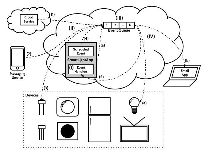
Figure A.1: Example Event-driven System.

Our example event-driven system has the following 4 components:

(I) Event handlers: The application code is composed of a set of event handlers. Each event handler processes a certain class of events. When the event handler executes, it receives the appropriate event object. When the runtime system dequeues an event $e$, it executes the relevant event handler.

(II) External events: An application can have a number of sources that deliver triggering events: (1) a cloud service (e.g., a cloud service that reports the current outdoor temperature), (2) a service that is running on a computing device (e.g., a messaging service that sends a trigger whenever there is an incoming message), (3) a device (e.g., an illuminance sensor that sends a trigger whenever there is a change of light intensity in its environment), (4) a scheduled event within the application (e.g., turn on a light bulb at 6pm), or (5) an event generated by the application that triggers another component of that app: these events potentially change the app’s state (e.g., a scheduled mode change to night may trigger a light bulb to turn on).

(III) Internal events: An application can directly generate events, for example to: (a) actuate a certain device (e.g., turn on a light bulb) or (b) trigger another app running on a computing device (e.g., trigger an email to be sent from an email app).

(IV) Event queue: All events are pushed into an event queue to be delivered by the runtime to the appropriate event handlers.

Examples of platforms with this event-driven model include the Samsung SmartThings platform [46, 45], a popular platform used to create apps that control devices to automate tasks for a smart home.

Appendix 0.B Correctness

This section proves the correctness of our stateful DPOR algorithm with the following proof strategy: we first prove that the stateless analog of our dynamic partial order reduction algorithm is correct in Theorem 0.B.1. We then prove that the stateful algorithm explores all transitions that the stateless algorithm explores.

Given a transition sequence $\mathcal{S}$, we use the following notations in our proof:

• $\lvert\hbox{$\mathcal{S}$}\rvert$ returns the length of $\mathcal{S}$.

• $\mathcal{S}_{i}$ denotes the $i$-th transition in $\mathcal{S}$, and $\mathcal{S}_{i...j}$ denotes the subsequence of $\mathcal{S}$ from the $i$-th position to the $j$-th position.

We also define the notion of transitive dependence as follows:

Definition 4 (Transitive Dependence)

Given a transition sequence $\tau$: $\hbox{$s_{0}$}\xrightarrow{\hbox{$t_{1}$}}\hbox{$s_{1}$}\xrightarrow{\hbox{$t_{2}$}}\hbox{$s_{2}$}...\xrightarrow{\hbox{$t_{n-1}$}}\hbox{$s_{n-1}$}\xrightarrow{\hbox{$t_{n}$}}\hbox{$s_{n}$}$, the transitive dependence relation $\rightarrow_{\tau}$ is the smallest partial order on $\tau$ such that if $i<j$ and $t_{i}$ is dependent on $t_{j}$, then $\hbox{$t_{i}$}\rightarrow_{\tau}\hbox{$t_{j}$}$.

The notion of transitive dependence enables partial order reduction. The transition sequence $\tau$ is one linearization of the partial order $\rightarrow_{\tau}$. A search algorithm only needs to explore one linearization, because other linearizations of $\rightarrow_{\tau}$ yield “equivalent” transition sequences of $\tau$, which can be obtained by swapping adjacent independent transitions.

0.B.1 Correctness of the Stateless Algorithm

For the stateless analog of the algorithm, the if conditions in lines 2 and 2 of Algorithm 2 are always false, and the data structures $\mathcal{S}$ and $\mathcal{H}$ in Algorithm 1 and 2 are don’t-care terms. When all events in $\hbox{{backtrack}}(\hbox{$s$})$ have been explored, the search from $s$ is over, and we say that the state $s$ is “backtracked”.

Theorem 0.B.1

Let $\mathcal{E}$ be a finite set of events, $\tau$ be a transition sequence from the initial state $s_{0}$ explored by the stateless analog of the algorithm in an acyclic transition system, and $\hbox{$s_{0}$}\xrightarrow{\tau}\hbox{$s$}$. Then, when $s$ is backtracked,

1. the set of events that have been explored from $s$ is a persistent set in $s$, and

2. every trace $\tau\cdot\lambda$ in the state space of $A_{G}$ is a prefix of a linearization of $\rightarrow_{\tau\cdot\lambda^{\prime}}$ for some explored trace $\tau\cdot\lambda^{\prime}$.

Proof

Acyclicity implies that the system satisfies the descending chain condition, and we can apply well-founded induction. We need to prove the statements for the trace $\hbox{$s_{0}$}\xrightarrow{\tau}\hbox{$s$}$, assuming that the statements hold for all longer traces $\hbox{$s_{0}$}\xrightarrow{\tau}\hbox{$s$}\xrightarrow{\tau^{\prime}}\hbox{$s$}^{\prime}$, where $\hbox{$s$}^{\prime}$ is reachable from $s$ in finite steps.

Let $T:=\hbox{{backtrack}}(\hbox{$s$})$. For the first statement, i.e., $T$ is a persistent set when $s$ is backtracked, we will prove it by contradiction. If $T$ is not a persistent set, then there must exist a transition sequence from $s$,

$$\hbox{$s$}\xrightarrow{\hbox{$t_{1}$}}\hbox{$s_{1}$}\xrightarrow{\hbox{$t_{2}$}}\hbox{$s_{2}$}...\xrightarrow{\hbox{$t_{n-1}$}}\hbox{$s_{n-1}$}\xrightarrow{\hbox{$t_{n}$}}\hbox{$s_{n}$},$$

where $\hbox{\emph{event}}{(\hbox{$t_{1}$})},...,\hbox{\emph{event}}{(\hbox{$t_{n}$})}\notin T$, events $\hbox{\emph{event}}{(\hbox{$t_{1}$})},...,\hbox{\emph{event}}{(\hbox{$t_{n-1}$})}$ are read-write independent with all events in $T$, and $\hbox{\emph{event}}{(\hbox{$t_{n}$})}$ is dependent with some $x\in T$ at state $s_{n-1}$. Select the shortest such transition sequence. Let $\sigma$ be the transition sequence $\hbox{$t_{1}$}...\hbox{$t_{n-1}$}$. For simplicity, we will label $\hbox{\emph{event}}(\hbox{$t_{i}$})$ as $\tilde{e}_{i}$ for $1\leq i\leq n$. Note that $\tilde{e}_{i}$ and $\tilde{e}_{j}$ could be the same event even if $i\neq j$.

Since $x$ is read-write independent with $\tilde{e}_{i}$ for all $1\leq i\leq n-1$, we have the following transition diagram:

There are two cases: (1) $\tilde{e}_{n}$ is enabled in $s$; and (2) $\tilde{e}_{n}$ is disabled in $s$.

Case 1: Suppose that $\tilde{e}_{n}$ is enabled in $s$ but disabled in $\hbox{$s$}^{\prime}$. Since $x\in T$ and $\hbox{$s$}\xrightarrow{x}\hbox{$s$}^{\prime}$ has been explored when $s$ is backtracked, the for loop at line 2 of Algorithm 2 will add $\tilde{e}_{n}$ to $T$, contradicting the assumption that $\hbox{$\tilde{e}_{n}$}\notin T$.

Suppose that $\tilde{e}_{n}$ is enabled in $s$ and $\hbox{$s$}^{\prime}$. Then, $x$ does not enable or disable $\tilde{e}_{n}$. Since $x$ is read-write independent with all corresponding events in $\sigma$, $\tilde{e}_{n}$ is also enabled in $\hbox{$s_{n-1}$}^{\prime}$. Recall that $\tilde{e}_{n}$ is dependent with $x$ at $s_{n-1}$. Since $x$ does not enable or disable $\tilde{e}_{n}$, $x$ and $\tilde{e}_{n}$ must have conflicting memory accesses $\mathcal{A}_{x,n}$ in the transition sequence $\tau\cdot\sigma\cdot\hbox{$t_{x}$}\cdot\hbox{$t_{n}$}$, which is equivalent to the transition sequence $\tau\cdot\hbox{$t_{x}$}\cdot\sigma\cdot\hbox{$t_{n}$}$, where $\hbox{\emph{event}}({\hbox{$t_{x}$}})=x$. Since $x\in T$ and by the inductive assumption, we have explored some transition sequence $\tilde{\tau}$ where some linearization of $\rightarrow_{\tilde{\tau}}$ has prefix $\tau\cdot\hbox{$t_{x}$}\cdot\sigma\cdot\hbox{$t_{n}$}$. Thus, line 2 in Algorithm 2 would have called UpdateBacktrackSet and found the conflicting memory accesses $\mathcal{A}_{x,n}$, which is not empty until some $\tilde{e}_{i}$ is added to $T$. Thus, we have a contradiction.

Case 2: Suppose that $\tilde{e}_{n}$ is disabled in $s$. Since $\tilde{e}_{n}$ is enabled in $s_{n-1}$, there exists some transition $t_{i}$ in $\sigma$ that writes to the shadow location of $\tilde{e}_{n}$. Since $x$ is read-write independent with $\hbox{$\tilde{e}_{1}$},...,\hbox{$\tilde{e}_{n-1}$}$ by assumption, $x$ does not write to the shadow location of $\tilde{e}_{n}$, i.e., $x$ does not enable or disable $\tilde{e}_{n}$. Then, $\tilde{e}_{n}$ is also enabled in $\hbox{$s_{n-1}$}^{\prime}$. Therefore, the same argument in the second paragraph of Case 1 applies, and we have a contradiction.

We have shown that $T$ is a persistent set. We now move to prove the second statement in this theorem, that every trace $\hbox{$s_{0}$}\xrightarrow{\tau}\hbox{$s$}\xrightarrow{\lambda}u$ is a prefix of a linearization of $\rightarrow_{\tau\cdot\lambda^{\prime}}$ for some explored trace $\tau\cdot\lambda^{\prime}$. If $\lambda$ is the null sequence, then we are done, because $\hbox{$s_{0}$}\xrightarrow{\tau}\hbox{$s$}$ is already explored.

Let $\lambda=\pi\cdot\eta$, where $\pi$ is the maximal transition sequence such that no events executed in $\pi$ is in $T$. If $\eta$ is not the null sequence, then the first transition in $\eta$, denoted by $\eta_{1}$, is in $T$. Since $T$ is a persistent set, $\eta_{1}$ is independent with all transitions in $\pi$. Thus, $\tau\cdot\pi\cdot\eta$ is equivalent to $\tau\cdot\eta_{1}\cdot\pi\cdot\eta_{2...\lvert\eta\rvert}$. Note that $\tau\cdot\eta_{1}$ is a transition sequence that is explored by the algorithm. Thus, by the inductive assumption, $\tau\cdot\eta_{1}\cdot\pi\cdot\eta_{2...\lvert\eta\rvert}$ is a prefix of a linearization of $\rightarrow_{\tau\cdot\eta_{1}\cdot\lambda^{\prime}}$ for some explored trace $\tau\cdot\eta_{1}\cdot\lambda^{\prime}$. Then, $\tau\cdot\lambda=\tau\cdot\pi\cdot\eta$ is a prefix of another linearization of $\rightarrow_{\tau\cdot\eta_{1}\cdot\lambda^{\prime}}$. The same argument holds if $\pi$ is the null sequence.

Let $\eta$ be the null sequence. Pick $y\in T$. Then, $\tau\cdot\hbox{$t_{y}$}$ is an explored transition sequence, where $\hbox{\emph{event}}(\hbox{$t_{y}$})=y$. The inductive assumption implies that $\tau\cdot\hbox{$t_{y}$}\cdot\pi$ is a prefix of a linearization of $\rightarrow_{\tau\cdot t_{y}\cdot\lambda^{\prime}}$ for some explored trace $\tau\cdot\hbox{$t_{y}$}\cdot\lambda^{\prime}$. Because $t_{y}$ is independent with all transitions in $\pi$, $\tau\cdot\pi\cdot\hbox{$t_{y}$}$ is also a prefix of some linearization of $\rightarrow_{\tau\cdot t_{y}\cdot\lambda^{\prime}}$. Hence, $\tau\cdot\pi$ is a prefix of some linearization of $\rightarrow_{\tau\cdot t_{y}\cdot\lambda^{\prime}}$ as well.

0.B.2 Correctness of the Stateful Algorithm

Theorem 0.B.1 assumes that the transition system $A_{G}$ has an acyclic state space. In general, we do not expect our programs to have acyclic state spaces. Therefore, we make an acyclic version of $A_{G}$ by constructing a $k$-bounded instantiation of the transition system $A_{G}$ in which each event can run at most $k$ times. This is equivalent to transforming the program to add a counter per event type that permanently disables an event after the event handler has been executed $k$ times. Definition 5 formalizes the notion of the $k$-bounded instantiation. This would conceptually be implemented by adding a separate mechanism to the algorithm that only adds events that have not reached their $k$ bound to the backtrack set and would not add events that have reached their $k$ bound to the backtrack set in line 2 of Algorithm 2.

Definition 5 (Strictly k-Bounded Instantiation)

A $k$-bounded instantiation of a transition system $A_{G}$ is a program, where the execution continues until it reaches a state, in which all enabled events have run $k$ times.

We then will demonstrate the correctness of the results of a run of the stateful algorithm on the original, unbounded transition system $A_{G}$ by showing that for any arbitrary $k$, there exists a run of the stateless algorithm on a $k$-bounded instantiation of $A_{G}$ that explores a subset of transitions explored by the stateful algorithm on the original transition system. Our strict, local notion of a $k$-bounded instantiation of $A_{G}$ is not sufficient to show this because the stateful algorithm could select an event $e$ to execute at state $s$ that has already reached its $k$-bound while there exist other events that have not reached their $k$-bound. Therefore, we define a looser notion of a $k$-bounded instantiation of $A_{G}$ in Definition 6.

Definition 6 (Loosely k-Bounded Instantiation)

A loosely $k$-bounded instantiation of a transition system $A_{G}$ is a program, where the execution continues until it reaches a state, in which all enabled events have run at least $k$ times.

We define a run of the stateful or stateless algorithm as a full invocation of the ExploreAll procedure, which explores different executions of the targeted program. There can be multiple runs of the stateless algorithm on a bounded instantiation of $A_{G}$, because adding to and extracting events from the backtrack sets are non-deterministic in lines 2, 2 and 2 of Algorithm 2. However, Theorem 0.B.1 shows that different runs of the stateless algorithm on a strictly $k$-bounded instantiation are equivalent in the sense that all of them explore all reachable local states of all the events in the $k$-bounded instantiation. We next prove Lemma 1 that shows that stateless model checking a loosely $k$-bounded instantiation of $A_{G}$ is sufficient to explore the behaviors of a strictly $k$-bounded instantiation of $A_{G}$.

Lemma 1

Let $k$ be any positive integer, I be a loosely $k$-bounded instantiation of a transition system $A_{G}$, and $\textit{I}_{0}$ be the strictly $k$-bounded instantiation of $A_{G}$. Let Execs be the set of runs of the stateless algorithm on $\textit{I}_{0}$. Let $E^{\textit{I}}$ be a run of the stateless algorithm on $I$. Then, there exists a run $E\in\text{Execs}$ such that for every transition sequence $\tau$ explored by $E$, there is a transition sequence $\tau^{\prime}$ explored by $E^{\textit{I}}$ such that $\tau$ is a prefix of a linearization of $\rightarrow_{\tau^{\prime}}$.

Proof

We will prove it by induction on the execution trees of loosely $k$-bounded instantiations explored by the stateless algorithm. The idea is that given the strictly $k$-bounded instantiation $\textit{I}_{0}$, we can construct the execution trees of an arbitrary loosely $k$-bounded instantiation by injecting events one at a time into the execution trees of $\textit{I}_{0}$.

Let $E^{\textit{I}}$ be a run on the instantiation I, we will use induction to construct the execution tree of $E^{\textit{I}}$. By definition, $\textit{I}_{0}$ is a loosely $k$-bounded instantiation, and it is the simplest loosely $k$-bounded instantiation. Thus, the base case for induction is the strictly $k$-bounded instantiation $\textit{I}_{0}$. It is clear that for every run of the stateless algorithm on $\textit{I}_{0}$, there exists a run $E\in\textit{Execs}$ that satisfies this lemma.

For the inductive step, let $\textit{I}_{n}$ be a loosely $k$-bounded instantiation. We assume that for every run $E^{\textit{I}_{n}}$ of the stateless algorithm on $\textit{I}_{n}$, there exists a run $E\in\textit{Execs}$ such that for every transition sequence $\tau$ explored by $E$, there is a transition sequence $\tau^{\prime}$ explored by $E^{\textit{I}_{n}}$ such that $\tau$ is a prefix of a linearization of $\rightarrow_{\tau^{\prime}}$. Since we are incrementally constructing the execution tree of $E^{\textit{I}}$, we can in addition assume that there exists a run $E_{a}^{\textit{I}_{n}}$ of the stateless algorithm on $\textit{I}_{n}$ such that the execution tree of $E_{a}^{\textit{I}_{n}}$ has a common prefix as the execution tree of $E^{\textit{I}}$.

We will construct a run of a new loosely $k$-bounded instantiation $\textit{I}_{n+1}$ by injecting into $E_{a}^{\textit{I}_{n}}$ the first event $\hbox{$e$}\in\hbox{$\mathcal{E}$}$ that is in the execution tree of $E^{\textit{I}}$ but that is not in the execution tree of $E_{a}^{\textit{I}_{n}}$. We will label the newly constructed run as $E^{\textit{I}_{n+1}}$. Let $t$ be the injected transition. We will show that there exists a run $E_{b}^{\textit{I}_{n}}$ of the stateless algorithm on $\textit{I}_{n}$ such that for every transition sequence $\mathcal{S}$ explored by $E_{b}^{\textit{I}_{n}}$, there exists a transition sequence $\hbox{$\mathcal{S}$}^{\prime}$ explored by $E^{\textit{I}_{n+1}}$ where $\mathcal{S}$ is a prefix of a linearization of $\rightarrow_{\hbox{$\mathcal{S}$}^{\prime}}$.

Let $\mathcal{S}$ be a transition sequence explored by $E_{a}^{\textit{I}_{n}}$ where $t$ is injected to obtain $E^{\textit{I}_{n+1}}$. Let $\tilde{\hbox{$\mathcal{S}$}}$ be the corresponding transition sequence explored by $E^{\textit{I}_{n+1}}$ where $\mathcal{S}$ and $\tilde{\hbox{$\mathcal{S}$}}$ have a common prefix $\tilde{\hbox{$\mathcal{S}$}}^{\textit{pre}}$ that is the prefix of $\tilde{\hbox{$\mathcal{S}$}}$ before the transition $t$. Let $\tilde{T}$ be the subtree of the execution tree of $E^{\textit{I}_{n+1}}$ whose prefix is $\tilde{\hbox{$\mathcal{S}$}}^{\textit{pre}}$.

Consider all executions in $\tilde{T}$ of the form $\tilde{\hbox{$\mathcal{S}$}}^{\textit{pre}}\cdot\hbox{$t$}\cdot\tilde{\hbox{$\mathcal{S}$}}^{\ddagger}$. We have two cases to consider.

Case 1: All transitions in all explored $\tilde{\hbox{$\mathcal{S}$}}^{\ddagger}$ are independent with $t$. Consider the backtrack set $\hbox{{backtrack}}(\hbox{\emph{dst}}{}(\hbox{$t$}))$ in $\tilde{T}$. We can construct another run $E_{b}^{\textit{I}_{n}}$ of $\textit{I}_{n}$ by having the run $E_{a}^{\textit{I}_{n}}$ select the event $\hbox{$e$}^{\prime}$ that was the first event added to $\hbox{{backtrack}}(\hbox{\emph{dst}}{}(\hbox{$t$}))$, and add to the backtrack set of $\hbox{\emph{last}}{}(\tilde{\hbox{$\mathcal{S}$}}^{\textit{pre}})$ when it first explores the transition sequence $\tilde{\hbox{$\mathcal{S}$}}^{\textit{pre}}$. Let $T_{b}$ be the subtree of the execution tree of $E_{b}^{\textit{I}_{n}}$ whose prefix is $\tilde{\hbox{$\mathcal{S}$}}^{\textit{pre}}$. Then, for each transition sequence $\tilde{\hbox{$\mathcal{S}$}}^{\textit{pre}}\cdot\hbox{$\mathcal{S}$}^{\#}$ explored in $T_{b}$, there is a transition sequence $\tilde{\hbox{$\mathcal{S}$}}^{\textit{pre}}\cdot\hbox{$t$}\cdot\hbox{$\mathcal{S}$}^{\#}$ explored in $\tilde{T}$. Since $t$ commutes with $\hbox{$\mathcal{S}$}^{\#}$, the transition sequence $\tilde{\hbox{$\mathcal{S}$}}^{\textit{pre}}\cdot\hbox{$t$}\cdot\hbox{$\mathcal{S}$}^{\#}$ is equivalent to $\tilde{\hbox{$\mathcal{S}$}}^{\textit{pre}}\cdot\hbox{$\mathcal{S}$}^{\#}\cdot\hbox{$t$}$. Furthermore, since $t$ commutes with all later transitions, $\tilde{T}$ will set the same set of backtrack points in the transition sequence $\tilde{\hbox{$\mathcal{S}$}}^{\textit{pre}}$ as $T_{b}$ does.

Case 2: There exists some transition $\hbox{$t$}^{\prime}$ in some $\tilde{\hbox{$\mathcal{S}$}}^{\ddagger}$ that conflicts with $t$. Consider the first such transition sequence explored by the run $E^{\textit{I}_{n+1}}$. This execution would add some event $\hbox{$e$}^{\prime}$ to the backtrack set $\hbox{{backtrack}}(\hbox{\emph{src}}{}(\hbox{$t$}))$. We can construct a new run $E_{b}^{\textit{I}_{n}}$ of $\textit{I}_{n}$ by having the run $E_{a}^{\textit{I}_{n}}$ select the same event $\hbox{$e$}^{\prime}$ to add to the backtrack set of $\hbox{\emph{last}}{}(\tilde{\hbox{$\mathcal{S}$}}^{\textit{pre}})$ when it first explores the transition sequence $\tilde{\hbox{$\mathcal{S}$}}^{\textit{pre}}$. Then, the backtrack set at the state $\hbox{\emph{last}}{}(\tilde{\hbox{$\mathcal{S}$}}^{\textit{pre}})$ for $E_{b}^{\textit{I}_{n}}$ would be a subset of the backtrack set at the state $\hbox{\emph{last}}{}(\tilde{\hbox{$\mathcal{S}$}}^{\textit{pre}})$ for $E^{\textit{I}_{n+1}}$. Let $T_{b}$ be the subtree of the execution tree of $E_{b}^{\textit{I}_{n}}$ whose prefix is $\tilde{\hbox{$\mathcal{S}$}}^{\textit{pre}}$. Then, any execution explored in $T_{b}$ would also be explored in $\tilde{T}$. Furthermore, since $\tilde{T}$ explores all executions that are explored in $T_{b}$, in the transition sequence $\tilde{\hbox{$\mathcal{S}$}}^{\textit{pre}}$ explored by $E^{\textit{I}_{n+1}}$, the exploration of $\tilde{T}$ will set at least the backtrack points as $T_{b}$ does for $\tilde{\hbox{$\mathcal{S}$}}^{\textit{pre}}$ in $E_{b}^{\textit{I}_{n}}$.

We have now shown the existence of $E_{b}^{\textit{I}_{n}}$ and that for each transition sequence $\mathcal{S}$ in $T_{b}$, there exists a transition sequence $\hbox{$\mathcal{S}$}^{\prime}$ in $\tilde{T}$ such that $\mathcal{S}$ is a prefix of a linearization of $\rightarrow_{\hbox{$\mathcal{S}$}^{\prime}}$.

Outside of $\tilde{T}$, the execution $E^{\textit{I}_{n+1}}$ will explore at least the set of executions as $E_{b}^{\textit{I}_{n}}$ does outside of $T_{b}$, because $E^{\textit{I}_{n+1}}$ sets at least the backtracking points in $\tilde{\hbox{$\mathcal{S}$}}^{\textit{pre}}$ as $E_{b}^{\textit{I}_{n}}$ does in $\tilde{\hbox{$\mathcal{S}$}}^{\textit{pre}}$.

Since the stateless algorithm does not recognize visited states, we assume each state encountered during the search of a run $E$ of the stateless algorithm has a unique identifier. In other words, there can be multiple nodes (states) in the $\mathcal{R}$ graph of $E$ that are equal but have different identifiers. However, the stateful algorithm recognizes states that are equal but have different identifiers.

Therefore, we define a map $\alpha$ that maps states in $\mathcal{R}$ that are equal but have different identifiers to a single state. If $t$ is a transition in $\mathcal{R}$, then we define $\alpha(\hbox{$t$})$ to be the transition whose source and destination are both mapped by $\alpha$. If $\mathcal{S}$ is a transition sequence in $\mathcal{R}$, then $\alpha(\hbox{$\mathcal{S}$})$ is defined similarly. The state transition graph $\alpha(\hbox{$\mathcal{R}$})$ is the transformed graph, where nodes that are equal but have different identifiers in $\mathcal{R}$ are collapsed to a single node, and the edges (transitions) are also collapsed such that if $\hbox{$s_{1}$}\rightarrow\hbox{$s_{2}$}$ is an edge in $\mathcal{R}$, then $\alpha(\hbox{$s_{1}$})\rightarrow\alpha(\hbox{$s_{2}$})$ is an edge in $\alpha(\hbox{$\mathcal{R}$})$.

In Theorem 0.B.2, although $\alpha(\hbox{$\mathcal{R}$})$ is technically not a subgraph of $\overline{\mathcal{R}}$, we can think of $\alpha(\hbox{$\mathcal{R}$})$ as a graph being embedded in $\overline{\mathcal{R}}$. Similarly, if $s$ is a state in $\mathcal{R}$, we will think of $\alpha(\hbox{$s$})$ as a state in $\overline{\mathcal{R}}$. If $t$ is a transition in $\mathcal{R}$, we will think of $\alpha(\hbox{$t$})$ as a transition in $\overline{\mathcal{R}}$.

Theorem 0.B.2

Let $\overline{E}$ be a terminating run of the stateful algorithm on the unbounded instantiation of a transition system $A_{G}$. Let $\overline{\mathcal{R}}$ be the state transition graph when $\overline{E}$ terminates. Then, for any positive integer $k$, there is a run $E$ of the stateless algorithm on a loosely $k$-bounded instantiation of $A_{G}$ such that if $E$ explores a transition sequence $\hbox{$s_{0}$}\rightarrow\hbox{$s$}^{\prime}$, then

1. $\alpha(\hbox{$\mathcal{R}$})\subseteq\hbox{$\overline{\mathcal{R}}$}$, and

2. $\forall\hbox{$s$}\in\hbox{$\textit{States}$}{},\hbox{{backtrack}}(\hbox{$s$})_{\textit{stateless}}\subseteq\hbox{{backtrack}}(\alpha(\hbox{$s$}))_{\textit{stateful}}$,

where $\mathcal{R}$ is the state transition graph when $E$ reaches $\hbox{$s$}^{\prime}$ and States is the set of states that $E$ have encountered when reaching $\hbox{$s$}^{\prime}$.

Proof

We will apply the principle of structural induction on the execution tree of $E$. For the base case, we are at $s_{0}$, and no transitions have been explored. Thus, $\mathcal{R}$ is empty and all backtrack sets are empty, and we trivially establish $\alpha(\hbox{$\mathcal{R}$})\subseteq\hbox{$\overline{\mathcal{R}}$}$ and $\forall\hbox{$s$}\in\hbox{$\textit{States}$}{},\hbox{{backtrack}}(\hbox{$s$})_{\textit{stateless}}\subseteq\hbox{{backtrack}}(\alpha(\hbox{$s$}))_{\textit{stateful}}$.

Let $\hbox{$s_{0}$}\rightarrow\hbox{$s_{c}$}$ be a transition sequence explored by $E$. For the inductive step, we assume that $\alpha(\hbox{$\mathcal{R}$})\subseteq\hbox{$\overline{\mathcal{R}}$}$ and $\forall\hbox{$s$}\in\hbox{$\textit{States}$}{},\hbox{{backtrack}}(\hbox{$s$})_{\textit{stateless}}\subseteq\hbox{{backtrack}}(\alpha(\hbox{$s$}))_{\textit{stateful}}$ hold the moment before $\textsc{Explore}{(\hbox{$s_{c}$})}$ is called. We will prove that the invariants hold during the call of $\textsc{Explore}{(\hbox{$s_{c}$})}$.

The Explore procedure can be decomposed into two segments: the initial setup of backtrack sets in lines 2 to 2 and iterations of the while loop in line 2.

We first consider executions of the code for the initial setup of backtrack sets in $\textsc{Explore}(\hbox{$s_{c}$})$. Suppose $t_{p}$ is the transition that leads to $s_{c}$. Then, before $\textsc{Explore}(\hbox{$s_{c}$})$ is called, $t_{p}$ and $s_{c}$ have already been added to $\mathcal{R}$. Since we have $\alpha(\hbox{$\mathcal{R}$})\subseteq\hbox{$\overline{\mathcal{R}}$}$ by inductive assumption, $\alpha(\hbox{$s_{c}$})$ is in $\overline{\mathcal{R}}$ and the stateful algorithm has explored the state $\alpha(\hbox{$s_{c}$})$. If the enabled set for $\alpha(\hbox{$s_{c}$})$ is not empty, then the stateful algorithm has at least one event in $\hbox{{backtrack}}(\alpha(\hbox{$s_{c}$}))_{\textit{stateful}}$. Construct $E$ to select that same initial event as the one that $\overline{E}$ first added to $\hbox{{backtrack}}(\alpha(\hbox{$s_{c}$}))_{\textit{stateful}}$ in line 2.

Otherwise, if the enabled set for $\alpha(\hbox{$s_{c}$})$ was empty, then the stateful and stateless algorithms would have empty sets for $\hbox{{backtrack}}(\alpha(\hbox{$s_{c}$}))_{\textit{stateful}}$ and $\hbox{{backtrack}}(\hbox{$s_{c}$})_{\textit{stateless}}$, respectively. Thus, in either case we preserve the second invariant. Since the graph $\mathcal{R}$ is not changed during the initial setup of the backtrack sets, we also preserve the first invariant.

We next consider an execution of an iteration of the while loop. Since in the initial setup of the backtrack set of $s_{c}$, we have $\hbox{{backtrack}}(\hbox{$s_{c}$})_{\textit{stateless}}\subseteq\hbox{{backtrack}}(\alpha(\hbox{$s_{c}$}))_{\textit{stateful}}$. Then, the while loop will select a $b\in\hbox{{backtrack}}(\alpha(\hbox{$s$}))_{\textit{stateful}}$.

At line 2, the stateless algorithm will compute a transition $t_{c}$ such that $\alpha(\hbox{$t_{c}$})$ is in $\overline{\mathcal{R}}$ because next is deterministic and $E$ executes the same event $b$ at $s_{c}$ as $\overline{E}$ does at $\alpha(\hbox{$s_{c}$})$.

After executing line 2, we have $\hbox{$\mathcal{R}$}^{\prime}=\hbox{$\mathcal{R}$}\cup\{\hbox{$t_{c}$}\}$. Since $\alpha(\hbox{$t_{c}$})\in\hbox{$\overline{\mathcal{R}}$}$ and $\alpha(\hbox{$\mathcal{R}$})\subseteq\hbox{$\overline{\mathcal{R}}$}$, we have $\alpha(\hbox{$\mathcal{R}$}^{\prime})\subseteq\hbox{$\overline{\mathcal{R}}$}$. The first invariant holds.

Since next and dst in lines 2 and 2 are deterministic, the stateless algorithm computes $\hbox{$s_{d}$}=\hbox{\emph{dst}}(\hbox{$t_{c}$})$ in line 2 such that $\alpha(\hbox{$s_{d}$})=\textit{dst}(\alpha(\hbox{$t_{c}$}))$. In line 2, the enabled set at $s_{c}$ is a subset of that at $\alpha(\hbox{$s_{c}$})$ because some events in the stateless algorithm may become disabled due to exceeding their bounds. Recall that the special mechanism that we use to implement bounded instantiations ensures that events that are enabled at $s_{c}$ but disabled at $s_{d}$ due to exceeding their bounds are not added to the backtrack set of $s_{c}$. Therefore, after finishing the for loop in line 2, we still have $\hbox{{backtrack}}(\hbox{$s_{c}$})_{\textit{stateless}}\subseteq\hbox{{backtrack}}(\alpha(\hbox{$s_{c}$}))_{\textit{stateful}}$, and the second invariant is maintained at this step.

In line 2, $\textsc{Explore}(\hbox{$s_{c}$})$ calls $\textsc{UpdateBacktrackSet}{}(\hbox{$t_{c}$})$. Consider an event $e$ that the stateless algorithm adds to the backtrack set of $s_{\textit{pre}}$, where $s_{\textit{pre}}$ is some explored state in $\mathcal{R}$. Then, there must exist a path $\hbox{$\mathcal{S}$}^{b}$ in $\mathcal{R}$ from $s_{\textit{pre}}$ to $s_{c}$. Since $\hbox{$\mathcal{R}$}\subseteq\hbox{$\overline{\mathcal{R}}$}$, $\alpha(\hbox{$\mathcal{S}$}^{b})$ is also a path from $\alpha(\hbox{$s_{\textit{pre}}$})$ to $\alpha(\hbox{$s_{c}$})$ in $\overline{\mathcal{R}}$. Consider the last transition $t_{\textit{last}}$ added to the path $\alpha(\hbox{$\mathcal{S}$}^{b})$ during the execution of $\overline{E}$. We have three cases to consider.

Case 1: $\hbox{$t_{\textit{last}}$}=\alpha(\hbox{$t_{c}$})$. Then, when calling $\textsc{UpdateBacktrackSet}{}(\alpha(\hbox{$t_{c}$}))$, $\overline{E}$ would traverse back the path $\alpha(\hbox{$\mathcal{S}$}^{b})$ from $\alpha(\hbox{$s_{c}$})$ to $\alpha(\hbox{$s_{\textit{pre}}$})$ via a depth first search, and in the worst case, traverse a path as long as the length of $\hbox{$\mathcal{S}$}^{b}$. Since $e$ is added to the backtrack set of $s_{\textit{pre}}$ in the call of $\textsc{UpdateBacktrackSet}{}(\hbox{$t_{c}$})$, then $e$ will also be added to the backtrack set of $\alpha(\hbox{$s_{\textit{pre}}$})$ in the call of $\textsc{UpdateBacktrackSet}{}(\alpha(\hbox{$t_{c}$}))$.

Case 2: $t_{\textit{last}}$ is in the middle of the path $\alpha(\hbox{$\mathcal{S}$}^{b})$, and its destination state $\textit{dst}(\hbox{$t_{\textit{last}}$})$ was either in $\mathcal{H}$ or satisfied the full cycle predicate. In this case, $\overline{E}$ calls $\textsc{UpdateBacktrackSetsFromGraph}{}(\hbox{$t_{\textit{last}}$})$ in line 2 some time during its execution, which will find that $\alpha(\hbox{$t_{c}$})$ is reachable from $t_{\textit{last}}$ and call $\textsc{UpdateBacktrackSet}{}(\alpha(\hbox{$t_{c}$}))$. Therefore, $e$ will also be added to the backtrack set of $\alpha(\hbox{$s_{\textit{pre}}$})$.

Case 3: $t_{\textit{last}}$ is in the middle of the path $\alpha(\hbox{$\mathcal{S}$}^{b})$, and its destination state $\textit{dst}(\hbox{$t_{\textit{last}}$})$ was discovered in the current execution and does not satisfy the full cycle predicate. In that case, $\overline{E}$ calls UpdateBacktrackSetsFromGraph on $t_{\textit{last}}$ in line 2, which will find that $t_{c}$ is reachable from $t_{\textit{last}}$ and call $\textsc{UpdateBacktrackSet}{}(\alpha(\hbox{$t_{c}$}))$. Therefore, $e$ will also be added to the backtrack set of $\alpha(\hbox{$s_{\textit{pre}}$})$.

Thus, we have shown that at the end of this loop iteration, both invariants $\alpha(\hbox{$\mathcal{R}$})\subseteq\hbox{$\overline{\mathcal{R}}$}$ and $\forall\hbox{$s$}\in\hbox{$\textit{States}$}{},\hbox{{backtrack}}(\hbox{$s$})_{\textit{stateless}}\subseteq\hbox{{backtrack}}(\alpha(\hbox{$s$}))_{\textit{stateful}}$ hold.

Finally, we tie all of the theorems together to obtain Theorem 0.B.3, which relates finite transition sequences of arbitrary length coming from the initial state $s_{0}$ in the state space of $A_{G}$ to the results of the stateful DPOR algorithm.

Theorem 0.B.3

Let $A_{G}$ be a transition system with finite reachable states. Then,

1. the stateful algorithm on the unbounded instantiation of $A_{G}$ terminates.

2. For any finite transition sequence $\mathcal{S}$ from $s_{0}$ in the state space of $A_{G}$, the state transition graph $\overline{\mathcal{R}}$ computed by the stateful algorithm run contains a path $\hbox{$\mathcal{S}$}^{\prime}$ such that $\alpha(\hbox{$\mathcal{S}$})$ is a prefix of some linearization of $\rightarrow_{\hbox{$\mathcal{S}$}^{\prime}}$.

Proof

(1) We will first show that running the stateful algorithm on the unbounded instantiation of $A_{G}$ terminates. Recall that the unbounded instantiation of $A_{G}$ means that each event type is allowed to execute infinite number of times. Since $A_{G}$ has finite reachable states, the set of events $\mathcal{E}$ is a finite set. We claim that each transition sequence explored by Explore has a finite length, because the transition sequence will either hit a state stored in $\mathcal{H}$ or eventually satisfy the full cycle condition.

Let $\mathcal{S}_{a}$ be a transition sequence explored by Explore. If $\mathcal{S}_{a}$ hits a state stored in $\mathcal{H}$, then the claim is proven. Thus, we will consider the other case and suppose that $\mathcal{S}_{a}$ never hits a state stored in $\mathcal{H}$. Since $A_{G}$ has finite reachable states, $\mathcal{S}_{a}$ will eventually revisit some state $s$ after executing some execution $t_{a}$. At the point, $\textsc{IsFullCycle}(\hbox{$t$})$ is called. If the set $\mathcal{E}_{\textit{fc}}$ in line 4 of Algorithm 4 is not equal to the set $\mathcal{E}_{\textit{enabled}}$ computed in line 4, pick $\hbox{$e$}\in\hbox{$\mathcal{E}_{\textit{enabled}}$}\setminus\hbox{$\mathcal{E}_{\textit{fc}}$}$. Then, $\hbox{$e$}\in\hbox{{enabled}}(\hbox{\emph{dst}}(\hbox{$t_{e}$}))$ for some $\hbox{$t_{e}$}\in\hbox{$\mathcal{S}$}^{\textit{fc}}_{a}$. Let $\hbox{$s_{e}$}=\hbox{\emph{dst}}(\hbox{$t_{e}$})$.

Since $A_{G}$ has finite reachable states, $\mathcal{S}_{a}$ will eventually revisit the state $s_{e}$. If $\mathcal{S}_{a}$ does not revisit $s_{e}$, there must be a state $s_{x}$ that $\mathcal{S}_{a}$ revisits an infinite amount of times. However, the first $\lvert\hbox{{enabled}}(\hbox{$s_{x}$})\rvert$ visits will explore all events in $\hbox{{enabled}}(\hbox{$s_{x}$})$ from $s_{x}$, and all later visits to $s_{x}$ will revisit some other visited states. If all such later visits to $s_{x}$ do not revisit $s_{e}$, then there must be a cycle containing $s_{x}$ where all states in the cycle have had their enabled sets explored, and this cycle will satisfy the full cycle condition. Thus, $\mathcal{S}_{a}$ will either revisit $s_{e}$ or satisfy the full cycle condition somewhere else. After revisiting the state $s_{e}$ for $\lvert\hbox{{enabled}}(\hbox{$s_{e}$})\rvert$ times, $\mathcal{S}_{a}$ will explore $e$ from $s_{e}$.

Similarly, $\mathcal{S}_{a}$ will revisit $s$ or terminate due to satisfying the full cycle condition. If it revisits $s$ the next time, then there is at least one less element in $\hbox{$\mathcal{E}_{\textit{enabled}}$}\setminus\hbox{$\mathcal{E}_{\textit{fc}}$}$. Therefore, we can apply the same argument for a finite number of times and show that the transition sequence $\mathcal{S}_{a}$ will eventually satisfy the full cycle condition and terminate.

We have shown that each transition sequence explored by an Explore call has finite length. We will next show that each Explore call terminates. Consider a call $\textsc{Explore}(\hbox{$s$})$. We define a number $C$ as the sum of the number of unexplored reachable states in $A_{G}$, the number of unexplored transitions in $A_{G}$.

Since $A_{G}$ has finite reachable states, for simplicity, we will ignore unreachable states and transitions that are potentially infinite and assume all states and transitions in $A_{G}$ are reachable from $s_{0}$. The number of unexplored reachable states and transitions are finite. So, $C$ is finite. Consider a subcall $\textsc{Explore}(\hbox{$s_{\textit{sub}}$})$ issued by $\textsc{Explore}(\hbox{$s$})$. There are two cases.

Case 1: $\hbox{{done}}(\hbox{$s_{\textit{sub}}$})$ is not equal to $\hbox{{enabled}}(\hbox{$s_{\textit{sub}}$})$. Then, in one iteration of the while loop in line 2, the number of unexplored transitions is reduced by one. The number of unexplored states either decreases by one or not, depending on whether the most recently explored transition leads to an unexplored state or not.

Case 2: $\hbox{{done}}(\hbox{$s_{\textit{sub}}$})$ is equal to $\hbox{{enabled}}(\hbox{$s_{\textit{sub}}$})$. Then, an already explored event is removed from $\hbox{{done}}(\hbox{$s_{\textit{sub}}$})$, and the while loop in line 2 reexplores the same event. In this case, the number of unexplored states and transitions remains the same. This transition sequence will eventually terminate, and in the worst case, it terminates without reducing the number of unexplored states and transitions since visiting the state $s_{\textit{sub}}$. However, the prefix of such transition sequence before visiting the state $s_{\textit{sub}}$ must contain a transition that is not explored in other transition sequences. Otherwise, the subcall $\textsc{Explore}(\hbox{$s_{\textit{sub}}$})$ will not be invoked. Therefore, there cannot be an infinite number of Explore calls where $C$ is not reduced throughout the call.

Considering the above two cases, $C$ is either reduced or remains the same in the subcalls of Explore invoked by $\textsc{Explore}(\hbox{$s$})$, and there is only a finite number of Explore subcalls where $C$ stays the same. Since $C$ is finite, $\textsc{Explore}(\hbox{$s$})$ eventually terminates.

(2) Now, we will prove the second statement. Since $\mathcal{S}$ is finite, there is a $k$ such that $\mathcal{S}$ contains fewer than $k$ instances of any event type. We will assume that all the same states visited by $\mathcal{S}$ has a unique identifier. Thus, $\mathcal{S}$ is a prefix of an execution of a strictly $k$-bounded instantiation of $A_{G}$.

By Theorem 0.B.2, $\alpha(\hbox{$\mathcal{R}$})\subseteq\hbox{$\overline{\mathcal{R}}$}$ and therefore there exists a run $\tilde{E}$ of the stateless algorithm on a loosely $k$-bounded instantiation of $A_{G}$ such that every transition sequence $\tilde{\hbox{$\mathcal{S}$}}$ explored by $\tilde{E}$ is mapped to a path in $\overline{\mathcal{R}}$ by $\alpha$. By Lemma 1, there exists a run $E$ of the stateless algorithm on the strictly $k$-bounded instantiation of $A_{G}$ such that for every transition sequence $\mathcal{S}_{a}$ explored by $E$ there is a transition sequence $\tilde{\hbox{$\mathcal{S}$}}$ explored by $\tilde{E}$ where $\mathcal{S}_{a}$ is a prefix of some linearization of $\rightarrow_{\tilde{\hbox{$\mathcal{S}$}}}$. By Theorem 0.B.1 the run $E$ explores some transition sequence $\hbox{$\mathcal{S}_{a}$}^{\prime}$ for which $\mathcal{S}$ is a prefix of a linearization of $\rightarrow_{\hbox{$\mathcal{S}_{a}$}^{\prime}}$.

Therefore, the run $\tilde{E}$ explores a transition sequence $\tilde{\hbox{$\mathcal{S}$}}_{a}$ such that $\mathcal{S}$ is a prefix of a linearization of $\rightarrow_{\tilde{\hbox{$\mathcal{S}$}}_{a}}$. Define $\hbox{$\mathcal{S}$}^{\prime}=\alpha(\tilde{\hbox{$\mathcal{S}$}}_{a})$. Then, $\alpha(\hbox{$\mathcal{S}$})$ is a prefix of a linearization of $\rightarrow_{\hbox{$\mathcal{S}$}^{\prime}}$

Appendix 0.C Example for Stateful DPOR Algorithm

Here, we illustrate how our new stateful DPOR algorithm works with the example from Figure 3.

First, the algorithm starts by calling the ExploreAll procedure in Algorithm 1. After the state is initialized, it calls the Explore procedure in line 1. Let us suppose that the algorithm first explores the execution shown in Figure 3-a. Line 2 in Algorithm 2 chooses event e₁ among the enabled events. Next, event e₁ is executed: it produces a new state $s_{1}$ and adds the corresponding transition to $\mathcal{R}$. Line 2 calls the UpdateBacktrackSet procedure, but it does not update the backtrack set of any state since the algorithm has only explored one event. Line 2 evaluates to false since the termination condition is not met yet: $s_{1}$ is not found in $\mathcal{H}$ and it is not a full cycle. Line 2 also evaluates to false since $s_{1}$ is not found in $\mathcal{S}$. Finally, Algorithm 1 calls the Explore procedure recursively to explore the next transition.

In the subsequent transitions, line 2 chooses event e₂ and then event e₃. For each of these events, the UpdateBacktrackSet procedure invokes UpdateBacktrackSetDFS in Algorithm 5 to perform the DFS, find conflicts, and update the corresponding backtrack sets—it puts event e₂ in the backtrack set of $s_{0}$ and event e₃ in the backtrack set of $s_{1}$ as it finds conflicts between events e₁ and e₂ that access the shared variable z, and events e₂ and e₃ that access the shared variable y. Event e₂ produces a new state $s_{2}$, while e₃ causes the execution to revisit state $s_{1}$. At this point, line 2 evaluates to true and the algorithm calls the UpdateBacktrackSetsFromGraph procedure. This procedure (shown in Algorithm 3) finds that the transition that corresponds to event e₂ is reachable from the transition that corresponds to event e₃ in $\mathcal{R}$ and calls the UpdateBacktrackSet procedure. UpdateBacktrackSet puts event e₂ in the backtrack set of $s_{2}$ as it finds a conflict between the events e₂ and e₃ that access the shared variable y.

In the final transition of the first execution, line 2 chooses event e₄. The UpdateBacktrackSet procedure finds a conflict between e₄ and e₁ that both access the shared variable x: it puts event e₄ in the backtrack set of state $s_{0}$. Event e₄ directs the algorithm to revisit state $s_{0}$. This time line 2 evaluates to true as the termination condition is satisfied. The algorithm calls the UpdateBacktrackSetsFromGraph procedure—it finds that the events e₁, e₂, and e₃ are reachable from the transition for event e₄. Next, it calls the UpdateBacktrackSet procedure for the reachable transitions. Among all the conflicts found by the procedure, it puts event e₁ in the backtrack set of state $s_{1}$ as a new backtracking point for the conflict between the events e₁ and e₄. Then, the algorithm saves the visited states in this execution into $\mathcal{H}$ and terminates the execution.

Now the algorithm explores the executions in the backtrack sets. This time, line 2 in Algorithm 2 chooses the events e₁ and e₃ in the backtrack set of $s_{1}$, and event e₂ in the backtrack set of $s_{2}$. These executions terminate quickly as they immediately revisit states $s_{1}$ and $s_{2}$ that have been stored in $\mathcal{H}$ at the end of the first execution—line 2 evaluates to true. These executions are shown in Figures 3-b, c, and d.

Next, let us suppose that the algorithm explores the execution from event e₂ in the backtrack set of $s_{0}$ shown in Figure 3-e. At first, line 2 in Algorithm 2 chooses event e₂ in the backtrack set of $s_{0}$ that produces a new state $s_{3}$. When line 2 calls the UpdateBacktrackSet procedure, this invocation allows the algorithm to perform the DFS backward to find conflicts between event e₂ and the transitions in previous executions. Thus, it finds a conflict between the current event e₂ and event e₃ from the previous execution shown in Figure 3-b—both access the shared variable y. It then puts event e₂ into the backtrack set of state $s_{1}$. Since lines 2 and 2 evaluate to false, the algorithm calls the Explore procedure recursively. In the second recursion, let us suppose that event e₃ is chosen. Line 2 calls the UpdateBacktrackSet procedure: it finds a conflict between events e₃ and e₂ and puts event e₃ in the backtrack set of $s_{0}$. Since event e₃ directs the execution to revisit $s_{0}$ that is already in $\mathcal{H}$, line 2 evaluates to true and the algorithm invokes the UpdateBacktrackSetsFromGraph procedure. This procedure finds a conflict between event $e_{2}$ of the current execution as a reachable transition from $s_{0}$ and event $e_{3}$ from $s_{3}$ that was just executed; it next puts event e₂ into the backtrack set of $s_{3}$ as a new backtracking point. At this point, this execution terminates.

The algorithm explores executions from the remaining backtracking points, namely, executions from event e₂ in the backtrack set of $s_{3}$, and e₃ and e₄ in the backtrack set of $s_{0}$. These executions are shown in Figures 3-f, g, and h. In the execution of event e₄ from state $s_{0}$, the algorithm detects a conflict with the prior execution of event e₃ from state $s_{3}$; it puts event e₄ into the backtrack set of $s_{3}$.

The algorithm then explores the execution shown in Figure 3-i, which contains the assertion. The model checker stops its exploration and returns an error.

Appendix 0.D Optimizing Traversals

The algorithm as presented performs graph traversals to identify conflicts. Our implementation implements several optimizations to reduce traversal overheads.

The procedure UpdateBacktrackSetsFromGraph traverses the graph after a state match to discover potential conflicting transactions from previous executions. We eliminate many of these graph traversals by caching the results of the graph search the first time UpdateBacktrackSetsFromGraph is called. The results can be cached for each state as a summary of the potentially conflicting transitions that are reachable from the given state. A potentially conflicting transition, namely $t_{\text{conf}}$, is cached in the form of a tuple that contains the event event($t_{\text{conf}}$) and its corresponding accesses $\mathcal{A}$.

This cached summary is updated by UpdateBacktrackSet during its backwards graph traversal. With this summary, the algorithm can efficiently re-explore the previously explored transitions: (1) when a previously discovered state $s$ is reached, the summary contains all potentially conflicting events reachable from $s$, and (2) when performing backwards depth first search traversal, the algorithm can stop the traversal at any state $s_{b}$ whenever the algorithm finds that the current event($t_{\text{conf}}$) and $\mathcal{A}$ are already cached in the summary for $s_{b}$.

Table A.1: Model-checked pairs that finished with DPOR but unfinished (i.e., ”Unf”) without DPOR. Evt. is number of events and Time is in seconds.

No.	App	Evt.	Without DPOR			With DPOR
			States	Trans.	Time	States	Trans.	Time
1	initial-state-event-streamer–thermostat-auto-off	78	Unf	Unf	Unf	7,146	25,850	3,285
2	unbuffered-event-sender–hvac-auto-off.smartapp	78	Unf	Unf	Unf	7,123	26,016	3,432
3	initial-state-event-sender–hvac-auto-off.smartapp	78	Unf	Unf	Unf	7,007	25,220	3,215
4	initial-state-event-streamer–hvac-auto-off.smartapp	78	Unf	Unf	Unf	7,007	25,220	3,230
5	initialstate-smart-app-v1.2.0–hvac-auto-off.smartapp	78	Unf	Unf	Unf	7,007	25,220	3,290
6	lighting-director–circadian-daylight	19	Unf	Unf	Unf	6,553	33,045	6,604
7	initial-state-event-streamer–thermostat	81	Unf	Unf	Unf	5,646	26,620	2,965
8	forgiving-security–unbuffered-event-sender	80	Unf	Unf	Unf	5,019	45,208	6,259
9	forgiving-security–initial-state-event-streamer	80	Unf	Unf	Unf	4,902	44,230	5,697
10	forgiving-security–initialstate-smart-app-v1.2.0	80	Unf	Unf	Unf	4,902	44,230	5,702
11	forgiving-security–initial-state-event-sender	80	Unf	Unf	Unf	4,902	44,230	5,716
12	unbuffered-event-sender–thermostat-window-check	79	Unf	Unf	Unf	4,546	17,411	2,069
13	hue-mood-lighting–Hue-Party-Mode	18	Unf	Unf	Unf	3,457	49,138	6,132
14	thermostat–initial-state-event-sender	82	Unf	Unf	Unf	2,530	13,105	1,621
15	thermostat–initialstate-smart-app-v1.2.0	82	Unf	Unf	Unf	2,530	13,105	1,606
16	thermostat–unbuffered-event-sender	82	Unf	Unf	Unf	2,517	12,880	1,626
17	initial-state-event-streamer–unlock-it-when-i-arrive	79	Unf	Unf	Unf	2,459	8,825	998
18	lights-off-with-no-motion-and-presence–smart-security	11	Unf	Unf	Unf	2,299	11,261	1,475
19	initial-state-event-streamer–lock-it-when-i-leave	78	Unf	Unf	Unf	1,750	5,387	595
20	smart-nightlight–step-notifier	13	Unf	Unf	Unf	1,568	6,460	644
21	initial-state-event-sender–NotifyIfLeftUnlocked	78	Unf	Unf	Unf	1,482	3,830	428
22	initial-state-event-streamer–NotifyIfLeftUnlocked	78	Unf	Unf	Unf	1,482	3,830	439

No.	App	Evt.	Without DPOR			With DPOR
			States	Trans.	Time	States	Trans.	Time
23	initialstate-smart-app-v1.2.0–NotifyIfLeftUnlocked	78	Unf	Unf	Unf	1,482	3,830	437
24	initial-state-event-streamer–auto-lock-door.smartapp	80	Unf	Unf	Unf	1,272	3,743	422
25	lock-it-when-i-leave–unbuffered-event-sender	78	Unf	Unf	Unf	1,234	3,482	438
26	lock-it-when-i-leave–initial-state-event-sender	78	Unf	Unf	Unf	1,192	3,369	424
27	lock-it-when-i-leave–initialstate-smart-app-v1.2.0	78	Unf	Unf	Unf	1,192	3,369	428
28	medicine-management-temp-motion–initial-state-event-sender	79	Unf	Unf	Unf	939	2,277	275
29	medicine-management-temp-motion–initialstate-smart-app-v1.2.0	79	Unf	Unf	Unf	939	2,277	275
30	medicine-management-temp-motion–unbuffered-event-sender	79	Unf	Unf	Unf	933	2,277	283
31	initial-state-event-streamer–DeviceTamperAlarm	80	Unf	Unf	Unf	860	2,439	277
32	NotifyIfLeftUnlocked–unbuffered-event-sender	78	Unf	Unf	Unf	811	2,181	270
33	initial-state-event-streamer–smart-auto-lock-unlock	80	Unf	Unf	Unf	780	1,986	228
34	initial-state-event-streamer–medicine-management-contact-sensor	78	Unf	Unf	Unf	738	1,657	197
35	unlock-it-when-i-arrive–initial-state-event-sender	77	Unf	Unf	Unf	622	2,402	273
36	unlock-it-when-i-arrive–initialstate-smart-app-v1.2.0	77	Unf	Unf	Unf	622	2,402	274
37	initial-state-event-streamer–lock-it-at-a-specific-time	79	Unf	Unf	Unf	621	1,451	175
38	unlock-it-when-i-arrive–unbuffered-event-sender	77	Unf	Unf	Unf	618	2,405	277
39	medicine-management-contact-sensor–initial-state-event-sender	78	Unf	Unf	Unf	605	1,241	156
40	medicine-management-contact-sensor–initialstate-smart-app-v1.2.0	78	Unf	Unf	Unf	605	1,241	163
41	DeviceTamperAlarm–initial-state-event-sender	80	Unf	Unf	Unf	602	1,540	206
42	DeviceTamperAlarm–initialstate-smart-app-v1.2.0	80	Unf	Unf	Unf	602	1,540	209

No.	App	Evt.	Without DPOR			With DPOR
			States	Trans.	Time	States	Trans.	Time
43	medicine-management-contact-sensor–unbuffered-event-sender	78	Unf	Unf	Unf	602	1,240	168
44	DeviceTamperAlarm–unbuffered-event-sender	80	Unf	Unf	Unf	600	1,534	217
45	close-the-valve–initial-state-event-sender	78	Unf	Unf	Unf	584	1,261	162
46	close-the-valve–initial-state-event-streamer	78	Unf	Unf	Unf	584	1,261	164
47	close-the-valve–initialstate-smart-app-v1.2.0	78	Unf	Unf	Unf	584	1,261	162
48	close-the-valve–unbuffered-event-sender	78	Unf	Unf	Unf	581	1,259	172
49	initial-state-event-streamer–medicine-management-temp-motion	79	Unf	Unf	Unf	549	1,298	172
50	lock-it-at-a-specific-time–initial-state-event-sender	79	Unf	Unf	Unf	502	1,080	141
51	lock-it-at-a-specific-time–initialstate-smart-app-v1.2.0	79	Unf	Unf	Unf	502	1,080	140
52	lock-it-at-a-specific-time–unbuffered-event-sender	79	Unf	Unf	Unf	500	1,079	146
53	auto-lock-door.smartapp–initial-state-event-sender	80	Unf	Unf	Unf	498	1,617	196
54	auto-lock-door.smartapp–initialstate-smart-app-v1.2.0	80	Unf	Unf	Unf	498	1,617	194
55	auto-lock-door.smartapp–unbuffered-event-sender	80	Unf	Unf	Unf	495	1,617	202
56	initial-state-event-sender–initialstate-smart-app-v1.2.0	78	Unf	Unf	Unf	473	1,054	143
57	initial-state-event-streamer–initial-state-event-sender	78	Unf	Unf	Unf	473	1,054	143
58	initial-state-event-streamer–initialstate-smart-app-v1.2.0	78	Unf	Unf	Unf	473	1,054	143
59	initial-state-event-sender–unbuffered-event-sender	78	Unf	Unf	Unf	471	1,053	147
60	initial-state-event-streamer–unbuffered-event-sender	78	Unf	Unf	Unf	471	1,053	147
61	initialstate-smart-app-v1.2.0–unbuffered-event-sender	78	Unf	Unf	Unf	471	1,053	145
62	enhanced-auto-lock-door–initial-state-event-sender	80	Unf	Unf	Unf	309	1,139	158
63	enhanced-auto-lock-door–initial-state-event-streamer	80	Unf	Unf	Unf	309	1,139	158
64	enhanced-auto-lock-door–initialstate-smart-app-v1.2.0	80	Unf	Unf	Unf	309	1,139	162

No.	App	Evt.	Without DPOR			With DPOR
			States	Trans.	Time	States	Trans.	Time
65	smart-auto-lock-unlock–initial-state-event-sender	80	Unf	Unf	Unf	309	1,140	159
66	smart-auto-lock-unlock–initialstate-smart-app-v1.2.0	80	Unf	Unf	Unf	309	1,140	161
67	enhanced-auto-lock-door–unbuffered-event-sender	80	Unf	Unf	Unf	307	1,139	164
68	smart-auto-lock-unlock–unbuffered-event-sender	80	Unf	Unf	Unf	307	1,140	165
69	lighting-director–turn-on-before-sunset	11	Unf	Unf	Unf	257	960	77

Table A.2: Model-checked pairs that finished with or without DPOR. Evt. is number of events and Time is in seconds.

No.	App	Evt.	Without DPOR			With DPOR
			States	Trans.	Time	States	Trans.	Time
1	smart-nightlight–ecobeeAwayFromHome	14	16,441	76,720	5,059	11,743	46,196	5,498
2	step-notifier–ecobeeAwayFromHome	11	14,401	52,800	4,885	11,490	35,142	5,079
3	smart-security–ecobeeAwayFromHome	11	14,301	47,608	4,385	8,187	21,269	2,980
4	keep-me-cozy–whole-house-fan	17	8,793	149,464	4,736	8,776	95,084	6,043
5	keep-me-cozy-ii–thermostat-window-check	13	8,764	113,919	4,070	7,884	59,342	4,515
6	step-notifier–mini-hue-controller	6	7,967	47,796	2,063	7,907	40,045	3,582
7	keep-me-cozy–thermostat-mode-director	12	7,633	91,584	3,259	6,913	49,850	3,652
8	lighting-director–step-notifier	14	7,611	106,540	5,278	2,723	25,295	2,552
9	smart-alarm–DeviceTamperAlarm	15	5,665	84,960	3,559	3,437	40,906	4,441
10	forgiving-security–smart-alarm	13	5,545	72,072	3,134	4,903	52,205	5,728
11	smart-light-timer-x-minutes-unless-already-on–ecobeeAwayFromHome	9	3,775	11,160	992	2,460	5,418	645
12	smart-security–vacation-lighting-director	12	3,759	33,264	1,641	2,849	14,108	1,604
13	smart-security–turn-on-only-if-i-arrive-after-sunset	11	3,437	28,028	1,471	2,553	11,624	1,396
14	smart-security–turn-it-on-when-im-here	11	3,437	28,028	1,470	2,549	11,878	1,401
15	vacation-lighting-director–ecobeeAwayFromHome	10	3,313	11,040	856	2,158	5,779	652
16	smart-light-timer-x-minutes-unless-already-on–step-notifier	10	3,213	32,120	2,402	2,343	11,149	1,122
17	thermostat–thermostat-mode-director	12	3,169	38,016	1,454	3,157	28,437	2,470
18	ecobeeAwayFromHome–NotifyIfLeftUnlocked	9	2,329	6,984	623	1,714	377	454
19	keep-me-cozy–thermostat-window-check	14	2,185	30,576	1,148	2,176	20,458	1,576
20	smart-security–turn-on-before-sunset	10	2,175	16,240	855	1,588	6,119	782
21	smart-security–turn-on-at-sunset	10	2,175	16,240	909	1,542	5,599	783
22	keep-me-cozy–thermostat	12	2,017	519,960	801	2,017	15,593	1,193

No.	App	Evt.	Without DPOR			With DPOR
			States	Trans.	Time	States	Trans.	Time
23	smart-security–turn-it-on-when-it-opens	10	1,763	12,760	700	1,340	5,913	737
24	smart-security–undead-early-warning	10	1,763	12,760	688	1,340	5,913	732
25	photo-burst-when–ecobeeAwayFromHome	13	1,409	4,576	599	1,109	2,695	627
26	auto-lock-door.smartapp–ecobeeAwayFromHome	11	1,381	4,048	373	927	2,357	294
27	lighting-director–vacation-lighting-director	13	1,373	17,836	623	782	4,943	395
28	let-there-be-dark–smart-security	9	1,279	8,460	494	881	3,531	413
29	thermostat–whole-house-fan	13	1,273	16,536	690	747	8,237	790
30	let-there-be-dark–ecobeeAwayFromHome	7	1,240	3,052	289	924	1,895	263
31	forgiving-security–smart-security	11	1,165	7,524	620	696	2,838	547
32	lighting-director–smart-light-timer-x-minutes-unless-already-on	12	1,068	12,804	465	424	3,104	271
33	smart-security–turn-off-with-motion	9	989	6,732	371	732	3,050	394
34	whole-house-fan–hvac-auto-off.smartapp	9	958	8,613	296	935	6,852	722
35	thermostat-auto-off–whole-house-fan	9	958	8,613	286	660	5,377	424
36	smart-security–turn-on-by-zip-code	9	941	6,300	363	705	2,855	386
37	laundry-monitor–step-notifier	6	873	3,954	263	170	327	54
38	smart-security–DeviceTamperAlarm	11	872	7,546	371	593	2,939	376
39	make-it-so–whole-house-fan	13	841	10,920	409	751	7,436	599
40	step-notifier–BetterLaundryMonitor	6	810	4,854	260	453	1,283	144
41	thermostat-auto-off–thermostat-mode-director	10	763	7,620	281	714	5,805	490
42	medicine-management-temp-motion–circadian-daylight	14	756	10,500	431	350	3,133	293
43	smart-nightlight–turn-it-on-when-im-here	11	736	8,085	304	238	1,085	110
44	smart-nightlight–turn-on-only-if-i-arrive-after-sunset	11	736	8,085	309	238	1,085	109
45	lighting-director–turn-on-at-sunset	11	734	8,063	294	241	927	80
46	unlock-it-when-i-arrive–ecobeeAwayFromHome	8	733	2,048	192	543	1,179	170

No.	App	Evt.	Without DPOR			With DPOR
			States	Trans.	Time	States	Trans.	Time
47	hall-light-welcome-home–lighting-director	12	675	8,088	335	225	1,857	172
48	lights-off-with-no-motion-and-presence–ecobeeAwayFromHome	7	605	1,400	178	400	827	140
49	good-night-house–ecobeeAwayFromHome	7	599	1,288	170	505	1,000	198
50	good-night-house–ecobeeAwayFromHome	7	599	1,288	179	505	1,000	198
51	good-night-house–ecobeeAwayFromHome	7	599	1,288	170	505	999	200
52	good-night-house–ecobeeAwayFromHome	7	599	1,288	179	505	999	200
53	keep-me-cozy–WindowOrDoorOpen	10	589	5,880	238	589	4,338	365
54	keep-me-cozy–hvac-auto-off.smartapp	10	589	5,880	190	589	4,066	290
55	keep-me-cozy–thermostat-auto-off	10	589	5,880	188	589	4,126	283
56	lock-it-at-a-specific-time–ecobeeAwayFromHome	8	553	1,472	142	473	1,018	152
57	darken-behind-me–ecobeeAwayFromHome	8	553	1,472	154	437	1,019	155
58	turn-off-with-motion–ecobeeAwayFromHome	7	553	1,288	144	410	848	133
59	lights-off-with-no-motion-and-presence–step-notifier	8	506	4,040	224	309	1,309	142
60	medicine-management-contact-sensor–circadian-daylight	13	492	6,318	369	310	2,729	225
61	make-it-so–single-button-controller	6	454	906	148	369	712	165
62	lighting-director–turn-it-on-when-it-opens	11	423	4,642	199	223	1,614	135
63	lighting-director–undead-early-warning	11	423	4,642	199	223	1,614	133
64	thermostat-window-check–whole-house-fan	10	388	3,870	178	388	3,409	318
65	good-night–BetterLaundryMonitor	8	385	3,072	125	294	1,245	116
66	hue-minimote–smart-light-timer-x-minutes-unless-already-on	8	373	2,976	183	312	2,201	475
67	gentle-wake-up–BetterLaundryMonitor	7	361	2,520	114	361	2,309	226
68	make-it-so–thermostat-mode-director	8	361	2,880	137	345	2,335	251

No.	App	Evt.	Without DPOR			With DPOR
			States	Trans.	Time	States	Trans.	Time
69	smart-nightlight–turn-on-at-sunset	10	356	3,550	141	333	2,861	239
70	smart-nightlight–turn-it-on-when-it-opens	10	331	3,300	139	101	369	50
71	smart-nightlight–undead-early-warning	10	331	3,300	140	101	369	50
72	gentle-wake-up–good-night	8	321	2,560	125	321	2,376	239
73	thermostat–thermostat-window-check	10	313	3,120	147	193	1,383	159
74	smart-nightlight–vacation-lighting-director	12	294	3,516	133	168	1,649	122
75	lighting-director–turn-on-by-zip-code	10	278	2,770	124	115	791	77
76	smart-nightlight–turn-on-before-sunset	9	276	2,475	92	257	2,013	146
77	good-night–humidity-alert	8	257	1,024	65	243	911	98
78	thermostat-auto-off–thermostat-window-check	8	257	2,048	86	153	1,025	97
79	double-tap–gentle-wake-up	7	216	560	58	194	445	67
80	good-night–nfc-tag-toggle	8	215	1,712	94	215	1,433	149
81	step-notifier–Hue-Party-Mode	6	215	1,284	82	215	1,061	126
82	step-notifier–turn-on-only-if-i-arrive-after-sunset	6	214	1,278	81	104	305	46
83	Hue-Party-Mode–mini-hue-controller	4	212	844	42	201	669	86
84	brighten-dark-places–lighting-director	11	206	2,255	111	114	918	89
85	whole-house-fan–WindowOrDoorOpen	11	196	2,145	120	196	1,691	232
86	smart-nightlight–turn-off-with-motion	9	196	1,755	76	87	357	41
87	smart-nightlight–turn-on-by-zip-code	9	196	1,755	79	43	131	17
88	good-night–the-big-switch	8	191	1,520	64	191	1,168	103
89	hall-light-welcome-home–step-notifier	6	178	1,062	83	40	125	26
90	smart-light-timer-x-minutes-unless-already-on–turn-on-before-sunset	7	173	1,204	46	163	798	66
91	smart-light-timer-x-minutes-unless-already-on–turn-on-at-sunset	7	173	1,204	50	157	770	68
92	double-tap–good-night	8	161	512	49	149	456	64
93	make-it-so–thermostat-window-check	10	157	1,560	80	157	1,231	123

No.	App	Evt.	Without DPOR			With DPOR
			States	Trans.	Time	States	Trans.	Time
94	make-it-so–BetterLaundryMonitor	6	145	864	43	145	735	79
95	make-it-so–thermostat	8	145	1,152	56	145	905	97
96	rise-and-shine–BetterLaundryMonitor	6	136	810	43	103	371	74
97	nfc-tag-toggle–single-button-controller	4	121	160	51	105	128	66
98	step-notifier–turn-on-at-sunset	5	117	580	45	68	177	31
99	step-notifier–turn-on-before-sunset	5	117	580	44	68	177	30
100	energy-saver–good-night	8	113	896	45	68	271	29
101	big-turn-on–BetterLaundryMonitor	6	112	666	35	112	580	60
102	the-big-switch–BetterLaundryMonitor	5	109	540	32	109	486	63
103	gentle-wake-up–rise-and-shine	6	103	612	37	103	511	62
104	BetterLaundryMonitor–Hue-Party-Mode	4	103	408	27	73	219	36
105	01-control-lights-and-locks-with-contact-sensor–good-night	8	97	768	69	65	399	49
106	control-switch-with-contact-sensor–good-night	8	97	768	34	65	399	48
107	big-turn-on–good-night	7	95	658	33	95	637	64
108	forgiving-security–smart-light-timer-x-minutes-unless-already-on	8	95	752	40	40	212	42
109	smart-light-timer-x-minutes-unless-already-on–turn-on-by-zip-code	6	87	516	24	74	349	35
110	step-notifier–turn-it-on-when-it-opens	5	87	430	37	43	111	25
111	step-notifier–undead-early-warning	5	87	430	37	43	111	25
112	brighten-my-path–step-notifier	5	87	430	37	42	111	26
113	thermostat–WindowOrDoorOpen	6	85	504	37	22	44	14
114	thermostat–hvac-auto-off.smartapp	6	85	504	32	20	47	14
115	thermostat–thermostat-auto-off	6	85	504	30	20	47	12
116	BetterLaundryMonitor–WindowOrDoorOpen	4	82	324	28	62	192	37

No.	App	Evt.	Without DPOR			With DPOR
			States	Trans.	Time	States	Trans.	Time
117	good-night–make-it-so	7	81	560	33	81	448	55
118	good-night–rise-and-shine	6	80	474	25	65	294	47
119	thermostat-window-check–WindowOrDoorOpen	7	76	525	37	75	455	62
120	make-it-so–auto-lock-door.smartapp	8	73	576	29	73	509	56
121	good-night–once-a-day	8	73	576	27	57	402	39
122	brighten-dark-places–step-notifier	5	71	350	35	26	72	17
123	gentle-wake-up–monitor-on-sense	6	69	408	27	69	348	44
124	big-turn-off–good-night	7	67	462	49	59	290	42
125	good-night–monitor-on-sense	7	65	448	25	40	132	23
126	hue-minimote–mini-hue-controller	2	60	118	15	60	118	32
127	double-tap–nfc-tag-toggle	4	57	64	32	55	57	35
128	make-it-so–WindowOrDoorOpen	6	55	324	25	54	288	44
129	good-night–power-allowance	7	49	336	25	49	297	43
130	nfc-tag-toggle–the-big-switch	5	49	240	21	43	125	37
131	good-night–turn-it-on-for-5-minutes	7	47	322	24	41	193	31
132	step-notifier–turn-on-by-zip-code	4	46	180	21	27	62	17
133	make-it-so–NotifyIfLeftUnlocked	6	43	252	19	43	232	39
134	make-it-so–hvac-auto-off.smartapp	6	43	252	19	43	234	37
135	make-it-so–thermostat-auto-off	6	43	252	18	43	234	35
136	gentle-wake-up–make-it-so	5	41	200	19	41	179	32
137	big-turn-on–gentle-wake-up	5	41	200	17	33	121	24
138	good-night–sunrise-sunset	8	41	320	36	33	205	43
139	good-night-house–lights-off-with-no-motion-and-presence	5	40	195	19	40	178	44
140	single-button-controller–NotifyIfLeftUnlocked	4	40	52	35	31	34	31
141	big-turn-off–energy-saver	6	39	228	34	39	204	31
142	good-night-house–single-button-controller	3	37	36	26	37	36	32
143	double-tap–humidity-alert	4	37	48	20	31	34	27
144	make-it-so–rise-and-shine	5	36	175	16	36	149	29
145	good-night-house–make-it-so	4	35	136	13	35	128	30
146	big-turn-on–rise-and-shine	5	31	150	14	31	129	23
147	hue-minimote–Hue-Party-Mode	4	31	120	19	31	93	38

No.	App	Evt.	Without DPOR			With DPOR
			States	Trans.	Time	States	Trans.	Time
148	let-there-be-dark–vacation-lighting-director	5	31	150	14	31	150	23
149	door-state-to-color-light-hue-bulb–Hue-Party-Mode	4	30	116	15	27	82	21
150	monitor-on-sense–BetterLaundryMonitor	3	28	81	12	28	72	20
151	monitor-on-sense–rise-and-shine	5	27	130	14	24	85	22
152	turn-off-with-motion–vacation-lighting-director	5	27	130	13	24	101	19
153	lights-off-with-no-motion-and-presence–turn-off-with-motion	4	27	104	14	23	82	19
154	good-night–smart-turn-it-on	6	25	144	13	25	119	18
155	make-it-so–monitor-on-sense	5	25	120	14	25	102	23
156	make-it-so–unlock-it-when-i-arrive	5	25	120	14	25	102	22
157	nfc-tag-toggle–sunrise-sunset	4	25	96	17	25	86	37
158	good-night-house–vacation-lighting-director	4	23	88	12	23	88	23
159	good-night-house–hue-minimote	3	22	63	16	22	61	29
160	darken-behind-me–lights-off-with-no-motion-and-presence	5	22	105	19	20	81	30
161	big-turn-on–monitor-on-sense	5	20	95	13	20	82	24
162	auto-lock-door.smartapp–NotifyIfLeftUnlocked	4	19	72	16	19	68	20
163	good-night-house–turn-off-with-motion	3	18	51	10	18	49	21
164	nfc-tag-toggle–NotifyIfLeftUnlocked	4	18	68	15	16	43	26
165	good-night-house–auto-lock-door.smartapp	5	17	80	12	15	60	24
166	big-turn-off–power-allowance	5	14	65	11	14	60	19
167	big-turn-on–make-it-so	4	14	52	10	14	52	17
168	forgiving-security–turn-on-at-sunset	3	14	39	10	14	28	15
169	forgiving-security–turn-on-before-sunset	3	14	39	9	14	28	11
170	big-turn-off–smart-turn-it-on	4	13	48	8	13	48	12
171	its-too-hot–its-too-cold	2	13	12	10	13	12	17
172	lock-it-at-a-specific-time–make-it-so	5	13	60	10	13	54	15
173	unlock-it-when-i-arrive–auto-lock-door.smartapp	5	13	60	12	13	56	21
174	good-night-house–nfc-tag-toggle	2	13	24	9	11	16	18

No.	App	Evt.	Without DPOR			With DPOR
			States	Trans.	Time	States	Trans.	Time
175	hall-light-welcome-home–turn-on-at-sunset	3	13	36	10	8	14	8
176	hall-light-welcome-home–turn-on-before-sunset	3	13	36	8	8	14	8
177	double-tap–smart-turn-it-on	2	12	8	11	12	8	10
178	forgiving-security–hall-light-welcome-home	3	12	33	10	12	24	15
179	brighten-my-path–hall-light-welcome-home	3	12	33	9	10	18	9
180	good-night-house–NotifyIfLeftUnlocked	3	12	33	10	9	20	14
181	lock-it-when-i-leave–NotifyIfLeftUnlocked	4	11	40	11	9	26	17
182	enhanced-auto-lock-door–NotifyIfLeftUnlocked	4	10	36	10	10	30	16
183	forgiving-security–DeviceTamperAlarm	4	10	36	10	10	29	14
184	hue-minimote–turn-on-by-zip-code	2	10	18	10	10	18	17
185	darken-behind-me–turn-off-with-motion	3	9	24	8	9	18	8
186	enhanced-auto-lock-door–good-night-house	5	9	40	13	9	38	28
187	hvac-auto-off.smartapp–WindowOrDoorOpen	4	9	32	12	9	2	13
188	lock-it-at-a-specific-time–auto-lock-door.smartapp	5	9	40	9	9	36	15
189	nfc-tag-toggle–smart-turn-it-on	2	9	16	8	9	16	14
190	thermostat-auto-off–WindowOrDoorOpen	4	9	32	10	9	23	13
191	energy-saver–power-allowance	3	8	21	8	8	21	14
192	thermostat-auto-off–hvac-auto-off.smartapp	2	8	14	8	8	14	10
193	unlock-it-when-i-arrive–NotifyIfLeftUnlocked	3	8	21	9	8	17	13
194	brighten-my-path–turn-on-at-sunset	2	7	12	7	7	10	12
195	brighten-my-path–turn-on-before-sunset	2	7	12	7	7	10	8
196	darken-behind-me–good-night-house	2	7	12	8	7	11	11
197	energy-saver–smart-turn-it-on	2	7	12	7	7	12	8
198	turn-on-at-sunset–turn-it-on-when-it-opens	2	7	12	7	7	9	11

No.	App	Evt.	Without DPOR			With DPOR
			States	Trans.	Time	States	Trans.	Time
199	turn-on-at-sunset–turn-on-before-sunset	2	7	12	8	7	12	10
200	turn-on-at-sunset–undead-early-warning	2	7	12	7	7	9	11
201	turn-on-before-sunset–turn-it-on-when-it-opens	2	7	12	7	7	9	8
202	turn-on-before-sunset–undead-early-warning	2	7	12	7	7	9	8
203	brighten-dark-places–turn-on-at-sunset	2	7	12	7	6	8	8
204	brighten-dark-places–turn-on-before-sunset	2	7	12	7	6	8	8
205	brighten-dark-places–hall-light-welcome-home	2	7	12	7	5	6	7
206	hall-light-welcome-home–turn-it-on-when-it-opens	2	7	12	7	5	6	7
207	hall-light-welcome-home–turn-on-by-zip-code	2	7	12	7	5	6	7
208	hall-light-welcome-home–undead-early-warning	2	7	12	7	5	6	7
209	brighten-dark-places–forgiving-security	2	6	10	7	6	8	11
210	brighten-my-path–forgiving-security	2	6	10	8	6	8	12
211	brighten-my-path–turn-it-on-when-it-opens	2	6	10	7	6	8	11
212	brighten-my-path–undead-early-warning	2	6	10	7	6	8	10
213	forgiving-security–turn-it-on-when-it-opens	2	6	10	7	6	8	11
214	forgiving-security–turn-on-by-zip-code	2	6	10	7	6	8	8
215	forgiving-security–undead-early-warning	2	6	10	7	6	8	11
216	lock-it-at-a-specific-time–NotifyIfLeftUnlocked	3	6	15	8	6	14	11
217	brighten-dark-places–brighten-my-path	2	6	10	8	5	6	9
218	enhanced-auto-lock-door–auto-lock-door.smartapp	4	5	16	9	5	15	18
219	good-night-house–lock-it-at-a-specific-time	2	5	8	7	5	6	8
220	good-night-house–turn-on-by-zip-code	2	5	8	7	5	6	8
221	turn-on-at-sunset–turn-on-by-zip-code	2	5	8	6	5	6	7

No.	App	Evt.	Without DPOR			With DPOR
			States	Trans.	Time	States	Trans.	Time
222	turn-on-before-sunset–turn-on-by-zip-code	2	5	8	6	5	6	7
223	brighten-dark-places–turn-it-on-when-it-opens	2	4	6	6	4	5	7
224	brighten-dark-places–turn-on-by-zip-code	2	4	6	6	4	5	7
225	brighten-dark-places–undead-early-warning	2	4	6	6	4	5	7
226	brighten-my-path–turn-on-by-zip-code	2	4	6	6	4	5	6
227	turn-it-on-when-it-opens–undead-early-warning	2	4	6	6	4	5	7
228	turn-on-by-zip-code–turn-it-on-when-it-opens	2	4	6	6	4	5	7
229	turn-on-by-zip-code–undead-early-warning	2	4	6	6	4	5	7

References

- [1] Lock it when i leave. https://github.com/SmartThingsCommunity/SmartThingsPublic/blob/61b864535321a6f61cf5a77216f1e779bde68bd5/smartapps/smartthings/lock-it-when-i-leave.src/lock-it-when-i-leave.groovy (2015)
- [2] Abdulla, P., Aronis, S., Jonsson, B., Sagonas, K.: Optimal dynamic partial order reduction. In: Proceedings of the 2014 Symposium on Principles of Programming Languages. pp. 373–384 (2014), http://doi.acm.org/10.1145/2535838.2535845
- [3] Abdulla, P.A., Aronis, S., Atig, M.F., Jonsson, B., Leonardsson, C., Sagonas, K.: Stateless model checking for TSO and PSO. In: Proceedings of the 21st International Conference on Tools and Algorithms for the Construction and Analysis of Systems. pp. 353–367 (2015), http://link.springer.com/chapter/10.1007%2F978-3-662-46681-0_28
- [4] Abdulla, P.A., Atig, M.F., Jonsson, B., Ngo, T.P.: Optimal stateless model checking under the release-acquire semantics. Proceedings of the ACM on Programming Languages 2(OOPSLA) (October 2018). https://doi.org/10.1145/3276505, https://doi.org/10.1145/3276505
- [5] Burckhardt, S., Alur, R., Martin, M.M.K.: CheckFence: Checking consistency of concurrent data types on relaxed memory models. In: Proceedings of the 2007 Conference on Programming Language Design and Implementation. pp. 12–21 (2007), http://doi.acm.org/10.1145/1250734.1250737
- [6] Chatterjee, K., Pavlogiannis, A., Toman, V.: Value-centric dynamic partial order reduction. Proc. ACM Program. Lang. 3(OOPSLA) (Oct 2019). https://doi.org/10.1145/3360550, https://doi.org/10.1145/3360550
- [7] Clarke, E.M., Grumberg, O., Minea, M., Peled, D.: State space reduction using partial order techniques. International Journal on Software Tools for Technology Transfer 2(3), 279–287 (1999)
- [8] Clarke Jr, E.M., Grumberg, O., Peled, D.: Model checking. MIT press (1999)
- [9] Demsky, B., Lam, P.: SATCheck: SAT-directed stateless model checking for SC and TSO. In: Proceedings of the 2015 Conference on Object-Oriented Programming, Systems, Languages, and Applications. pp. 20–36 (October 2015), http://doi.acm.org/10.1145/2814270.2814297
- [10] Desai, A., Qadeer, S., Seshia, S.A.: Systematic testing of asynchronous reactive systems. In: Proceedings of the 2015 10th Joint Meeting on Foundations of Software Engineering. pp. 73–83 (2015)
- [11] Dwyer, M.B., Hatcliff, J.: Bogor: an extensible and highly-modular software model checking framework. ACM SIGSOFT Software Engineering Notes 28(5), 267–276 (2003)
- [12] Flanagan, C., Godefroid, P.: Dynamic partial-order reduction for model checking software. ACM Sigplan Notices 40(1), 110–121 (2005)
- [13] Godefroid, P.: Partial-Order Methods for the Verification of Concurrent Systems: An Approach to the State-Explosion Problem. Springer-Verlag, Berlin, Heidelberg (1996)
- [14] Godefroid, P.: Model checking for programming languages using verisoft. In: Proceedings of the 24th ACM SIGPLAN-SIGACT symposium on Principles of programming languages. pp. 174–186 (1997)
- [15] Godefroid, P.: Software model checking: The verisoft approach. Formal Methods in System Design 26(2), 77–101 (2005)
- [16] Google: Android things website. https://developer.android.com/things/ (2015)
- [17] Gueta, G., Flanagan, C., Yahav, E., Sagiv, M.: Cartesian partial-order reduction. In: International SPIN Workshop on Model Checking of Software. pp. 95–112. Springer (2007)
- [18] Holzmann, G.J.: The SPIN model checker: Primer and reference manual, vol. 1003 (2003)
- [19] Huang, J.: Stateless model checking concurrent programs with maximal causality reduction. In: Proceedings of the 2015 Conference on Programming Language Design and Implementation. pp. 165–174 (2015), http://doi.acm.org/10.1145/2813885.2737975
- [20] Huang, S., Huang, J.: Maximal causality reduction for TSO and PSO. In: Proceedings of the 2016 ACM SIGPLAN International Conference on Object-Oriented Programming, Systems, Languages, and Applications. pp. 447–461 (2016), http://doi.acm.org/10.1145/2983990.2984025
- [21] IFTTT: Ifttt. https://www.ifttt.com/ (September 2011)
- [22] Jensen, C.S., Møller, A., Raychev, V., Dimitrov, D., Vechev, M.: Stateless model checking of event-driven applications. ACM SIGPLAN Notices 50(10), 57–73 (2015)
- [23] Katz, S., Peled, D.: Defining conditional independence using collapses. Theor. Comput. Sci. 101(2), 337–359 (Jul 1992). https://doi.org/10.1016/0304-3975(92)90054-J, https://doi.org/10.1016/0304-3975(92)90054-J
- [24] Kokologiannakis, M., Lahav, O., Sagonas, K., Vafeiadis, V.: Effective stateless model checking for C/C++ concurrency. Proceedings of the ACM on Programming Languages 2(POPL) (December 2017). https://doi.org/10.1145/3158105, https://doi.org/10.1145/3158105
- [25] Kokologiannakis, M., Raad, A., Vafeiadis, V.: Effective lock handling in stateless model checking. Proceedings of the ACM on Programming Languages 3(OOPSLA) (October 2019). https://doi.org/10.1145/3360599, https://doi.org/10.1145/3360599
- [26] Lauterburg, S., Karmani, R.K., Marinov, D., Agha, G.: Evaluating ordering heuristics for dynamic partial-order reduction techniques. In: International Conference on Fundamental Approaches to Software Engineering. pp. 308–322. Springer (2010)
- [27] Li, X., Zhang, L., Shen, X.: IA-graph based inter-app conflicts detection in open IoT systems. In: Proceedings of the 20th ACM SIGPLAN/SIGBED International Conference on Languages, Compilers, and Tools for Embedded Systems. pp. 135–147 (2019)
- [28] Li, X., Zhang, L., Shen, X., Qi, Y.: A systematic examination of inter-app conflicts detections in open IoT systems. Tech. Rep. TR-2017-1, North Carolina State University, Dept. of Computer Science (2017)
- [29] Loring, M.C., Marron, M., Leijen, D.: Semantics of asynchronous javascript. In: Proceedings of the 13th ACM SIGPLAN International Symposium on on Dynamic Languages. pp. 51–62 (2017)
- [30] Maiya, P., Gupta, R., Kanade, A., Majumdar, R.: Partial order reduction for event-driven multi-threaded programs. In: Proceedings of the 22nd International Conference on Tools and Algorithms for the Construction and Analysis of Systems (TACAS 16) (2016)
- [31] Mazurkiewicz, A.W.: Trace theory. In: Advances in Petri Nets. pp. 279–324 (1986)
- [32] Musuvathi, M., Park, D.Y., Chou, A., Engler, D.R., Dill, D.L.: Cmc: A pragmatic approach to model checking real code. ACM SIGOPS Operating Systems Review 36(SI), 75–88 (2002)
- [33] Musuvathi, M., Qadeer, S., Ball, T.: Chess: A systematic testing tool for concurrent software (2007)
- [34] Noonan, E., Mercer, E., Rungta, N.: Vector-clock based partial order reduction for jpf. SIGSOFT Software Engineering Notes 39(1), 1–5 (February 2014). https://doi.org/10.1145/2557833.2560581, https://doi.org/10.1145/2557833.2560581
- [35] openHAB: openhab website. https://www.openhab.org/ (2010)
- [36] Ozkan, B.K., Emmi, M., Tasiran, S.: Systematic asynchrony bug exploration for android apps. In: International Conference on Computer Aided Verification. pp. 455–461. Springer (2015)
- [37] Peled, D.: Combining partial order reductions with on-the-fly model-checking. In: Proceedings of the International Conference on Computer Aided Verification. pp. 377–390 (1994)
- [38] Racine, Y.: Fireco2alarm smartapp. https://github.com/yracine/device-type.myecobee/blob/master/smartapps/FireCO2Alarm.src/FireCO2Alarm.groovy (2014)
- [39] Racine, Y.: grovestreams smartapp. https://github.com/uci-plrg/iotcheck/blob/master/smartapps/groveStreams.groovy (2014)
- [40] Rodríguez, C., Sousa, M., Sharma, S., Kroening, D.: Unfolding-based partial order reduction. In: CONCUR (2015)
- [41] Saarikivi, O., Kähkönen, K., Heljanko, K.: Improving dynamic partial order reductions for concolic testing. In: 2012 12th International Conference on Application of Concurrency to System Design. pp. 132–141. IEEE (2012)
- [42] Sen, K., Agha, G.: Automated systematic testing of open distributed programs. In: International Conference on Fundamental Approaches to Software Engineering. pp. 339–356. Springer (2006)
- [43] Sen, K., Agha, G.: A race-detection and flipping algorithm for automated testing of multi-threaded programs. In: Haifa verification conference. pp. 166–182. Springer (2006)
- [44] SmartThings: Device handlers. https://docs.smartthings.com/en/latest/device-type-developers-guide/ (2018)
- [45] SmartThings: Smartthings public github repo. https://github.com/SmartThingsCommunity/SmartThingsPublic (2018)
- [46] SmartThings, S.: Samsung smartthings website. http://www.smartthings.com (2012)
- [47] Tasharofi, S., Karmani, R.K., Lauterburg, S., Legay, A., Marinov, D., Agha, G.: Transdpor: A novel dynamic partial-order reduction technique for testing actor programs. In: Formal Techniques for Distributed Systems, pp. 219–234. Springer (2012)
- [48] Trimananda, R., Aqajari, S.A.H., Chuang, J., Demsky, B., Xu, G.H., Lu, S.: Iotcheck supporting materials. https://github.com/uci-plrg/iotcheck-data/tree/master/Device%20Interaction/Automation (2020)
- [49] Trimananda, R., Aqajari, S.A.H., Chuang, J., Demsky, B., Xu, G.H., Lu, S.: Understanding and automatically detecting conflicting interactions between smart home IoT applications. In: Proceedings of the ACM SIGSOFT International Symposium on Foundations of Software Engineering (November 2020)
- [50] Trimananda, R., Luo, W., Demsky, B., Xu, G.H.: Iotcheck dpor. https://github.com/uci-plrg/iotcheck-dpor (2021). https://doi.org/10.5281/zenodo.5168843, https://zenodo.org/record/5168843#.YQ8KjVNKh6c
- [51] Valmari, A.: A stubborn attack on state explosion. In: Proceedings of the 2nd International Workshop on Computer Aided Verification. p. 156–165. CAV ’90, Springer-Verlag, Berlin, Heidelberg (1990)
- [52] Valmari, A.: Stubborn sets for reduced state space generation. In: Proceedings of the 10th International Conference on Applications and Theory of Petri Nets: Advances in Petri Nets 1990. p. 491–515. Springer-Verlag, Berlin, Heidelberg (1991)
- [53] Vicaire, P.A., Hoque, E., Xie, Z., Stankovic, J.A.: Bundle: A group-based programming abstraction for cyber-physical systems. IEEE Transactions on Industrial Informatics 8(2), 379–392 (2012)
- [54] Vicaire, P.A., Xie, Z., Hoque, E., Stankovic, J.A.: Physicalnet: A generic framework for managing and programming across pervasive computing networks. In: Real-Time and Embedded Technology and Applications Symposium (RTAS), 2010 16th IEEE. pp. 269–278. IEEE (2010)
- [55] Visser, W., Havelund, K., Brat, G., Park, S., Lerda, F.: Model checking programs 10, 203–232 (April 2003)
- [56] Wang, C., Yang, Y., Gupta, A., Gopalakrishnan, G.: Dynamic model checking with property driven pruning to detect race conditions. ATVA LNCS (126–140) (2008)
- [57] Wood, A.D., Stankovic, J.A., Virone, G., Selavo, L., He, Z., Cao, Q., Doan, T., Wu, Y., Fang, L., Stoleru, R.: Context-aware wireless sensor networks for assisted living and residential monitoring. IEEE network 22(4) (2008)
- [58] Yagita, M., Ishikawa, F., Honiden, S.: An application conflict detection and resolution system for smart homes. In: Proceedings of the First International Workshop on Software Engineering for Smart Cyber-Physical Systems. pp. 33–39. SEsCPS ’15, IEEE Press, Piscataway, NJ, USA (2015), http://dl.acm.org/citation.cfm?id=2821404.2821413
- [59] Yang, Y., Chen, X., Gopalakrishnan, G., Kirby, R.M.: Distributed dynamic partial order reduction based verification of threaded software. In: Proceedings of the 14th International SPIN Conference on Model Checking Software. pp. 58–75 (2007)
- [60] Yang, Y., Chen, X., Gopalakrishnan, G., Kirby, R.M.: Efficient stateful dynamic partial order reduction. In: International SPIN Workshop on Model Checking of Software. pp. 288–305. Springer (2008)
- [61] Yang, Y., Chen, X., Gopalakrishnan, G., Wang, C.: Automatic discovery of transition symmetry in multithreaded programs using dynamic analysis. In: Proceedings of the 16th International SPIN Workshop on Model Checking Software. pp. 279–295 (2009)
- [62] Yi, X., Wang, J., Yang, X.: Stateful dynamic partial-order reduction. In: International Conference on Formal Engineering Methods. pp. 149–167. Springer (2006)
- [63] Zhang, N., Kusano, M., Wang, C.: Dynamic partial order reduction for relaxed memory models. In: Proceedings of the 36th ACM SIGPLAN Conference on Programming Language Design and Implementation. pp. 250–259 (2015), http://doi.acm.org/10.1145/2737924.2737956