Adiabatic waveforms from extreme-mass-ratio inspirals: an analytical approach
Abstract
Scientific analysis for the gravitational-wave detector LISA will require theoretical waveforms from extreme-mass-ratio inspirals (EMRIs) that extensively cover all possible orbital and spin configurations around astrophysical Kerr black holes. However, on-the-fly calculations of these waveforms have not yet overcome the high dimensionality of the parameter space. To confront this challenge, we present a user-ready EMRI waveform model for generic (eccentric and inclined) orbits in Kerr spacetime, using an analytical self-force approach. Our model accurately covers all EMRIs with arbitrary inclination and black hole spin, up to modest eccentricity () and separation (– from the last stable orbit). In that regime, our waveforms are accurate at the leading ‘adiabatic’ order, and they approximately capture transient self-force resonances that significantly impact the gravitational-wave phase. The model fills an urgent need for extensive waveforms in ongoing data-analysis studies, and its individual components will continue to be useful in future science-adequate waveforms.
Introduction.—Gravitational-wave (GW) astronomy has revealed a cosmos brimming with black holes (BHs) [1, 2, 3, 4], and as GW detectors improve, we will continue to learn more about BHs’ properties and demographics. In the 2030s, GW detectors in space (LISA, the Laser Interferometer Space Antenna [5], as well as DECIGO [6], TianQin, and Taiji [7, 8, 9]) will observe unparalleled probes of BHs: the inspirals of stellar-mass objects into supermassive BHs in galactic cores [10, 11]. The waveforms from these extreme-mass-ratio inspirals (EMRIs, with mass ratios –) will contain a unique wealth of information about the spacetime geometry of BHs, strong-field physics in their vicinity, and the astrophysics of their stellar environments [12, 13, 14, 15, 16].
The scientific potential of EMRIs has motivated the community to solve the relativistic two-body problem in the small-mass-ratio regime, making use of gravitational self-force (GSF) theory [17, 18, 19, 20, 21, 22, 23]: a perturbative method in which the small body perturbs the central BH’s spacetime, and the perturbation drives the body away from geodesic motion. GSF theory has flourished over the past 25 years [24, 25, 26, 27, 28], yielding a range of powerful tools for modelling EMRIs [29, 30, 31, 32, 33, 34, 35, 36]. The key goal of the EMRI modelling program is to generate waveforms for generic (eccentric and inclined) inspiraling orbits about astrophysical Kerr BHs, accounting for GSF effects. In order to enable accurate extraction of EMRI parameters from a signal, a GSF model must ultimately be accurate to the first subleading (‘first post-adiabatic’) order in [37, 38, 39, 40, 41, 42]. Attaining such accuracy will depend crucially upon calculations at leading order, which can be used to produce adiabatic waveforms [43, 44, 45, 46, 47, 48] as a baseline in present-day data-analysis studies and for future science-adequate waveforms.
After decades of progress [49, 50, 51, 52, 53, 54, 55, 56, 57, 58, 59, 60, 61, 62, 63, 64], adiabatic waveforms for generic Kerr orbits were obtained in 2021 [65]. Still, very few of these (mostly equatorial or spherical orbits) have been simulated so far, and the raw techniques used in that work are unsuitable in the provision of on-the-fly waveforms for data-analysis studies. The main challenge is the high-dimensional parameter space of generic EMRIs. An adiabatic evolution must compute various inputs at fixed points in the parameter space in order to then drive the evolution through it. Populating the vast space sufficiently densely is a very computationally expensive task, and there are ongoing efforts to develop a cost-effective method to ease this burden [66, 63, 64, 65, 67].
Meanwhile, there has been significant development of analytical techniques in GSF theory, which invoke a ‘post-Newtonian’ (PN) framework of BH perturbation theory [68, 69]. This PN-GSF approach is far less expensive than numerical GSF calculations, readily covering a large region of parameter space that would be difficult to populate numerically [70, 71, 72, 73, 74, 75]. To date, PN-GSF results have informed EMRI waveform model indirectly through ‘effective one-body’ [76, 77, 78, 79, 80] and ‘kludge’ models [81, 82, 83, 84, 85, 86, 87]. Despite being computationally cheap and much desired for LISA studies, the PN-GSF framework has not yet been implemented for relativistic adiabatic waveforms due to its technical complexity.
We here report the first adiabatic EMRI waveform model for generic Kerr orbits based on the analytical PN-GSF approach. Our waveform is a standalone, on-the-fly model within GSF theory, efficiently covering the weak-field region of EMRI parameter space; see Figs. 1 and 2 below. Among other things, this allows us to consistently account for the transient GSF resonances in the waveform [30, 46, 88, 89, 90, 91]. These resonances will play a crucial role in the detection and measurement of LISA EMRIs, but they have remained out of reach in high-cost relativistic evolutions and have so far only been treated with phenomenological models [92, 93, 94].
Furthermore, individual components of our model can be immediately combined with fits to numerical GSF data and environmental effects [95, 96, 97, 98] to construct both highly accurate and efficient waveform models [99, 100] that will be employed in ongoing LISA preparatory studies (e.g., [101]), as well as in eventual production-level code for LISA’s scientific analysis [102]. They can be also used as reference points to inform the development of a universal model of binaries across all mass ratios [103, 104, 105, 106]. We expect that our PN-GSF approach will greatly improve the extensiveness and efficiency of EMRI modelling for LISA, in much the same way that analytical relativistic approaches have continued to advance modelling and data-analysis studies for LIGO, Virgo, and KAGRA [107, 108, 109, 110].
Below we describe our adiabatic waveforms and assess their domain of validity. Throughout we set and use for Boyer-Lindquist coordinates.
Snapshot waveforms from geodesic trajectories.—To set the stage, we first summarize EMRI snapshot waveforms, where the small body’s motion is strictly geodesic [54, 111, 57]. and denote the mass and spin parameters of the Kerr BH; , its dimensionless spin magnitude; and , the mass of the small body (so ). Our convention is that () represents prograde (retrograde) orbits.
A bound Kerr geodesic is confined to a toroidal region given by and . The orbit is generically triperiodic, uniquely described by three constants of motion [112, 43] and three orbital phases with constant frequencies [113]. The three constant orbital parameters are the semi-latus rectum , orbital eccentricity , and inclination angle , where and are the specific azimuthal angular momentum and Carter constant of the geodesic [114]. The orbit’s radial, polar, and azimuthal positions are -periodic in , , and , respectively.
The gravitational radiation from these geodesics can be conveniently computed in the Teukolsky BH perturbation formalism, working with the linear perturbation of the Weyl scalar [115, 116]; at infinity, the two GW polarizations are simply given by . in the Fourier domain admits a full separation of variables by means of spin-weighted () spheroidal harmonics . The source geodesic’s triperiodicity restricts the perturbation to the discrete frequency spectrum for integers . We may thus write as a multipolar sum of “voices” with those frequencies: with and the Kerr tortoise coordinate [117]. Here, the dimensionless asymptotic amplitudes at infinity are obtained by solving the inhomogeneous radial Teukolsky equation mode by mode with a fixed geodesic source, enforcing outgoing (ingoing) boundary conditions at infinity (the horizon). The waveform phase is a simple linear combination of the orbital phases, , evaluated at the retarded time .
Adiabatic waveforms from inspiral trajectories.—We now turn to adiabatic waveforms from orbits that slowly inspiral due to first-order [] GSF effects [17, 19, 20, 21], specifically following the two-timescale framework developed in Refs. [38, 39, 41]. In this framework, we introduce a ‘slow time’ . The trajectory and metric are treated as functions of slowly varying parameters and ‘fast time’ phases that evolve with slowly varying frequencies:
| (1) |
where is the same function of as for a geodesic. The dependence on captures the system’s evolution on the radiation-reaction time scale , and the dependence on capture the triperiodicity on the orbital time scale .
Adiabatic inspirals and waveforms in this framework can be heuristically understood as a slow-time evolution through the space of geodesic snapshots. The self-forced equations of motion and Teukolsky equations are split into slow- and fast-time equations. At each slow time step , the leading-order fast-time equations are identical to the equations for a geodesic snapshot, yielding the same Teukolsky amplitudes as a snapshot with the same parameters . The adiabatic waveform can then be written in a form precisely analogous to the snapshot waveforms described above [41, 118],
| (2) |
where , , and are all geodesic functions of , and the snapshot phase is now replaced by the adiabatic phase [satisfying Eq. (1)] evaluated at the slow retarded time .
The evolution of can be derived from the self-forced equation of motion for the Boyer-Lindquist coordinate trajectory . If we define osculating parameters by the condition that and satisfy the geodesic relationships between and , then we can straightforwardly derive an equation of the form [41]. If we write and as Fourier series of the form , then at leading order the slowly varying is the stationary, mode of , and its driving force is the mode of . involves only the dissipative piece of [44, 46, 30, 47, 38] , which allows us to express it in terms of the asymptotic flux of radiation [111] in the convenient ‘flux-balance’ form [119, 120, 121]:
| (3) |
where is the Teukolsky amplitude of at the horizon, and and are certain functions of [71]. The adiabatic evolution is then given by Eqs. (1)–(3).
Transient resonances.—However, the adiabatic-evolution scheme described above has to be altered if, at some instant , the slowly evolving orbital frequencies satisfy
| (4) |
with a pair of nonzero coprime integers . This condition leads to a transient resonance of GSF effects that occurs for generic EMRIs [30, 46, 88, 89, 90, 91]. At the resonance, otherwise-oscillatory modes of with become stationary, and the flux-balance formulas (3) are then enhanced (or diminished) according to [122, 123, 124, 125, 126, 127, 121]
| (5) |
Here, is the th resonant mode of , and the phase becomes stationary at resonance.
Dissipation drives the orbit through the resonance, with a resonance-crossing time [92, 93]
| (6) |
where evaluated at the resonance. is longer than the orbital time scale , but much shorter than the radiation-reaction time scale . On the radiation-reaction time, the resonance crossing is effectively instantaneous, and the correction (5) causes a sudden jump at . Formally expanding the phase around the resonance as with the aid of Eqs. (1) and (4), and integrating Eq. (5) under the stationary phase approximation, we find (see, e.g., Refs. [34, 41])
| (7) |
This induces corresponding abrupt frequency jumps , resulting in large cumulative phase shifts a radiation-reaction time after the resonance-crossing, which will deteriorate our ability to measure EMRIs.
If we only have access to the leading-order dissipative GSF, we cannot calculate the exact jumps for two reasons. First, the size of in Eq. (7) sensitively depends on the phase . Calculating the jump therefore requires knowing the phase through first post-adiabatic order in the evolution preceding the resonance [128]. Second, the conservative GSF directly contributes to [129, 121]. Accounting for these effects is beyond the current state of the art.
Nevertheless, Eq. (7) correctly determines the jump that is internally consistent with an adiabatic phase evolution. Similarly, discarding the conservative contribution to Eq. (7) yields the correct jump associated with the dissipative GSF. That dissipative piece of can be constructed directly from the Teukolsky amplitudes as [130]
| (8) | ||||
| (9) |
where the overline denotes complex conjugation, and are certain functions of . Because both conservative and dissipative contributions are comparable (at least in a scalar-field toy model [131]), we expect the jumps calculated in this way should qualitatively capture the impact of a resonance crossing, at the order-of-magnitude level.
Techniques.—The end-to-end implementation of Eqs. (1), (2), (3), and (7) to generate adiabatic waveforms needs three main inputs across the full parameter space of Kerr spin and orbital parameters : the frequencies , the spheroidal harmonics , and the Teukolsky amplitudes . The expression for is given in closed analytical form [113, 132]. We can also analytically compute and , building on the semi-analytical method of solving the Teukolsky equation [133, 134, 135] in a small-frequency expansion. This calculation is performed with the analytical module of the Black Hole Perturbation Club (BHPC) code [36] developed in Refs. [136, 137, 138, 139, 140, 119, 141, 142, 143, 70, 71]. It assumes the ‘spheroidicity’ , ‘velocity’ , and eccentricity are much smaller than unity but allows arbitrary inclination and spin [141]. We obtain up to (so ), and through and beyond their leading order ‘Newtonian-circular’ terms [144]. This ‘PN-’ calculation includes harmonic modes of with , and , which gives nontrivial modes in total after exploiting mode symmetries [54, 57, 26, 145].
With the analytical inputs in hand, we numerically evolve the system of GW phases (1), polarizations (2), and orbital parameters (3) in the slow time ; this numerical evolution (mostly) avoids the PN- expansion of , which would severely limit waveform accuracy. The evolution starts with given initial parameters and phases and halts when it satisfies the resonance condition (4), at which time the jump is calculated from Eq. (7). We then resume the evolution from with the shifted orbital parameters . These procedures are repeated until the evolution reaches a chosen termination time. The nonresonant part of the evolution is implemented for CPUs, and it is competitive with the numerical kludge code [84], which is the ‘fastest’ (semi-relativistic) on-the-fly waveform so far.
Domain of validity.—Before presenting our adiabatic waveform, we compare against an ‘exact’ numerical adiabatic data set to assess the accuracy of our PN- Teukolsky amplitudes and fluxes.
In doing so, we also employ the numerical module of the BHPC code [36, 53, 146, 57, 63] to compute for viewing angles , and for and on a grid in , where and . The harmonic content of the numerical data is dynamically determined by the condition that the corresponding fluxes obtained from Eq. (3) have fractional accuracy . We then use two figures of merit for the PN- analytical results: (i) the ‘mode-distribution error’ of vectorized amplitudes defined by , where the inner product and its associated norm are (implicitly) Hermitian [64], and (ii) the relative flux error of defined by .
Figures 1 and 2 show example results of the mode-distribution error and relative flux error, respectively [147]. In addition to the obvious limitation in the small- (hence large-) and large- parameter regions, the errors are also larger with decreasing or when the last stable geodesic orbit lies at [148]; the location of this strong-field orbit is difficult to capture with a small- expansion. In Fig. 2, we also test Teukolsky-fitted fluxes used in kludge models [81, 83, 84]. In general, the PN- fluxes are more accurate than the fitted fluxes for , independent of and .
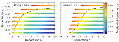
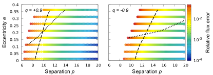
For parameter inference of LISA-type EMRIs, a mode distribution error of is adequate [64, 67]. Inference requirements are far more stringent for the fluxes, but these will not be attained even with ‘exact’ adiabatic models. Comparisons to numerical adiabatic evolutions of equatorial orbits [63] suggest that relative flux errors (of ) will suffice for our waveform to maintain phase coherence with adiabatic LISA-EMRI waveforms over several months; this will also be the level of agreement between adiabatic and post-adiabatic models [149]. We therefore estimate the domain of validity of the PN- results as and across and , excluding the parameter region near the last stable orbit.
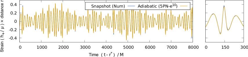
Sample results.—As a concrete example, we present a PN- adiabatic waveform with masses and Kerr spin , initial orbital parameters , and initial phases . We evolve the EMRI over months, starting from the initial apastron with , and ending with final orbital parameter values . During that time the inspiral passes through one strong, : resonance; all other resonances that it encounters are suppressed by additional powers of and and contribute negligible jumps according to Eq. (7).
Figure 3 shows the first hours of the PN- adiabatic strain . For reference, we also plot the snapshot strain from the fixed geodesic source (i.e., without GSF effects) with the same initial frequencies, generated by the BHPC’s numerical Teukolsky solver [57]; this serves as a benchmark for the PN- waveform so long as the viewing time is much shorter than the dephasing time [37, 34], after which the inspiral orbit becomes cycle out of phase with the geodesic orbit. The dephasing time of this sample EMRI is days. As the figure shows, the PN- model faithfully approximates the numerical snapshot, a consequence of the small mode distribution error in the PN- amplitudes.
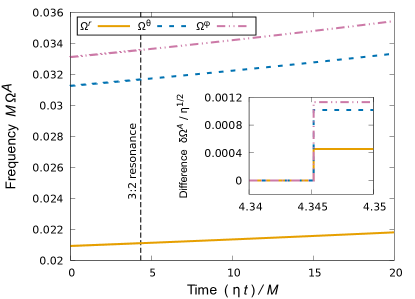
The slow evolution of the adiabatic waveform is more visible in the time-frequency plot 4. The : resonance occurs at , where there are abrupt frequency jumps , corresponding to the jumps estimated from Eq. (7). Although the frequency jumps are small , they lead to large cumulative phase shifts by the termination time . Such shifts are dramatic compared to LISA’s EMRI phase resolution rad [150, 95, 96], reconfirming the importance of GSF resonances for EMRI measurements [92, 93, 94].
Concluding remarks.—Our PN-GSF adiabatic model represents the first user-ready, relativistic description of EMRI waveforms in the astrophysical scenario of generic Kerr orbits, including an approximate treatment of GSF resonances. It can be used to generate on-the-fly waveforms over the whole weak-field, small-eccentricity region of the EMRI parameter space, with arbitrary orbital inclination and Kerr spin, thus opening a new front in ongoing EMRI modelling and data analysis efforts [6, 101].
In the near term, we will improve our PN- analytical calculations to cover more of the EMRI parameter space [143, 70, 151, 152, 153, 154, 155]. We will further accelerate our model towards EMRI data-analysis, using the efficiency-oriented FastEMRIWaveforms framework [100], which will enable a highly parallelized implementation with graphics processing units [64, 67]. Ultimately, we will work on refining the adiabatic model by combining analytical PN-GSF results with numerical GSF data [156, 157, 26, 158, 27, 28, 63, 65, 159, 28, 160, 161, 162], to accomplish a science-adequate, post-adiabatic waveform for LISA.
Finally, it would be informative to compare our adiabatic evolution with small-mass-ratio results from PN theory [163, 164] and fully nonlinear numerical-relativity simulations [165, 166, 167, 168]. This may further delineate the applicable region of GSF theory [169, 40] for generic binary BHs.
Acknowledgements.
Acknowledgments.—We thank Wataru Hikida and Hideyuki Tagoshi for their direct contributions to an earlier version of this manuscript; Scott A. Hughes for helpful discussions on initial phases and comments on the Supplemental Material; Maarten van de Meent for providing independent numerical data to verify BHPC’s Teukolsky results; Leor Barack and Chulmoon Yoo for valuable discussions and comments on the manuscript; and Katsuhiko Ganz, Chris Kavanagh, Koutarou Kyutoku, Yasushi Mino, Takashi Nakamura, Misao Sasaki, Masaru Shibata, and Niels Warburton for very helpful discussions. S.I. is especially grateful to Eric Poisson, Riccardo Sturani and Takahiro Tanaka for their continuous encouragement and insightful discussion about the (adiabatic) evolution scheme for EMRI dynamics. Finally, we thank all the past and present members of the annual Capra meetings with whom we have discussed the techniques and results presented here (over the past decades). S.I. acknowledges support from STFC through grant no. ST/R00045X/1, the GWverse COST Action CA16104,“Black holes, gravitational waves and fundamental physic”, and additional financial support of Ministry of Education - MEC during his stay at IIP-Natal-Brazil. A.J.K.C. acknowledges support from the NASA grants no. 18-LPS18-0027 and 20-LPS20-0005, and from the NSF grant no. PHY-2011968. A.P. acknowledges the support of a Royal Society University Research Fellowship, Research Grant for Research Fellows, Enhancement Awards, and Exchange Grant. This work was supported in part by JSPS/MEXT KAKENHI Grant no. JP16H02183 (R.F.), JP18H04583 (R.F.), JP21H01082 (R.F., H.N. and N.S.), JP17H06358 (H.N. and N.S.), and JP21K03582 (H.N.).References
- Abbott et al. [2019] B. P. Abbott et al. (LIGO Scientific, Virgo), Phys. Rev. X 9, 031040 (2019), arXiv:1811.12907 [astro-ph.HE] .
- Abbott et al. [2021a] R. Abbott et al. (LIGO Scientific, Virgo), Phys. Rev. X 11, 021053 (2021a), arXiv:2010.14527 [gr-qc] .
- Abbott et al. [2021b] R. Abbott et al., arXiv e-prints , arXiv:2108.01045 (2021b), arXiv:2108.01045 [gr-qc] .
- Abbott et al. [2021c] R. Abbott et al., arXiv e-prints , arXiv:2111.03606 (2021c), arXiv:2111.03606 [gr-qc] .
- Amaro-Seoane et al. [2017] P. Amaro-Seoane et al., arXiv e-prints , arXiv:1702.00786 (2017), arXiv:1702.00786 [astro-ph.IM] .
- Kawamura et al. [2021] S. Kawamura et al., PTEP 2021, 05A105 (2021), arXiv:2006.13545 [gr-qc] .
- Mei et al. [2021] J. Mei et al. (TianQin), PTEP 2021, 05A107 (2021), arXiv:2008.10332 [gr-qc] .
- Luo et al. [2021] Z. Luo, Y. Wang, Y. Wu, W. Hu, and G. Jin, PTEP 2021, 05A108 (2021).
- Gong et al. [2021] Y. Gong, J. Luo, and B. Wang, Nature Astron. 5, 881 (2021), arXiv:2109.07442 [astro-ph.IM] .
- Amaro-Seoane [2018] P. Amaro-Seoane, Living Rev. Rel. 21, 4 (2018), arXiv:1205.5240 [astro-ph.CO] .
- Amaro-Seoane [2020] P. Amaro-Seoane, arXiv e-prints , arXiv:2011.03059 (2020), arXiv:2011.03059 [gr-qc] .
- Amaro-Seoane et al. [2007] P. Amaro-Seoane, J. R. Gair, M. Freitag, M. Coleman Miller, I. Mandel, C. J. Cutler, and S. Babak, Class. Quant. Grav. 24, R113 (2007), arXiv:astro-ph/0703495 .
- Babak et al. [2017] S. Babak, J. Gair, A. Sesana, E. Barausse, C. F. Sopuerta, C. P. L. Berry, E. Berti, P. Amaro-Seoane, A. Petiteau, and A. Klein, Phys. Rev. D 95, 103012 (2017), arXiv:1703.09722 [gr-qc] .
- Berry et al. [2019] C. Berry, S. Hughes, C. Sopuerta, A. Chua, A. Heffernan, K. Holley-Bockelmann, D. Mihaylov, C. Miller, and A. Sesana, Bull. Am. Astron. Soc. 51, 42 (2019), arXiv:1903.03686 [astro-ph.HE] .
- Fan et al. [2020] H.-M. Fan, Y.-M. Hu, E. Barausse, A. Sesana, J.-d. Zhang, X. Zhang, T.-G. Zi, and J. Mei, Phys. Rev. D 102, 063016 (2020), arXiv:2005.08212 [astro-ph.HE] .
- Zi et al. [2021] T.-G. Zi, J.-D. Zhang, H.-M. Fan, X.-T. Zhang, Y.-M. Hu, C. Shi, and J. Mei, Phys. Rev. D 104, 064008 (2021), arXiv:2104.06047 [gr-qc] .
- Mino et al. [1997a] Y. Mino, M. Sasaki, and T. Tanaka, Phys. Rev. D 55, 3457 (1997a), arXiv:gr-qc/9606018 .
- Mino et al. [1997b] Y. Mino, M. Sasaki, and T. Tanaka, Prog. Theor. Phys. Suppl. 128, 373 (1997b), arXiv:gr-qc/9712056 .
- Quinn and Wald [1997] T. C. Quinn and R. M. Wald, Phys. Rev. D 56, 3381 (1997), arXiv:gr-qc/9610053 .
- Gralla and Wald [2008] S. E. Gralla and R. M. Wald, Class. Quant. Grav. 25, 205009 (2008), [Erratum: Class.Quant.Grav. 28, 159501 (2011)], arXiv:0806.3293 [gr-qc] .
- Pound [2010] A. Pound, Phys. Rev. D 81, 024023 (2010), arXiv:0907.5197 [gr-qc] .
- Pound [2012] A. Pound, Phys. Rev. Lett. 109, 051101 (2012), arXiv:1201.5089 [gr-qc] .
- Gralla [2012] S. E. Gralla, Phys. Rev. D 85, 124011 (2012), arXiv:1203.3189 [gr-qc] .
- Shah et al. [2012] A. G. Shah, J. L. Friedman, and T. S. Keidl, Phys. Rev. D 86, 084059 (2012), arXiv:1207.5595 [gr-qc] .
- van de Meent [2016] M. van de Meent, Phys. Rev. D 94, 044034 (2016), arXiv:1606.06297 [gr-qc] .
- van de Meent [2018] M. van de Meent, Phys. Rev. D 97, 104033 (2018), arXiv:1711.09607 [gr-qc] .
- Pound et al. [2020] A. Pound, B. Wardell, N. Warburton, and J. Miller, Phys. Rev. Lett. 124, 021101 (2020), arXiv:1908.07419 [gr-qc] .
- Warburton et al. [2021] N. Warburton, A. Pound, B. Wardell, J. Miller, and L. Durkan, Phys. Rev. Lett. 127, 151102 (2021), arXiv:2107.01298 [gr-qc] .
- Mino [2005a] Y. Mino, Class. Quant. Grav. 22, S717 (2005a), arXiv:gr-qc/0506002 .
- Tanaka [2006] T. Tanaka, Prog. Theor. Phys. Suppl. 163, 120 (2006), arXiv:gr-qc/0508114 .
- Barack [2009] L. Barack, Class. Quant. Grav. 26, 213001 (2009), arXiv:0908.1664 [gr-qc] .
- Poisson et al. [2011] E. Poisson, A. Pound, and I. Vega, Living Rev. Rel. 14, 7 (2011), arXiv:1102.0529 [gr-qc] .
- Barack et al. [2019] L. Barack et al., Class. Quant. Grav. 36, 143001 (2019), arXiv:1806.05195 [gr-qc] .
- Barack and Pound [2019] L. Barack and A. Pound, Rept. Prog. Phys. 82, 016904 (2019), arXiv:1805.10385 [gr-qc] .
- [35] Black Hole Perturbation Toolkit, http://bhptoolkit.org/.
- Black Hole Perturbation Club () [B.H.P.C.] Black Hole Perturbation Club (B.H.P.C.), https://sites.google.com/view/bhpc1996/home.
- Detweiler [2005] S. L. Detweiler, Class. Quant. Grav. 22, S681 (2005), arXiv:gr-qc/0501004 .
- Hinderer and Flanagan [2008] T. Hinderer and E. E. Flanagan, Phys. Rev. D 78, 064028 (2008), arXiv:0805.3337 [gr-qc] .
- Miller and Pound [2021] J. Miller and A. Pound, Phys. Rev. D 103, 064048 (2021), arXiv:2006.11263 [gr-qc] .
- van de Meent and Pfeiffer [2020] M. van de Meent and H. P. Pfeiffer, Phys. Rev. Lett. 125, 181101 (2020), arXiv:2006.12036 [gr-qc] .
- Pound and Wardell [2021] A. Pound and B. Wardell, arXiv e-prints , arXiv:2101.04592 (2021), arXiv:2101.04592 [gr-qc] .
- Wardell et al. [2021] B. Wardell, A. Pound, N. Warburton, J. Miller, L. Durkan, and A. Le Tiec, arXiv e-prints , arXiv:2112.12265 (2021), arXiv:2112.12265 [gr-qc] .
- Hughes [2000] S. A. Hughes, Phys. Rev. D 61, 084004 (2000), [Erratum: Phys. Rev. D 63, 049902 (2001), Erratum: Phys. Rev. D 65, 069902 (2002), Erratum: Phys. Rev. D 67, 089901 (2003), Erratum: Phys. Rev. D 78, 109902 (2008), Erratum: Phys. Rev. D 90, 109904 (2014)], arXiv:gr-qc/9910091 .
- Mino [2003] Y. Mino, Phys. Rev. D 67, 084027 (2003), arXiv:gr-qc/0302075 .
- Hughes et al. [2005] S. A. Hughes, S. Drasco, E. E. Flanagan, and J. Franklin, Phys. Rev. Lett. 94, 221101 (2005), arXiv:gr-qc/0504015 .
- Mino [2005b] Y. Mino, Prog. Theor. Phys. 113, 733 (2005b), arXiv:gr-qc/0506003 .
- Mino [2006] Y. Mino, Prog. Theor. Phys. 115, 43 (2006), arXiv:gr-qc/0601019 .
- Mino [2008] Y. Mino, Phys. Rev. D 77, 044008 (2008), arXiv:0711.3007 [gr-qc] .
- Nakamura et al. [1987] T. Nakamura, K. Oohara, and Y. Kojima, Prog. Theor. Phys. Suppl. 90, 1 (1987).
- Finn and Thorne [2000] L. S. Finn and K. S. Thorne, Phys. Rev. D 62, 124021 (2000), arXiv:gr-qc/0007074 .
- Glampedakis and Kennefick [2002] K. Glampedakis and D. Kennefick, Phys. Rev. D 66, 044002 (2002), arXiv:gr-qc/0203086 .
- Hughes [2001] S. A. Hughes, Phys. Rev. D 64, 064004 (2001), [Erratum: Phys.Rev.D 88, 109902 (2013)], arXiv:gr-qc/0104041 .
- Fujita and Tagoshi [2004] R. Fujita and H. Tagoshi, Prog. Theor. Phys. 112, 415 (2004), arXiv:gr-qc/0410018 .
- Drasco and Hughes [2006] S. Drasco and S. A. Hughes, Phys. Rev. D 73, 024027 (2006), [Erratum: Phys. Rev. D 88, 109905 (2013), Erratum: Phys. Rev. D 90, 109905 (2014)], arXiv:gr-qc/0509101 .
- Sundararajan et al. [2007] P. A. Sundararajan, G. Khanna, and S. A. Hughes, Phys. Rev. D 76, 104005 (2007), arXiv:gr-qc/0703028 .
- Sundararajan et al. [2008] P. A. Sundararajan, G. Khanna, S. A. Hughes, and S. Drasco, Phys. Rev. D 78, 024022 (2008), arXiv:0803.0317 [gr-qc] .
- Fujita et al. [2009] R. Fujita, W. Hikida, and H. Tagoshi, Prog. Theor. Phys. 121, 843 (2009), arXiv:0904.3810 [gr-qc] .
- Harms et al. [2013] E. Harms, S. Bernuzzi, and B. Brügmann, Class. Quant. Grav. 30, 115013 (2013), arXiv:1301.1591 [gr-qc] .
- Harms et al. [2014] E. Harms, S. Bernuzzi, A. Nagar, and A. Zenginoglu, Class. Quant. Grav. 31, 245004 (2014), arXiv:1406.5983 [gr-qc] .
- Gralla et al. [2016] S. E. Gralla, S. A. Hughes, and N. Warburton, Class. Quant. Grav. 33, 155002 (2016), [Erratum: Class.Quant.Grav. 37, 109501 (2020)], arXiv:1603.01221 [gr-qc] .
- Burke et al. [2020] O. Burke, J. R. Gair, and J. Simón, Phys. Rev. D 101, 064026 (2020), arXiv:1909.12846 [gr-qc] .
- Gourgoulhon et al. [2019] E. Gourgoulhon, A. Le Tiec, F. H. Vincent, and N. Warburton, Astron. Astrophys. 627, A92 (2019), arXiv:1903.02049 [gr-qc] .
- Fujita and Shibata [2020] R. Fujita and M. Shibata, Phys. Rev. D 102, 064005 (2020), arXiv:2008.13554 [gr-qc] .
- Chua et al. [2021] A. J. K. Chua, M. L. Katz, N. Warburton, and S. A. Hughes, Phys. Rev. Lett. 126, 051102 (2021), arXiv:2008.06071 [gr-qc] .
- Hughes et al. [2021] S. A. Hughes, N. Warburton, G. Khanna, A. J. K. Chua, and M. L. Katz, Phys. Rev. D 103, 104014 (2021), arXiv:2102.02713 [gr-qc] .
- Barton et al. [2008] J. L. Barton, D. J. Lazar, D. J. Kennefick, G. Khanna, and L. M. Burko, Phys. Rev. D 78, 064042 (2008), arXiv:0804.1075 [gr-qc] .
- Katz et al. [2021] M. L. Katz, A. J. K. Chua, L. Speri, N. Warburton, and S. A. Hughes, Phys. Rev. D 104, 064047 (2021), arXiv:2104.04582 [gr-qc] .
- Mino et al. [1997c] Y. Mino, M. Sasaki, M. Shibata, H. Tagoshi, and T. Tanaka, Prog. Theor. Phys. Suppl. 128, 1 (1997c), arXiv:gr-qc/9712057 .
- Sasaki and Tagoshi [2003] M. Sasaki and H. Tagoshi, Living Rev. Rel. 6, 6 (2003), arXiv:gr-qc/0306120 .
- Fujita [2015] R. Fujita, PTEP 2015, 033E01 (2015), arXiv:1412.5689 [gr-qc] .
- Sago and Fujita [2015] N. Sago and R. Fujita, PTEP 2015, 073E03 (2015), arXiv:1505.01600 [gr-qc] .
- Kavanagh et al. [2016] C. Kavanagh, A. C. Ottewill, and B. Wardell, Phys. Rev. D 93, 124038 (2016), arXiv:1601.03394 [gr-qc] .
- Bini and Geralico [2018] D. Bini and A. Geralico, Found. Phys. 48, 1349 (2018).
- Bini and Geralico [2019] D. Bini and A. Geralico, Phys. Rev. D 100, 104002 (2019), arXiv:1907.11080 [gr-qc] .
- Munna [2020a] C. Munna, , Ph.D. thesis, North Carolina U. (2020a).
- Yunes et al. [2010] N. Yunes, A. Buonanno, S. A. Hughes, M. Coleman Miller, and Y. Pan, Phys. Rev. Lett. 104, 091102 (2010), arXiv:0909.4263 [gr-qc] .
- Yunes et al. [2011] N. Yunes, A. Buonanno, S. A. Hughes, Y. Pan, E. Barausse, M. Miller, and W. Throwe, Phys. Rev. D 83, 044044 (2011), [Erratum: Phys. Rev. D 88, 109904 (2013)], arXiv:1009.6013 [gr-qc] .
- Xin et al. [2019] S. Xin, W.-B. Han, and S.-C. Yang, Phys. Rev. D 100, 084055 (2019), arXiv:1812.04185 [gr-qc] .
- Zhang et al. [2021] C. Zhang, W.-B. Han, X.-Y. Zhong, and G. Wang, Phys. Rev. D 104, 024050 (2021), arXiv:2102.05391 [gr-qc] .
- Albanesi et al. [2021] S. Albanesi, A. Nagar, and S. Bernuzzi, Phys. Rev. D 104, 024067 (2021), arXiv:2104.10559 [gr-qc] .
- Glampedakis et al. [2002] K. Glampedakis, S. A. Hughes, and D. Kennefick, Phys. Rev. D 66, 064005 (2002), arXiv:gr-qc/0205033 .
- Barack and Cutler [2004] L. Barack and C. Cutler, Phys. Rev. D 69, 082005 (2004), arXiv:gr-qc/0310125 .
- Gair and Glampedakis [2006] J. R. Gair and K. Glampedakis, Phys. Rev. D 73, 064037 (2006), arXiv:gr-qc/0510129 .
- Babak et al. [2007] S. Babak, H. Fang, J. R. Gair, K. Glampedakis, and S. A. Hughes, Phys. Rev. D 75, 024005 (2007), [Erratum: Phys. Rev. D 77, 04990 (2008)], arXiv:gr-qc/0607007 .
- Sopuerta and Yunes [2011] C. F. Sopuerta and N. Yunes, Phys. Rev. D 84, 124060 (2011), arXiv:1109.0572 [gr-qc] .
- Chua and Gair [2015] A. J. Chua and J. R. Gair, Class. Quant. Grav. 32, 232002 (2015), arXiv:1510.06245 [gr-qc] .
- Chua et al. [2017] A. J. Chua, C. J. Moore, and J. R. Gair, Phys. Rev. D 96, 044005 (2017), arXiv:1705.04259 [gr-qc] .
- Apostolatos et al. [2009] T. A. Apostolatos, G. Lukes-Gerakopoulos, and G. Contopoulos, Phys. Rev. Lett. 103, 111101 (2009), arXiv:0906.0093 [gr-qc] .
- Flanagan and Hinderer [2012] E. E. Flanagan and T. Hinderer, Phys. Rev. Lett. 109, 071102 (2012), arXiv:1009.4923 [gr-qc] .
- Brink et al. [2015a] J. Brink, M. Geyer, and T. Hinderer, Phys. Rev. Lett. 114, 081102 (2015a), arXiv:1304.0330 [gr-qc] .
- Brink et al. [2015b] J. Brink, M. Geyer, and T. Hinderer, Phys. Rev. D 91, 083001 (2015b), arXiv:1501.07728 [gr-qc] .
- Ruangsri and Hughes [2014] U. Ruangsri and S. A. Hughes, Phys. Rev. D 89, 084036 (2014), arXiv:1307.6483 [gr-qc] .
- Berry et al. [2016] C. P. L. Berry, R. H. Cole, P. Cañizares, and J. R. Gair, Phys. Rev. D 94, 124042 (2016), arXiv:1608.08951 [gr-qc] .
- Speri and Gair [2021] L. Speri and J. R. Gair, Phys. Rev. D 103, 124032 (2021), arXiv:2103.06306 [gr-qc] .
- Bonga et al. [2019] B. Bonga, H. Yang, and S. A. Hughes, Phys. Rev. Lett. 123, 101103 (2019), arXiv:1905.00030 [gr-qc] .
- Gupta et al. [2021] P. Gupta, B. Bonga, A. J. K. Chua, and T. Tanaka, Phys. Rev. D 104, 044056 (2021), arXiv:2104.03422 [gr-qc] .
- Coogan et al. [2022] A. Coogan, G. Bertone, D. Gaggero, B. J. Kavanagh, and D. A. Nichols, Phys. Rev. D 105, 043009 (2022), arXiv:2108.04154 [gr-qc] .
- Barsanti et al. [2022] S. Barsanti, N. Franchini, L. Gualtieri, A. Maselli, and T. P. Sotiriou, arXiv e-prints , arXiv:2203.05003 (2022), arXiv:2203.05003 [gr-qc] .
- [99] EMRI Kludge Suite, https://github.com/alvincjk/EMRI_Kludge_Suite/.
- [100] few: Fast EMRI Waveforms, https://bhptoolkit.org/FastEMRIWaveforms/html/index.html.
- Chua and Cutler [2021] A. J. K. Chua and C. J. Cutler, arXiv e-prints , arXiv:2109.14254 (2021), arXiv:2109.14254 [gr-qc] .
- [102] LISA Data Challenges, https://lisa-ldc.lal.in2p3.fr/.
- Pan et al. [2011] Y. Pan, A. Buonanno, R. Fujita, E. Racine, and H. Tagoshi, Phys. Rev. D 83, 064003 (2011), [Erratum: Phys. Rev. D 87, 109901 (2013)], arXiv:1006.0431 [gr-qc] .
- Pratten et al. [2020] G. Pratten, S. Husa, C. Garcia-Quiros, M. Colleoni, A. Ramos-Buades, H. Estelles, and R. Jaume, Phys. Rev. D 102, 064001 (2020), arXiv:2001.11412 [gr-qc] .
- Rifat et al. [2020] N. E. M. Rifat, S. E. Field, G. Khanna, and V. Varma, Phys. Rev. D 101, 081502 (2020), arXiv:1910.10473 [gr-qc] .
- Islam et al. [2022] T. Islam, S. E. Field, S. A. Hughes, G. Khanna, V. Varma, M. Giesler, M. A. Scheel, L. E. Kidder, and H. P. Pfeiffer, arXiv e-prints , arXiv:2204.01972 (2022), arXiv:2204.01972 [gr-qc] .
- Ajith et al. [2008] P. Ajith et al., Phys. Rev. D 77, 104017 (2008), [Erratum: Phys.Rev.D 79, 129901 (2009)], arXiv:0710.2335 [gr-qc] .
- Aylott et al. [2009] B. Aylott et al., Class. Quant. Grav. 26, 165008 (2009), arXiv:0901.4399 [gr-qc] .
- Ajith et al. [2012] P. Ajith et al., Class. Quant. Grav. 29, 124001 (2012), [Erratum: Class. Quant. Grav. 30, 199401 (2013)], arXiv:1201.5319 [gr-qc] .
- Hinder et al. [2014] I. Hinder et al., Class. Quant. Grav. 31, 025012 (2014), arXiv:1307.5307 [gr-qc] .
- Sago et al. [2005] N. Sago, T. Tanaka, W. Hikida, and H. Nakano, Prog. Theor. Phys. 114, 509 (2005), arXiv:gr-qc/0506092 .
- Cutler et al. [1994] C. Cutler, D. Kennefick, and E. Poisson, Phys. Rev. D 50, 3816 (1994).
- Schmidt [2002] W. Schmidt, Class. Quant. Grav. 19, 2743 (2002), arXiv:gr-qc/0202090 .
- Carter [1968] B. Carter, Phys. Rev. 174, 1559 (1968).
- Teukolsky [1972] S. Teukolsky, Phys. Rev. Lett. 29, 1114 (1972).
- Teukolsky [1973] S. A. Teukolsky, Astrophys. J. 185, 635 (1973).
- Teukolsky and Press [1974] S. Teukolsky and W. Press, Astrophys. J. 193, 443 (1974).
- See Supplemental Material at [2021a] See Supplemental Material at, [URL will be inserted by publisher] (2021a), for a comparison with another adiabatic-evolution scheme in Ref. [65].
- Sago et al. [2006] N. Sago, T. Tanaka, W. Hikida, K. Ganz, and H. Nakano, Prog. Theor. Phys. 115, 873 (2006), arXiv:gr-qc/0511151 .
- Drasco et al. [2005] S. Drasco, E. E. Flanagan, and S. A. Hughes, Class. Quant. Grav. 22, S801 (2005), arXiv:gr-qc/0505075 .
- Isoyama et al. [2019] S. Isoyama, R. Fujita, H. Nakano, N. Sago, and T. Tanaka, PTEP 2019, 013E01 (2019), arXiv:1809.11118 [gr-qc] .
- Gair et al. [2012] J. Gair, N. Yunes, and C. M. Bender, J. Math. Phys. 53, 032503 (2012), arXiv:1111.3605 [gr-qc] .
- Grossman et al. [2013] R. Grossman, J. Levin, and G. Perez-Giz, Phys. Rev. D 88, 023002 (2013), arXiv:1108.1819 [gr-qc] .
- Flanagan et al. [2014] E. E. Flanagan, S. A. Hughes, and U. Ruangsri, Phys. Rev. D 89, 084028 (2014), arXiv:1208.3906 [gr-qc] .
- Isoyama et al. [2013] S. Isoyama, R. Fujita, H. Nakano, N. Sago, and T. Tanaka, PTEP 2013, 063E01 (2013), arXiv:1302.4035 [gr-qc] .
- van de Meent [2014] M. van de Meent, Phys. Rev. D 89, 084033 (2014), arXiv:1311.4457 [gr-qc] .
- Mihaylov and Gair [2017] D. P. Mihaylov and J. R. Gair, J. Math. Phys. 58, 112501 (2017), arXiv:1706.06639 [gr-qc] .
- Lukes-Gerakopoulos and Witzany [2020] G. Lukes-Gerakopoulos and V. Witzany, Nonlinear effects in emri dynamics and their imprints on gravitational waves, in Handbook of Gravitational Wave Astronomy, edited by C. Bambi, S. Katsanevas, and K. D. Kokkotas (Springer Singapore, Singapore, 2020) pp. 1–44.
- Fujita et al. [2017] R. Fujita, S. Isoyama, A. Le Tiec, H. Nakano, N. Sago, and T. Tanaka, Class. Quant. Grav. 34, 134001 (2017), arXiv:1612.02504 [gr-qc] .
- See Supplemental Material at [2021b] See Supplemental Material at, [URL will be inserted by publisher] (2021b), for a sketch of the derivation of Eq. (8).
- Nasipak and Evans [2021] Z. Nasipak and C. R. Evans, Phys. Rev. D 104, 084011 (2021), arXiv:2105.15188 [gr-qc] .
- Fujita and Hikida [2009] R. Fujita and W. Hikida, Class. Quant. Grav. 26, 135002 (2009), arXiv:0906.1420 [gr-qc] .
- Fackerell and Crossman [1977] E. D. Fackerell and R. G. Crossman, Journal of Mathematical Physics 18, 1849 (1977).
- Mano et al. [1996] S. Mano, H. Suzuki, and E. Takasugi, Prog. Theor. Phys. 95, 1079 (1996), arXiv:gr-qc/9603020 .
- Mano and Takasugi [1997] S. Mano and E. Takasugi, Prog. Theor. Phys. 97, 213 (1997), arXiv:gr-qc/9611014 .
- Shibata et al. [1995] M. Shibata, M. Sasaki, H. Tagoshi, and T. Tanaka, Phys. Rev. D 51, 1646 (1995), arXiv:gr-qc/9409054 .
- Tagoshi [1995] H. Tagoshi, Prog. Theor. Phys. 93, 307 (1995), [Erratum: Prog. Theor. Phys. 118, 577–579 (2007)].
- Tagoshi et al. [1996] H. Tagoshi, M. Shibata, T. Tanaka, and M. Sasaki, Phys. Rev. D 54, 1439 (1996), arXiv:gr-qc/9603028 .
- Tanaka et al. [1996] T. Tanaka, H. Tagoshi, and M. Sasaki, Prog. Theor. Phys. 96, 1087 (1996), arXiv:gr-qc/9701050 .
- Tagoshi et al. [1997] H. Tagoshi, S. Mano, and E. Takasugi, Prog. Theor. Phys. 98, 829 (1997), arXiv:gr-qc/9711072 .
- Ganz et al. [2007] K. Ganz, W. Hikida, H. Nakano, N. Sago, and T. Tanaka, Prog. Theor. Phys. 117, 1041 (2007), arXiv:gr-qc/0702054 .
- Fujita [2012a] R. Fujita, Prog. Theor. Phys. 127, 583 (2012a), arXiv:1104.5615 [gr-qc] .
- Fujita [2012b] R. Fujita, Prog. Theor. Phys. 128, 971 (2012b), arXiv:1211.5535 [gr-qc] .
- The PN- results for the spheroidal harmonics , Teukolsky amplitudes , and fluxes used in this work are all available for download at [2021] The PN- results for the spheroidal harmonics , Teukolsky amplitudes , and fluxes used in this work are all available for download at, [https://sites.google.com/view/bhpc1996/data] (2021).
- Nasipak et al. [2019] Z. Nasipak, T. Osburn, and C. R. Evans, Phys. Rev. D 100, 064008 (2019), arXiv:1905.13237 [gr-qc] .
- Fujita and Tagoshi [2005] R. Fujita and H. Tagoshi, Prog. Theor. Phys. 113, 1165 (2005), arXiv:0904.3818 [gr-qc] .
- See Supplemental Material at [2021c] See Supplemental Material at, [URL will be inserted by publisher] (2021c), for additional plots of relative flux errors.
- Stein and Warburton [2020] L. C. Stein and N. Warburton, Phys. Rev. D 101, 064007 (2020), arXiv:1912.07609 [gr-qc] .
- See Supplemental Material at [2021d] See Supplemental Material at, [URL will be inserted by publisher] (2021d), which includes Refs. [170, 171, 172, 173], for an estimate of the dephasing between adiabatic and first post-adiabatic model.
- Lindblom et al. [2008] L. Lindblom, B. J. Owen, and D. A. Brown, Phys. Rev. D 78, 124020 (2008), arXiv:0809.3844 [gr-qc] .
- Shah [2014] A. G. Shah, Phys. Rev. D 90, 044025 (2014), arXiv:1403.2697 [gr-qc] .
- Munna and Evans [2019] C. Munna and C. R. Evans, Phys. Rev. D 100, 104060 (2019), arXiv:1909.05877 [gr-qc] .
- Munna et al. [2020] C. Munna, C. R. Evans, S. Hopper, and E. Forseth, Phys. Rev. D 102, 024047 (2020), arXiv:2005.03044 [gr-qc] .
- Munna [2020b] C. Munna, Phys. Rev. D 102, 124001 (2020b), arXiv:2008.10622 [gr-qc] .
- Munna and Evans [2020] C. Munna and C. R. Evans, Phys. Rev. D 102, 104006 (2020), arXiv:2009.01254 [gr-qc] .
- Warburton et al. [2012] N. Warburton, S. Akcay, L. Barack, J. R. Gair, and N. Sago, Phys. Rev. D 85, 061501 (2012), arXiv:1111.6908 [gr-qc] .
- Osburn et al. [2016] T. Osburn, N. Warburton, and C. R. Evans, Phys. Rev. D 93, 064024 (2016), arXiv:1511.01498 [gr-qc] .
- Van De Meent and Warburton [2018] M. Van De Meent and N. Warburton, Class. Quant. Grav. 35, 144003 (2018), arXiv:1802.05281 [gr-qc] .
- McCart et al. [2021] J. McCart, T. Osburn, and J. Y. J. Burton, Phys. Rev. D 104, 084050 (2021), arXiv:2109.00056 [gr-qc] .
- Lynch et al. [2021] P. Lynch, M. van de Meent, and N. Warburton, arXiv e-prints , arXiv:2112.05651 (2021), arXiv:2112.05651 [gr-qc] .
- Mathews et al. [2022] J. Mathews, A. Pound, and B. Wardell, Phys. Rev. D 105, 084031 (2022), arXiv:2112.13069 [gr-qc] .
- Skoupý and Lukes-Gerakopoulos [2022] V. Skoupý and G. Lukes-Gerakopoulos, Phys. Rev. D 105, 084033 (2022), arXiv:2201.07044 [gr-qc] .
- Will and Maitra [2017] C. M. Will and M. Maitra, Phys. Rev. D 95, 064003 (2017), arXiv:1611.06931 [gr-qc] .
- Tucker and Will [2021] A. Tucker and C. M. Will, Phys. Rev. D 104, 104023 (2021), arXiv:2108.12210 [gr-qc] .
- Lewis et al. [2017] A. G. M. Lewis, A. Zimmerman, and H. P. Pfeiffer, Class. Quant. Grav. 34, 124001 (2017), arXiv:1611.03418 [gr-qc] .
- Fernando et al. [2019] M. Fernando, D. Neilsen, H. Lim, E. Hirschmann, and H. Sundar, SIAM J. Sci. Comput. 41, C97 (2019), arXiv:1807.06128 [gr-qc] .
- Lousto and Healy [2020] C. O. Lousto and J. Healy, Phys. Rev. Lett. 125, 191102 (2020), arXiv:2006.04818 [gr-qc] .
- Lousto and Healy [2022] C. O. Lousto and J. Healy, arXiv e-prints , arXiv:2203.08831 (2022), arXiv:2203.08831 [gr-qc] .
- Le Tiec [2014] A. Le Tiec, Int. J. Mod. Phys. D 23, 1430022 (2014), arXiv:1408.5505 [gr-qc] .
- Barack and Sago [2009] L. Barack and N. Sago, Phys. Rev. Lett. 102, 191101 (2009), arXiv:0902.0573 [gr-qc] .
- Le Tiec et al. [2012] A. Le Tiec, E. Barausse, and A. Buonanno, Phys. Rev. Lett. 108, 131103 (2012), arXiv:1111.5609 [gr-qc] .
- Isoyama et al. [2014] S. Isoyama, L. Barack, S. R. Dolan, A. Le Tiec, H. Nakano, A. G. Shah, T. Tanaka, and N. Warburton, Phys. Rev. Lett. 113, 161101 (2014), arXiv:1404.6133 [gr-qc] .
- van de Meent [2017] M. van de Meent, Phys. Rev. Lett. 118, 011101 (2017), arXiv:1610.03497 [gr-qc] .