Abstract

We show how a modified Friedmann equation, originating from a model of the universe built from a certain $W_{3}$ algebra, has the potential to explain the difference between the Hubble constants extracted from CMB data and from supernova data.

1 Introduction

The model of our Universe introduced in [1] is an attempt to explain how time and space emerged in our present universe, starting from a string field theory based on a certain $W_{3}$ algebra. It led in addition (under certain natural assumptions) to a modified Friedmann equation [2]. An appealing feature of this Friedmann equation is that it needs no cosmological term, but that it nevertheless results in an exponentially expanding universe at late times and that this exponential expansion is linked to the creation of baby universes and wormholes in the quantum universe. In this way the quantum aspects of gravity at the smallest distances become linked to the largest distances of our classical universe. We refer to [1] for a detailed discussion of these aspects, but let us for the convenience of the reader just outline the general picture emerging from [1]: by a breaking of the mentioned $W_{3}$ symmetry, universes can be created. They have both cosmological constants and a new constant related to the creation of baby universes. It is dominantly two-dimensional universes with different “flavors” (coming from the $W_{3}$ algebra) which expand and they might expand very fast (faster than exponentially) to macroscopic scales. During this expansion the interaction between universes with different flavors turns these two-dimensional universes into a higher dimensional universe, the dimension of which is determined by the symmetry breaking of the $W_{3}$ algebra. Possible dimensions of the resulting spacetime are 3, 4, 6 and 10. The expansion triggered by the cosmological constant is then stopped because the Coleman mechanism is operating, and we imagine that it will also be operating at all later times. The appearance of dimensions 3, 4, 6 and 10 is of course tantalizing and suggests the possibility that our model could be equivalent to a superstring theory where all matter fields are integrated out.

The purpose of this article is to show that without further assumptions than already present in [2] our modified Friedmann equation can explain why one obtains different values for the Hubble constant $H_{0}$ when using CMB data [3] and supernova data [4]. Before doing that, in order to avoid misunderstanding, let us clarify which cosmological problems we do not address, namely the hierarchy problem and the naturalness problem, and what problem we do address, namely the $H_{0}$ problem.

The hierarchy problem is that the observed value of dark energy is much too small compared to the Planck scale which will appear in any calculation involving quantum field theory interacting with gravity. We will assume that this problem has been solved by the Coleman mechanism and that the value of dark energy we observe today comes entirely from our new parameter $B$. This parameter is not influenced by the Coleman mechanism, but we will not here try to explain its actual value. In principle it might be possible since it is related to the creation of baby universes in our “real” theory based on $W_{3}$ algebra, which underlies our modified Friedmann equation. However, presently we are not able to follow the renormalization flow of this coupling constant from the creation of our universe to present time. Thus we cannot explain the “smallness” of our parameter $B$, just like the smallness of $\Lambda$ cannot be explained from first principles in the standard $\Lambda$CMD cosmology.

The naturalness problem is that after symmetry breaking of any kind, whether it is at electroweak scale or QCD scale or any similar scale, the contribution to dark energy will be very large compared to the present small value and some unknown fine tuning has to take place to accommodate the present observed value of dark energy. We do not try to solve this problem, but again simply assume that the Coleman mechanism is operating and the cosmological constant coming from such contributions can be set to zero. Since our model provides us with a new mechanism for the expansion of the universe at late time, we do not need a non-zero cosmological constant.

A third cosmological problem is the $H_{0}$ problem: if one believes in the direct, local observation of $H_{0}$, which is obtained by the cosmic ladder of Cepheid-SNIa standard candles, it differs by $5\,\sigma$ from the estimated $H_{0}$ value obtained from the CMB data, obtained by using the $\Lambda$CDM model to extrapolate from the time of last scattering to present days time. This is the problem to which our model provides a solution, since our modified Friedmann equation leads to a different extrapolation from the time of last scattering to present days time than provided by the $\Lambda$CDM model.

2 The modified Friedmann equation

The (first) Friedmann equation is

$$\left(\frac{\dot{a}}{a}\right)^{2}=\frac{\kappa\rho+\Lambda}{3},\qquad\dot{a}:=\frac{da(t)}{dt},$$ (1)

where $\kappa=8\pi G$ and where $G$ and $\Lambda$ denote the gravitational and the cosmological constants. $a(t)$ denotes the scale factor in a universe assumed homogeneous and isotropic with matter density $\rho$ and we have assumed the spatial curvature is zero, i.e. $\Omega_{\rm K}=0$. In [2] we showed that our modified Friedmann equation is

$$\left(\frac{\dot{a}}{a}\right)^{2}=\frac{\kappa\rho}{3}+\frac{Ba}{\dot{a}}\frac{(1+3F(x))}{F^{2}(x)},\quad x:=\frac{Ba^{3}}{\dot{a}^{3}},\quad F^{2}(x)-F^{3}(x)=x.$$ (2)

In eq. (2) we have assumed that $\Lambda=0$, in accordance with our above mentioned assumption that the Coleman mechanism is operative. Further, we argued in [1, 2] that the space topology should be toroidal, and thus that the spatial curvature term $\Omega_{\rm K}=0$. A new coupling constant, denoted $B$, is present in our modified Friedmann equation. It is proportional to the coupling constant which in our underlying string field theory model describes the creation of baby universes and wormholes. At late times the $B$-term acts effectively as a cosmological term and one can show that

$$a(t)\;\propto\;{\rm e}^{(27B/4)^{1/3}t}\quad{\rm for}\quad t\to\infty.$$ (3)

Assuming a simple matter dust system, such that the pressure $p=0$, we can write

$$\kappa\rho=\frac{C}{a^{3}},$$ (4)

where $C$ is a positive constant.

We can now solve (2) numerically assuming that $a(t)\!=\!0$ at $t\!=\!0$, which we define as the time of the Big Bang. This will determine $a(t)$ up to a constant of proportionality, and the solution will be parametrized by $B$. One has an expansion of $a(t)$ in powers of $Bt^{3}$:

$$a_{B}(t) = \alpha\,t^{2/3}\left(1+\frac{9}{8}\,Bt^{3}+O\Big{(}(Bt^{3})^{2}\Big{)}\right)$$ (5)

$$\dot{a}_{B}(t) = \alpha\,t^{-1/3}\left(\frac{2}{3}+\frac{33}{8}\,Bt^{3}+O\Big{(}(Bt^{3})^{2}\Big{)}\right)$$ (6)

$$\ddot{a}_{B}(t) = \alpha\,t^{-4/3}\left(-\frac{2}{9}+11\,Bt^{3}+O\Big{(}(Bt^{3})^{2}\Big{)}\right)$$ (7)

In particular we find that the Hubble parameter has the expansion

$$H_{B}(t):=\frac{\dot{a}_{B}}{a_{B}}=\frac{2}{3t}\left(1+\frac{81}{16}Bt^{3}+O\Big{(}(Bt^{3})^{2}\Big{)}\right)$$ (8)

and that the time $t_{*}$ where the acceleration of the universe starts, defined as the zero of $\ddot{a}(t)/a(t)$, is determined by

$$\frac{\ddot{a}_{B}(t_{*})}{a_{B}(t_{*})}=-\frac{2}{9t_{*}^{2}}\left(1-\frac{405}{8}\,Bt^{3}_{*}+O\Big{(}(Bt^{3}_{*})^{2}\Big{)}\right)=0$$ (9)

Of course we do not expect the matter dust approximation (4) to be good for small $t$. At some point it has to be replaced by the radiation dominated equation of state and for even smaller $t$ some kind of inflationary scenario should presumably take place. In particular, when the universe approaches the Planck size one will have to address the underlying quantum theory of gravity. Our model based on a certain $W_{3}$ algebra is an attempt to deal with issues at this small scale, but it also led to the modified Friedmann equation (2) which should be valid only when the universe is of macroscopic size. In the following we will only apply it at times equal or larger than the time $t_{\rm LS}$ of last scattering of the CMB, which is well beyond the time when the matter dominated era starts.

3 From CMB H₀ to standard candle H₀

Let us compare eq. (8) with the corresponding equation using the standard Friedmann equation (1). In that case we obtain

$$H_{\Lambda}(t)=\frac{2}{3t}\,\left(1+\frac{1}{4}\Lambda t^{2}+O\Big{(}(\Lambda t^{2})^{2}\Big{)}\right)$$ (10)

As indicated by the expansions (8) and (10) the fall-off of $H_{B}(t)$ with time $t$ is slower than that of $H_{\Lambda}(t)$. The measurement of $H(t)$ using CMB refers to $H_{\Lambda}(t)$ at the time of last scattering $t_{\rm LS}^{\rm CMB}$, extrapolated to the present time $t_{0}^{\rm CMB}$ using the $\Lambda$CDM model. This leads to $H_{\Lambda^{\rm CMB}}(t_{0}^{\rm CMB}):=H^{\rm CMB}_{0}$ [3]:

$$67.27-0.60<H^{\rm CMB}_{0}<67.27+0.60,\qquad t_{0}^{\rm CMB}=13.8\times 10^{9}\,{\rm y}.$$ (11)

On the other hand the data from standard candles (SC) such as Type Ia supernovae and gamma-ray bursts [4] are measuring $H(t)$ with $t$ approximately equal to the present time and the result is

$$73.20-1.30<H^{\rm SC}_{0}<73.20+1.30.$$ (12)

The redshift is defined as

$$z(t):=\frac{a(t_{0})}{a(t)}-1,$$ (13)

where $t_{0}$ denotes the present time. Two of the simplest observables we have at our disposal are the measured temperature of the CMB, $T^{\rm CMB}$, and the measured Hubble constant, i.e. $H^{\rm SC}_{0}$. We assume that the measured temperature $T^{\rm CMB}=T(t_{0})$ at the present time $t_{0}$ originates from the temperature at last scattering, $T(t_{\rm LS})$ cooled down by the expansion of the universe. The time of last scattering is so early in the history of the universe that we will ignore the dependence of $t_{\rm LS}$ on parameters $\Lambda$ in the $\Lambda$CDM model and $B$ in our model, i.e. we assume $t_{\rm LS}^{\rm CMB}=t_{\rm LS}^{\rm B}~{}(=t_{\rm LS})$. Finally, the fact that CMB spectrum is a black-body spectrum implies that the scale factor $a(t)\propto 1/T(t)$ for $t$ larger than $t_{\rm LS}$. We know $T(t_{\rm LS})$ to good precision for physical reasons not related to any specific cosmological model. Thus a determination of the CMB temperature $T^{\rm CMB}$ is also a determination of $a(t_{0})/a(t_{\rm LS})$ and therefore of the redshift $z(t_{\rm LS})$. The measurement of the CMB temperature leads to $z(t_{\rm LS})=1090$. We have redshifts $z_{B}(t)$ and $z_{\Lambda}(t)$ which depend on the parameters $B$ and $\Lambda$ for our model and the $\Lambda$CDM model, respectively. We now determine the parameters $B$ and the present time $t_{0}^{\rm B}$ for our model by requiring that

$$z_{\rm B}(t_{\rm LS})=1090\quad\big{(}=z_{\Lambda}(t_{\rm LS})\big{)}$$ (14)

and

$$H_{B}(t_{0}^{\rm B})=H^{\rm SC}_{0}.$$ (15)

We obtain

$$\big{(}t_{0}^{\rm B}\big{)}^{3}B=0.1500\pm 0.0056,\qquad t_{0}^{\rm B}=13.882\pm 0.043\;[{\rm Gyr}].$$ (16)

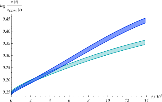
Figure 1: The green region is $\log z_{\Lambda}(t)/z_{\rm CDM}(t)$ of the $\Lambda$CDM model, with the values of $H_{0}^{\rm CMB}$, $\Lambda^{\rm CMB}$ and $t_{0}^{\rm CMB}$ taken from [3]. The blue lines define the region for $\log z_{B}(t)/z_{\rm CDM}(t)$ of our model, where $B$ iand $t_{0}^{\rm B}$ are determined as described in the main text. Note that $t_{\rm LS}$ cannot be distinguished from $t=0$ on the figure. Similarly $t_{0}^{\rm CMB}$ cannot be distinguished from $t_{0}^{\rm B}$.

We have illustrated the situation in Fig. 1. Defining $z_{\rm CDM}(t):=z_{\Lambda=0}(t)=z_{{\rm B}=0}(t)$, a convenient variable is $\log\big{[}z(t)/z_{\rm CDM}(t)\big{]}$ and we can now plot this variable for the $\Lambda$CDM model for the CMB values of $H^{\rm CMB}_{0}$ given by (11), as well as for modified Friedmann values, where $B$ is in the range defined in (16). The estimate of the uncertainty of $B$ and $t_{0}$ in (16) comes from the requirement that $z_{B}(t_{\rm LS})$ should be within the limits defined by $z_{\Lambda}(t_{\rm LS})$. If we insist that the central value of $H_{B}(t_{0})$ is equal to the central value of $H^{\rm SC}_{0}$ then the uncertainty of $H_{B}(t_{0})$ obtained in this way from the CMB data is less than the uncertainty of $H^{\rm SC}_{0}$. Fig. 2 shows plots of $H_{B}(t)$ and $H_{\Lambda^{\rm CMB}}(t)$ against $z_{B}(t)$ and $z_{\Lambda^{\rm CMB}}$, respectively.

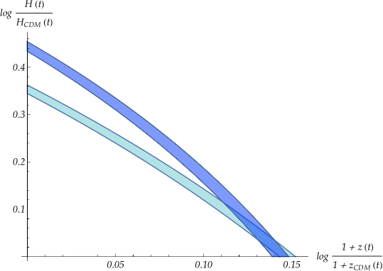
Figure 2: We plot $\log\frac{H(t)}{H_{\rm CDM}(t)}$ for $H(t)=H_{B}(t)$ and $H_{\Lambda^{\rm CMB}}(t)$ against $\log\frac{1+z(t)}{1+z_{\rm CDM}(t)}$, where $z(t)=z_{B}(t)$ and $z_{\Lambda^{\rm CMB}}(t)$, respectively. The color code is the same as in Fig. 1. By construction we have $\log\frac{H(t)}{H_{\rm CDM}(t)}\approx 0$ at $t_{\rm LS}$.

The CMB values $H_{0}^{\rm CMB}$ and $t_{0}^{\rm CMB}$ referred to in (11) are obtained from an analysis of the complete CMB data set [3]. This cannot be compared to our simple calculation where the only data we used from the CMB is the temperature $T(t_{0})$ measured today. To “compare” the $\Lambda$CDM model with our modified Friedmann equation one can choose to determine the two free parameters in the $\Lambda$CDM model, $\Lambda$ and $t_{0}$, using $z_{\Lambda}(t_{\rm LS})=1090$ and $H_{\Lambda}(t_{0})=H_{0}^{\rm SC}$, in the same way as we determined $t_{0}^{\rm B}$ and $B$. Denoting the time $t_{0}$ determined this way ${t}_{0}^{\rm SC}$, we find

$${t}_{0}^{\rm SC}=13.3\times 10^{9}\,{\rm y}.$$ (17)

${t}_{0}^{\rm SC}$ is quite a lot shorter than $t_{0}^{\rm CMB}$. In fact one would say that ${t}_{0}^{\rm SC}$ is uncomfortably short compared to the estimated oldest age of stars. The difference in $H(z)$ between our model based on the the modified Friedmann equation and the $\Lambda$CDM model, both with parameters determined by fitting to $z(t_{\rm LS})=1090$ and $H(t_{0})=H_{0}^{\rm SC}$, is shown for small values of $z$ in Fig. 3 (blue and orange regions, respectively). For comparison we have also shown $H(z)$ as determined from the best fit to the CMB data (green region). All curves approximately agree for large $z$, as is also seem on the figure. We have also included other independent measurements of $H(z)$.

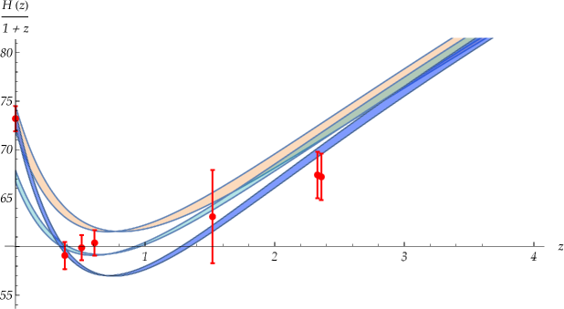
Figure 3: The blue area shows $H(z)/(1+z)$ for the modified Friedmann equation, while the green area shows $H(z)/(1+z)$ based on $\Lambda$CDM model with $H_{0}^{\rm CMB}$ and $\Lambda^{\rm CMB}$ taken from [3]. The orange area shows $H(z)/(1+z)$ based on $\Lambda$CDM model with $H_{0}^{\rm SC}$ and $\Lambda^{\rm SC}$ as described in the main text. Inserted in red are (apart from the SC data at $z\approx 0$) also independent data from other observations: first three points from the baryon acoustic oscillation data [6], the next from quasars [7] and the last two data points from Ly–$\alpha$ measuments [8, 9].

The error bars of the independent measured $H(z)$ are quite large, and the data points few, but if we make the simplest $\chi^{2}$ fit to test how well the theoretical curves agree with the data we obtain

$$\chi^{2}_{\rm red}({\rm B})=1.8,\quad\chi^{2}_{\rm red}(\Lambda^{\rm SC})=3.7,\quad\chi^{2}_{\rm red}(\Lambda^{\rm CMB})=4.0,$$ (18)

where the three reduced $\chi^{2}$ values refer to the blue, the orange and the green curves in Fig. 3. The orange curve seems to be disfavored compared to the blue curve. The main contribution to $\chi^{2}_{\rm red}(\Lambda^{\rm CDM})$ comes from a single data point, namely the point at $z\!=\!0$, which is of course precisely the source of the $H_{0}$ tension .

4 Discussion

Let us note that with $B$ fixed as described above our model gives a prediction for some of the standard variables like $\Omega_{\rm m}(t_{0})$ and $w(t_{0})$. The modified Friedmann equation (2) can be rewritten as

$$\Omega_{\rm m}(t)+\Omega_{B}(t)=1,\quad\Omega_{\rm m}(t):=\frac{\kappa\rho(t)}{3}\left(\frac{a}{\dot{a}}\right)^{2},\quad\Omega_{B}(t)=(1\!-\!F(x))(1\!+\!3F(x)),$$ (19)

where $x=Ba^{3}/\dot{a}^{3}$, as in eq. (2). $\Omega_{B}(t)$ is replacing the usual term $\Omega_{\Lambda}(t)$ in the $\Lambda$DCM model and there is no $\Omega_{\rm K}$–term from a spatial curvature as already noted. We now define $w_{B}(t)$ as

$$w_{B}(t):=\frac{2q(t)-1}{3\Omega_{B}(t)},\qquad q(t):=-\left(\frac{a}{\dot{a}}\right)^{2}\frac{\ddot{a}}{a},$$ (20)

and we find, using the definition $H(t)=100\,h(t)$ km s^-1Mpc^-1,

$$\Omega_{\rm m}(t_{0}^{\rm B})=0.268\pm 0.009,\qquad q(t_{0}^{\rm B})=-0.82\pm 0.01,$$ (21)

$$t_{*}=(7.26\pm 0.09)\times 10^{9}\,{\rm y},\qquad w_{B}(t_{0}^{\rm B})=-1.205\pm 0.006.$$ (22)

The value of $\Omega_{\rm m}(t_{0}^{\rm B})$ coming from our model is somewhat lower than the value extracted from the CMB data ($\Omega_{\rm m}(t_{0}^{\rm CMB})=0.315\pm 0.007$). However, our value of $\Omega_{\rm m}(t_{0}^{\rm B})\big{(}h_{B}(t_{0}^{\rm B})\big{)}^{2}$ is (almost) identical to the corresponding CMB–value since $\Omega_{\rm m}(t)h^{2}(t)\propto\rho_{\rm m}(t)$, where $\rho_{\rm m}(t)$ denotes the matter energy density, and where we in the matter dominated era have $\rho_{\rm m}(t)\propto 1/a^{3}(t)$. Thus, to the extent that $\Omega_{\rm m}(t_{\rm LS})$ and $h(t_{\rm LS})$ are independent of cosmological constant parameters like $\Lambda$ and $B$, one obtains an almost model independent value of $\Omega_{\rm m}(t_{0})\big{(}h(t_{0})\big{)}^{2}$ as long as one assumes the same value of $z(t_{\rm LS})$ (i.e. of $a(t_{0})/a(t_{\rm LS})$).

Maybe the most important prediction is that $w_{B}(t_{0}^{\rm B})\approx-1.2$. This is actually in agreement with certain fits to data (see for instance [5], section II.3 for a recent review), but is difficult to explain from physical healthy theories based on small modifications of the $\Lambda$CDM model, and usually $w(t)<-1$ is associated with the presence of so-called ghost fields. However, such ghost fields are not needed in our model and $w_{B}(t)\to-1$ for $t\to\infty$. No Big Rip will occur for the universe despite $w_{B}(t)<-1$, and the universe will at late times expand exponentially as indicated in eq.  (3).

Our modified Friedmann equation seems to be able to produce values of $H(z)$ which are in good agreement with the observed values, by fitting only to $T(t_{0})$ and $H_{0}^{\rm SC}$. Of course, for the model to genuine do better than the $\Lambda$CDM model one should repeat what is actually done to test the $\Lambda$CDM model, namely use the set of data from the CMB to fit a range of cosmological parameters and as a side result come up with a prediction for $H_{B}(t_{0}^{\rm B})$, based only the CMB data. If this could be done and the values of $t_{0}^{\rm B}$ and $B$ still agree with the values determined here, and the analysis of the fluctuations works out as well as it does for the $\Lambda$CDM model, one could say that our model has resolved the present $H_{0}$ tension. This requires a detailed understanding of how to derive in our model the fluctuations of geometry around the assumed Friedmann geometry. Presently we only know how to do that in the case where spacetime is two-dimensional. The extension to four-dimensional spacetime is still work in progress. Finally, it is also our hope that we will actually be able to calculate the value of the constant $B$ which appears in our modified Friedmann equation from the underlying microscopic model based on a certain $W_{3}$ algebra.

References

-
[1]
J. Ambjorn and Y. Watabiki,
“A model for emergence of space and time,”
Phys. Lett. B 749 (2015) 149, [arXiv:1505.04353 [hep-th]].
“Creating 3, 4, 6 and 10-dimensional spacetime from W3 symmetry,”
Phys. Lett. B 770 (2017) 252, [arXiv:1703.04402 [hep-th]].
“CDT and the Big Bang,”
Acta Phys. Polon. Supp. 10 (2017) 299, [arXiv:1704.02905 [hep-th]].
“Models of the Universe based on Jordan algebras,”
Nucl. Phys. B 955 (2020), 115044, [arXiv:2003.13527 [hep-th]]. -
[2]
J. Ambjørn and Y. Watabiki,
“A modified Friedmann equation,”
Mod. Phys. Lett. A 32 (2017) no.40, 1750224 [arXiv:1709.06497 [gr-qc]]. -
[3]
N. Aghanim et al. (Planck),
“Planck 2018 results. VI. Cosmological parameters,”
Astron. Astrophys. 641, A6 (2020), arXiv:1807.06209 [astro-ph.CO]. -
[4]
Adam G. Riess, Stefano Casertano, Wenlong Yuan,
J. Bradley Bowers, Lucas Macri, Joel C. Zinn, and Dan Scolnic,
“Cosmic Distances Calibrated to 1% Precision with Gaia EDR3 Parallaxes and Hubble Space Telescope Photometry of 75 Milky Way Cepheids Confirm Tension with CDM,”
Astrophys. J. Lett. 908, L6(2021), arXiv:2012.08534 [astro-ph.CO]. -
[5]
L. Perivolaropoulos and F. Skara,
“Challenges for CDM: An update,”
arXiv:2105.05208 [astro-ph.CO]. -
[6]
Shadab Alam et al. (BOSS),
“The clustering of galaxies in the completed SDSS-III Baryon Oscillation Spec- troscopic Survey: cosmological analysis of the DR12 galaxy sample,”
Mon. Not. Roy. Astron. Soc. 470, 2617–2652 (2017), arXiv:1607.03155 [astro-ph.CO]. -
[7]
Pauline Zarrouk et al.,
“The clustering of the SDSS-IV extended Baryon Oscillation Spectroscopic Survey DR14 quasar sample: measurement of the growth rate of structure from the anisotropic correlation function between redshift 0.8 and 2.2,”
Mon. Not. Roy. Astron. Soc. 477, 1639–1663 (2018), arXiv:1801.03062 [astro- ph.CO]. - [8] J. E. Bautista, N. G. Busca, J. Guy, J. Rich, M. Blomqvist, H. d. Bourboux, M. M. Pieri, A. Font-Ribera, S. Bailey and T. Delubac, et al. “Measurement of baryon acoustic oscillation correlations at with SDSS DR12 Ly-Forests,” Astron. Astrophys. 603 (2017), A12, arXiv:1702.00176 [astro-ph.CO].
- [9] A. Font-Ribera et al. [BOSS], “Quasar-Lyman Forest Cross-Correlation from BOSS DR11 : Baryon Acoustic Oscillations,” JCAP 05 (2014), 027, arXiv:1311.1767 [astro-ph.CO].
- [10] M. G. Dainotti, B. De Simone, T. Schiavone, G. Montani, E. Rinaldi and G. Lambiase, “On the Hubble constant tension in the SNe Ia Pantheon sample,” Astrophys. J. 912 (2021) no.2, 150, [arXiv:2103.02117 [astro-ph.CO]].