Phantom: A High-Performance Computational Core for Sparse Convolutional Neural Networks

Abstract.

Sparse convolutional neural networks (CNNs) have gained significant traction over the past few years as sparse CNNs can drastically decrease the model size and computations, if exploited befittingly, as compared to their dense counterparts. Sparse CNNs often introduce variations in the layer shapes and sizes, which can prevent dense accelerators from performing well on sparse CNN models. Recently proposed sparse accelerators like SCNN, Eyeriss v2, and SparTen, actively exploit the two-sided or full sparsity, that is, sparsity in both weights and activations, for performance gains. These accelerators, however, either have inefficient micro-architecture (Eyeriss v2, SCNN), which limits their performance, have no support for non-unit stride convolutions (SCNN) and fully-connected (FC) layers (SCNN, SparTen), or suffer massively from systematic load imbalance (SCNN, Eyeriss v2). To circumvent these issues and support both sparse and dense models, we propose Phantom, a multi-threaded, dynamic, and flexible neural computational core. Phantom uses sparse binary mask representation to actively lookahead into sparse computations, and dynamically schedule its computational threads to maximize the thread utilization and throughput. We also generate a two-dimensional (2D) mesh architecture of Phantom neural computational cores, which we refer to as Phantom-2D accelerator, and propose a novel dataflow that supports all layers of a CNN, including unit and non-unit stride convolutions, and FC layers. In addition, Phantom-2D uses a two-level load balancing strategy to minimize the computational idling, thereby, further improving the hardware utilization. To show support for different types of layers, we evaluate the performance of the Phantom architecture on VGG16 and MobileNet. Our simulations show that the Phantom-2D accelerator attains a performance gain of $12\times$, $4.1\times$, $1.98\times$, and $2.36\times$, over dense architectures, SCNN, SparTen, and Eyeriss v2, respectively.

1. Introduction

Neural nets have been around since the 1940s, however, the first practically applicable neural network, referred to as the LeNet (Le Cun et al., 1989), was proposed in 1989. This neural network was designed to solve the problem of digit recognition in hand-written numeric digits. It paved the way for the development of neural networks responsible for various applications related to digit recognition like an ATM. The slow growth and a little to no adoption of neural networks in the early days is mainly due to the massive computational requirements involved with their processing which limited their study to theoretical concepts. Over the past decade, there has been an exponential growth in the research on deep neural networks (DNNs) with many new high accuracy DNNs being deployed for various applications. This has only been possible because of two factors. The first factor is the advancements in the processing power of semiconductor devices and technological breakthroughs in computer architecture. Nowadays, computers have significantly higher computing capability. This enables the processing of a neural network within a reasonable time frame, something that was not achievable in the early days. The second factor is the availability of a large amount of training datasets. As neural networks learn over time, providing huge amounts of training data enables better accuracy. For example, Facebook receives close to a billion user images per day, whereas, YouTube has 300h of video uploaded every minute (Sze et al., 2017). This enables the service providers to train their neural networks for targeted ad campaigns bringing in billions of dollars of ad revenue. Apart from their use in social media platforms, DNNs are impacting many other domains and expect to make a huge impact. One of the domains where DNNs have contributed significantly is speech processing. Nowadays, many applications have been developed that use DNNs to perform real-time speech recognition with unprecedented levels of accuracy (Hinton et al., 2012; Collobert et al., 2011; van den Oord et al., 2016). Many technology companies are also using DNNs to perform language translation used in a wide variety of applications. Google, for example, uses Google’s Neural Machine Translation system (GNMT) (Wu et al., 2016) which uses recurrent neural networks (RNNs), a type of DNN, for their language translation applications. Autonomous driving has been one of the biggest technological breakthroughs in the auto industry since the invention of the internal combustion engine. It is not a coincidence that the self-driving boom came at the same time when high accuracy DNNs became increasingly popular. Companies like Tesla and Waymo are using various types of self-driving technology including visual feeds and Lidar for their self-driving solutions. One thing which is common in all these solutions is the use of DNNs for visual perception of the road conditions which is the main back-end technology used in advanced driver assistance systems (ADAS). Another crucial area where DNNs have become increasingly useful is medicine. Nowadays, doctors can use AI-assisted medical imagery to perform various surgeries. AI systems use DNNs in genomics to gather insights about genetic disorders like autism (Bi et al., 2018; Guo et al., 2017). DNNs are also useful in the detection of various types of cancers like skin and brain cancer (Baştürk et al., 2017; Siar and Teshnehlab, 2019). The advent of AI has also challenged many traditional security approaches that were previously deemed sufficient. The rollout of 5G technology has caused a massive surge of IoT-based deployments which traditional security approaches are not able to keep up with. Physical unclonability approaches (Qureshi and Munir, 2020b, 2019, 2021a) were introduced to protect this massive deployment of IoTs against security attacks with minimum cost overheads. These approaches, however, were also unsuccessful in preventing AI-assisted attacks using DNNs (Santikellur et al., 2019; Mursi et al., 2020). Researchers have now been forced to upgrade the security threat models to incorporate AI-based attacks (Mirsky et al., 2021; Miao et al., 2021). Because of a massive increase in AI-assisted cyber-attacks on cloud and datacenters, corporations and governments have realized that the best way of defeating offensive AI attacks is by incorporating AI-based defensive strategies.

Overall, the use of DNNs in various applications has seen exponential growth over the past decade and this trend has been on the rise for the past many years. The massive increase in DNN deployments on the edge devices requires the development of efficient processing architectures to keep up with the computational requirements for successful DNN inference.

Convolutional neural networks (CNNs) for vision artificial intelligence (AI) applications have reached an unprecedented accuracy ever since the introduction of AlexNet (Krizhevsky et al., 2012) about a decade ago. Many of the previously proposed high accuracy CNNs (Krizhevsky et al., 2012; Simonyan and Zisserman, 2014; He et al., 2015; Szegedy et al., 2015) have tremendous amounts of computations owing to a large number of model parameters. These parameters and the associated massive number of computations generate exorbitant amounts of data in the form of partial sums (psums) and feature maps. This massive data, in addition to the model parameters, raise concerns in regards to both compute and memory bandwidth. In addition, it also raises concerns about energy consumption of a neural network accelerator (NNA), since, on-chip memory is not sufficient to store the entire model, which, in some cases, can be in the order of hundreds of MBs. To support this massive model size of a CNN, off-chip DRAM memories are generally employed. It has been shown that the energy cost per fetch for 32b coefficients in an off-chip LPDDR2 DRAM is about 640pJ, which is about $6400\times$ the energy cost of a 32b integer ADD operation(Horowitz, 2014). The power dissipation resulting from just the DRAM accesses would be well beyond the limits of an embedded mobile device employing the NNA.

Modern CNNs owe their high accuracy to deep layers and the non-linearity in their design. Typically, non-linearity is added by incorporating activation functions, the most common being the rectified linear unit (ReLU) (Sze et al., 2017). The ReLU converts all negative values in a feature map to zeros. Since the output of one layer is the input to the next layer, many of the computations, within a layer, involve multiplication with zeros. These feature maps containing zeros are referred to as one-sided sparse feature maps. The multiplications resulting from this one-sided sparsity wastes compute cycles and decreases the effective throughput and hardware utilization, thus, reducing the overall performance of the accelerator. It also results in high energy cost as the transfer of zeros to/from off-chip memory is a wasted memory access. In order to reduce the computational and memory access volume, previous works (Albericio et al., 2016; Zhang et al., 2016; Chen et al., 2017) have exploited this one-sided sparsity and displayed some performance improvements.

Compression of DNN models was introduced the first time in (Han et al., 2016). Han et al. (Han et al., 2016) iteratively pruned the connections based on parameter threshold, and performed retraining to retain accuracy. This process resulted in two-sided sparsity, i.e., sparsity in both weights and activations, which led to approximately 9$\times$ model reduction for AlexNet, and 13$\times$ reduction for VGG-16. It also resulted in 4 - 9$\times$ effective compute reduction (depending on the model). These gains, in theory, are very promising, however, designing an accelerator that leverages the two-sided sparsity is quite challenging because of the following reasons:

1) Inconsistency in Data Accesses: Sparsity is generally exploited through gating of computation whenever a zero is read in either weight or activation data. This type of gating translates into energy savings but has no impact on throughput as the compute cycle is wasted and no effective work is performed during a zero read. Complex read logic needs to be implemented to discard the zeros, and instead perform effective computations on non-zero data. Some previous approaches (Chen et al., 2019; Han et al., 2016) use compressed sparse column (CSC) format to represent sparse data. These formats have variable lengths and make “looking ahead” difficult if both the weight and the activation sparsity is being considered. Other than that, developing the complex control and read logic to process these formats can be quite challenging.

2) Load Imbalance and Under Utilization of the Processing Element (PE) Array: Many accelerator architectures have a two-dimensional array of PEs that process the data in a consistent manner to maximize the hardware utilization. Different dataflows have been developed that efficiently schedule the data onto the PEs to maximize the throughput(Sze et al., 2017). Sparsity brings inconsistency in the scheduling of data, introducing workload imbalance. The subsection of PEs which are provided with more sparse data have idle times while those provided with dense data are fully active. This bounds the throughput of the accelerator to the most active PEs, and therefore, leads to the under utilization of the PE array.

Considering the aforementioned issues, many previously proposed accelerators attempt to strike a balance between hardware complexity and performance improvements. Eyeriss v2 (Chen et al., 2019) attempts to address the two-sided sparsity by using CSC format for both the activations and weights. It, however, fails to address the systematic load imbalance introduced due to variations in the density of the sparse matrices. It also requires complex read logic embedded within a PE that drastically increases the area by $\sim$ 93% when compared to the original Eyeriss (Chen et al., 2017). EIE (Han et al., 2016) exploits the two-sided sparsity, albeit only in fully-connected layers. EIE’s performance is equivalent to one-sided sparsity as it discards zeros in the filter but wastes compute cycles due to being idle. Sparse CNN (SCNN) (Parashar et al., 2017) targets two-sided sparsity but suffers heavily from inefficient microarchitecture and systematic load imbalance as explained in (Gondimalla et al., 2019). It, also, can not handle non-unit stride convolutions and FC layers. SparTen (Gondimalla et al., 2019) addresses the issues in previous architectures and attempts to strike a balance between data reuse and load imbalance. Instead of CSC format, SparTen, instead, uses sparse bit mask to represent the location of zeros and non-zero data values. SparTen, however, needs an offline load balancing strategy, which it refers to as Greedy Balancing, to address the systematic load imbalance. This form of balancing adds extra latency and complicates the synchronization of various compute threads. In addition, SparTen, like SCNN, has no support for FC layers.

To address all the issues described above, we propose Phantom, a flexible and high throughput neural computational core which promises high hardware utilization. The core works for both dense and sparse networks by dynamically mapping valid computations on the processing threads. The core also addresses the systematic load imbalance by using a two-level, dynamic, load balancing strategy. Unlike some of the previous works, the core can work on any input layer, be it CONV or FC, and supports any type of convolution (regular or separable). In summary, the main contributions of this work include:

• A multi-threaded neural computational core architecture, called Phantom, designed to maximize the hardware utilization and throughput of CNN models. Phantom exploits the sparsity in both weights, and activations, simultaneously, by incorporating simple, yet powerful circuits like “Lookahead Mask”, “Top-Down Selector” and “Thread Mapper”. These circuits, when used in conjunction, map the effective, non-zero computations onto an array of multiplier threads within a PE. The core also has the capability to skip huge number of non-essential computations (zero_w $\times$ zero_a, zero_w $\times$ non-zero_a, non-zero_w $\times$ zero_a), while simultaneously favoring essential computations (non-zero_w $\times$ non-zero_a), without wasting compute cycles (subscripts “w” and “a” here refer to weights and activations, respectively). This drastically improves the core’s hardware utilization, consequently improving the throughput.

• Addressing the systematic load imbalance by using a two-tiered, on-the-fly, load balancing strategy. Unlike some previous approaches, this balancing does not require offline processing or modification of the CNN model.

• Generating a two-dimensional (2D) mesh architecture of Phantom neural computational cores, which we refer to as Phantom-2D accelerator. Unlike some previous works that only support either CONV layers or FC layers, we show how Phantom-2D supports different CONV types (unit and non-unit stride) and FC layers, in addition to supporting both sparse and dense CNN models. Simulations show that the Phantom-2D accelerator has a performance gain of $12\times$, $4.1\times$, $1.98\times$, and $2.36\times$, over dense architectures, SCNN, SparTen, and Eyeriss v2, respectively, while retaining the energy efficiency of SparTen.

2. Related Work

Many dense architectures have been proposed in the literature that optimize compute (Gokhale et al., 2017; Jouppi et al., 2017; Lin et al., 2016) and memory bandwidth (Du et al., 2015; Liu et al., 2015) for CNN inferences. Quantization of weights and activations using log (Miyashita et al., 2016; Vogel et al., 2018) and linear (Lin et al., 2016; Gupta et al., 2015) techniques further reduce the memory footprint. This does not result in a significant loss in accuracy and reduces the CNN model size by a considerable amount. Hardware implementations like Envision(Moons et al., 2017), VWA(Chang and Chang, 2020), NeuroMAX(Qureshi and Munir, 2020a), UNPU(Lee et al., 2018), and Stripes(Judd et al., 2016), show how reduced bit precision, efficient dataflow, and quantization, translates into increased throughput and savings in energy. Efficient data reuse-based accelerators (Alwani et al., 2016; Chen et al., 2017) maximize the data reuse within different layers to minimize the memory accesses, thereby, reducing energy consumption. Separable accelerators (Liu et al., 2019; Bai et al., 2018) implement efficient hardware on FPGA for accelerating separable convolutions. These accelerators, however, cannot handle a vast majority of CNNs that employ regular convolutions and FC layers. Bit-serial accelerators (Sharify et al., 2019; Delmas et al., 2018) use booth encoding to suppress the use of zero bits, and, thereby, reduce the total computations. These schemes, however, transfer zeros to and from memory which incurs SRAM area and energy. CirCNN(Ding et al., 2017) uses block circulant matrices for weights to improve the performance. It, however, utilizes complex hardware to perform the FFT operations, and also, does not capture full sparsity. In-memory accelerators (Ankit et al., 2019; Shafiee et al., 2016) use simple analog logic to implement matrix multiplications within memory. These accelerators, however, cannot exploit sparsity as it requires complex ALU and buffering logic. Analog circuits also suffer heavily from noise and process variations which can drastically reduce the CNN accuracy.

Sparse architectures try to reduce the compute and data volume by exploiting the naturally occurring zeros in weights or activations (one-sided), or both weights and activations (two-sided). Cnvlutin(Albericio et al., 2016) and Cambricon-X(Zhang et al., 2016) exploit one-sided sparsity of either weights or input maps but not both. Cnvlutin, also, does not avoid transfer of zeros and only skips cycles for activations. Cambricon-X does not store activations in compressed format while Cambricon-S(Zhou et al., 2018) forces regularity by employing coarse grain pruning that affects accuracy. Even though it discards zeros during computation, it still retrieves and stores them. Tensaurus (Srivastava et al., 2020b) accelerates dense and sparse tensor factorizations by introducing a new dataflow which they refer to as compressed interleaved sparse slice (CISS) dataflow. Tensaurus, however, is capable of supporting only one-sided sparsity. Some recent sparse GEMM (SpGEMM) accelerators (Srivastava et al., 2020a; Hegde et al., 2019; Qin et al., 2020; Zhang et al., 2020; Pal et al., 2018; Qureshi and Munir, 2021b) target general sparse-matrix, sparse-matrix multiplications. Extensor (Hegde et al., 2019) and Sigma (Qin et al., 2020) use output stationary (inner product) dataflow for sparse matrix multiplications. Inner product, however, is inefficient against highly sparse matrices because every element of the rows and columns must be traversed even though there are less effectual computations (non-zero $\times$ non-zero). This leads to a massive amount of wasted computations. SpArch (Zhang et al., 2020) and OuterSPACE (Pal et al., 2018) use input stationary (or outer-product) dataflow to avoid the inefficiencies associated with the inner-product dataflow. Outer-product, however, gives poor output reuse as the partial outputs generated are more in quantity than the final outputs which can cause significant memory traffic. Finally, MatRaptor (Srivastava et al., 2020a) introduces channel cyclic sparse row (C²SR) dataflow for better reuse and memory efficiency. It is a modified version of the CSR format but requires complex encoding for output matrices. Finally, SCNN, SparTen, and Eyeriss v2, exploit the full two-sided sparsity, but, as explained previously, suffer from either inefficient micro-architecture, no support for FC layers and non-unit stride convolutions, complex PE design to incorporate CSC compression format, or systematic load imbalance. Phantom addresses all of these issues while also providing higher performance and energy efficiency.

Figure 1. $3\times 3$ convolution example

Figure 2. Sparse mask representation

3. PHANTOM

This section describes the architecture and inner workings of the Phantom core. Recall from Section 1 that the Phantom core in itself provides two major contributions. First, it considers both activation and weight sparsity simultaneously and looks ahead into future computations to determine only the valid MAC operations (non-zero_w $\times$ non-zero_a). Second, because of the multi-threaded design of the PEs, the scheduling of data into each thread is handled dynamically in a non-linear fashion, based on the sparsity of input and weight matrices. This ensures that only valid computations are mapped on to the multi-threaded PEs and that the compute cycles are not wasted. This is opposed to the designs which schedule data into the PEs in a constant manner and gate the computations whenever zeros are read, thereby, wasting the compute cycles.

Figure 1 shows a $3\times 3$ convolution example, where a $3\times 8$ input is convolved with a $3\times 3$ filter to produce a $1\times 6$ output. The six individual convolution chunks which produce the output are also shown. The effective and ineffective multiplications are shown in blue and red, respectively. It can be seen that, on average, $55\%$ computations involve multiplication with zeros which results in wasted compute cycles. This causes a significant drop in the effective throughput, as many cycles are wasted in zero multiplications. The Phantom core addresses this issue and uses look-ahead masking to maximize the effective throughput by skipping ineffectual computations involving zeros.

3.1. Sparse Mask Representation

Unlike the recent approaches that use compressed sparse row (CSR) or CSC formats to represent non-zero data (Zhang et al., 2016; Albericio et al., 2016; Han et al., 2016), we use a binary mask called sparse mask for both weight and activation data. Sparse mask provides an efficient and simplistic way for data representation and enables identification of zero and non-zero data without explicitly storing zeros. It also does not require storage of count and data pointers which are needed for CSC (and CSR) formats. Figure 2 shows the equivalent sparse mask representation and storage of the input and the weight matrix shown in Figure 1. For a particular matrix, two arrays are stored in the column major format. The data array contains the non-zero data, whereas, the binary array contains the sparse mask. The ones in the sparse mask array represent the location of stored non-zero values, whereas, zeros represent unstored zero data. To process a specific type of convolution, the sparse mask and the data array is broken into chunks and scheduled to the core. Although, the core can work on any type of CONV or FC layers, for ease of understanding, we will explain the working of Phantom core using the $3\times 3$ unit stride convolution example, shown in Figure 1.

Figure 3. Phantom block diagram

Figure 4. ANDing of sparse masks

3.2. Core Architecture

Phantom core accepts data in the sparse mask format and consists of 5 main blocks, as shown in Figure 3. The lookahead mask (LAM) and the top-down selector (TDS) blocks use the sparse mask to extract the information about the valid computations and thread selection. The thread mapper (TM) uses the information from the previous blocks to efficiently map input and weight data onto the data registers of the multiplier threads within the compute engine (CE). The CE consists of an array of multi-threaded PEs and level 1 (L1) configurable adders. The output buffer (OB) block consists of an array of FIFO buffers and level 2 (L2) accumulators which generate the final output.

3.3. Lookahead Masking

Dot product between two vectors is the basic unit of computation in a convolution operation. Considering two-sided sparsity, there are 4 possible multiplication outcomes as a result of sparse vector-vector dot product.
A) zero_w $\times$ zero_a
B) zero_w $\times$ non-zero_a
C) non-zero_w $\times$ zero_a
D) non-zero_w $\times$ non-zero_a
The only valid multiplication is when a non-zero weight data is multiplied by a non-zero activation data. As the name implies, the lookahead mask (LAM) block looks ahead into n convolution chunks to determine the locations of valid multiplications. We refer to the value $n$ as the lookahead factor ($L_{f}$) . To perform its task, the LAM block performs an AND operation between the sparse masks of the weight matrix and the input chunks to generate output masks. Figure 4 shows the process of ANDing. Here, SPM_W and SPM_IA are the sparse masks of the weight and the input matrix of the example in Figure 1. Six output chunks are generated based on the AND operation.

To perform this ANDing, the LAM consists of a series of n AND gates, as shown in Figure 5(a). Bitwise ANDing is perfomed between the weight and the activation sparse mask. For this example, we set the value of $n$ to 3. This means that to generate six output masks in Figure 4, two cycles will be needed for the six AND operations.

Figure 5. Lookahead masking (a) Sequence of parallel AND gates (b) Output for test case

Figure 5(b) shows the output of LAM for the test example. The $n=3$ AND gates produce outputs (LAM₁, LAM₂, LAM₃) on every cycle edge. It takes 2 cycles to slide over the entire $3\times 8$ activation matrix. The ones in the outputs of AND gates represent the location of a valid vector-vector dot product whereas the zeros represent a product resulting in a zero. Overall, it can be seen that by using a sequence of n-AND gates, we can accurately determine the positions of valid computations in $n$ convolution chunks.

3.4. Top-Down Selector

The top-down selector (TDS) receives the LAM outputs on every cycle edge and selects a sub-sequence of LAM outputs that can maximize the utilization of multiplier threads in the PEs within the CE. There are a total of p parallel selectors, with p equal to the total number of PEs in the CE. In this design, we consider $p=3$, since there are a total of 3 PEs in the CE. We develop two selection algorithms for the TDS block namely, in-order selection and out-of-order selection.

3.4.1. In-Order Selection

Figure 6(a) shows the process of in-order selection. The three selectors work on the three comma-separated columns in parallel. The selection is performed iteratively in an ordered fashion on the entire column in a top-down manner. For column 1 in Figure 6(a), the first selector loops through the first $n$ elements in the current iteration, i.e., $011$(black), $011$(blue), and $010$(orange). Here, $n$ equals the lookahead factor ($L_{f}$), which is 3 in this design. The first $011$ (in black) is assigned the highest priority and is selected. The selector counts the number of ones from this entry and stores the result. The selector then proceeds to the next entry, i.e., $011$ (in blue), and counts the number of ones. If the combined sum of the number of ones of the current and the previous entry is greater than $n$, the current and the next entries, in the current iteration are not considered, and instead, replaced by zeros. Here, we see that 011(in black) + 011(in blue) = 4 ¿ ($n=3$). Therefore, only the first 011 (in black) is selected and the rest two entries are replaced by zeros in the first iteration. Here, every 1 in the selected output corresponds to a valid multiplication. Since, there are a total of 3 multiplier threads within a single PE, if the selected values contain a total of three 1s, then all the threads within a PE are utilized, giving a utilization of 100% (as shown in Figure 6(a)). The utilization decreases if the order in which the entries appear do not align with the priority of selection. The circles around the values and the numbers on top represent the iteration number during which the particular value was selected by the selector. In the second iteration, the selector goes on to the first unselected value (011 in blue) and follows the same selection process. It takes a total of four iterations (cycles) for the selector to select all the values in the first column, as shown in Figure 6(a). We can also see that the second and the third columns require a total of three cycles for selection, but need to wait one additional cycle for the selection of the first column to complete. This can cause computational idling and under-utilization of the PE multipliers.

Figure 6. Top down selector (a) In-order selection (b) Out-of-order selection

3.4.2. Out-of-Order Selection

In-order selection is highly dependent on the order in which the inputs appear. This can lead to under-utilization of the multiplier threads in the PE, as shown in Figure 6(a). Figure 6(b) shows the out-of-order selection method, where after the selection of the 1^st entry (011 in black), all next entries (011 in blue, 010 in orange) in an iteration are considered for selection. Therefore, as shown in Figure 6(b), in the first iteration, after the selection of 011(in black), the next value 011 (in blue) is not considered (011 + 011 = 4 ¿ $n$) but the subsequent value 010 (in orange) is considered because 011(in black) + 010 (in orange) $\leq n$ . This small, yet efficient change greatly improves the thread utilization and consequently the throughput, as shown in Figure 6(b). Figure 7 shows the implementation of the out-of-order selection variant of the TDS for the first column in Figure 6(b). A small block memory, having independent read and write ports, receives the LAM outputs on every cycle. P1 and P2 are the high and low priorities, respectively. The read address (rd_addr) of the memory increments every time a value is selected and the tag bits are set to 1 for those values. The tag bits serve the purpose of accumulation during the output buffering (explained in Section 3.7). The priority of selection is reversed on the next input to ensure that the values missed in the previous iteration are given the highest priority in the current iteration. map₁₁, map₁₂, and map₁₃ are the final outputs, as shown in Figure 8. The hardware overhead of the out-of-order selector is roughly 1.03$\times$ that of the in-order selector variant, but can increase the hardware utilization by as much as 60%. Phantom, therefore, employs the out-of-order selection variant of the TDS for higher thread utilization and efficient mapping.

Figure 7. Out-of-order selection implementation

Figure 8. TDS out-of-order variant input-output

Figure 9. Thread mapping

3.5. Thread Mapper

The Thread Mapper (TM) takes the input from the TDS (map_1x, map_2x, and map_3x) and uses this information to map the length equalized sparse data (weight and activation) onto the internal registers of the multi-threaded PEs. The length equalization is done by adding appropriate zeros at specific locations using the sparse masks. Figure 9 shows the map operation for the three PEs in this design. Out of the 2⁹ = 512 combinations, the mapper only needs to store those for which the total number of ones do not exceed the multiplier count of each PE (3 in this case). This drastically reduces the total combinations needed to be stored (${9\choose 0}+{9\choose 1}+{9\choose 2}+{9\choose 3}$ = 130, a 74% reduction in the memory footprint). Each PE has a 50 bit internal register, out of which, 48 bits are the data bits, and 2 bits are the L1 adder control bits. The first 48 bits are divided into a set of 16 bits (8 bits for both activations and weights). The total memory requirement for storage of all three mappers is approximately 2.5 kB. One key observation from Figure 9 is that the mapper 2 and 3, map the data in a similar fashion as the mapper 1, but only use different location bits for weights and data. We, therefore, remove the two mappers (map_2x and map_3x), and only use one mapper (map_1x) sequentially 3 times, and adjusting the location bits afterwards. This only incurs an initial latency of 2 cycles but reduces the memory footprint by approximately 66% (2.5 kB to 0.83 kB). Appropriate delay registers are added in the PEs to account for the initial delay.

Figure 10. Compute engine (a) Multi-threaded design (b) Scheduling for example in Figure 1

3.6. Compute Engine

The Phantom core uses a multi-threaded CE block. In this particular design, the CE block consists of 3 multi-threaded PEs, with each PE containing 3 multiplier threads, as shown in Figure 10(a). The mapper maps the data to the individual threads which perform independent computations. The outputs of the threads, local to a particular PE, are provided to the L1 adder. The L1 adder is provided the configuration bits from the last 2 bits of the mapper (Figure 9). There are 4 cases for the configuration bits:
C1: 00 -¿ The individual outputs of the multiplier threads within the PE are not added and simply passed.
C2: 01 -¿ The outputs of the first two multiplier threads (th_0,x,th_1,x) are added, whereas, the third one (th_2,x) is passed as is.
C3: 10 -¿ the outputs of th_1,x and th_2,x are added and the output of th_0,x is passed as is.
C4: 11 -¿ the outputs of all the multiplier threads are added.
Figure 10(b) shows the cycle by cycle scheduling of the multiplier threads with data (weights and activations) mapped using the logic in Figure 9. The mapping inputs (map₁₁, etc.) and L1 adder configuration outputs are also shown. It can be seen that all the multiplier threads are efficiently utilized even though the output is 55% sparse (counting number of zeros from the left side of Figure 8, 30/54). The hardware utilization during the 1^st and 2^nd cycle is 100%, whereas, for the 3^rd cycle, it is 66%. The reason for low utilization in the last cycle is because the input is at the boundary and the LAM block does not have more data to look ahead into.

Figure 11. Output buffer for example in Figure 1

Figure 12. L2 accumulation for the example in Figure 1

3.7. Output Buffer

The final block in the Phantom core is the output buffer (OB). OB is responsible for buffering the outputs of the CE, and accumulation of data using the L2 adder to generate the final outputs. The buffering is performed using a system of $m$ first-in, first out (FIFO) buffers, where $m$ is equal to the total number of multiplier threads in the CE (9). Figure 11 shows the OB block for the example in Figure 1. F1-F9 are the 9 fifos receiving data from the L1 adders in the CE. The ones (in blue) and zeros (in red) within the parenthesis represent the tag bits which were set by the TDS block, as shown in Figure 7. Accumulation is performed in two stages by the same colored fifos (F1 + F4 + F7), (F2 + F5 + F8), and (F3 + F6 + F9). The outputs are either valid or partial, based on the associated tags. If the tags of all the values being accumulated are equal to 1, the output is considered valid, otherwise, it is considered partial. For the example in Figure 1, the outputs in L2 adder are calculated as shown in Figure 12. The two stages of accumulation are also shown. In the first stage, the previously accumulated partial output is added to the new entry in the fifo to make the output valid. This is done by checking the tag bits in the partial output and adding the missing tag 1 in the new value to generate the valid output from partial output. In the second stage, new partial values are generated by replacing the used tag 1 value in the first stage by 0 and accumulating the rest of the tag 1 values. The process ends once the input is exhausted and all the tag 1 values have been accumulated to generate valid outputs.

Figure 13. Output sparse mask generation

3.8. Output Encoding

Figure 13 shows the process of output sparse mask generation. Unlike the weights, the output activation sparsity is dynamic and the sparse mask needs to be generated on-the-fly. From Figure 4, we can see that the presence of even a single one in the LAM outputs represent a non-zero output. To determine the output sparse mask, the same metadata can be used. The first step involves reduction of the individual LAM outputs to a single bit (LAM_xr), based on an all-zero check, as shown in Figure 13(a). This generates the sparse mask for the outputs before ReLU. Note that the LAM values are taken from the test example (Figure 1). Figure 13(b) shows the second step after ReLU, where the negative outputs, and their corresponding sparse mask locations, are converted into zeros. This final sparse mask is stored as is, whereas, the output is shifted first to omit zero data entries, and then stored.

This concludes the processing in a single Phantom core. In the next section, we will introduce Phantom-2D; a two-dimensional accelerator having a system of Phantom cores for processing CNN layers during the inference process.

Figure 14. Phantom-2D architecture

4. Phantom-2D

The previous sections describe the working of the various blocks in the Phantom core. The individual core works by computing a dot product between a weight matrix and a subsection of the input feature map to compute a subsection of the output feature map. To compute the full output feature map, corresponding to a particular layer, we design a two-dimensional accelerator comprising of the Phantom cores, which we refer to as Phantom-2D, as shown in Figure 14. We envision that the Phantom-2D accelerator connects to a memory bus and accepts data and instructions from a CPU. The accelerator contains on-chip SRAMs (weight, input, and output), the inter-Core balancer and scheduler, the $R\times C$ compute matrix, comprising of Phantom cores, and the accumulator circuits.

4.1. R$\times$C Compute Matrix

The compute unit consists of an $R\times C$ matrix of the Phantom cores and $R$ adders for channel accumulation. The design choice for $R$ and $C$, and the dataflow associated with the transfer of data across various Phantom cores, is based on the following design goals:

• To maximize the data reuse (weights and input) across multiple input subsections.

• To optimize the data scheduling across various Phantom cores to maximize the theoretical hardware utilization.

• To support all layers of a CNN. This includes support for a variety of CONV layers and the FC layers.

Looking deeper into the dimensions and configurations of various popular CNN models (VGGnet (Simonyan and Zisserman, 2014), Resnet(He et al., 2015), MobileNets(Howard et al., 2017; Sandler et al., 2018), Googlenet(Szegedy et al., 2015) etc), we observe that the channel count for various CNN layers is almost always a multiple of 4. In the Phantom-2D architecture, the channels in a CNN layer are broken along the columns. Therefore, to ensure that the cores are engaged most of the time, and thus, satisfy G2, we set the $C$ value equal to $4$. Similar rationale applies for the choice of $R=7$. The input subsections are broken along the vertical axis and distributed along the rows. Most of the popular CNNs have an input layer size (width or height) $S$, a multiple of $7$, thus, having $R=7$, ensures equal distribution of chunks of data among all the cores.

4.2. Load Balancing

The design choice for $R\times C$ matrix is highly dependent on the layer dimensions of various CNNs. It, however, has no relevance to the static and dynamic sparsity in weights and inputs, respectively. Efficient reuse of data is one of the key requirements to minimize the memory accesses, repeatedly, for the same data. This reuse, however, amplifies the computational imbalance among different PEs. If the same filter is held in the local memory of the PEs and the input subsections are swept across the PEs, the subsections with higher density would inevitably take more cycles to compute the output, compared to the PEs receiving the subsections with lower density. This varying sparsity of the input maps would create a system-level load imbalance among the PEs which would be exposed during the next filter broadcast. Holding the input maps and sweeping the filters would also have similar results, as would the buffering of data. In order to address this system-level load imbalance, we incorporate a two-level load balancing strategy in the Phantom architecture. The Inter-Core balancer (Figure 14), balances the computational load dynamically using the density of the weight matrix such that each phantom core works on the weight matrices with the same/similar density over the CNN layers (as described in Section 4.3.1 with an example). This balancing is only performed when the weight data is actively being reused (e.g. in regular and depthwise seperable CONV). The second balancer, referred to as Intra-Core balancer, is local to each core, and performs column-wise balancing of the weight matrix. This balancer is always enabled, regardless of the layer, and significantly improves the individual multiplier thread scheduling performed by the TDS.

In the subsequent sections, we demonstrate, with examples, the designed dataflow for various CONV and FC layers. We choose the input sizes that fit well with the layer sizes of actual CNNs. We also show how the balancing is performed to prevent idling of the cores, which in turn, maximizes the throughput, all the while ensuring high data reuse.

Figure 15. Regular/depthwise convolution

4.3. Regular/Depthwise Convolution

Figure 15 shows a $3\times 3$ depthwise separable convolution example, where 4, $3\times 3$ filters are convolved with a $9\times 5\times 4$ input to generate a $7\times 3\times 4$ output. We choose these size parameters as an example because they fit well when considering the layer sizes of the actual CNNs. The Figure also shows the scheduling and mapping of data on to the $R\times C$ matrix. The input is broken down into $n$ chunks along the rows, where, $n$ is the number of rows of the output. These $n$ chunks are then scheduled along the rows of the $R\times C$ matrix. Each Phantom core processes a $3\times 5$ input chunk to generate a $1\times 3$ output chunk. The filters F0 to F3 represent the channel wise filters, with each column of the $R\times C$ matrix processing a different channel. The reuse of filters (G1) along the rows is also shown. The non-unit stride convolutions follow the same dataflow. Because of the efficient dataflow, and choice of the $R\times C$ dimensions, all Phantom cores are provided data for a particular processing chunk, thereby, achieving a 100% inter-core utilization (G2).

4.3.1. Inter-Core Balancing

The inter-core balancing is performed for the layers that support filter reuse because of the static nature of the weights. In the proposed dataflow, the layers that support filter reuse are the regular and the depthwise separable convolution layers. As shown in Figure 15, each $R\times C$ matrix column, at any given time, processes the same filter. The filters are scheduled in a low latency, more dense and high latency, less dense approach. Assuming that during the first iteration, the four filters (F0, F1, F2, F3) are broadcasted and the first column’s processing latency is the lowest. In the next filter broadcast, the next set of filters will be broadcasted in such a way that the filter with the highest density and the associated input channel will be scheduled to the first column. In a similar fashion, as the columns proceed to completion, the next filters are scheduled based on the order of their completion. This ensures that the processing completes uniformly across all the columns so that the idle time for the individual phantom cores is minimized. Computation of density is trivial as it involves finding the total number of ones in the sparse mask of the filters, and thus, requires minimal resources.

Figure 16. Pointwise convolution

4.4. Pointwise Convolution

Figure 16 shows a pointwise convolution example where a set of $1\times 1\times 36\times 7$ sparse filters convolve with a $3\times 3\times 36$ sparse input to produce a $3\times 3\times 7$ output. These dimensional parameters are a good representative of the layer dimensions of actual CNNs. Figure 16 also shows the dataflow and the mapping of the various computations involved for this example. It can be seen that the $7$ filters are scheduled along the $7$ rows of the Phantom cores with each row processing equal number of channels along the columns. The channels are equally divided based on the number of combined multiplier threads in each Phantom core. Since, in this design, each Phantom core consists of 3 PEs, with each PE containing 3 multipliers (Figure 10), the channels are divided equally into batches of 9 and scheduled along the columns to maximize the hardware utilization (G2). To enhance data reuse (G1), each weight matrix is held locally in a particular core while the input is swept across it. The input is scheduled in a channel-first manner, followed by rows, and then columns. Figure 16 only shows the generation of the first column of the output. After all the rows for a particular channel have been exhausted, the next column is evaluated in a similar fashion till all the columns have been swept through. The L3 adder circuit gathers all the partial outputs from the cores along the columns to generate the required outputs.

Figure 17. FC layer processing

4.5. FC Layers

FC layers are an inherent part of modern CNN designs and, therefore, need to be accounted for in CNN accelerator designs (G3). AlexNet and VGG-16 both have FC layers with activation vectors that are 4K long and weight matrix that is 4K $\times$ 4K long. Similarly, Mobilenet has an FC layer with activation vector that is 1K long and weight matrix that is 1K $\times$ 1K long. The FC parameters comprise of a total of 24.3% of all the parameters in the Mobilenet. FC computations, therefore, are crucial and need to be accounted for in CNN accelerator designs (G3). Figure 17 shows an FC computation example where a length 36 sparse input vector (R₀-R₃₅) is element-wise convolved with a $36\times 49$ sparse weight matrix to generate a length $49$ output vector. Figure 17 also shows the dataflow and the computational mapping of the example onto the Phantom cores in the Phantom-2D architecture. Similar to the pointwise convolution, the input and the weight channels are broken into 4 batches of length 9 and scheduled across the columns. The input vector, is held stationary (input stationary) across the rows and the individual weight vectors are swept over the input vector to generate the partial outputs. Similar accumulation is performed by the L3 adders to generate the final outputs.

Figure 18. Intra-core balancing (a) Test example (b) Without balancing (c) With balancing

4.6. Intra-Core Balancing

The Intra-Core balancer performs thread-level balancing inside every Phantom core. This is opposed to the Inter-Core balancer which performs balancing across all the Phantom cores in the Phantom-2D architecture. Recall that the TDS (Section 3.4) operates in a column-wise manner where each column of the LAM outputs are evaluated concurrently, as shown in Figure 6. Also, recall that the total number of ones selected by the TDS per column are less than or equal to the number of multiplier threads per PE (3 in this case). Because of the column-wise selection, the TDS latency is bounded by the column with the highest density. Figure 18(a) shows a test example to explain the intra-core balancing and its significance. Figure 18(b) shows the core operation without any balancing. The first column of the weight matrix has the highest density. This is also reflected in the generated LAM values. This uneven distribution results in the first column taking the highest number of cycles, whereas, the second and the third column selection completing in only one cycle, as shown in Figure 18(b). This stalls the core as the core must wait for the first column to complete all 3 cycles before processing the next block which significantly decreases the thread utilization of the core (Valid Computations/(Cycles $\times$ PEs $\times$ ThreadsPerPE) = 9/(3 $\times$ 3 $\times$ 3) = 33%).

Figure 18(c) shows how the intra-core balancer mitigates this issue by efficient distribution of the load, prior to the TDS operation, in a relatively simplistic manner. A right circular shift is performed on LAM₂ and LAM₃ values, as shown in Figure 18(c). This modifies the load distribution among the three LAM columns. Operation of the TDS this time, ensures the selection of all three columns in one cycle. A circular left shift is performed on the generated map inputs (map₁₁ = 111 000 000, map₁₂ = 000 111 000, map₁₃ = 000 000 111) in the same manner as the circular right shift in the first step, to ensure a valid mapping by the mapper. The updated map values, after shifting, are shown in Figure 18(c). The updated map values are then used in the map_1x without adjustment in the location/index (Section 3.5) to accurately map data to the individual threads. The thread utilization of the core, in this case, increases drastically (Valid Computations/(Cycles $\times$ PEs $\times$ ThreadsPerPE) = 9/(1 $\times$ 3 $\times$ 3) = 100%). Finally, it should be noted that the evaluation of the example in Figure 18, is performed with $L_{f}=3$. However, the same process follows for any value of $L_{f}$. We will further explore the combined affect of both, the inter-core, and the intra-core balancing, on performance, in Section 5.

5. Experiments and Results

5.1. Evaluation Methodology

Cycle-Accurate Simulator: To accurately model the performance of an individual Phantom core and the Phantom-2D accelerator, as a whole, we design a software-based, cycle-level performance simulator. The simulator is parameterizable across various core and architecture level design parameters to capture their effect on the performance. Table 1 shows the modifiable design parameters. The operations are categorized as core level and architecture level. Table 2 shows the arrangement and configuration of the Phantom-2D accelerator’s compute matrix containing Phantom cores.

Table 1. Operation parameters

Operation	Level	Parameters
TDS	Phantom	TDS_inOrder
		TDS_outOrder
Balancing		unbalanced
	Phantom/	intra_core
	Phantom-2D	inter_core
		full(inter + intra)
Lookahead factor ($L_{f}$)	Phantom	$3\leq L_{f}\leq 27$
CNN models	Phantom-2D	dense
		sparse

Table 2. Accelerator configuration

Configuration parameter	Value
Compute matrix size	28 ($7\times 4$)
PEs per core	3
Multiplier threads per PE	3
Total multiplier threads	252

The simulator has a set of 5 built-in test scenarios which covers the sweeping of all the parameters shown in Table 1. The simulator also contains routines for SparTen, SCNN, and Eyeriss v2 for performing comparisons. During the processing of each layer, every Phantom core outputs 7 values which includes the total cycles by a dense design, the cycles of TDS in-order and TDS out-of-order, coupled with two-level load balancing, and the average thread utilization for various Phantom-2D configurations. The total cycle count for SparTen, SCNN, and Eyeriss v2 is also outputted. The evaluation files in the simulator use the data provided by the individual routines and schedulers to generate the throughput and speedup results for dense and sparse accelerator designs.
Simulated Models: Although we test our design on many CNN models including Alexnet (Krizhevsky et al., 2012), VGG16 (Simonyan and Zisserman, 2014), MobileNets (Howard et al., 2017; Sandler et al., 2018), GoogleNet (Szegedy et al., 2015), and recently proposed EfficientNetV2 (Tan and Le, 2021), we present the results for sparse versions of VGG16 and MobileNet for comparison purposes. We use the approach presented in (Han et al., 2016) to prune these networks using the MATLAB’s Deep Learning Toolbox, and ensure that we achieve the same level of weight sparsity as previous approaches, for fair comparisons. The activation sparsity is highly dependent on the input and changes dynamically during the inference process. We, therefore, average out the input sparsity for a batch of 100 randomly selected inputs. After pruning of the network, we generate the sparse binary masks for every layer and generate a network containing only the sparse masks, since only this information is needed to efficiently represent the MAC operations needed per layer for the Phantom-2D accelerator. The sparse masks are fed into the simulator in the model dimensions (i.e., mapped to the dimension of each CNN layer in the model). The simulator’s scheduler uses the dataflow for various layers, presented in Figures 15-17, to break down the dimensions, and schedule the individual binary masks to different Phantom cores.

Figure 19. TDS-IO vs. TDS-OO (a) Per layer comparison with $L_{f}=6$ (b) Comparisons with changing $L_{f}$

5.2. Results

We capture the simulator’s results in an incremental approach, starting from the basic core-level configurations, and moving towards system-level configurations. All the comparisons are made with an equivalent dense architecture, having an equal number of MAC units, but without leveraging the sparse optimizations. At the end, we compare different versions of Phantom-2D accelerator against previously proposed two-sided sparse architectures.

5.2.1. TDS Variants Comparison

Figure 19(a) shows the performance comparison of the two TDS variants, namely, the in-order TDS (TDS-IO) and the out-of-order TDS (TDS-OO), evaluated on a sparse VGG16 net. We set the lookahead factor ($L_{f}$) for this test to 6 for both the variants. The performance of the dense architecture can be modeled by setting the $L_{f}$ value equal to 1. This would ensure that no future computations are observed by the TDS, thus, replicating a dense accelerator. It can be seen that the first layer does not have any significant performance gains over a dense architecture because of very low sparsity. The performance gains increase drastically in subsequent layers with TDS-IO variant, on average, being $4.5\times$, and the TDS-OO variant, being $4.8\times$ faster, than the equivalent dense architecture. This represents a $1.07\times$ performance improvement of TDS-OO over TDS-IO. The performance difference, however, improves substantially as $L_{f}$ is increased, as shown in Figure 19(b). We run the VGG16 net a total of five times, and average out the speedups, while sweeping $L_{f}$ from 6 to 18, with a jump of three in every iteration. For $L_{f}$ = 18, we observe a $6.35\times$ and a $7.9\times$ performance gain of TDS-IO and TDS-OO, respectively, over dense architecture, representing a $43\%$ and a $68\%$ increase, when switching from $L_{f}$ = 3 to $L_{f}$ = 18, respectively. TDS-OO, for $L_{f}$ = 18, gives a $1.24\times$ performance gain over TDS-IO, a jump of $16\%$ from $L_{f}$ = 6. These results are inline with our preliminary observations in Section 3.4. The improvement in the core’s thread utilization from TDS-OO directly correlates to the increase in performance. For the next experiments, we will always use the TDS-OO variant.

Figure 20. Balanced vs unbalanced at $L_{f}=6$ for (a) Sparse VGG16 (b) Sparse MobileNet

5.2.2. Impact of Load Balancing

Figure 20 shows the impact of load balancing (inter-core + intra-core) on the performance for sparse VGG16 and MobileNet with $L_{f}=6$. During the initial layers for both the CNNs, we observe a drastic improvement in performance (as much as $1.5\times$ for VGG16 and $1.3\times$ for MobileNet). On average, we observe a performance difference of $1.1\times$ and $1.08\times$ for VGG16 and MobileNet, respectively. From our experiments, we also observe that the performance difference due to intra-core balancing increases drastically at high sparsity and greater value of $L_{f}$. This conclusion is inline with the example in Figure 18, where the increase in thread utilization from intra-core balancing increases the speedup by $3\times$. The inter-core balancing is dominant in later layers where there are a large number of channels. For reduction in simulation times, we only use approximately $25\%$ of the channel filters for our simulations in the case of regular (and depthwise seperable) convolutions, which prevents us from exploiting the full power of the inter-core balancing. Hence, Figures 20(a) and (b) do not show a significant improvement in layers with a large number of channels. Based on our experiments, we observe, on average, a $7\%$ increase in speedup by having 15% more filters in our simulations.

5.2.3. Sensitivity to Sparsity and $L_{f}$

Our performance simulator has the capability to sweep the weight/activation sparsity from low 0.1/0.1 (10%) to high 1.0/1.0 (100%). This is shown in Figures 21 and 22. We also plot the average multiplier thread utilization at different levels of sparsity for VGG16 and MobileNet. For a dense architecture, we observe a higher thread utilization at low sparsity and lower thread utilization at a higher sparsity, as shown in Figures 21(b) and 22(b). Phantom-2D, however, exhibits significantly higher thread utilization compared to a dense architecture, even at high levels of sparsity. For VGG16, Phantom-2D consistently keeps the thread utilization higher than $90\%$ even at 60% sparsity for both weights and activations, whereas, as expected, the utilization for the dense architecture decreases by $25-30\%$ and decreases by almost 50% at higher sparsity levels. This thread utilization difference directly correlates to greater speedups at mid to high levels of sparsity, as shown in Figures 21(a) and 22(a). At higher sparsity levels (0.8/0.8 - 1.0/1.0), we observe a massive speedup over dense architecture even when the thread utilization starts decreasing. This is because the Phantom-2D accelerator starts actively skipping all the zero computations without wasting compute cycles.

Figure 21. Sensitivity to sparsity and $L_{f}$ for VGG16 (a) Speedup (b) Average thread utilization

For convenience in comparing different versions of the Phantom-2D accelerators, we rename them as Phantom-2D-CV (conservative, with $L_{f}=9$, balanced), Phantom-2D-MD (moderate, with $L_{f}=18$, balanced), and Phantom-2D-HP (high-performance, with $L_{f}=27$, balanced). At low sparsity, all three versions exhibit similar speedups and thread utilization. This difference increases at higher sparsity levels with Phantom-2D-MD and Phantom-2D-HP being $1.43\times$ and $1.65\times$ faster, respectively, than Phantom-2D-CV, at $80\%$ sparsity. The unbalanced configurations display a similar trend among each other. Comparison between the Phantom-2D-HP, balanced and unbalanced configurations, show a $1.4\times$ speedup of balanced over unbalanced at 80% sparsity. Analysis of hardware resources show that the Phantom-2D-HP requires only $1.05\times$ more LUTs than Phantom-2D-CV. This is because the higher values of $L_{f}$ only increase the LUT count of LAM and TDS blocks, whereas, the Mapper, CE, and the OB blocks’ LUT count remains the same.

5.2.4. Comparison Against Past Approaches

Figure 23 shows the speedup comparison of the different versions of the Phantom-2D accelerators over dense architecture, SCNN, and SparTen, for sparse VGG16 net. The average sparsity for the weights and activations is 77% and 68%, respectively. Note that both the SCNN, and SparTen, do not support FC layers, whereas, Phantom-2D does. In addition, SCNN also does not support non-unit stride convolutions present in Alexnet and MobileNet. Therefore, for fair comparison, we omit the last three FC layers in our results and use sparse VGG16 which does not contain any non-unit stride convolution. We observe that the Phantom-2D-CV version, on average, performs $1.05\times$, $2.56\times$, and $6.4\times$, better than SparTen, SCNN, and dense architecture, respectively. The speedup increases to approximately $1.57\times$, $3.8\times$, and $9.9\times$ for Phantom-2D-MD, and $1.98\times$, $4.1\times$, and $11\times$, for Phantom-2D-HP over SparTen, SCNN, and dense architecture, respectively. Upon comparing different versions of Phantom-2D, we observe that, on average, Phantom-2D-HP has a $67\%$ and a $14\%$ improvement in performance, compared to the Phantom-2D-CV and Phantom-2D-MD versions, respectively. Lastly, we would like to point out the impact of FC layers on the Phantom-2D versions. Our experiments show, on average, a speedup of $13\times$, $11.4\times$, and $8.6\times$ for Phantom-2D-HP, Phantom-2D-MD, and Phantom-2D-CV, respectively, over dense architecture after inclusion of FC14, FC15, and FC16 layers of the VGG16 net. This improvement corresponds to our efficient dataflow and scheduling for the FC layers.

Figure 22. Sensitivity to sparsity and $L_{f}$ for MobileNet (a) Speedup (b) Average thread utilization

Figure 23. VGG16 speedup comparison with SCNN(Parashar et al., 2017) and SparTen(Gondimalla et al., 2019)

Figure 24. Speedup comparison with Eyeriss v2(Chen et al., 2019)

Figure 24 shows the performance comparison of the Phantom-2D versions against Eyeriss v2 on sparse MobileNet. The average sparsity for the weights and activations is 73% and 64%, respectively. Authors of Eyeriss v2 performed their comparisons against their previous approach (Eyeriss(Chen et al., 2017)). Eyeriss v2 uses twice the number of MACs as Eyeriss, which doubles their final speedups. For fair comparison, we adjust the speedup values of Eyeriss v2 for comparison against a dense accelerator having the same number of MACs and only use the layers used by Eyeriss v2. We observe that, on average, Phantom-2D-CV performs $1.04\times$ better than Eyeriss v2, whereas, the MD and HP versions, on average perform $1.71\times$ and $2.86\times$, respectively, better than Eyeriss v2. Doing a layer by layer comparison, we observe that Eyeriss v2 performs better than Phantom in CONV2-DW (DW indicates depthwise convolution) because of its efficient hierarchical mesh network-on-chip (NoC), however, Phantom-2D-HP catches up in deeper layers and almost always provides an improvement. Pointwise layers are especially faster in the case of Phantom-2D-HP, with the average speedup of $4.5\times$ over Eyeriss v2, and $25\times$ over a dense architecture. This is because of the efficient channel wise breakdown offered by our dataflow for these layers.

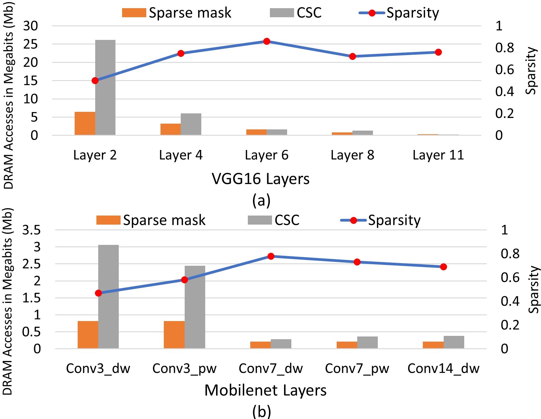
Figure 25. Sparse mask vs. CSC DRAM access for (a) VGG16 (b) MobileNet

Comparing different versions of the Phantom-2D accelerators, Phantom-2D-HP, on average, offers $108.9\%$ and $27.4\%$ increase in speedup over Phantom-2D-CV and Phantom-2D-MD, respectively, for sparse MobileNet.

Comparing energy among different accelerators is quite challenging as it requires working RTLs. The energy consumption of an accelerator is dominated by the DRAM accesses, therefore, by estimating the DRAM accesses, energy difference among the accelerators can be approximated. Since many of the recent works rely on the CSC format for non-zero data storage, we compare the accessed memory for the CSC format against the sparse mask format. Figure 25 shows the intermediate activations’ memory access comparison for selected VGG 16 and MobileNet layers . The activation sparsity for different layers is also shown. In the initial layers with low activation sparsity, the CSC format has approximately $4\times$ and $3.7\times$ higher DRAM memory accesses than the sparse mask for VGG16 and Mobilenet, respectively. In the deeper layers with moderate to high sparsity, the memory requirement for the CSC format is around $1.7\times$ that of the sparse mask.

This shows that the sparse mask representation not only needs less encoding/decoding logic, but is also efficient in terms of memory requirements when compared against the CSC format. This translates directly to higher energy, area, and compute savings for the accelerators employing the sparse mask format.

5.2.5. RTL Synthesis Results

We wrote the RTL Verilog for a single Phantom core with $L_{f}=27$ (high performance) and synthesized it for the Xilinx Zynq 7100 SoC’s programmable logic (PL), running at 150 MHz. The SoC’s ARM-based processing system (PS) was used to transfer data to/from a desktop computer to DRAM. The PL acquires this data and stores it in its global buffers (input and weight SRAMs), shown in Figure 14. The generated outputs and the sparse masks are stored in the output SRAMs and transferred to DRAM for the next layer. Table 3 shows the total resource utilization among various sub-blocks of the Phantom core. The main takeaway is that the novel components of the Phantom core (LAM, TDS, Mapper, and intra-core balancer) only account for approximately 48% and 35% of the utilized LUT and the FF cost, respectively. The local SRAM utilization is dominated by the mapper and the output buffering block (approximately 78%). The design has a power consumption of 2.48W with the PS dominating the consumption (55%). Eyeriss v2, implemented on a 65nm ASIC, utilizes 2695k gates which represents a 108% increase in area cost when compared to the original semi-sparse Eyeriss (Chen et al., 2017). This drastic increase in area is the result of the complex encoding/decoding logic required by the CSC format in their design. SCNN has a 35% increase in area compared to their dense design, whereas, SparTen does not report the resource utilization of their PEs.

Table 3. Resource utilization for a single Phantom core with $L_{f}=27$

Property	Available	Used	Utilization (%)
LUTs	277k	3.4k	$1.23\%$
FFs	554k	6k	$1.1\%$
On-chip SRAM	26.5Mb	2.1kB	$0.01\%$

6. Conclusion

Designing a CNN accelerator to leverage the two-sided sparsity is quite challenging owing to the varying layer shapes and sizes, associated with a sparse model. In this paper, we have introduced Phantom: a novel multi-threaded, flexible, neural computational core that exploits the two-sided sparsity to provide high gains in performance at a relatively low hardware complexity. Using a system of Phantom cores, we then design the Phantom-2D accelerator, and present a novel dataflow that efficiently uses the capabilities of the Phantom cores. As opposed to many previous approaches, the Phantom-2D accelerator supports all layers of a CNN, including unit and non-unit stride convolutions, and FC layers. In addition, we have also proposed a two-level load balancing strategy that efficiently balances the load across the architecture level (inter-core), and at the thread level (intra-core) to minimize idling of the compute threads, thereby, further increasing the throughput. We have also performed comparisons against many previous state-of-the-art two-sided sparse CNN accelerators. Our simulations show that, on average, Phantom-2D accelerator performs $12\times$, $4.1\times$, $1.98\times$, and $2.36\times$, better than an equivalent dense CNN architecture, SCNN, SparTen, and Eyeriss v2, respectively, while retaining the energy efficiency of SparTen.

References

- (1)
- Albericio et al. (2016) J. Albericio, P. Judd, T. Hetherington, T. Aamodt, N. E. Jerger, and A. Moshovos. 2016. Cnvlutin: Ineffectual-Neuron-Free Deep Neural Network Computing. In 2016 ACM/IEEE 43rd Annual International Symposium on Computer Architecture (ISCA). 1–13. https://doi.org/10.1109/ISCA.2016.11
- Alwani et al. (2016) M. Alwani, H. Chen, M. Ferdman, and P. Milder. 2016. Fused-layer CNN accelerators. In 2016 49th Annual IEEE/ACM International Symposium on Microarchitecture (MICRO). 1–12. https://doi.org/10.1109/MICRO.2016.7783725
- Ankit et al. (2019) Aayush Ankit, Izzat El Hajj, Sai Rahul Chalamalasetti, Geoffrey Ndu, Martin Foltin, R. Stanley Williams, Paolo Faraboschi, Wen mei Hwu, John Paul Strachan, Kaushik Roy, and Dejan S Milojicic. 2019. PUMA: A Programmable Ultra-efficient Memristor-based Accelerator for Machine Learning Inference. arXiv:1901.10351 [cs.ET]
- Bai et al. (2018) L. Bai, Y. Zhao, and X. Huang. 2018. A CNN Accelerator on FPGA Using Depthwise Separable Convolution. IEEE Transactions on Circuits and Systems II: Express Briefs 65, 10 (2018), 1415–1419.
- Baştürk et al. (2017) Alper Baştürk, Mehmet Emin Yüksei, Hasan Badem, and Abdullah Çalışkan. 2017. Deep neural network based diagnosis system for melanoma skin cancer. In 2017 25th Signal Processing and Communications Applications Conference (SIU). 1–4. https://doi.org/10.1109/SIU.2017.7960563
- Bi et al. (2018) Xia-an Bi, Yingchao Liu, Qin Jiang, Qing Shu, Qi Sun, and Jianhua Dai. 2018. The Diagnosis of Autism Spectrum Disorder Based on the Random Neural Network Cluster. Frontiers in Human Neuroscience 12 (2018), 257. https://doi.org/10.3389/fnhum.2018.00257
- Chang and Chang (2020) K. Chang and T. Chang. 2020. VWA: Hardware Efficient Vectorwise Accelerator for Convolutional Neural Network. IEEE Transactions on Circuits and Systems I: Regular Papers 67, 1 (2020), 145–154.
- Chen et al. (2017) Y. Chen, T. Krishna, J. S. Emer, and V. Sze. 2017. Eyeriss: An Energy-Efficient Reconfigurable Accelerator for Deep Convolutional Neural Networks. IEEE Journal of Solid-State Circuits 52, 1 (2017), 127–138.
- Chen et al. (2019) Y. Chen, T. Yang, J. Emer, and V. Sze. 2019. Eyeriss v2: A Flexible Accelerator for Emerging Deep Neural Networks on Mobile Devices. IEEE Journal on Emerging and Selected Topics in Circuits and Systems 9, 2 (2019), 292–308. https://doi.org/10.1109/JETCAS.2019.2910232
- Collobert et al. (2011) Ronan Collobert, Jason Weston, Leon Bottou, Michael Karlen, Koray Kavukcuoglu, and Pavel Kuksa. 2011. Natural Language Processing (Almost) from Scratch. Journal of Machine Learning Research 12 (02 2011), 2493–2537.
- Delmas et al. (2018) Alberto Delmas, Patrick Judd, Dylan Malone Stuart, Zissis Poulos, Mostafa Mahmoud, Sayeh Sharify, Milos Nikolic, and Andreas Moshovos. 2018. Bit-Tactical: Exploiting Ineffectual Computations in Convolutional Neural Networks: Which, Why, and How. arXiv:1803.03688 [cs.NE]
- Ding et al. (2017) C. Ding, S. Liao, Y. Wang, Z. Li, N. Liu, Y. Zhuo, C. Wang, X. Qian, Y. Bai, G. Yuan, X. Ma, Y. Zhang, J. Tang, Q. Qiu, X. Lin, and B. Yuan. 2017. CirCNN: Accelerating and Compressing Deep Neural Networks Using Block-Circulant Weight Matrices. In 2017 50th Annual IEEE/ACM International Symposium on Microarchitecture (MICRO). 395–408.
- Du et al. (2015) Z. Du, R. Fasthuber, T. Chen, P. Ienne, L. Li, T. Luo, X. Feng, Y. Chen, and O. Temam. 2015. ShiDianNao: Shifting vision processing closer to the sensor. In 2015 ACM/IEEE 42nd Annual International Symposium on Computer Architecture (ISCA). 92–104. https://doi.org/10.1145/2749469.2750389
- Gokhale et al. (2017) V. Gokhale, A. Zaidy, A. X. M. Chang, and E. Culurciello. 2017. Snowflake: An efficient hardware accelerator for convolutional neural networks. In 2017 IEEE International Symposium on Circuits and Systems (ISCAS). 1–4. https://doi.org/10.1109/ISCAS.2017.8050809
- Gondimalla et al. (2019) Ashish Gondimalla, Noah Chesnut, Mithuna Thottethodi, and T. N. Vijaykumar. 2019. SparTen: A Sparse Tensor Accelerator for Convolutional Neural Networks. In Proceedings of the 52nd Annual IEEE/ACM International Symposium on Microarchitecture (Columbus, OH, USA) (MICRO ’52). Association for Computing Machinery, New York, NY, USA, 151–165. https://doi.org/10.1145/3352460.3358291
- Guo et al. (2017) Xinyu Guo, Kelli C Dominick, A. Minai, Hailong Li, Craig A. Erickson, and Long Lu. 2017. Diagnosing Autism Spectrum Disorder from Brain Resting-State Functional Connectivity Patterns Using a Deep Neural Network with a Novel Feature Selection Method. Frontiers in Neuroscience 11 (2017).
- Gupta et al. (2015) Suyog Gupta, Ankur Agrawal, Kailash Gopalakrishnan, and Pritish Narayanan. 2015. Deep Learning with Limited Numerical Precision. arXiv:1502.02551 [cs.LG]
- Han et al. (2016) S. Han, X. Liu, H. Mao, J. Pu, A. Pedram, M. A. Horowitz, and W. J. Dally. 2016. EIE: Efficient Inference Engine on Compressed Deep Neural Network. In 2016 ACM/IEEE 43rd Annual International Symposium on Computer Architecture (ISCA). 243–254. https://doi.org/10.1109/ISCA.2016.30
- Han et al. (2016) Song Han, Huizi Mao, and William J. Dally. 2016. Deep Compression: Compressing Deep Neural Networks with Pruning, Trained Quantization and Huffman Coding. arXiv:1510.00149 [cs.CV]
- He et al. (2015) Kaiming He, Xiangyu Zhang, Shaoqing Ren, and Jian Sun. 2015. Deep Residual Learning for Image Recognition. arXiv:1512.03385 [cs.CV]
- Hegde et al. (2019) Kartik Hegde, Hadi Asghari-Moghaddam, Michael Pellauer, Neal Crago, Aamer Jaleel, Edgar Solomonik, Joel Emer, and Christopher W. Fletcher. 2019. ExTensor: An Accelerator for Sparse Tensor Algebra. In Proceedings of the 52nd Annual IEEE/ACM International Symposium on Microarchitecture (Columbus, OH, USA) (MICRO ’52). Association for Computing Machinery, New York, NY, USA, 319–333. https://doi.org/10.1145/3352460.3358275
- Hinton et al. (2012) Geoffrey Hinton, Li Deng, Dong Yu, George E. Dahl, Abdel-rahman Mohamed, Navdeep Jaitly, Andrew Senior, Vincent Vanhoucke, Patrick Nguyen, Tara N. Sainath, and Brian Kingsbury. 2012. Deep Neural Networks for Acoustic Modeling in Speech Recognition: The Shared Views of Four Research Groups. IEEE Signal Processing Magazine 29, 6 (2012), 82–97. https://doi.org/10.1109/MSP.2012.2205597
- Horowitz (2014) Mark Horowitz. 2014. 1.1 Computing’s energy problem (and what we can do about it). Digest of Technical Papers - IEEE International Solid-State Circuits Conference 57, 10–14. https://doi.org/10.1109/ISSCC.2014.6757323
- Howard et al. (2017) Andrew G. Howard, Menglong Zhu, Bo Chen, Dmitry Kalenichenko, Weijun Wang, Tobias Weyand, Marco Andreetto, and Hartwig Adam. 2017. MobileNets: Efficient Convolutional Neural Networks for Mobile Vision Applications. arXiv:1704.04861 [cs.CV]
- Jouppi et al. (2017) Norman P. Jouppi, Cliff Young, Nishant Patil, David Patterson, Gaurav Agrawal, Raminder Bajwa, Sarah Bates, Suresh Bhatia, Nan Boden, Al Borchers, Rick Boyle, Pierre luc Cantin, Clifford Chao, Chris Clark, Jeremy Coriell, Mike Daley, Matt Dau, Jeffrey Dean, Ben Gelb, Tara Vazir Ghaemmaghami, Rajendra Gottipati, William Gulland, Robert Hagmann, C. Richard Ho, Doug Hogberg, John Hu, Robert Hundt, Dan Hurt, Julian Ibarz, Aaron Jaffey, Alek Jaworski, Alexander Kaplan, Harshit Khaitan, Andy Koch, Naveen Kumar, Steve Lacy, James Laudon, James Law, Diemthu Le, Chris Leary, Zhuyuan Liu, Kyle Lucke, Alan Lundin, Gordon MacKean, Adriana Maggiore, Maire Mahony, Kieran Miller, Rahul Nagarajan, Ravi Narayanaswami, Ray Ni, Kathy Nix, Thomas Norrie, Mark Omernick, Narayana Penukonda, Andy Phelps, Jonathan Ross, Matt Ross, Amir Salek, Emad Samadiani, Chris Severn, Gregory Sizikov, Matthew Snelham, Jed Souter, Dan Steinberg, Andy Swing, Mercedes Tan, Gregory Thorson, Bo Tian, Horia Toma, Erick Tuttle, Vijay Vasudevan, Richard Walter, Walter Wang, Eric Wilcox, and Doe Hyun Yoon. 2017. In-Datacenter Performance Analysis of a Tensor Processing Unit. arXiv:1704.04760 [cs.AR]
- Judd et al. (2016) Patrick Judd, Jorge Albericio, Tayler Hetherington, Tor M. Aamodt, and Andreas Moshovos. 2016. Stripes: Bit-Serial Deep Neural Network Computing. In The 49th Annual IEEE/ACM International Symposium on Microarchitecture (Taipei, Taiwan) (MICRO-49). IEEE Press, Article 19, 12 pages.
- Krizhevsky et al. (2012) Alex Krizhevsky, Ilya Sutskever, and Geoffrey E. Hinton. 2012. ImageNet Classification with Deep Convolutional Neural Networks. In Proceedings of the 25th International Conference on Neural Information Processing Systems - Volume 1 (Lake Tahoe, Nevada) (NIPS’12). Curran Associates Inc., Red Hook, NY, USA, 1097–1105.
- Le Cun et al. (1989) Y. Le Cun, L.D. Jackel, B. Boser, J.S. Denker, H.P. Graf, I. Guyon, D. Henderson, R.E. Howard, and W. Hubbard. 1989. Handwritten digit recognition: applications of neural network chips and automatic learning. IEEE Communications Magazine 27, 11 (1989), 41–46. https://doi.org/10.1109/35.41400
- Lee et al. (2018) Jinmook Lee, Changhyeon Kim, Sanghoon Kang, Dongjoo Shin, Sangyeob Kim, and Hoi-Jun Yoo. 2018. UNPU: An energy-efficient deep neural network accelerator with fully variable weight bit precision. IEEE Journal of Solid-State Circuits 54, 1 (2018), 173–185.
- Lin et al. (2016) Darryl D. Lin, Sachin S. Talathi, and V. Sreekanth Annapureddy. 2016. Fixed Point Quantization of Deep Convolutional Networks. arXiv:1511.06393 [cs.LG]
- Liu et al. (2019) Bing Liu, Danyin Zou, Lei Feng, Shou Feng, Ping Fu, and Junbao Li. 2019. An FPGA-based CNN accelerator integrating depthwise separable convolution. Electronics 8, 3 (2019), 281.
- Liu et al. (2015) Daofu Liu, Tianshi Chen, Shaoli Liu, Jinhong Zhou, Shengyuan Zhou, Olivier Teman, Xiaobing Feng, Xuehai Zhou, and Yunji Chen. 2015. PuDianNao: A Polyvalent Machine Learning Accelerator. SIGPLAN Not. 50, 4 (March 2015), 369–381. https://doi.org/10.1145/2775054.2694358
- Miao et al. (2021) Yuantian Miao, Chao Chen, Lei Pan, Qing-Long Han, Jun Zhang, and Yang Xiang. 2021. Machine Learning Based Cyber Attacks Targeting on Controlled Information: A Survey. arXiv:2102.07969 [cs.CR]
- Mirsky et al. (2021) Yisroel Mirsky, Ambra Demontis, Jaidip Kotak, Ram Shankar, Deng Gelei, Liu Yang, Xiangyu Zhang, Wenke Lee, Yuval Elovici, and Battista Biggio. 2021. The Threat of Offensive AI to Organizations. arXiv:2106.15764 [cs.AI]
- Miyashita et al. (2016) Daisuke Miyashita, Edward H. Lee, and Boris Murmann. 2016. Convolutional Neural Networks using Logarithmic Data Representation. arXiv:1603.01025 [cs.NE]
- Moons et al. (2017) Bert Moons, Roel Uytterhoeven, Wim Dehaene, and Marian Verhelst. 2017. 14.5 envision: A 0.26-to-10tops/w subword-parallel dynamic-voltage-accuracy-frequency-scalable convolutional neural network processor in 28nm fdsoi. In 2017 IEEE International Solid-State Circuits Conference (ISSCC). IEEE, 246–247.
- Mursi et al. (2020) Khalid T. Mursi, Bipana Thapaliya, Yu Zhuang, Ahmad O. Aseeri, and Mohammed Saeed Alkatheiri. 2020. A Fast Deep Learning Method for Security Vulnerability Study of XOR PUFs. Electronics 9, 10 (2020). https://doi.org/10.3390/electronics9101715
- Pal et al. (2018) Subhankar Pal, Jonathan Beaumont, Dong-Hyeon Park, Aporva Amarnath, Siying Feng, Chaitali Chakrabarti, Hun-Seok Kim, David Blaauw, Trevor Mudge, and Ronald Dreslinski. 2018. OuterSPACE: An Outer Product Based Sparse Matrix Multiplication Accelerator. In 2018 IEEE International Symposium on High Performance Computer Architecture (HPCA). 724–736. https://doi.org/10.1109/HPCA.2018.00067
- Parashar et al. (2017) A. Parashar, M. Rhu, A. Mukkara, A. Puglielli, R. Venkatesan, B. Khailany, J. Emer, S. W. Keckler, and W. J. Dally. 2017. SCNN: An accelerator for compressed-sparse convolutional neural networks. In 2017 ACM/IEEE 44th Annual International Symposium on Computer Architecture (ISCA). 27–40. https://doi.org/10.1145/3079856.3080254
- Qin et al. (2020) Eric Qin, Ananda Samajdar, Hyoukjun Kwon, Vineet Nadella, Sudarshan Srinivasan, Dipankar Das, Bharat Kaul, and Tushar Krishna. 2020. SIGMA: A Sparse and Irregular GEMM Accelerator with Flexible Interconnects for DNN Training. In 2020 IEEE International Symposium on High Performance Computer Architecture (HPCA). 58–70. https://doi.org/10.1109/HPCA47549.2020.00015
- Qureshi and Munir (2019) Mahmood Azhar Qureshi and Arslan Munir. 2019. PUF-RLA: A PUF-Based Reliable and Lightweight Authentication Protocol Employing Binary String Shuffling. In 2019 IEEE 37th International Conference on Computer Design (ICCD). 576–584. https://doi.org/10.1109/ICCD46524.2019.00084
- Qureshi and Munir (2020a) Mahmood Azhar Qureshi and Arslan Munir. 2020a. NeuroMAX: A High Throughput, Multi-Threaded, Log-Based Accelerator for Convolutional Neural Networks. In 2020 IEEE/ACM International Conference On Computer Aided Design (ICCAD). 1–9.
- Qureshi and Munir (2020b) Mahmood Azhar Qureshi and Arslan Munir. 2020b. PUF-IPA: A PUF-based Identity Preserving Protocol for Internet of Things Authentication. In 2020 IEEE 17th Annual Consumer Communications Networking Conference (CCNC). 1–7. https://doi.org/10.1109/CCNC46108.2020.9045264
- Qureshi and Munir (2021a) Mahmood Azhar Qureshi and Arslan Munir. 2021a. PUF-RAKE: A PUF-based Robust and Lightweight Authentication and Key Establishment Protocol. IEEE Transactions on Dependable and Secure Computing (2021), 1–1. https://doi.org/10.1109/TDSC.2021.3059454
- Qureshi and Munir (2021b) Mahmood Azhar Qureshi and Arslan Munir. 2021b. Sparse-PE: A Performance-Efficient Processing Engine Core for Sparse Convolutional Neural Networks. IEEE Access (2021), 1–1. https://doi.org/10.1109/ACCESS.2021.3126708
- Sandler et al. (2018) Mark Sandler, Andrew Howard, Menglong Zhu, Andrey Zhmoginov, and Liang-Chieh Chen. 2018. MobileNetV2: Inverted Residuals and Linear Bottlenecks. arXiv:1801.04381 [cs.CV]
- Santikellur et al. (2019) Pranesh Santikellur, Aritra Bhattacharyay, and Rajat Subhra Chakraborty. 2019. Deep Learning based Model Building Attacks on Arbiter PUF Compositions. IACR Cryptol. ePrint Arch. 2019 (2019), 566.
- Shafiee et al. (2016) A. Shafiee, A. Nag, N. Muralimanohar, R. Balasubramonian, J. P. Strachan, M. Hu, R. S. Williams, and V. Srikumar. 2016. ISAAC: A Convolutional Neural Network Accelerator with In-Situ Analog Arithmetic in Crossbars. In 2016 ACM/IEEE 43rd Annual International Symposium on Computer Architecture (ISCA). 14–26. https://doi.org/10.1109/ISCA.2016.12
- Sharify et al. (2019) Sayeh Sharify, Alberto Delmas Lascorz, Mostafa Mahmoud, Milos Nikolic, Kevin Siu, Dylan Malone Stuart, Zissis Poulos, and Andreas Moshovos. 2019. Laconic Deep Learning Inference Acceleration. In Proceedings of the 46th International Symposium on Computer Architecture (Phoenix, Arizona) (ISCA ’19). Association for Computing Machinery, New York, NY, USA, 304–317. https://doi.org/10.1145/3307650.3322255
- Siar and Teshnehlab (2019) Masoumeh Siar and Mohammad Teshnehlab. 2019. Brain Tumor Detection Using Deep Neural Network and Machine Learning Algorithm. In 2019 9th International Conference on Computer and Knowledge Engineering (ICCKE). 363–368. https://doi.org/10.1109/ICCKE48569.2019.8964846
- Simonyan and Zisserman (2014) Karen Simonyan and Andrew Zisserman. 2014. Very Deep Convolutional Networks for Large-Scale Image Recognition. arXiv:1409.1556 [cs.CV]
- Srivastava et al. (2020a) Nitish Srivastava, Hanchen Jin, Jie Liu, David Albonesi, and Zhiru Zhang. 2020a. MatRaptor: A Sparse-Sparse Matrix Multiplication Accelerator Based on Row-Wise Product. In 2020 53rd Annual IEEE/ACM International Symposium on Microarchitecture (MICRO). 766–780. https://doi.org/10.1109/MICRO50266.2020.00068
- Srivastava et al. (2020b) Nitish Srivastava, Hanchen Jin, Shaden Smith, Hongbo Rong, David Albonesi, and Zhiru Zhang. 2020b. Tensaurus: A Versatile Accelerator for Mixed Sparse-Dense Tensor Computations. In 2020 IEEE International Symposium on High Performance Computer Architecture (HPCA). 689–702. https://doi.org/10.1109/HPCA47549.2020.00062
- Sze et al. (2017) V. Sze, Y. Chen, T. Yang, and J. S. Emer. 2017. Efficient Processing of Deep Neural Networks: A Tutorial and Survey. Proc. IEEE 105, 12 (2017), 2295–2329.
- Szegedy et al. (2015) Christian Szegedy, Wei Liu, Yangqing Jia, Pierre Sermanet, Scott Reed, Dragomir Anguelov, Dumitru Erhan, Vincent Vanhoucke, and Andrew Rabinovich. 2015. Going Deeper with Convolutions. In Computer Vision and Pattern Recognition (CVPR). http://arxiv.org/abs/1409.4842
- Tan and Le (2021) Mingxing Tan and Quoc V. Le. 2021. EfficientNetV2: Smaller Models and Faster Training. arXiv:2104.00298 [cs.CV]
- van den Oord et al. (2016) Aäron van den Oord, Sander Dieleman, Heiga Zen, Karen Simonyan, Oriol Vinyals, Alex Graves, Nal Kalchbrenner, Andrew W. Senior, and Koray Kavukcuoglu. 2016. WaveNet: A Generative Model for Raw Audio. CoRR abs/1609.03499 (2016). arXiv:1609.03499 http://arxiv.org/abs/1609.03499
- Vogel et al. (2018) Sebastian Vogel, Mengyu Liang, Andre Guntoro, Walter Stechele, and Gerd Ascheid. 2018. Efficient Hardware Acceleration of CNNs Using Logarithmic Data Representation with Arbitrary Log-Base. In Proceedings of the International Conference on Computer-Aided Design (San Diego, California) (ICCAD ’18). Association for Computing Machinery, New York, NY, USA, Article 9, 8 pages. https://doi.org/10.1145/3240765.3240803
- Wu et al. (2016) Yonghui Wu, Mike Schuster, Zhifeng Chen, Quoc V. Le, Mohammad Norouzi, Wolfgang Macherey, Maxim Krikun, Yuan Cao, Qin Gao, Klaus Macherey, Jeff Klingner, Apurva Shah, Melvin Johnson, Xiaobing Liu, Łukasz Kaiser, Stephan Gouws, Yoshikiyo Kato, Taku Kudo, Hideto Kazawa, Keith Stevens, George Kurian, Nishant Patil, Wei Wang, Cliff Young, Jason Smith, Jason Riesa, Alex Rudnick, Oriol Vinyals, Greg Corrado, Macduff Hughes, and Jeffrey Dean. 2016. Google’s Neural Machine Translation System: Bridging the Gap between Human and Machine Translation. arXiv:1609.08144 [cs.CL]
- Zhang et al. (2016) S. Zhang, Z. Du, L. Zhang, H. Lan, S. Liu, L. Li, Q. Guo, T. Chen, and Y. Chen. 2016. Cambricon-X: An accelerator for sparse neural networks. In 2016 49th Annual IEEE/ACM International Symposium on Microarchitecture (MICRO). 1–12. https://doi.org/10.1109/MICRO.2016.7783723
- Zhang et al. (2020) Zhekai Zhang, Hanrui Wang, Song Han, and William J. Dally. 2020. SpArch: Efficient Architecture for Sparse Matrix Multiplication. In 2020 IEEE International Symposium on High Performance Computer Architecture (HPCA). 261–274. https://doi.org/10.1109/HPCA47549.2020.00030
- Zhou et al. (2018) Xuda Zhou, Zidong Du, Qi Guo, Shaoli Liu, Chengsi Liu, Chao Wang, Xuehai Zhou, Ling Li, Tianshi Chen, and Yunji Chen. 2018. Cambricon-s: Addressing Irregularity in Sparse Neural Networks through a Cooperative Software/Hardware Approach. In Proceedings of the 51st Annual IEEE/ACM International Symposium on Microarchitecture (Fukuoka, Japan) (MICRO-51). IEEE Press, 15–28. https://doi.org/10.1109/MICRO.2018.00011