Parameterized complexity of untangling knots

Abstract

Deciding whether a diagram of a knot can be untangled with a given number of moves (as a part of the input) is known to be NP-complete. In this paper we determine the parameterized complexity of this problem with respect to a natural parameter called defect. Roughly speaking, it measures the efficiency of the moves used in the shortest untangling sequence of Reidemeister moves.

We show that the $\rm{II}^{-}$ moves in a shortest untangling sequence can be essentially performed greedily. Using that, we show that this problem belongs to W[P] when parameterized by the defect. We also show that this problem is W[P]-hard by a reduction from Minimum axiom set.

1 Introduction

A classical and extensively studied question in algorithmic knot theory is to determine whether a given diagram of a knot is actually a diagram of an unknot. This question is known as the unknot recognition problem. The first algorithm for this problem was given by Haken [Hak61]. Currently, it is known that the unknot recognition problem belongs to NP$\,\cap\,$co-NP but no polynomial time algorithm is known. See [HLP99] for the NP-membership and [Lac16] for co-NP-membership (co-NP-membership modulo Generalized Riemann Hypothesis was previously established in [Kup14]). In addition, a quasi-polynomial time algorithm for unknot recognition has been recently announced by Lackenby [Lac21].

One possible path for attacking the unknot recognition problem is via Reidemeister moves (see Figure 2): if $D$ is a diagram of an unknot, then $D$ can be untangled to a diagram $U$ with no crossing by a finite number of Reidemeister moves. In addition, Lackenby [Lac15] provided a polynomial bound (in the number of crossings of $D$) on the required number of Reidemeister moves. This is an alternative way to show that the unknot recognition problem belongs to NP, because it is sufficient to guess the required Reidemeister moves for unknotting.

However, if we slightly change our viewpoint, de Mesmay, Rieck, Sedgwick, and Tancer [dMRST21] showed that it is NP-hard to count the number of required Reidemeister moves exactly. (An anologous result for links has been shown to be NP-hard slightly earlier by Koenig and Tsvietkova [KT21].) More precisely, it is shown in [dMRST21] that given a digram $D$ and a parameter $k$ as input, it is NP-hard to decide whether $D$ can be untangled using at most $k$ Reidemeiser moves. For more background on unknotting and unlinking problems, we also refer to Lackenby’s survey [Lac17].

The main aim of this paper is to extend the line of research started in [dMRST21] by determining the parameterized complexity of untangling knots via Reidemeister moves. On the one hand, it is easy to see that if we consider parameterization by the number of Reidemeister moves, then the problem is in FPT (class of fixed parameter tractable problems). This happens because of a somewhat trivial reason: if a diagram $D$ can be untangled with at most $k$ moves, then $D$ contains at most $2k$ crossings, thus we can assume that the size of $D$ is (polynomially) bounded by $k$. On the other hand, we also consider parameterization with an arguably much more natural parameter called the defect (used in [dMRST21]). This parameterization is also relevant from the point of view of above guarantee parameterization introduced by Mahajan and Raman [MR99]. Here we show that the problem is W[P]-complete with respect to this parameter. This is the core of the paper.

In order to state our results more precisely, we need a few preliminaries on diagrams and Reidemeister moves. For purposes of this part of the introduction, we also assume that the reader is at least briefly familiar with complexity classes FPT and W[P]. Otherwise we refer to Subsection 1.1 where we briefly overview these classes, and to the references in this subsection.

Diagrams and Reidemeister moves.

A diagram of a knot is a piecewise linear map $D\colon S^{1}\to{\mathbb{R}}^{2}$ in general position; for such a map, every point in ${\mathbb{R}}^{2}$ has at most two preimages, and there are finitely many points in ${\mathbb{R}}^{2}$ with exactly two preimages (called crossings). Locally at crossing two arcs cross each other transversely, and the diagram contains the information of which arc passes ‘over’ and which ‘under’. This we usually depict by interrupting the arc that passes under. (A diagram usually arises as a composition of a (piecewise linear) knot $\kappa\colon S^{1}\to{\mathbb{R}}^{3}$ and a generic projection $\pi\colon{\mathbb{R}}^{3}\to{\mathbb{R}}^{2}$ which also induces ‘over’ and ‘under’ information.) We usually identify a diagram $D$ with its image in ${\mathbb{R}}^{2}$ together with the information about underpasses/overpasses at crossings. Diagrams are always considered up-to isotopy. The unique diagram without crossings is denoted $U$ (untangled). See Figure 1 for an example of a diagram.

Figure 1: An example of a diagram.

Let $D$ be a diagram of a knot. Reidemeister moves are local modifications of the diagram depicted at Figure 2. We distinguish Reidemeister moves of types $\rm{I}$, $\rm{II}$, and $\rm{III}$ as depicted in the figure. In addition, for types $\rm{I}$ and $\rm{II}$, we distinguish whether the moves remove crossings (types $\rm{I}^{-}$ and $\rm{II}^{-}$) or whether they introduce new crossings (types $\rm{I}^{+}$ and ${\rm{II}^{+}}$).

Figure 2: Reidemeister moves

A diagram $D$ is a diagram of an unknot if it can be transformed to the untangled diagram $U$ by a finite sequence of Reidemeister moves. (This is well known to be equivalent to stating that the lift of the diagram to ${\mathbb{R}}^{3}$, keeping the underpasses/overpasses is ambient isotopic to the unknot, that is standardly embedded $S^{1}$ in ${\mathbb{R}}^{3}$.) The diagram on Figure 1 is a diagram of an unknot.

Now we discuss different parameterizations of untangling (un)knots via Reidemeister moves in more detail.

Parameterization via number of Reidemeister moves.

In the first case, we consider the following parameterized problem.

Problem (Unknotting via number of moves).

Input	A diagram $D$ of a knot.
Parameter	$k$.
Question	Can $D$ be untangled to an unknot using at most $k$ Reidemeister moves?

Observation 1.

Unknotting via number of moves belongs to FPT.

Sketch.

Each Reidemeister move removes at most $2$ crossings. Thus, if $D$ contains at least $2k+1$ crossings, then we immediately answer No. This can be determined in time $O(|D|)$, where $|D|$ stands for the size of the encoding of $D$.

It remains to resolve the case when $D$ contains at most $2k$ crossings. In this case we perform the naive algorithm trying all possible sequences of Reidemeister moves. We will see that if $D$ has $n$ crossings, then there are at most $O(n^{2})$ feasible Reidemeister moves—see Lemma 4 (a more naive analysis yields $O(n^{3})$). Each of them can be performed in time $O(n\log n)$—see Lemma 4 again. In addition, any diagram obtained after performing a Reidemeister move on $D$ has at most $n+2$ crossings. This gives that all feasible sequences of at most $k$ Reidemeister moves starting with $D$ can be constructed and performed in time $O(k^{2k+2}\log k)$. Indeed, each such sequence can be constructed and performed in time $O(k^{2}\log k)$ and there are at most $O(k^{2k})$ such sequences. If any of them yields a diagram without crossings, then we answer Yes, otherwise we answer No.

Altogether, Unknotting via number of moves can be solved in time $O(k^{2k+2}\log k)+O(|D|)$, therefore, it belongs to FPT. (Of course, in the sketch above, we didn’t really need to know the concrete bounds on the number of feasible Reidemeister moves and on the time for construction of all feasible sequences. Any computable function would have sufficed.) ∎

Parameterization via defect.

As we see from the sketch above, parameterization in the number of Reidemeister moves has the obvious disadvantage that once we fix $k$, the problem becomes trivial for arbitrarily large inputs (they are obviously a NO instance). We also see that if we have a diagram $D$ with $n$ crossings and want to minimize the number of Reidemeister moves to untangle $D$, presumably the most efficient way is to remove two crossings in each step, thus requiring at least $n/2$ steps. This motivates the following definition of the notion of defect.

Given a diagram $D$, by an untangling of $D$ we mean a sequence ${\mathcal{D}}=(D_{0},\dots,D_{\ell})$ such that $D=D_{0}$; $D_{i+1}$ is obtained from $D_{i}$ by a Reidemeister move; and $D_{\ell}=U$ is the diagram with no crossings. Then we define the defect of an untangling ${\mathcal{D}}$ as above as

$$\operatorname{def}({\mathcal{D}}):=2\ell-n$$

where $n$ is the number of crossings in $D$. Note that $\ell$ is just the number of Reidemeister moves in the untangling. It is easy to see that $\operatorname{def}({\mathcal{D}})\geq 0$ and $\operatorname{def}({\mathcal{D}})=0$ if and only if all moves in the untangling are $\rm{II}^{-}$ moves. Therefore, $\operatorname{def}({\mathcal{D}})$ in some sense measures the number of ‘extra’ moves in the untangling beyond the trivial bound. (Perhaps, a more accurate expression for this interpretation would be $\ell-n/2=\frac{1}{2}\operatorname{def}({\mathcal{D}})$ but this is a minor detail and it is more convenient to work with integers.) In addition, it is possible to get diagrams with arbitrarily large number of crossings but with defect bounded by a constant (even for defect $0$ this is possible). The defect also plays a key role in the reduction in [dMRST21] which suggests that the hardness of the untangling really depends on the defect.

As we have seen above, asking the question whether a diagram can be untangled with defect at most $k$ is same as asking if it can be untangled in $k/2$ moves above the trivial, but tight lower bound of $n/2$. This fits perfectly in the framework of above guarantee parameterization, which was introduced by Mahajan and Raman [MR99] for Max-Sat and Max-Cut problems. In this framework, when there is a trivial lower bound for the solution in terms of the size of the input, parameterizing by solution size trivially gives an FPT algorithm by either giving a trivial answer if the input is large, or bounding size of the input by a function of the solution size. Hence, for those problems, it makes more sense to parameterize above a tight lower bound. The paradigm of above guarantee parameterization has been very successful in the field of parameterized complexity and many results have been obtained [AGK⁺11, CFG⁺14, CJM⁺13, GKLM11, GvIMY12, GP16, MRS09].

For these reasons, we find the defect to be a more natural parameter than the number of Reidemeister moves. Therefore, we consider the following problem.

Problem (Unknotting via defect).

Input	A diagram $D$ of a knot.
Parameter	$k$.
Question	Can $D$ be untangled with defect at most $k$?

Theorem 2.

The problem Unknotting via defect is W[P]-complete.

The proof of Theorem 2 consists of two main steps: W[P]-membership and W[P]-hardness. Both of them are non-trivial.

For W[P]-membership, roughly speaking, the idea is to guess a small enough set of special crossings on which we perform all possible Reidemeister moves, while we remove other crossings in a greedy fashion. In order to succeed with such an approach we will need some powerful and flexible enough lemmas on changing the ordering of Reidemeister moves in some untangling by swapping them. In Subsection 1.2 we provide an algorithm for W[P]-membership but we do not prove yet that it works. Then we start filling in the details. In Section 2, we explain how we represent diagrams as an input for the algorithm. In Section 3 we explain how we implement Reidemeister moves with respect to the aforementioned representation of diagrams and also introduce some combinatorial notation for them which will be useful in further considerations. We also explain the idea of special crossings in detail and we provide a bound on the number of required special crossings with respect to the defect. In Section 4 we prove the correctness of our algorithm modulo a result on rearranging the moves, whose proof is postponed to Section 5.

For W[P]-hardness, we combine some techniques that were quite recently used in showing parameterized hardness of problems in computational topology [BLPS16, BRS19], along with the tools in [dMRST21] for lower bounding the defect. Namely, we use a reduction from the Minimum axiom set problem, which proved to be useful in [BLPS16, BRS19]. Roughly speaking, from an instance $I$ of the Minimum axiom set problem (which we have not defined yet), we need to build a diagram which has a small defect if and only if $I$ admits a small set of axioms. For the “if” part, we use properties of Brunnian rings to achieve our goal. For the “only if” part, we need to lower bound the defect of our construction. We use the tools from [dMRST21] to show that the defect (of some subinstances) is at least $1$. Then we use very simple but powerful boosting lemma (Lemma 15) that shows that the defect is actually high. We give the details of the hardness proof in Section 6.

We conclude this part of introduction by proving a lemma on the properties of the defect which we will use soon after.

Given a Reidemeister move $m$, let us define the weight of this move $w(m)$ as

$$w(m)=\left\{\begin{array}[]{ll}0&\mbox{if $m$ is a $\rm{II}^{-}$ move};\\ 1&\mbox{if $m$ is a $\rm{I}^{-}$ move};\\ 2&\mbox{if $m$ is a $\rm{III}$ move};\\ 3&\mbox{if $m$ is a $\rm{I}^{+}$ move};\\ 4&\mbox{if $m$ is a ${\rm{II}^{+}}$ move}.\\ \end{array}\right.$$

Lemma 3.

Let ${\mathcal{D}}$ be an untangling of a diagram $D$. Then $\operatorname{def}({\mathcal{D}})$ equals to the sum of the weights of the Reidemeister moves in ${\mathcal{D}}$.

Because the proof of the lemma is short, we present it immediately.

Proof.

We will give a proof by induction in the number of moves used in ${\mathcal{D}}$. There is nothing to prove if there is no move in ${\mathcal{D}}$ (in particular, $D$ is already untangled in this case).

Otherwise, let ${\mathcal{D}}=(D_{0},\dots,D_{\ell})$ with $\ell\geq 1$. Let ${\mathcal{D}}^{\prime}=(D_{1},\dots,D_{\ell})$ and let $m_{1}$ be the Reidemeister move transforming $D_{0}$ to $D_{1}$. Let $\ell^{\prime}:=\ell-1$ be the number of moves in ${\mathcal{D}}^{\prime}$; $n$ be the number of crossings in $D_{0}$ and $n^{\prime}$ be the number of crossings in $D_{1}$. We get

$$\operatorname{def}({\mathcal{D}})-\operatorname{def}({\mathcal{D}}^{\prime})=2\ell-n-(2\ell^{\prime}-n^{\prime})=2+(n^{\prime}-n)=w(m_{1})$$

where the last equality follows from a very simple case analysis depending on the type of $m_{1}$. Because $\operatorname{def}({\mathcal{D}}^{\prime})$ is the sum of the weights of the remaining moves (by induction), we get the desired conclusion. ∎

1.1 A brief overview of the parameterized complexity classes

Here we briefly overview the notions from parameterized complexity needed for this paper. For further background, we refer the reader to monographs [FG06, DF13, CFK⁺15]. A parameterized problem is a language $L\subseteq\Sigma^{*}\times\mathbb{N}$, where $\Sigma^{*}$ is the set of strings over a finite alphabet $\Sigma$ and the input strings are of the form $(x,k)$. Here the integer $k$ is called the parameter. Note that parameterized problems are sometimes equivalently defined as a subset $P$ of $\Sigma^{*}$ and a polynomial-time computable function $\kappa$ called parameter. In subsequent parts of the paper, given an input for a parameterized problem, $n$ denotes the size of the input and $k$ denotes the value of the parameter on this input.

The classes FPT and XP.

A parameterized problem belongs to the class FPT (fixed parameter tractable) if it can be solved by a deterministic Turing machine in time $f(k)\cdot n^{c}$ where $c>0$ is some constant and $f(k)$ is some computable function of $k$. In other words, if we fix $k$, then the problem can be solved in polynomial time while the degree of the polynomial does not depend on $k$. This is, of course, sometimes not achievable and there is a wider class XP of problems, that can be solved in time $O(n^{f(k)})$ by a deterministic Turing machine. The problems in XP are still polynomial time solvable for fixed $k$, however, at the cost that the degree of the polynomial depends on $k$.

The class W[P].

Somewhere in between FPT and XP there is an interesting class W[P]. A parameterized problem belongs to the class W[P] if it can be solved by a nondeterministic Turing machine in time $h(k)\cdot n^{c}$ provided that this machine makes only $O(f(k)\log n)$ non-deterministic choices where $f(k),h(k)$ are computable functions and $c>0$ is some constant. Given an algorithm for some computational problem $\Pi$, we say that this algorithm is a W[P]-algorithm if it is represented by a Turing machine satisfying the conditions above.

It is obvious that a problem in FPT belongs to W[P]—we use the same algorithm with $0$ non-deterministic choices. On the other hand, given a W[P]-algorithm, it can be converted to a deterministic algorithm by trying all option for each non-deterministic choice. The running time of the new algorithm is $h(k)\cdot n^{c}\cdot(c^{\prime})^{O(f(k)\log n)}$ for some $c^{\prime}>0$ which can be easily manipulated into a formula showing XP-membership.

FPT-reduction.

Given two parameterized problems $\Pi$ and $\Pi^{\prime}$, we say that $\Pi$ reduces to $\Pi^{\prime}$ via an FPT-reduction if there exist computable functions $f\colon\Sigma^{*}\times\mathbb{N}\to\Sigma^{*}$ and $g\colon\Sigma^{*}\times\mathbb{N}\to\mathbb{N}$ such that

• $(x,k)\in\Pi$ if and only if $(f(x,k),g(x,k))\in\Pi^{\prime}$ for every $(x,k)\in\Sigma^{*}\times\mathbb{N}$;

• $g(x,k)\leq g^{\prime}(k)$ for some computable function $g^{\prime}$; and

• there exist a computable function $h$ and a fixed constant $c>0$ such that for all input string, $f(x,k)$ can be computed by a deterministic Turing-machine in $O(h(k)n^{c})$ steps.

Let us remark that here we use a definition of reduction consistent with [FG06, Definition 2.1] or [CFK⁺15, Definition 13.1]. On the other hand, some authors, e.g. [DF13, Definition 20.2.1], impose a stronger requirement that would correspond to asking $g(x,k)=g^{\prime}(k)$ in the second item of our definition. Thus our hardness claims are with respect to the reduction we define here.

The classes FPT, W[P] and XP are closed under FPT-reductions. A problem $\Pi$ is said to be C-hard where C is a parameterized complexity class, if all problems in C can be FPT-reduced to $\Pi$. Moreover, if $\Pi\in\hbox{C}$, we say that $\Pi$ is C-complete.

1.2 An algorithm for W[P]-membership

In this subsection we provide the algorithm used to prove W[P]-membership in Theorem 2.

Brute force algorithm.

First, let us however look at a brute force algorithm for Unknotting via defect which does not give W[P]-membership. Spelling it out will be useful for explaining the next steps. We will exhibit this algorithm as a non-deterministic algorithm, which will be useful for comparison later on. In the algorithm, $D$ is a diagram, and $k$ is an integer, not necessarily positive. Also, given a diagram $D$ and a feasible Reidemeister move $m$, then $D(m)$ denotes the diagram obtained from $D$ after performing $m$.

BruteForce$(D,k)$:

1. If $k<0$, then output No. If $D=U$ is a diagram without crossings and $k\geq 0$, then output Yes. In all other cases continue to the next step.

2. (Non-deterministic step.) Enumerate all possible Reidemeister moves $m_{1},\dots,m_{t}$ in $D$ up to isotopy. Make a ‘guess’ which move $m_{i}$ is the first to perform. Then, for such $m_{i}$, run BruteForce$(D(m_{i}),k-w(m_{i}))$.

Therefore, altogether, the algorithm outputs Yes, if there is a sequence of guesses in step 2 which eventually yields Yes in step 1.

It can be easily shown that the algorithm terminates because whenever step 2 is performed, either $k-w(m_{i})<k$, or $m_{i}$ is a $\rm{II}^{-}$ move, $k-w(m_{i})=k$, but $D(m_{i})$ has fewer crossings than $D$.

It can be also easily shown by induction that this algorithm provides a correct answer due to Lemma 3. Indeed, step 1 clearly provides a correct answer, and regarding step 2, if $D(m_{i})$ can be untangled with defect at most $k-w(m_{i})$, then Lemma 3 shows that $D$ can be untangled with defect at most $k$. Because, this way we try all possible sequences of Reidemeister moves, the algorithm outputs Yes if and only if $D$ can be untangled with defect at most $k$.

On the other hand, this algorithm (unsurprisingly) does not provide W[P]-membership as it performs too many non-deterministic guesses.

Naive greedy algorithm.

In order to fix the problem with the previous algorithm, we want to reduce the number of non-deteministic steps. It turns out that the problematic non-deterministic steps in the previous algorithm are those where $k$ does not decrease. (Because the other steps appear at most $k$ times.) Therefore, we want to avoid non-deterministic steps where we perform a $\rm{II}^{-}$ move. The naive way is to perform such steps greedily and hope that if $D$ untangles with defect at most $k$, there is also such a ‘greedy’ untangling (and therefore, we do not have to search through all possible sequences of Reidemeister moves). This is close to be true but it does not really work in this naive way. Anyway, we spell this naive algorithm explicitly, so that we can easily upgrade it in the next step, though it does not always provide the correct answer to Unknotting via defect.

NaiveGreedy$(D,k)$:

1. If $k<0$, then output No. If $D=U$ is a diagram without crossings and $k\geq 0$, then output Yes. In all other cases continue to the next step.

2. If there is a feasible Reidemeister $\rm{II}^{-}$ move $m$, run NaiveGreedy$(D(m),k)$ otherwise continue to the next step.

3. (Non-deterministic step.) If there is no feasible Reidemeister $\rm{II}^{-}$ move, enumerate all possible Reidemeister moves $m_{1},\dots,m_{t}$ in $D$ up to isotopy. Make a ‘guess’ which $m_{i}$ is the first move to perform and run NaiveGreedy$(D(m_{i}),k-w(m_{i}))$.

The algorithm must terminate from the same reason why BruteForce terminates.

It can be shown that this algorithm is a W[P]-algorithm. However, we do not do this here in detail as this is not our final algorithm. The key is that the step 3 is performed at most $(k+1)$-times.

If the algorithm outputs Yes, then this is clearly correct answer from the same reason as in the case of BruteForce. However, as we hinted earlier, outputting No need not be a correct answer to Unknotting via defect. Indeed, there are known examples of diagrams of an unknot when untangling requires performing a ${\rm{II}^{+}}$ move, see for example [KL12]. With NaiveGreedy, we would presumably undo such ${\rm{II}^{+}}$ move immediately in the next step, thus we would not find any untangling using the ${\rm{II}^{+}}$ move. We have to upgrade the algorithm a little bit to avoid this problem (and a few other similar problems).

Special greedy algorithm.

The way to fix the problem above will be to guess in advance a certain subset $S$ of so called special crossings. This set will be updated in each non-deterministic step described above so that the newly introduced crossings will become special as well. Then, in the greedy steps we will allow to perform only those $\rm{II}^{-}$ moves which avoid $S$. (In particular, this means that a ${\rm{II}^{+}}$ move cannot be undone by a $\rm{II}^{-}$ move avoiding $S$ in the next step.) It will turn out that we may also need to perform $\rm{II}^{-}$ moves on $S$ but there will not be too many of them, thus such moves can be considered in the non-deterministic steps.

For description of the algorithm, we introduce the following notation. Let $D$ be a diagram of a knot and $S$ be a subset of the crossings of $D$; we will refer to crossings in $S$ as special crossings. Then we say that a feasible Reidemeister $\rm{II}^{-}$ move $m$ is greedy (with respect to $S$), if it avoids $S$; that is, the crossings removed by $m$ do not belong to $S$. On the other hand, a feasible Reidemeister move $m$ is special (with respect to $S$) if it is

• a $\rm{II}^{-}$ move removing two crossings in $S$; or

• a $\rm{I}^{-}$ move removing one crossings in $S$; or

• a $\rm{III}$ move such that all three crossings affected by $m$ are special; or

• a $\rm{I}^{+}$ move performed on an edge with both of its endpoints in $S$; or

• a ${\rm{II}^{+}}$ move performed on edges with all of their endpoints in $S$.

Given a move $m$ in $D$, special or greedy with respect to $S$, by $S(m)$ we denote the following set of crossings in $D(m)$.

• If $m$ is a greedy $\rm{II}^{-}$ move or if $m$ is a $\rm{III}$ move, then $S(m)=S$ (under the convention that the three crossings affected by $m$ persist in $D(m)$).

• If $m$ is a special $\rm{II}^{-}$ move or a $\rm{I}^{-}$ move, then $S(m)$ is obtained from $S$ by removing the crossings removed by $m$.

• If $m$ is a $\rm{I}^{+}$ or a ${\rm{II}^{+}}$ move, then $S(m)$ is obtained from $S$ by adding the crossings introduced by $m$.

Now, we can describe the algorithm.

SpecialGreedy$(D,k)$:

1. (Non-deterministic step.) Guess a set $S$ of at most $3k$ crossings in $D$. Then run SpecialGreedy$(D,S,k)$.

SpecialGreedy$(D,S,k)$:

1. If $k<0$, then output No. If $D=U$ is a diagram without crossings and $k\geq 0$, then output Yes. In all other cases continue to the next step.

2. If there is a feasible greedy Reidemeister $\rm{II}^{-}$ move $m$ with respect to $S$, run SpecialGreedy$(D(m),S(m),k)$ otherwise continue to the next step.

3. (Non-deterministic step.) If there is no feasible greedy Reidemeister $\rm{II}^{-}$ move with respect to $S$, enumerate all possible special Reidemeister moves $m_{1},\dots,m_{t}$ in $D$ with respect to $S$ up to isotopy. If there is no such move, that is, if $t=0$, then output No. Otherwise, make a guess which $m_{i}$ is performed first and run SpecialGreedy$(D(m_{i}),S(m_{i}),k-w(m_{i}))$.

The bulk of the proof of W[P]-membership in Theorem 2 will be to show that the algorithm SpecialGreedy$(D,k)$ provides a correct answer to Unknotting via defect. Of course, if the algorithm outpus Yes, then this is the correct answer by similar arguments for the previous two algorithms. Indeed, Yes answer corresponds to a sequence of Reidemeister moves performed in step 2 or guessed in step 3 (no matter how we guessed $S$ in step 0 and the role of $S$ in the intermediate steps of the run of the algorithm is not important if we arrived at Yes). The defect of the untangling given by this sequence of moves is at most $k$ by Lemma 3. On the other hand, we also need to show that if $D$ untanlges with defect at most $k$, then we can guess some such untangling while running the algorithm. This is done in Section 4.

2 Diagrams and their combinatorial description

Arcs, strands, edges and faces.

By an arc $\alpha$ in the diagram $D$ we mean a set $D(A)$ where $A$ is an arc in $S^{1}$ (i.e., a subset $A$ of $S^{1}$ homeomorphic to the closed interval). This definition is slightly non-standard but it will be very useful for us. The endpoints of $\alpha$ are the points $D(\partial A)$; usually, these are two points but they may coincide. The interior of $\alpha$ is $D(\operatorname{int}A)$ where $\operatorname{int}A$ stands for the interior of $A$. (Note that $\alpha$ determines $A$ uniquely, thus the interior and the endpoints are always well defined.)

Consider a crossing $x$ in diagram $D$ and take a small disk surrounding $x$. Then there are four short arcs in $D$ with one endpoint $x$ and the other endpoint on the boundary of the disk. We call these arcs strands. Each strand is marked as an overpass or underpass.

We also define an edge as an arc $\varepsilon$ in $D$ between two crossings $x$ and $y$ (which may coincide) such that the interior of $\varepsilon$ does not contain any crossing. In an exceptional case when $D=U$ has no crossings, with slight abuse of the terminology, we regard $D$ itself as an edge. Finally, given arbitrary diagram $D\colon S^{1}\to{\mathbb{R}}^{2}$, the connected components of ${\mathbb{R}}^{2}\setminus D(S^{1})$ are called faces of $D$.

Combinatorial description of diagrams.

For purposes of our algorithms, we will need a purely combinatorial description of diagrams up to isotopy. Such a description can be given as graphs embedded in the plane as follows. By $U$, let us denote the unique diagram of the unknot with no crossing. We provide a representation of a $D\neq U$ with at least one crossing. First, we give the set of vertices $V(D)$ of a diagram $D$ which represent crossings in $D$.

Next, we represent edges of $D$ so that each edge $\varepsilon$ will be represented as a $4$-tuple $[v_{1},v_{2},n_{1},n_{2}]$ where $v_{1},v_{2}\in V(D)$ and $n_{1},n_{2}\in[4]$. This $4$-tuple represents an edge connecting $v_{1}$ and $v_{2}$ whereas the number $n_{i}$ serves to mark the strand of $v_{i}$ used by $\varepsilon$. We may number the strands of $v_{i}$ so that they appear consecutively in clockwise order and we may assume that the strands $1$ and $3$ are overpasses while $2$ and $4$ are underpasses; see Figure 3, left. This is a generic representation for graphs embedded in surfaces, called the rotation system, see [MT01].

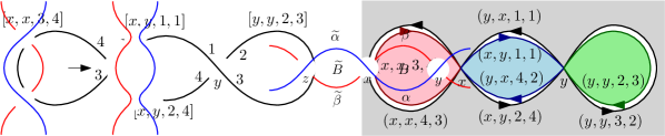
Figure 3: Left: Representation of the diagram in the figure is given by setting $V(D)=\{x,y\}$, and adding edges $[x,x,3,4]$, $[x,y,1,1]$, $[y,y,2,3]$ and $[x,y,2,4]$. Right: Each edge corresponds to a pair of edges, in which case, the directed edges determine faces. In our case, we have bounded faces $\{(x,x,3,4)\}$, $\{(x,y,1,1),(y,x,4,2)\}$, $\{(y,y,2,3)\}$ and unbounded face $\{(x,x,4,3),(y,x,1,1),(y,y,3,2),(x,y,2,4)\}$.

We remark that we consider the edges unoriented, that is, $[v_{1},v_{2},n_{1},n_{2}]=[v_{2},v_{1},n_{2},n_{1}]$. However, for purpose of representing faces, it is convenient to follow the idea of doubly-connected edge list (see [dBCvKO08]) so that each edge $[v_{1},v_{2},n_{1},n_{2}]$ is represented as a pair of oriented edges $(v_{1},v_{2},n_{1},n_{2})$ and $(v_{2},v_{1},n_{2},n_{1})$ where $(v_{1},v_{2},n_{1},n_{2})$ stands for the directed edge leaving $v_{1}$ via strand marked $n_{1}$ and entering $v_{2}$ via strand $n_{2}$. Each directed edge uniquely determines a face on the ‘right hand side’ and if two oriented edges $(v_{1},v_{2},n_{1},n_{2})$ and $(v_{3},v_{4},n_{3},n_{4})$ satisfy $v_{2}=v_{3}$ and $n_{2}=n_{3}+1\pmod{4}$, then they determine the same face; see Figure 4. If we declare two such oriented edges as equivalent, then faces of $D$ can be represented as the classes of the (inclusion-wise) smallest equivalence containing such pairs of equivalent oriented edges; see Figure 3, right. In order to complete our combinatorial description of a diagram, it remains to mark one face as the outer face—the unique unbounded face. (Of course, not every choice of $V(D)$ and $4$-tuples $[v_{1},v_{2},n_{1},n_{2}]$ as above yields a valid representation of a diagram. In our considerations, we will assume that we really have a valid representation.)

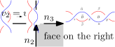
Figure 4: Directed edges pointing to the same face on the right.

We remark that if we have a diagram $D$ with $n$ crossings, then this way we can reach an encoding of $D$ of size $O(n\log n)$ if we interpret crossings as integers in binary. For purposes of the implementation of the algorithm, we always assume that we have an encoding of $D$ of such size. However, for purposes of the analysis of the algorithm, $V(D)$ will be just some abstract set.

3 Reidemeister moves

3.1 Combinatorial description of Reidemeister moves

Given a diagram represented combinatorially as explained earlier, we want to provide a combinatorial description of all feasible Reidemeister moves in $D$. When doing so, we will have the following aims.

• We want to describe each move with as less combinatorial data as possible that is required to determine a given move uniquely. For example, it is not hard to see that a $\rm{II}^{-}$ move in a diagram $D$ is uniquely determined by the two crossings removed by the move. Thus it makes sense to identify $\rm{II}^{-}$ moves with pairs of crossings of $D$. The cost of this approach is that not every pair of crossings in a given diagram yields a feasible $\rm{II}^{-}$ move. Thus we have to distinguish which pairs do.

• The previous approach allows us to say, in some cases, that two moves in different diagrams are (combinatorially) the same. For example, if we have diagrams $D$ and $D^{\prime}$ both of them containing crossings $x$ and $y$ and in both diagrams there is a feasible $\rm{II}^{-}$ move removing $x$ and $y$. Then we can regard this move as the same move in both cases. This will be useful in stating various rearrangement lemmas on the ordering of the moves in a sequence of moves untangling a given diagram.

• We want to be able to enumerate all possible Reidemeister moves in a given diagram in polynomial time. This can be regarded as obvious but we want to include the details for completeness. Thus, for this aim, we can use the combinatorial description in the first item above and check feasibility in each case.

• For running and analysing our algorithm, it will be also useful if a feasible move $m$ in a diagram $D$ uniquely determines the combinatorial description of the resulting diagram $D(m)$ after performing the move.

Our description of the moves will in particular yield a proof of the following lemma.

Lemma 4.

Let $D$ be a diagram of a knot with $n$ crossings (and with encoding of size $O(n\log n)$).

1. There are $O(n^{2})$ feasible Reidemeister moves and all of them can be enumerated in time $O(n^{2}\log n)$.

2. Given a feasible move $m$ in $D$, the diagram $D(m)$ can be constructed in time $O(n\log n)$.

We prove the lemma simultaneously with our description of the moves.

We start with $\rm{I}^{-}$, $\rm{II}^{-}$ and $\rm{III}$ moves:

$\rm{I}^{-}$, $\rm{II}^{-}$ and $\rm{III}$ moves: Definitions.

By a simple case analysis, each feasible Reidemeister $\rm{I}^{-}$, $\rm{II}^{-}$ or $\rm{III}$ move $m$ in $D$ is uniquely determined by the set of crossings $X$ in $D$ affected by the move. In the case of $\rm{I}^{-}$ move there is seemingly an exceptional case of a diagram with a single crossing and two loops attached to the crossing; see Figure 5. However, the resulting diagram after performing the $\rm{I}^{-}$ move is $U$ independently of the choice of the loop which is removed. Thus we do not really distinguish these two cases. Therefore, we can define a $\rm{I}^{-}$ move in $D$ as a $1$-element subset of $V(D)$, a $\rm{II}^{-}$ move as a $2$-element subset of $V(D)$, and a $\rm{III}$ move as a $3$-element subset of $V(D)$. In this terminology, not every $\rm{I}^{-}$, $\rm{II}^{-}$ or $\rm{III}$ move yields feasible Reidemeister move, thus we always add the adjective feasible if it indeed yields.

We find it often convenient to emphasize the type of the move in the notation (if we know it), thus we also write $\{x\}_{\rm{I}^{-}}$ instead of $\{x\}$ for a $\rm{I}^{-}$ move removing $\{x\}$, and similarly we use $\{x,y\}_{\rm{II}^{-}}$ and $\{x,y,z\}_{\rm{III}}$.

Figure 5: The resulting diagram after applying $\rm{I}^{-}$ move does not depend on the choice of the loop which is removed.

$\rm{I}^{-}$, $\rm{II}^{-}$ and $\rm{III}$ moves: Checking feasibility.

For checking whether a given $\rm{I}^{-}$, $\rm{II}^{-}$, or a $\rm{III}$ move is feasible in a given diagram, we can use the following approach.

In case of a $\rm{I}^{-}$ move $\{x\}_{\rm{I}^{-}}$, it is sufficient to check whether $D$ contains an $[x,x,n_{1},n_{2}]$ edge where $n_{1},n_{2}\in\{1,2,3,4\}$ such that one of the outer edges $(x,x,n_{1},n_{2})$ or $(x,x,n_{2},n_{1})$ forms a face different from the outer face of $D$. Therefore, if we want to find all feasible $\rm{I}^{-}$ moves, then it is sufficient to find all faces formed by a single directed edge and check whether they are distinct from the outer face. This can be done in time $O(n\log n)$ where $n$ is the number of crossings due to encoding the crossings as integers in binary.

In case of a $\rm{II}^{-}$ move $\{x,y\}_{\rm{II}^{-}}$, we need a face, distinct from the outer face, formed by two directed edges $(x,y,n_{1},n_{2})$ and $(y,x,n_{3},n_{4})$. In addition we need that one of the edges $[x,y,n_{1},n_{2}]$ and $[y,x,n_{3},n_{4}]$ enters both $x$ and $y$ as overpass and the other one as underpass. This can be determined from $n_{1}$, $n_{2}$, $n_{3}$ and $n_{4}$. Therefore, if we want to enumerate all feasible $\rm{II}^{-}$ moves, we can do it in time $O(n\log n)$ where $n$ is the number of crossings due to encoding the crossings as integers in binary.

In case of a $\rm{III}$ move $\{x,y,z\}_{\rm{III}}$, we need a face, distinct from the outer face, formed by three directed edges $(x,y,n_{1},n_{2})$, $(y,z,n_{3},n_{4})$, $(z,x,n_{5},n_{6})$ up to a permutation of $\{x,y,z\}$. We also need that one of the edges $[x,y,n_{1},n_{2}]$, $[y,z,n_{3},n_{4}]$, or $[z,x,n_{5},n_{6}]$ enters both its endpoints as overpass, the second one enters one endpoint as overpass and the other one as underpass, and the third one enters both its endpoints as underpass. This can be determined by providing a finite list of allowed options for $(n_{1},n_{2},n_{3},n_{4},n_{5},n_{6})$. Altogether, we can again enumerate all feasible $\rm{III}$ moves in time $O(n\log n)$ where $n$ is the number of crossings due to encoding the crossings as integers in binary.

$\rm{I}^{-}$, $\rm{II}^{-}$ and $\rm{III}$ moves: Construction of $D(m)$.

Now, we briefly describe how to get $D(m)$ from the knowledge of $D$ and $m$.

Let us start with a $\rm{I}^{-}$ move as in Figure 6. Assume that it removes a crossing $x$ and that the strands around $x$ are numbered as in the figure. Assume also that the loose ends of the arc affected by the move head to crossings $x^{\prime}$ and $x^{\prime\prime}$ via strands numbered $n^{\prime}$ and $n^{\prime\prime}$. Then we get $D(m)$ from $D$ by removing $x$ and the edges $[x,x,n_{2},n_{3}]$, $[x,x^{\prime},n_{4},n^{\prime}]$, and $[x,x^{\prime\prime},n_{1},n^{\prime\prime}]$ while adding an edge $[x^{\prime},x^{\prime\prime},n^{\prime},n^{\prime\prime}]$. (There is a single exception, though: If $x=x^{\prime}=x^{\prime\prime}$, then $D(m)=U$ is the diagram without crossings.) We also need to update the list of faces, but this is straightforward. In the case in the figure, for the face of $D$ containing directed edges $(x^{\prime\prime},x,n^{\prime\prime},n_{1})$ and $(x,x^{\prime},n_{4},n^{\prime})$ these two edges get replaced with the directed edge $(x^{\prime\prime},x^{\prime},n^{\prime\prime},n^{\prime})$. Similarly, for the face containing $(x^{\prime},x,n^{\prime},n_{4}),(x,x,n_{3},n_{2}),(x,x^{\prime\prime},n_{1},n^{\prime\prime})$ these edges get replaced with $(x^{\prime},x^{\prime\prime},n^{\prime},n^{\prime\prime})$. Altogether, we perform a constant number of operations. However, as we are removing some crossings, we may want to relabel the crossings, if we want to reach a representation of $D(m)$ of size $O(\widehat{n}\log\widehat{n})$ where $\widehat{n}$ is the number of crossings of $D(m)$. Doing so naively (which is fully sufficient for our purposes), we may need time $O(n\log n)$ for this. But we do this relabelling only for the purpose of implementing the algorithm. For the analysis of the algorithm, we keep the names the same.

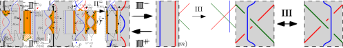
Figure 6: $D(m)$ coming from $D$ after a $\rm{I}^{-}$ move. Here we cover both cases whether the strands at $n_{1}$ and $n_{3}$ are underpasses or overpasses, thus we didn’t make an explicit choice in the figure.

Moves of types $\rm{II}^{-}$ or $\rm{III}$ can be treated similarly, and we omit most of the details, because we believe that the general approach can be understood from the $\rm{I}^{-}$ example, while it is a bit tedious to list all possible cases. Thus we only point out important differences. For a $\rm{II}^{-}$ move $m=\{x,y\}_{\rm{II}^{-}}$ there are a few more exceptional cases how to rebuild the diagram depending on whether there are loops at $x$ or at $y$. (Note that there cannot be three edges connecting $x$ and $y$ if we have a diagram of a knot.) For a $\rm{III}$ move $m=\{x,y,z\}_{\rm{III}}$ there are again more exceptional cases, depending whether there loops at $x$, $y$, $z$ or additional edges connecting two of the points among $x$, $y$, $z$. In addition, we want to keep the names of the crossings during the move. Consider the move on Figure 7; here for simplicity of the figure, we label the strands only around $z$ on the left figure and around $x$ on the right figure. We shift the labels of the crossings as indicated in the figure. For example, $x$ is an intersection of arcs $\alpha$ and $\beta$ in the left figure. These two arcs are shifted to $\alpha^{\prime}$ and $\beta^{\prime}$ in the right figure and we label the intersection of $\alpha^{\prime}$ and $\beta^{\prime}$ again by $x$. Regarding the edges when coming from $D$ to $D(m)$, for example the edge $[z,z^{\prime\prime},n_{1},n_{z}^{\prime\prime}]$ is removed while it is replaced with the edge $[x,z^{\prime\prime},1,n_{z}^{\prime\prime}]$.

Figure 7: Crossings before and after a $3$-move.

$\rm{I}^{-}$, $\rm{II}^{-}$ and $\rm{III}$ moves: Circle.

We will also need the following notion: for a feasible Reidemeister $\rm{I}^{-}$, $\rm{II}^{-}$, or $\rm{III}$ move $m$ affecting the set of crossings $X$ on a diagram with at least two crossings, we will also denote by $c(m)\subseteq{\mathbb{R}}^{2}$ the unique circle formed by images of edges in $D$ which contains the crossings of $X$ but no other crossings; see Figure 8. (Here we regard a diagram and edge as topological notions according to our earlier definitions). We will refer to $c(m)$ as to the circle of $m$.

Figure 8: The circle $c(m)$ of a feasible $\rm{I}^{-}$, $\rm{II}^{-}$, or $\rm{III}$ move $m$. For emphasizing $c(m)$ the overpasses are not depicted.

$\rm{I}^{+}$ moves: Definitions.

We define a $\rm{I}^{+}$ move as a pair $(\overrightarrow{\varepsilon},\sigma)$, where $\overrightarrow{\varepsilon}$ is a directed edge of $D$ and $\sigma\in\{+,-\}$. Here $\overrightarrow{\varepsilon}$ determines the undirected edge $\varepsilon$ on which the move is performed as well as the side on which the loop is introduced. For being consistent with our definition of faces, we require that the loop is introduced on the right hand-side of $\overrightarrow{\varepsilon}$. The sign determines whether the crossing is positive or negative with respect to the orientation of $\overrightarrow{\varepsilon}$; see Figure 9. In an exceptional case $D=U$, $\overrightarrow{\varepsilon}$ represents $U$ with positive or negative orientation.

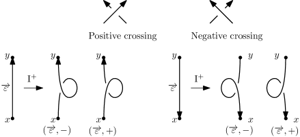
Figure 9: Positive and negative crossings and four options for $\rm{I}^{+}$ affecting a given edge.

$\rm{II}^{+}$ moves: Definitions.

Any feasible Reidemeister ${\rm{II}^{+}}$ move can be performed in the following way. We pick two points $a$, $b$ on $D$ different from crossings. We connect them with a standard topological arc $\zeta$ inside one of the faces of $D$ (except of the endpoints $a$, $b$ which do not belong to the face). We pull a finger from $a$ towards $b$ along $\zeta$, thereby performing the ${\rm{II}^{+}}$ move; see Figure 10. We may assume that the finger overpasses $b$ because an underpass could be obtained, up to isotopy, by pulling a finger from $b$ to $a$ along $\zeta$.

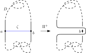
Figure 10: A ${\rm{II}^{+}}$ move along $\zeta$.

This means that any feasible ${\rm{II}^{+}}$ move is uniquely determined by the following data.

• A pair of directed edges $(\overrightarrow{\varepsilon},\overrightarrow{\varphi})$ on which the move is performed, subject to the condition that $\overrightarrow{\varepsilon}$ and $\overrightarrow{\varphi}$ belong to the same face $f$. Comparing with the description above, $a$ would belong to $\overrightarrow{\varepsilon}$, $b$ would belong to $\overrightarrow{\varphi}$, and $\zeta$ would belong to the face containing $\overrightarrow{\varepsilon}$ and $\overrightarrow{\varphi}$. (Here we mean the containment in the combinatorial sense where a face is a collection of directed edges.) We remark that we explicitly allow $\overrightarrow{\varepsilon}=\overrightarrow{\varphi}$ (this corresponds to the case when $a$ and $b$ belong to the same edge).

• A winding $w\in\{+,-\}$. The winding is relevant only if $f$ is the unbounded face. For fixed $a$ and $b$, the winding determines $\zeta$ up to isotopy. Indeed, first consider the case that $f$ is bounded, then $f$ is homeomorphic to an open disk (because $D$ is a diagram of a knot) and then $\zeta$ is unique up to isotopy. If $f$ is unbounded, then $f$ is homeomorphic to an open annulus. This is easy to see in one point compatification of ${\mathbb{R}}^{2}$ by adding a point $\infty$ thereby obtaining the sphere $S^{2}$. Then $f\cup\{\infty\}$ is a (necessarily bounded) face in $S^{2}$ therefore an open disk. Consequently, $f$ is an open disk minus a point that is an open annulus. Then we have two options, either $\zeta$ passes from $a$ to $b$ in positive direction or negative direction; see Figure 11. Then we set $w=+$ in the former case and $w=-$ in the latter case.

  

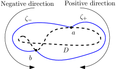
  Figure 11: If $\zeta$ belongs to the unbounded face, there are two possible isotopy classes for $\zeta$.

• An order (of $a$ and $b$) denoted $o\in\{1,2\}$. The order is relevant only if $\overrightarrow{\varepsilon}=\overrightarrow{\varphi}$. Indeed, if $\overrightarrow{\varepsilon}\neq\varphi$, then any shift of $a$ along $\overrightarrow{\varepsilon}$ or any shift of $b$ along $\overrightarrow{\varphi}$ yields an isotopic $\rm{II}^{+}$, therefore the data above uniquely determine the move. (Note that if $\overrightarrow{\varepsilon}\neq\overrightarrow{\varphi}$, then also the undirected edges determined by $\overrightarrow{\varepsilon}$ and $\overrightarrow{\varphi}$ are distinct because $\overrightarrow{\varepsilon}$ and $\overrightarrow{\varphi}$ belong to the same face $f$.) If $\overrightarrow{\varepsilon}=\overrightarrow{\varphi}$, it remains to distinguish whether $a$ precedes $b$ along $\overrightarrow{\varepsilon}$ or whether $b$ precedes $a$. In the former case we set $o=1$, in the latter case, we set $o=2$.

Thus we define a ${\rm{II}^{+}}$ move as quadruple $(\overrightarrow{\varepsilon},\overrightarrow{\varphi},w,o)$ as above. If, for example, $w$ is irrelevant for given $\overrightarrow{\varepsilon}$, $\overrightarrow{\varphi}$ and $o$, then $(\overrightarrow{\varepsilon},\overrightarrow{\varphi},+,o)$ and $(\overrightarrow{\varepsilon},\overrightarrow{\varphi},-,o)$ yield the same move and we regard them as the same combinatorial object. The most complex case when $\zeta$ is in the unbounded face and $\overrightarrow{\varepsilon}=\overrightarrow{\varphi}$ is depicted at Figure 12.

Figure 12: Four possible outputs of an ${\rm{II}^{+}}$ move depending on $w$ and $o$.

In an exceptional case when $D=U$, $\overrightarrow{\varepsilon}$ and $\overrightarrow{\varphi}$ represent $U$ with a positive or negative orientation. This orientation has to be the same for $\overrightarrow{\varepsilon}$ and $\overrightarrow{\varphi}$.

$\rm{I}^{+}$ moves and $\rm{II}^{+}$ moves: Checking feasibility.

There is nothing to do regarding checking feasibility for $\rm{I}^{+}$ and $\rm{II}^{+}$ moves. Every $\rm{I}^{+}$ move $(\overrightarrow{\varepsilon},\sigma)$ is feasible. Similarly, every ${\rm{II}^{+}}$ move $(\overrightarrow{\varepsilon},\overrightarrow{\varphi},w,o)$ is feasible subject to the condition $\overrightarrow{\varepsilon}$ and $\overrightarrow{\varphi}$ belong to a same face. Thus the number of feasible $\rm{I}^{+}$ moves or $\rm{II}^{+}$ moves is at most quadratic in $n$, and they can be enumerated in time $O(n^{2}\log n)$ due to encoding the labels of the crossings in binary.

$\rm{I}^{+}$ moves and $\rm{II}^{+}$ moves: Construction of $D(m)$.

For a construction of $D(m)$ for a $\rm{I}^{+}$ move $m$, we can invert the process explained for a $\rm{I}^{-}$ move; see again Figure 6 (of course, in this case, we need to set $n_{1},n_{2},n_{3},n_{4}$ as concrete numbers depending on the sign of $m$). We also need to treat the case $D=U$ separately. It is similarly straightforward to treat $\rm{II}^{+}$ moves while $D=U$ is again an exceptional case.

The only missing information, if we want to get $D(m)$ uniquely is to add the names of the newly introduced crossings. Here, our convention depends on the purpose. If we want to construct $D(m)$ for the algorithm, then we pick the label of the new crossing as the first available integer in binary so that we get $D(m)$ of correct size. On the other hand for the purpose of analysis of the algorithm when we consider $V(D)$ as an abstract set, we assume that the newly introduced crossings have fresh new labels that haven’t been used previously (in case that $D(m)$ is an intermediate step of some sequence of Reidemeister moves on some diagram).

This also finishes the proof of Lemma 4 by checking how much which moves contribute to each item of the lemma.

A piece of notation for diagrams.

Here we extend our notation $D(m)$ to several consecutive moves. We inductively define the notation $D(m_{1},\dots,m_{k-1},m_{k}):=D(m_{1},\dots,m_{k-1})(m_{k})$ provided that $m_{k}$ is a feasible Reidemeister move in $D(m_{1},\dots,m_{k-1})$. We also say that a sequence $(m_{1},\dots,m_{k})$ is a feasible sequence of Reidemeister moves for $D$ if $m_{i}$ is a feasible Redemeister move in $D(m_{1},\dots,m_{i-1})$ for every $i\in[k]$.

3.2 Special and greedy moves revisited

Let $X$ be a set of crossings in diagram $D$. We say that a move $m$ avoids $X$ if $m$ is

• a $\rm{I}^{-}$ move removing a crossing $x\not\in X$, or

• a $\rm{II}^{-}$ move removing crossings $x,y\not\in X$, or

• a $\rm{III}$ move affecting crossings $x,y,z\not\in X$, or

• a $\rm{I}^{+}$ move performed on an edge $\varepsilon$ such that no endpoint of $\varepsilon$ belongs to $X$, or

• a ${\rm{II}^{+}}$ move performed on edges $\overrightarrow{\varepsilon}$, $\overrightarrow{\varphi}$ (possibly $\overrightarrow{\varepsilon}=\overrightarrow{\varphi}$) such that no endpoint of any of these two edges belongs to $X$.

Let us recall from the introduction that given a set $S$ of crossings in a diagram $D$, a feasible Reidemeister move $m$ is greedy (with respect to $S$) if it is a $\rm{II}^{-}$ move avoiding $S$. The definition of a special move from the introduction can be equivalently reformulated so that $m$ is special (with respect to $S$) if it avoids crossings not in $S$, that is, the set $V(D)\setminus S$.

Obviously, it may happen that some feasible move in $D$ is neither greedy nor special with respect to $S$. Because of our algorithm SpecialGreedy, we will be interested in sequences of moves on $D$ such that each move is either greedy or special. However, the set $S$ may vary while performing the special moves, thus we need to be a bit careful with the definitions.

Given a move $m$ in $D$, we denote by $X(m)$ the following set of crossings in $D(m)$.

• If $m$ is a $\rm{III}$ move, then $X(m)=\emptyset$.

• If $m$ is a $\rm{II}^{-}$ move or a $\rm{I}^{-}$ move, then $X(m)$ is the set of crossings removed by $m$.

• If $m$ is a $\rm{I}^{+}$ or a ${\rm{II}^{+}}$ move, then $X(m)$ is the set of crossings introduced by $m$.

Let $\triangle$ denote the symmetric difference of two sets. We get the following observation.

Observation 5.

Let $m$ be a special or greedy move in a diagram $D$ with respect to a set $S$. Let $S(m)$ be the set defined in the introduction when describing the SpecialGreedy algorithm. Then

• $S(m)=S$ if $m$ is greedy; while

• $S(m)=S\triangle X(m)$ if $m$ is special.

Proof.

The first item is exactly the definition of $S(m)$ for a greedy move. For the second item, when compared with the definition in the introduction, we have defined $X(m)$ as $S\triangle S(m)$ from which the observation follows. ∎

In the remainder of the paper, we plan to use 5 as an equivalent definition of $S(m)$. The advantage of this reformulation is that $X(m)$ does not depend on $S$.

Feasible moves for pairs.

Now we aim to extend our definition of a feasible sequence $(m_{1},\dots,m_{\ell})$ of Reidemeister moves in a diagram $D$ to a pair $(D,S)$ where $S$ is a set of crossing of $D$ so that we allow only special or greedy moves. For this, we say that $m$ is a feasible move for a pair $(D,S)$ if it is a move in $D$ special or greedy with respect to $S$. If $m$ is feasible for $(D,S)$, then we also use the notation $(D,S)(m)$ for the resulting pair after performing the move, that is, $(D,S)(m):=(D(m),S(m))$. Now, we inductively define the notation $(D,S)(m_{1},\dots,m_{\ell-1},m_{\ell}):=(D,S)(m_{1},\dots,m_{\ell-1})(m_{\ell})$ provided that $m_{\ell}$ is a feasible Reidemeister move in $(D,S)(m_{1},\dots,m_{\ell-1})$. We also say that a sequence $(m_{1},\dots,m_{\ell})$ is a feasible sequence of Reidemeister moves for $(D,S)$ if $m_{i}$ is a feasible move in $(D,S)(m_{1},\dots,m_{i-1})$ for every $i\in[\ell]$. It also may be convenient to write $(D,S)(m_{1},\dots,m_{\ell-1},m_{\ell})$ directly as a pair $(D^{\prime},S^{\prime})$. In this case, we get $D^{\prime}=D(m_{1},\dots,m_{\ell})$ which follows immediately from the earlier definition of $D(m_{1},\dots,m_{\ell})$ and we define $S(m_{1},\dots,m_{\ell})$ as $S^{\prime}$ above. From the definition above, we also get $S(m_{1},\dots,m_{\ell})=S(m_{1},\dots,m_{\ell-1})(m_{\ell})$. However, we have to be a bit careful about how to interpret this formula: $m_{\ell}$ is regarded here as a move in $D(m_{1},\dots,m_{\ell-1})$ special or greedy with respect to $S(m_{1},\dots,m_{\ell-1})$ although $D(m_{1},\dots,m_{\ell-1})$ does not really appear in the notation. We get the following extension of 5.

Lemma 6.

Let $(m_{1},\dots,m_{\ell})$ be a feasible sequence for a pair $(D,S)$ where $D$ is a diagram and $S$ is a set of crossings. Then

$$S(m_{1},\dots,m_{\ell})=S\triangle X(m_{i_{1}})\triangle\cdots\triangle X(m_{i_{s}})$$

where $(i_{1},\dots,i_{s})$ is the subsequence of $(1,\dots,\ell)$ consisting of exactly the indices $i_{j}$ such that $m_{i_{j}}$ is special in $D(m_{1},\dots,m_{i_{j}-1})$ with respect to $S(m_{1},\dots,m_{i_{j}-1})$.

Proof.

The proof follows by induction in $\ell$. If $\ell=1$, then it directly follows from 5.

If $\ell>1$, let $(i_{1},\dots,i_{s})$ be the subsequence of $(1,\dots,\ell-1)$ consisting of exactly the indices $i_{j}$ such that $m_{i_{j}}$ is special in $D(m_{1},\dots,m_{i_{j}-1})$ with respect to $S(m_{1},\dots,m_{i_{j}-1})$. Let us distinguish whether $m_{\ell}$ is greedy or special (in $D(m_{1},\dots,m_{\ell-1})$ with respect to $S(m_{1},\dots,m_{\ell-1})$).

If $m_{\ell}$ is greedy, then by induction and by 5 applied to $m_{\ell}$ we get

$$S(m_{1},\dots,m_{\ell})=S(m_{1},\dots,m_{\ell-1})(m_{\ell})=(S\triangle X(m_{i_{1}})\triangle\cdots\triangle X(m_{i_{s}}))(m_{\ell})=S\triangle X(m_{i_{1}})\triangle\cdots\triangle X(m_{i_{s}})$$

as required.

Similarly, if $m_{\ell}$ is special, we get

$$S(m_{1},\dots,m_{\ell})=(S\triangle X(m_{i_{1}})\triangle\cdots\triangle X(m_{i_{s}}))(m_{\ell})=S\triangle X(m_{i_{1}})\triangle\cdots\triangle X(m_{i_{s}})\triangle X(m_{\ell})$$

as required. ∎

As a consequence, we also get the following description of $S(m_{1},\dots,m_{\ell})$.

Lemma 7.

Let $D$ be a diagram of a knot, $S$ be a set of crossings in $D$ and $(m_{1},\dots,m_{\ell})$ be a feasible sequence for the pair $(D,S)$. Then $S(m_{1},\dots,m_{\ell})$ contains exactly the crossings in $D(m_{1},\dots,m_{\ell})$ which either already belong to $S$ or do not belong to $D$.

Proof.

Let $x$ be a crossing in $D(m_{1},\dots,m_{\ell})$. If $x$ does not belong to any of $X(m_{i_{1}}),\dots,X(m_{i_{s}})$ where $(i_{1},\dots,i_{s})$ is a sequence as in Lemma 6, then $x$ necessarily belongs to $D$ and in addition it belongs to $S$ if and only if it belongs to $S(m_{1},\dots,m_{\ell})$ by Lemma 6, which is exactly what we need.

If $x$ belongs to some $X(m_{i_{j}})$, then $m_{i_{j}}$ is necessarily a $\rm{I}^{+}$ or a ${\rm{II}^{+}}$ move, otherwise $x$ would be removed by $m_{i_{j}}$ and according to our conventions it cannot be reintroduced later on with the same label (but we know that $x$ belongs to $D(m_{1},\dots,m_{\ell})$). We also get that in this case $m_{i_{j}}$ is unique as $x$ cannot be added to the diagram twice. Thus $x$ does not belong to $D$ while it belongs to $S(m_{1},\dots,m_{\ell})$ due to Lemma 6 which is what we need. ∎

The following lemma shows that if the diagram can be untangled with defect $d$, then there exists a choice of $S$ at step 0 of the algorithm SpecialGreedy$(D,k)$ that will allow the algorithm to find an untangling sequence.

Lemma 8.

Let $D$ be a diagram of a knot and let $(m_{1},\dots,m_{\ell})$ be a feasible sequence of Reidemeister moves in $D$. Then there is a set of crossings $S$ in $D$ such that $(m_{1},\dots,m_{\ell})$ is feasible for $(D,S)$.

In addition, if this sequence induces an untangling with defect at most $k$, then $|S|\leq 3k$.

Proof.

First, we put a crossing $x$ of $D$ into an auxiliary set $S^{\prime}$ in the following cases:

• If $x$ is removed by a $\rm{I}^{-}$ move in the sequence.

• If $x$ is affected by some $\rm{III}$ move in the sequence.

• If there is a $\rm{I}^{+}$ move or a ${\rm{II}^{+}}$ move performed on an edge with endpoint $x$.

Then we define $S^{\prime\prime}$ as a set of crossings $x$ in $V(D)\setminus S^{\prime}$ such that there is $y\in S^{\prime}$ such that $x$ and $y$ are simultaneously removed by a $\rm{II}^{-}$ move in the sequence $(m_{1},\dots,m_{\ell})$ and $S^{\prime\prime\prime}$ as a set of crossings $x$ in $V(D)\setminus S^{\prime}$ such that $x$ is removed by a $\rm{II}^{-}$ move in the sequence $(m_{1},\dots,m_{\ell})$ simultaneously with some crossing $y$ not belonging to $V(D)$ (that is, with $y$ which is introduced by some $\rm{I}^{+}$ or ${\rm{II}^{+}}$ move before applying the move removing $x$ and $y$). See Figure 13 for an example how may $S^{\prime}$, $S^{\prime\prime}$ and $S^{\prime\prime\prime}$ look like. We set $S:=S^{\prime}\cup S^{\prime\prime}\cup S^{\prime\prime\prime}$ and we want to check that $(m_{1},\dots,m_{\ell})$ is feasible with respect to $S$.

Figure 13: Consider a slightly artificial untangling of the diagram $D$ in the top left corner, given by the sequence $(m_{1},\dots,m_{7})$. Then $x_{5}$, $x_{6}$ and $x_{7}$ belong to $S^{\prime}$ because they are endpoints of edges on which the ${\rm{II}^{+}}$ move $m_{1}$ is performed (another reason why $x_{6}$ and $x_{7}$ are in $S^{\prime}$ is that they are removed by $\rm{I}^{-}$ moves $m_{6}$ and $m_{7}$). Consequently $x_{4}\in S^{\prime\prime}$ because it is removed simultaneously with $x_{5}\in S^{\prime}$ by a $\rm{II}^{-}$ move $m_{2}$. We also get $x_{3}\in S^{\prime\prime\prime}$ because it is removed simultaneously with $y_{1}\not\in V(D)$ by a $\rm{II}^{-}$ move $m_{3}$. The move $m_{4}$ is the only greedy move in this sequence, all other moves are special.

In other words, we want to check that for every $i\in[\ell]$, the move $m_{i}$ is either special or greedy in $D(m_{1},\dots,m_{i-1})$ with respect to $S(m_{1},\dots,m_{i-1})$. For simplicity of notation, let $D_{i-1}:=D(m_{1},\dots,m_{i-1})$ and $S_{i-1}:=S(m_{1},\dots,m_{i-1})$. We will distinguish several cases according to the type of $m_{i}$.

If $m_{i}$ is a $\rm{I}^{-}$ move removing a crossing $x$ in $D_{i-1}$ then either $x$ belongs to $D$ or it has been introduced by some previous $\rm{I}^{+}$ or ${\rm{II}^{+}}$ move (see Lemma 7). If $x$ belongs to $D$ then it belongs to $S^{\prime}$ by the first condition of the definition of $S^{\prime}$, consequently $x$ belongs to $S$ and $S_{i-1}$ as well by the definition of $S_{i-1}$. If $x$ has been introduced by some previous $\rm{I}^{+}$ or ${\rm{II}^{+}}$ move, then it belongs to $S_{i-1}$ by the definition of $S_{i-1}$ (newly introduced vertex is always added). In particular $m_{i}$ is special with respect to $S$.

If $m_{i}$ is a $\rm{III}$ move then by analogous reasoning, using the second condition in the definition of $S^{\prime}$, we deduce that every crossing affected by $m_{i}$ belongs to $S_{i-1}$. Therefore $m_{i}$ is special as well.

If $m_{i}$ is a $\rm{I}^{+}$ or a ${\rm{II}^{+}}$ move, let $E$ be the set of endpoints in $D_{i-1}$ of the edges on which $m_{i}$ is performed. Again by similar reasoning, using the third condition in the definition of $S^{\prime}$, we get that all crossings in $E$ belong to $S_{i-1}$. Therefore $m_{i}$ is special as well.

The last case is to consider when $m_{i}$ is a $\rm{II}^{-}$ move. Let us say that $m_{i}$ removes crossings $x$ and $y$. If any of these crossings does not belong to $D$, then it belongs to $S_{i-1}$ by Lemma 7 and the other crossing either does not belong to $D$ as well which implies that it belongs to $S_{i-1}$, or it belongs to $D$ which implies that it belongs to $S^{\prime}$ or $S^{\prime\prime\prime}$ by the definition of $S^{\prime\prime\prime}$. Altogether the other crossing belongs to $S_{i-1}$ in each case and $m_{i}$ is special. Thus we may assume that both $x$ and $y$ belong to $D$. If one of them belongs to $S^{\prime}$ then the other one belongs to $S^{\prime}$ or $S^{\prime\prime}$ and consequently $m_{i}$ is special. If none of them belongs to $S^{\prime}$ then none of them belongs to $S^{\prime\prime}\cup S^{\prime\prime\prime}$ by the definition of $S^{\prime\prime}$ and $S^{\prime\prime\prime}$, thus none of them belongs to $S$. Therefore $m_{i}$ is greedy in this case.

It remains to bound the size of $S$. Let $c^{+}(m_{i})$ be the number of newly created crossings by a move $m_{i}$ and let $c^{\prime}(m_{i})$ be the number of crossings inserted into $S^{\prime}$ because of $m_{i}$. Explicitly, if $m_{i}$ is a $\rm{I}^{-}$ move, then we count the crossing removed by $m_{i}$ (if present in $D$) that is $c^{\prime}(m_{i})\leq 1$; if $m_{i}$ is a $\rm{II}^{-}$ move there is no such crossing, thus $c^{\prime}(m_{i})=0$; if $m_{i}$ is a $\rm{III}$ move then there are at most three such crossings affected by $m_{i}$, thus $c^{\prime}(m_{i})\leq 3$; if $m_{i}$ is a $\rm{I}^{+}$ move then there are at most two such crossings as the endpoints of the edge on which is $m_{i}$ performed, thus $c^{\prime}(m_{i})\leq 2$; and if $m_{i}$ is a ${\rm{II}^{+}}$ move then there are at most four such endpoints thus $c^{\prime}(m_{i})\leq 4$. Altogether, by considering the values $c^{+}(m_{i})$, we get that $c^{+}(m_{i})+c^{\prime}(m_{i})\leq\frac{3}{2}w(m_{i})$ where $w(m_{i})$ is the weight defined before  Lemma 3.

On the other hand, we get the following inequalities:

$$|S^{\prime}|\leq\sum_{i=1}^{\ell}c^{\prime}(m_{i})$$

by the definition of $c^{\prime}(m_{i})$;

$$|S^{\prime\prime}|\leq|S^{\prime}|\leq\sum_{i=1}^{\ell}c^{\prime}(m_{i})$$

by the definition of $S^{\prime\prime}$ and the previous inequality; and

$$|S^{\prime\prime\prime}|\leq\sum_{i=1}^{\ell}c^{+}(m_{i})$$

by the definition of $c^{+}(m_{i})$ and $S^{\prime\prime\prime}$. Altogether, we get

$$|S|\leq|S^{\prime}|+|S^{\prime\prime}|+|S^{\prime\prime\prime}|\leq\sum_{i=1}^{\ell}2(c^{\prime}(m_{i})+c^{+}(m_{i}))\leq\sum_{i=1}^{\ell}3w(m_{i})\leq 3k$$

where the last inequality uses Lemma 3. ∎

We finish this section by stating the following theorem that is the key ingredient for the proof of correctness of our SpecialGreedy$(D,k)$ algorithm. Namely, it shows that we cannot make wrong choice in Step 2 of the algorithm.

Theorem 9.

Let $D$ be a diagram of a knot and $S$ be a set of crossings in $D$. Let $(m_{1},\dots,m_{\ell})$ be a feasible sequence of Reidemeister moves for $(D,S)$, inducing an untangling of $D$ with defect $k$. Assume that there is a greedy move $\widetilde{m}$ in $D$ with respect to $S$. Then there is a feasible sequence of Reidemeister moves for $(D,S)$ starting with $\widetilde{m}$ and inducing an untangling of $D$ with defect $k$.

The proof of this theorem is given at the end of Section 5.

4 W[P]-membership modulo Theorem 9.

Assuming Theorem 9 we have collected enough tools to show that SpecialGreedy$(D,k)$ is a W[P]-algorithm which provides a correct answer to Unknotting via defect. Because this part is technically easier and because some auxiliary lemmas are more fresh now, we show this before proving Theorem 9. For the reader’s convenience, we first recall the algorithm SpecialGreedy$(D,k)$.

SpecialGreedy$(D,k)$:

1. (Non-deterministic step.) Guess a set $S$ of at most $3k$ crossings in $D$. Then run SpecialGreedy$(D,S,k)$ below.

SpecialGreedy$(D,S,k)$:

1. If $k<0$, then output No. If $D=U$ is a diagram without crossings and $k\geq 0$, then output Yes. In all other cases continue to the next step.

2. If there is a feasible greedy Reidemeister $\rm{II}^{-}$ move $m$ with respect to $S$, run SpecialGreedy$(D(m),S(m),k)$ otherwise continue to the next step.

3. (Non-deterministic step.) If there is no feasible greedy Reidemeister $\rm{II}^{-}$ move with respect to $S$, enumerate all possible special Reidemeister moves $m_{1},\dots,m_{t}$ in $D$ with respect to $S$ up to isotopy. If there is no such move, that is, if $t=0$, then output No. Otherwise, make a guess which $m_{i}$ is performed first and run SpecialGreedy$(D(m_{i}),S(m_{i}),k-w(m_{i}))$.

Proof of W[P]-membership in Theorem 2 modulo Theorem 9..

First, we show that SpecialGreedy$(D,k)$ provides a correct answer to Unknotting via defect. We have already explained that if the algorithm outputs Yes, it is the correct answer to SpecialGreedy$(D,k)$. Thus it remains to show that if we start with an input $(D,k)$ which admits an untangling with defect $k$, then the algorithm will output Yes. In particular, $k\geq 0$ in this case.

By Lemma 8, given such an input $(D,k)$, there is a set of crossings $S$ in $D$ of size at most $3k$ such that there is a sequence $\mathcal{M}$ of Reidemeister moves feasible for $(D,S)$ inducing an untangling of $D$ with defect at most $k$. Thus it is sufficient to show that SpecialGreedy$(D,S,k)$ outputs Yes if such a sequence for a given $S$ exists. (In fact this is if and only if but we only need the if case.) We will show this by a double induction on $k$ and $\operatorname{cr}(D)$, where $\operatorname{cr}(D)$ is the number of crossings in $D$. The outer induction is on $k$, the inner one is on $\operatorname{cr}(D)$. It would be sufficient to start our induction with the pair $(k,\operatorname{cr}(D))=(0,0)$; however, whenever $\operatorname{cr}(D)=0$, then the algorithm outputs Yes in step 1. Thus we may assume that $\operatorname{cr}(D)>0$.

If $(D,S)$ admits any greedy move, then we are in step 2. For every greedy move $m$ there is a sequence of Reidemeister moves starting with $m$ feasible for $(D,S)$ inducing an untangling of $D$ with defect at most $k$ by Theorem 9. This move has weight $0$. Thus by Lemma 3 there is a sequence of Reidemeister moves feasible for $(D(m),S(m))$ inducing an untangling of $D(m)$ with defect at most $k$. In addition $\operatorname{cr}(D(m))<\operatorname{cr}(D)$, thus SpecialGreedy$(D(m),S(m),k)$ outputs Yes by induction.

If $(D,S)$ does not admit any greedy move, then we are in step 3. We in particular know that the first move in the sequence $\mathcal{M}$ must be special. We guess this move as we are in a non-deterministic step and denote it $m_{i}$ (in consistence with the notation in step 3). Now, if we remove $m_{i}$ from $\mathcal{M}$, this is a feasible sequence for $(D(m_{i}),S(m_{i}))$ inducing an untangling of $D(m_{i})$ with defect at most $k-w(m_{i})$ by Lemma 3. Thus SpecialGreedy$(D(m_{i}),S(m_{i}),k-w(m_{i}))$ outputs Yes by induction, as we need.

We also need to show that the algorithm SpecialGreedy$(D,k)$ is a W[P]-algorithm.

We have provided an encoding of diagrams such that if $D$ contains $n$ crossings, then the size of the encoding is $\Theta(n\log n)$. Therefore, when estimating the complexity of the algorithm, we may estimate it with respect to the number of crossings of $D$ (up to a polynomial factor).

Assume that $(D,k)$ is a positive instance of SpecialGreedy$(D,k)$. In step 0, there are $\binom{n}{3k}+\cdots+\binom{n}{0}\leq(3k+1)n^{3k}$ choices for how to pick $S$. This can be encoded as at most $O(\log_{2}((3k+1)n^{3k}))$ binary choices; thus we perform $O(k\log n)$ non-deterministic choices in step 0.

Now, we analyse the complexity of the remaining steps, that is, the complexity of SpecialGreedy$(D,S,k)$. We can easily bound the number of greedy $\rm{II}^{-}$ moves performed in step 2 by $n/2$ because each such move removes two non-special crossings and there are at most $n$ non-special crossings in the beginning.

We also want to bound the number of the special moves guessed in step 3. Here, we only consider a sequence of guesses yielding Yes. (While we terminate the algorithm if we need more guesses than the claimed bound.)

Let $s_{\rm{I}^{-}}$, $s_{\rm{I}^{+}}$, $s_{\rm{II}^{-}}$, $s_{{\rm{II}^{+}}}$ and $s_{\rm{III}}$ be the number of special moves guessed in step 3 in this sequence, of type $\rm{I}^{-}$, $\rm{I}^{+}$, $\rm{II}^{-}$, ${\rm{II}^{+}}$ and $\rm{III}$ respectively. For the moves of positive weight, we get the following bounds $s_{\rm{I}^{-}}\leq k$, $s_{\rm{III}}\leq k/2$, $s_{\rm{I}^{+}}\leq k/3$ and $s_{{\rm{II}^{+}}}\leq k/4$ as a move with positive weight reduces $k$ by its weight. We also want to bound $s_{\rm{II}^{-}}$ by a function of $k$. We observe that

$$|S|=2s_{\rm{II}^{-}}+s_{\rm{I}^{-}}-s_{\rm{I}^{+}}-2s_{{\rm{II}^{+}}}$$

because at the end of the sequence we have no crossings while each special $\rm{II}^{-}$ move reduces the number of special crossings by $2$, each special $\rm{I}^{-}$ move reduces the number of special crossings by $1$, etc. This gives

$$s_{\rm{II}^{-}}=|S|/2-s_{\rm{I}^{-}}/2+s_{\rm{I}^{+}}/2+s_{{\rm{II}^{+}}}\leq 3k/2+0+k/6+k/4\leq 2k.$$

Altogether, these bounds show that the number of special moves guessed in step 3 is $O(k)$.

Now, we put everything together. By bounding the number of occurences of step 2 and step 3, we see that any intermediate diagram appearing in the algorithm has size at most $O(n+k)$. Thus, by Lemma 4(i), there at most $O((n+k)^{2})$ feasible special moves in step 3 which can be constructed in time $O((n+k)^{2}\log(n+k))$. In particular, guesses in step 3 can be encoded as $O(\log(n+k))$ binary choices. This means that the number of non-deterministic steps (including step 0) is $O(k\log n)$ as required. It also follows, using Lemma 4(ii) and using again that steps 2 and 3 are performed at most $O(n+k)$ times that the algorithm runs in nondeterministic time $O((n+k)^{2}\log(n+k))$. This belongs to $O(k^{3}n^{3})$ which is form $O(f(k)n^{c})$ where $c$ is a fixed constant and $f(k)$ is a computable function as required. ∎

5 Rearranging $\rm{II}^{-}$ moves

The goal of this section is to prove Theorem 9. We start with auxiliary results on rearranging two consecutive moves.

To each feasible Reidemeister move $m$ in a diagram $D$, we can assign its private $2$-ball $B(m)\subseteq{\mathbb{R}}^{2}$ so that any modifications of $D$ via $m$ are performed only inside $B(m)$; see Figure 14.

Figure 14: Private balls $B(m)$ (in gray) around Reidemeister moves.

Now let us assume that we have two feasible Reidemeister moves $m$ and $m^{\prime}$ in a diagram $D$ such that we can choose $B(m)$ and $B(m^{\prime})$ so that they are disjoint. Considering the moves purely topologically (ignoring the combinatorial description) we can perform the two moves in any order yielding the same diagram; see Figure 15.

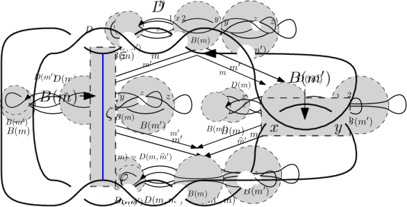
Figure 15: Two feasible moves $m=\{x\}_{\rm{I}^{-}}$ and $m^{\prime}=\{y,z\}_{\rm{II}^{-}}$ in a diagram $D$ with disjoint private balls. After applying the two moves in any order, we get the same diagram.

In example, on Figure 15, the two used moves have the same combinatorial description in both orders. Namely $m$ is feasible in $D(m^{\prime})$, $m^{\prime}$ is feasible in $D(m)$ and $D(m,m^{\prime})=D(m^{\prime},m)$. However, this need not be true in general even if $B(m)$ and $B(m^{\prime})$ are disjoint. An example of such behavior is given on Figure 16. Thus, we will sometimes need to introduce a new name for a move after swapping (for example $\widehat{m}^{\prime}$ on Figure 16). But this is essentially only a notational problem.

Figure 16: Two feasible moves $m=\{x,y\}_{\rm{II}^{-}}$ and $m^{\prime}=(\overrightarrow{\varepsilon},+)_{\rm{I}^{+}}$in a diagram $D$ with disjoint private balls. After applying $m$, the move $m^{\prime}$ is not feasible anymore but instead of it we have to use a combinatorially different move $\widehat{m}^{\prime}=(\overrightarrow{\widehat{\varepsilon}},+)_{\rm{I}^{+}}$ to get the same result. (Note that the edge $\varepsilon$ is different from $\widehat{\varepsilon}$.)

Now we provide the main technical lemma which allows swapping the moves.

Lemma 10.

Let $D$ be a diagram of a knot and $S$ be a set of crossings in $D$. Let $m=\{x,y\}_{\rm{II}^{-}}$ be a $\rm{II}^{-}$ move in $D$, greedy with respect to $S$. Let $m^{\prime}$ be a feasible move for the pair $(D,S)$ which avoids $\{x,y\}$. Then there is a move $\widehat{m}^{\prime}$ feasible in $D(m)$ of same type as $m^{\prime}$ and the following conditions hold:

1. $m$ is greedy in $D(m^{\prime})$ with respect to $S(m^{\prime})$, in particular $m$ is feasible in $(D,S)(m^{\prime})$

2. $\widehat{m}^{\prime}$ is feasible in $(D,S)(m)$; and

3. $(D,S)(m,\widehat{m}^{\prime})=(D,S)(m^{\prime},m)$.

Proof.

We will use case analysis according to the type of $m^{\prime}$ in order to show that the private balls $B(m)$ and $B(m^{\prime})$ can be chosen to be disjoint and we will perform the moves only inside these private balls. As soon as we get this, let $\widehat{m}^{\prime}$ be the move in $D(m)$ which performs the same change inside $B(m^{\prime})$ as $m$ in $D$. We also observe that the move which performs the same change inside $B(m)$ in $D(m^{\prime})$ as $m$ in $D$ is again $m$, because a $\rm{II}^{-}$ move is uniquely determined by the crossings removed by this move. Then we get that $m$ is feasible in $D(m^{\prime})$ and $D(m,\widehat{m}^{\prime})=D(m^{\prime},m)$, which will be our first step in the proof.

Now, let us distinguish cases according to the type of $m^{\prime}$.

We start with the case that $m^{\prime}$ is a $\rm{I}^{-}$ move, $\rm{II}^{-}$ move or a $\rm{III}$ move. The condition that $m^{\prime}$ avoids $\{x,y\}$ implies that the circle of $c(m)$ is disjoint from the circle $c(m^{\prime})$ of $m^{\prime}$. (Recall that $c(m)$ is depicted at Figure 8.) In addition, these two circles cannot be nested as $D$ does not pass through the open disks bounded by them. Thus $B(m)$ can be chosen so that it contains $c(m)$, the disk bounded by $c(m)$ and a small neighborhood of $c(m)$. Similarly, $B(m^{\prime})$ can be chosen so that it contains $c(m^{\prime})$, the disk bounded by $c(m^{\prime})$ and a small neighborhood of $c(m^{\prime})$. Because $c(m)$ and $c(m^{\prime})$ have strictly positive distance, the ‘small neighborhoods’ above can be chosen sufficiently small so that $B(m)$ and $B(m^{\prime})$ are disjoint.

Next, let us consider the case that $m^{\prime}$ is a $\rm{I}^{+}$ move performed on an edge $\varepsilon^{\prime}$. Because $m^{\prime}$ avoids $\{x,y\}$ we get that the image of the edge $\varepsilon^{\prime}$ is disjoint from $c(m)$. Thus we can chose $B(m)$ as in the previous case so that it avoids $\varepsilon^{\prime}$ while it is sufficient to pick $B(m^{\prime})$ as a small neighborhood of arbitrary point on $\varepsilon^{\prime}$ disjoint from $B(m)$.

Finally, let us consider the case that $m^{\prime}$ is a ${\rm{II}^{+}}$ move performed on edges $\varepsilon^{\prime}$ and $\varphi^{\prime}$, not necessarily distinct. Because $m^{\prime}$ avoids $\{x,y\}$ we get that the image of the edges $\varepsilon^{\prime}$ and $\varphi^{\prime}$ is disjoint from $c(m)$. Following the description of feasible ${\rm{II}^{+}}$ moves, let $\zeta^{\prime}$ be a topological arc (inside a face of the diagram, except the endpoints) connecting $\varepsilon^{\prime}$ and $\varphi^{\prime}$ along which the move $m^{\prime}$ is performed. Then $\zeta^{\prime}$ is also disjoint from $c(m)$. Consequently, we can choose $B(m)$ as above so that it is disjoint from $\zeta^{\prime}$ while $B(m^{\prime})$ is chosen in a small neighborhood of $\zeta^{\prime}$ so that it is disjoint from $B(m)$.

This finishes the initial case analysis, thus we know that $m$ is feasible in $D(m^{\prime})$ and $D(m,\widehat{m}^{\prime})=D(m^{\prime},m)$, which will be our first step in the proof. In order to finish the proof, we observe that $S(m)=S$ because $m$ is greedy in $D$ with respect to $S$ and we distinguish whether $m^{\prime}$ is greedy or special in $D$ with respect to $S$.

If $m^{\prime}$ is greedy, then it is a $\rm{II}^{-}$ move. We get that $S(m^{\prime})=S$. Say that $m^{\prime}$ removes crossings $w,z$ distinct from $x,y$. Then $S$ does not contain $w,z$ because $m^{\prime}$ is greedy. Consequently both $m$ and $\widehat{m}^{\prime}$ are greedy with respect to $S=S(m)=S(m^{\prime})$ (this proves (i) and (ii)), therefore both $(m,\widehat{m}^{\prime})$ and $(m^{\prime},m)$ are feasible in $(D,S)$ and $S(m,\widehat{m}^{\prime})=S(m^{\prime},m)=S$ by Lemma 6. Together with $D(m,\widehat{m}^{\prime})=D(m^{\prime},m)$ this proves (iii).

Now, let us assume that $m^{\prime}$ is special. Because neither $x$ nor $y$ belongs to $X(m^{\prime})$ (as $m^{\prime}$ avoids $\{x,y\}$), we get that $m$ is greedy in $D(m^{\prime})$ with respect to $S(m^{\prime})$ which in particular gives (i). Consequently $(m^{\prime},m)$ is feasible for $(D,S)$ and $S(m^{\prime},m)=S\triangle X(m^{\prime})$ by Lemma 6. On the other hand, $\widehat{m}^{\prime}$ is special in $D(m)$ with respect to $S(m)$ as $S(m)=S$ (and from the definition of $\widehat{m}^{\prime}$) which in particular gives (ii). We also get that $X(m^{\prime})=X(\widehat{m}^{\prime})$ as they are of the same type and they affect the same set of crossings. Altogether, $(m,\widehat{m}^{\prime})$ is feasible for $(D,S)$ and $S(m,\widehat{m}^{\prime})=S\triangle X(\widehat{m}^{\prime})=S\triangle X(m^{\prime})$ by Lemma 6. Thus we checked $S(m^{\prime},m)=S(m,\widehat{m}^{\prime})$. Together with $D(m^{\prime},m)=D(m,\widehat{m}^{\prime})$, this gives (iii). ∎

Corollary 11.

Let $D$ be a diagram, $S$ be a set of crossings in $D$, $\ell\geq 2$, and $(m_{1},\dots,m_{\ell})$ be a feasible sequence of Reidemeister moves for the pair $(D,S)$. Assume that $m_{\ell}$ is a $\rm{II}^{-}$ move which is also feasible and greedy in $D$ with respect to $S$. Then there is a sequence of Reidemester moves $(m_{\ell},\widehat{m}_{1},\dots,\widehat{m}_{\ell-1})$ feasible for $(D,S)$ such that

1. $(D,S)(m_{1},\dots,m_{\ell})=(D,S)(m_{\ell},\widehat{m}_{1},\dots,\widehat{m}_{\ell-1})$; and

2. $w(m_{i})=w(\widehat{m}_{i})$ for $i\in[\ell-1]$.

Proof.

We will prove the corollary by induction in $\ell$. If $\ell=2$, then this immediately follows from Lemma 10 used with $m=m_{2}$ and $m^{\prime}=m_{1}$ obtaining $\widehat{m}_{1}:=\widehat{m}^{\prime}$. Note that $w(m_{1})=w(\widehat{m}_{1})$ because $m_{1}$ and $\widehat{m}_{1}$ are of the same type. Thus we may assume that $\ell\geq 3$.

Let $D^{\prime}:=D(m_{1})$ and $S^{\prime}:=S(m_{1})$. We get that $(m_{2},\dots,m_{\ell})$ is a feasible sequence for $(D^{\prime},S^{\prime})$. We first apply Lemma 10 in $D$ with $m=m_{\ell}$ and $m^{\prime}=m_{1}$, at this moment, we only deduce that $m_{\ell}$ is feasible in $D^{\prime}$ and greedy with respect to $S^{\prime}$ from the item (i) of Lemma 10. We also get that $(m_{2},\dots,m_{\ell})$ is feasible for $(D^{\prime},S^{\prime})$ because $(m_{1},\dots,m_{\ell})$ is feasible for $(D,S)$. Therefore, by induction, there is a sequence $(m_{\ell},\widehat{m}_{2},\dots,\widehat{m}_{\ell-1})$ feasible for $(D^{\prime},S^{\prime})$ such that

1. $(D^{\prime},S^{\prime})(m_{2},\dots,m_{\ell})=(D^{\prime},S^{\prime})(m_{\ell},\widehat{m}_{2},\dots,\widehat{m}_{\ell-1})$; and

2. $w(m_{i})=w(\widehat{m}_{i})$ for $i\in\{2,\dots,\ell-1\}$.

Now, for checking (i) and (ii), we use Lemma 10 in its full strength, again applied with $m=m_{2}$ and $m^{\prime}=m_{1}$. Let $\widehat{m}_{1}:=\widehat{m}^{\prime}$, using the notation of the lemma. We immediately deduce (ii) from (ii’) as $m_{1}$ and $\widehat{m}_{1}$ are of the same type. We also get $(D,S)(m_{1},m_{\ell})=(D,S)(m_{\ell},\widehat{m}_{1})$ from item (iii) of Lemma 10. Using this and (i’) we get

$$(D,S)(m_{1},\dots,m_{\ell}) =(D^{\prime},S^{\prime})(m_{2},\dots,m_{\ell})$$

$$=(D^{\prime},S^{\prime})(m_{\ell},\widehat{m}_{2},\dots,\widehat{m}_{\ell-1})$$

$$=(D,S)(m_{1},m_{\ell})(\widehat{m}_{2},\dots,\widehat{m}_{\ell-1})$$

$$=(D,S)(m_{\ell},\widehat{m}_{1})(\widehat{m}_{2},\dots,\widehat{m}_{\ell-1})$$

$$=(D,S)(m_{\ell},\widehat{m}_{1},\widehat{m}_{2},\dots,\widehat{m}_{\ell-1})$$

which verifies (i); note that the computations also show that the sequence $(m_{\ell},\widehat{m}_{1},\widehat{m}_{2},\dots,\widehat{m}_{\ell-1})$ is feasible for $(D,S)$. ∎

We also need one more swapping lemma for two consecutive moves (and one more auxiliary move).

Lemma 12.

Let $D$ be a diagram of a knot and $S$ be a set of crossings in $D$. Assume that $m=\{x,y\}_{\rm{II}^{-}}$ and $\widetilde{m}=\{x,z\}_{\rm{II}^{-}}$, with $y\neq z$, are feasible $\rm{II}^{-}$ moves in $D$, greedy with respect to $S$. Assume also that $m^{\prime}$ is a feasible move for $(D(m),S(m))$ which avoids $\{z\}$. Then there is a move $\widehat{m}^{\prime}$ feasible for $(D,S)$ of same type as $m^{\prime}$ such that the following conditions hold:

1. $m$ is feasible for $(D,S)(\widehat{m}^{\prime})$;

2. $(D,S)(m,m^{\prime})=(D,S)(\widehat{m}^{\prime},m)$.

Proof.

Many steps in the proof will be similar to the proof of Lemma 10; however, we have to be careful with the analogy as the assumptions are different. Our first aim is again to get the private balls $B(m)$ and $B(m^{\prime})$ disjoint by case analysis according to the type of $m^{\prime}$. Note that this makes sense in particular when focusing to diagram $D(m)$ where $B(m)$ appears because $D(m)$ was obtained by performing $m$ while $B(m^{\prime})$ appears because $m^{\prime}$ is feasible in $D(m)$. Once we get that $B(m)$ and $B(m^{\prime})$ are disjoint, then we know that there is a move $\widehat{m}^{\prime}$ in $D$ which performs the same change inside $B(m^{\prime})$ as the move $m^{\prime}$ in $D(m)$. Similarly, there is a move $\widehat{m}$ in $D(\widehat{m}^{\prime})$ which performs the same change as $m$ in $D$. Then we get $D(m,m^{\prime})=D(\widehat{m}^{\prime},\widehat{m})$. In addition, similarly as in the proof of Lemma 10, we get $m=\widehat{m}$ for free because $m$ is a $\rm{II}^{-}$ move.

Before we start the case analysis according to the type of $m^{\prime}$, we start with some common preliminaries.

Let us pick the private ball $B(m)$ arbitrarily so that it meets the diagram $D$ as in Figure 17, left. Let $\alpha$ and $\beta$ be two arcs in $D$ such that $B(m)$ intersects (the image of) $D$ in (the images of) $\alpha$ and $\beta$. Let $\alpha(m)$ and $\beta(m)$ be the arcs in $D(m)$ coming from $\alpha$ and $\beta$ after applying the move $m$. We also define $\varepsilon(m)$ and $\varphi(m)$ as the edges of $D(m)$ which contain $\alpha(m)$ and $\beta(m)$. An important observation is that one of the endpoints of each of $\varepsilon(m)$ and $\varphi(m)$ is $z$. Indeed, because $\widetilde{m}=\{x,z\}_{\rm{II}^{-}}$ is feasible in $D$, there are two edges $\widetilde{\varepsilon}$, $\widetilde{\varphi}$ in $D$ connecting $x$ and $z$; see Figure 17, right. Then, one of them, say $\widetilde{\varepsilon}$, partially coincides with $\alpha$ while the other one, $\widetilde{\varphi}$, partially coincides with $\beta$. It follows that $\varepsilon(m)$ contains the image of the arc obtained from $\widetilde{\varepsilon}$ after performing $m$. In particular, $\varepsilon(m)$ contains $z$ which implies that $z$ is an endpoint of $\varepsilon(m)$. Similarly, $z$ is an endpoint of $\varphi(m)$. Note also that if we perform the move $m$ on $D$ as on  Figure 17, left, then $\widetilde{\varepsilon}$ and $\widetilde{\varphi}$ as well as $\varepsilon(m)$ and $\varphi(m)$ have to leave $B(m)$ from the ‘upper side’ as on Figure 17, right, because $z\neq y$. Now we start distinguishing the cases.

Figure 17: Performing the move $m$.

We again start with the case that $m^{\prime}$ is a $\rm{I}^{-}$ move, $\rm{II}^{-}$ move or a $\rm{III}$ move. In this case, we want to check that $c(m^{\prime})$ is disjoint from (the images of) $\alpha(m)$ and $\beta(m)$. However, if $c(m^{\prime})$ meets, for example $\alpha(m)$, then it has to contain (the image of) $\varepsilon(m)$ and in particular $z$. But this is impossible as $m^{\prime}$ avoids $z$. Therefore, $c(m^{\prime})$ has positive distance from $\alpha(m)$ and $\beta(m)$ which also implies that it has positive distance from $B(m)$. In addition, $B(m)$ cannot be contained in the open disk bounded by $c(m^{\prime})$ because $D(m)$ does not pass through this disk. Therefore, $B(m^{\prime})$ can be chosen disjoint from $B(m)$ so that it contains this disk and a small neighborhood of $c(m^{\prime})$.

Next, let us consider the case that $m^{\prime}$ is a $\rm{I}^{+}$ move; say $m^{\prime}=(\overrightarrow{\varepsilon}^{\prime},\sigma^{\prime})_{\rm{I}^{+}}$. Because $m^{\prime}$ avoids $\{z\}$, we get that the image of the edge $\varepsilon^{\prime}$ is disjoint from (the images of) $\alpha(m)$ and $\beta(m)$ (because they are in edges containing $z$). Thus it is possible to pick $B(m^{\prime})$ as a small neighborhood of an arbitrary point on $\overrightarrow{\varepsilon}^{\prime}$ disjoint from $B(m)$.

Finally, let us consider the case that $m^{\prime}$ is a ${\rm{II}^{+}}$ move; say $m^{\prime}=(\overrightarrow{\varepsilon}^{\prime},\overrightarrow{\varphi}^{\prime},w^{\prime},o^{\prime})_{{\rm{II}^{+}}}$. Because $m^{\prime}$ avoids $\{z\}$ we get that the image of the edges $\overrightarrow{\varepsilon}^{\prime}$ and $\overrightarrow{\varphi}^{\prime}$ is disjoint from $\varepsilon(m)$ and $\varphi(m)$. Following the description of feasible ${\rm{II}^{+}}$ moves, let $\zeta^{\prime}$ be a topological arc (inside a face of the diagram $D(m)$, except the endpoints) connecting $\overrightarrow{\varepsilon}^{\prime}$ and $\overrightarrow{\varphi}^{\prime}$ along which the move $m^{\prime}$ is performed. We want to show that, up to isotopy, $\zeta^{\prime}$ can be chosen so that it is disjoint with $B(m)$. Indeed we can perform an (ambient) isotopy which keeps the diagram $D(m)$ fixed and which maps $B(m)$ to a ball $\bar{B}(m)$ inside a small neighborhood of the union (of the images) of $\overrightarrow{\varepsilon}(m)$ and $\overrightarrow{\varphi}(m)$ so that $\bar{B}(m)$ and $\zeta^{\prime}$ are disjoint; see Figure 18. This isotopy is indeed possible because $\overrightarrow{\varepsilon}(m)$ and $\overrightarrow{\varphi}(m)$ leave $B(m)$ from the ‘upper side’ as we argued above in the case analysis.

Now, if we want to get $\zeta^{\prime}$ disjoint with $B(m)$, up to isotopy, it is sufficient to apply the inverse of this isotopy to $\zeta^{\prime}$. Once we have $\zeta^{\prime}$ disjoint with $B(m)$, we can pick $B(m^{\prime})$ as a small neighborhood of $\zeta^{\prime}$, disjoint with $B(m)$. This finishes the proof.

Figure 18: Isotoping $B(m)$ so that it avoids $\zeta^{\prime}$.

This finishes our initial case analysis, thus we get that $\widehat{m}^{\prime}$ is feasible in $D$, $m$ is feasible in $D(\widehat{m}^{\prime})$ and $D(m,m^{\prime})=D(\widehat{m}^{\prime},m)$. It remains to check that these properties are kept also with respect to $S$.

First, we realize that $S=S(m)$ due to 5 because $m$ is greedy in $D$ with respect to $S$. Next, we distinguish whether $m^{\prime}$ is greedy or special with respect to $S(m)$.

First assume that $m^{\prime}$ is greedy, in particular a $\rm{II}^{-}$ move. Let $m^{\prime}=\{x^{\prime},y^{\prime}\}_{\rm{II}^{-}}$. Then we get that $x^{\prime},y^{\prime}\not\in S(m)=S$. Thus, $\widehat{m}^{\prime}$ is also greedy (with respect to $S$) as it removes the same crossings. In particular $\widehat{m}^{\prime}$ is feasible for $(D,S)$. By another application of 5, we get $S(\widehat{m}^{\prime})=S$. Therefore $m$ is greedy in $D(\widehat{m}^{\prime})$ with respect to $S(\widehat{m}^{\prime})$, which gives (i). In addition $S(m,m^{\prime})=S=S(\widehat{m}^{\prime},m)$ by Lemma 6 which gives (ii), using also $D(m,m^{\prime})=D(\widehat{m}^{\prime},m)$.

Now, let us assume that $m^{\prime}$ is special. If $\widehat{m}^{\prime}$ is a $\rm{I}^{-}$, $\rm{II}^{-}$, or a $\rm{III}$ move, we deduce that $\widehat{m}^{\prime}$ is special in $D$ with respect to $S$ because it removes/affects the same crossings as $m^{\prime}$ and $S=S(m)$. If $\widehat{m}^{\prime}$ is a $\rm{I}^{+}$ or a ${\rm{II}^{+}}$ move, we deduce that $\widehat{m}^{\prime}$ is special in $D$ with respect to $S$ as soon as we check that the endpoints of the edge(s) on which is $\widehat{m}^{\prime}$ performed belong to $S$. However, this edge/these edges cannot belong to the private ball $B(m)$ by our earlier case analysis (we have obtained disjointess with $\alpha(m)$ and $\beta(m)$). In particular, this edge/these edges are not affected by $m$ when performed in $D$, which shows that their endpoints have to belong to $S$ (as $m^{\prime}$ is special in $D(m)$ with respect to $S(m)=S$). In particular, in all cases according to the type of $m^{\prime}$ we get that $\widehat{m}^{\prime}$ is feasible with respect to $(D,S)$ and we also get $X(m^{\prime})=X(\widehat{m}^{\prime})$ and $x,y\not\in X(m^{\prime})$. By 5, we get $S(\widehat{m}^{\prime})=S\triangle X(\widehat{m}^{\prime})=S\triangle X(m^{\prime})$. This shows that $m$ is greedy in $D(\widehat{m}^{\prime})$ with respect to $S(\widehat{m}^{\prime})$ as $x,y\not\in S$ and $x,y\not\in X(m^{\prime})$. In particular, this imples (i). Finally, by Lemma 6, we get $S(m,m^{\prime})=S\triangle X(m^{\prime})=S\triangle X(\widehat{m}^{\prime})=S(\widehat{m}^{\prime},m)$. Together with $D(m,m^{\prime})=D(\widehat{m}^{\prime},m)$, this gives (ii). ∎

Corollary 13.

Let $D$ be a diagram, $S$ be a set of crossings in $D$, $\ell\geq 2$ and $(m_{1},\dots,m_{\ell})$ be a feasible sequence of moves for $(D,S)$. Assume that $m_{1}=\{x_{1},y_{1}\}_{\rm{II}^{-}}$ and $m_{\ell}=\{x_{\ell},y_{\ell}\}_{\rm{II}^{-}}$ are $\rm{II}^{-}$ moves where $x_{1},y_{1},x_{\ell},y_{\ell}\not\in S$ (in particular $m_{1}$ is greedy in $D$ with respect to $S$). Finally, assume also that $\{x_{1},x_{\ell}\}_{\rm{II}^{-}}$ is a feasible Reidemeister move for $(D,S)$ (again, it must be greedy). Then, there is a feasible sequence $(\widehat{m}_{2},\widehat{m}_{3},\dots,\widehat{m}_{\ell-1},m_{1})$ of moves for $(D,S)$ such that

1. $(D,S)(m_{1},\dots,m_{\ell-1})=(D,S)(\widehat{m}_{2},\widehat{m}_{3},\dots,\widehat{m}_{\ell-1},m_{1})$; and

2. $w(m_{i})=w(\widehat{m}_{i})$ for $i\in\{2,\dots,\ell-1\}$.

Proof.

We will prove the corollary by induction in $\ell$. For $\ell=2$, there is nothing to prove (considering $m_{2},\dots,m_{\ell-1}$ as an empty sequence).

Let us assume $\ell\geq 3$. Let us apply Lemma 12 with $m=m_{1}$ and $m^{\prime}=m_{2}$, obtaining $\widehat{m}_{2}:=\widehat{m}^{\prime}$. In particular, we get $w(m_{2})=w(\widehat{m}_{2})$, verifying (ii) for $i=2$.

We also know that $\widehat{m}_{2}$ is feasible for $(D,S)$. Let $D^{\prime}:=D(\widehat{m}_{2})$ and $S^{\prime}=S(\widehat{m}_{2})$. Then $m_{1}$ is feasible for $(D^{\prime},S^{\prime})$ by item (i) of  Lemma 12 and we get

$$(D,S)(m_{1},m_{2})=(D,S)(\widehat{m}_{2},m_{1})=(D^{\prime},S^{\prime})(m_{1})$$ (1)

by item (ii) of Lemma 12. This together gives that the sequence $(\widehat{m}_{2},m_{1},m_{3},m_{4},\dots,m_{\ell})$ is feasible for $(D,S)$, therefore $(m_{1},m_{3},m_{4},\dots,m_{\ell})$ is feasible for $(D^{\prime},S^{\prime})$. We want to check the induction assumptions for $D^{\prime}$ and this sequence. We need to check:

• $m_{1}$ is feasible for $(D^{\prime},S^{\prime})$. This follows from item (i) of  Lemma 12.

• $x_{1},y_{1},x_{\ell},y_{\ell}$ do not belong to $S^{\prime}$. This follows from the assumption $x_{1},y_{1},x_{\ell},y_{\ell}\not\in S$ and 5. Indeed if $\widehat{m}_{2}$ is greedy, then $S^{\prime}=S$ and there is nothing to do. Thus we may assume that $\widehat{m}_{2}$ is special and $S^{\prime}=S\triangle X(\widehat{m}_{2})$. Then it is sufficient to check that none of $x_{1},y_{1},x_{\ell},y_{\ell}$ belongs to $X(\widehat{m}_{2})$. If $\widehat{m}_{2}$ is a $\rm{I}^{-}$ move, $\rm{II}^{-}$ move or a $\rm{III}$ move, then $X(\widehat{m}_{2})\cap\{x_{1},y_{1},x_{\ell},y_{\ell}\}$ is empty because $\widehat{m}_{2}$ is special with respect to $S$, thus it cannot remove/affect a crossing not in $S$. If $\widehat{m}_{2}$ is a $\rm{I}^{+}$ move or a ${\rm{II}^{+}}$ move, then $X(\widehat{m}_{2})$ is the set of crossing created by $\widehat{m}_{2}$. The crossings $x_{1},y_{1},x_{\ell}$ cannot be created by $\widehat{m}_{2}$ because they are already present in $D$ (due to feasible moves $m_{1}$ and $m_{\ell}$). However, $y_{\ell}$ is a crossing of $D$ as well as it is removed by $m_{\ell}$ while it cannot be created during the sequence $(m_{1},\dots,m_{\ell-1})$ because this would make $m_{\ell}$ special (with respect to $S(m_{1},\dots,m_{\ell-1})$) contradicting that $x_{\ell}$ does not belong to $S$.

• $\{x_{1},x_{\ell}\}_{\rm{II}^{-}}$ is a feasible Reidemeister move in $D^{\prime}$. This follows from Lemma 10(i) applied to $(D,S)$ with $m=\{x_{1},x_{\ell}\}_{\rm{II}^{-}}$ and $m^{\prime}=\widehat{m}_{2}$. For this, we need to check that $\widehat{m}_{2}$ avoids $\{x_{1},x_{\ell}\}$.

  This is almost for free if $\widehat{m}_{2}$ is a special move in $D^{\prime}$ with respect to $S^{\prime}$, because in this case $\widehat{m}_{2}$ avoids crossings not in $S^{\prime}$ by the definition of special move. In particular, it avoids $x_{1}$ and $x_{\ell}$ which are not in $S$ because they can be removed by the greedy $\{x_{1},x_{\ell}\}$ move in $D$ with respect to $S$ — therefore, they do not belong to $S^{\prime}$ either.

  However, it is also easy to check that $\widehat{m}_{2}$ avoids $\{x_{1},x_{\ell}\}$ if $\widehat{m}_{2}$ is greedy, in particular a $\rm{II}^{-}$ move. We know that $m_{2}$ and $\widehat{m}_{2}$ are of the same type, thus $m_{2}$ is greedy as well. In addition, from $D(m_{1},m_{2})=D(\widehat{m}_{2},m_{1})$ (which is a special case of (1)), we get that $\widehat{m}_{2}$ has to remove the same crossings as $m_{2}$, thus $\widehat{m}_{2}=m_{2}$. Then $m_{2}$ avoids $x_{1}$ because $(m_{1},m_{2})$ is a feasible sequence in $D$ and $m_{1}$ removes $x_{1}$ and $m_{2}$ avoids $x_{\ell}$ because $(m_{1},\dots,m_{\ell})$ is a feasible sequence in $D$ and thus $x_{\ell}$, which is removed by $m_{\ell}$ has to persist until $D(m_{1},\dots,m_{\ell-1})$.

Therefore, by induction we get a feasible sequence $(\widehat{m}_{3},\widehat{m}_{4},\dots,\widehat{m}_{\ell-1},m_{1})$ for $(D^{\prime},S^{\prime})$ and

$$(D^{\prime},S^{\prime})(m_{1},m_{3},m_{4},\dots,m_{\ell-1})=(D^{\prime},S^{\prime})(\widehat{m}_{3},\widehat{m}_{4},\dots,\widehat{m}_{\ell-1},m_{1}).$$ (2)

In particular, $w(m_{i})=w(\widehat{m}_{i})$ for $i\in\{3,\dots,\ell-1\}$ by induction which together with $w(m_{2})=w(\widehat{m}_{2})$ verifies item (ii) of this lemma.

For (i), by (1) and (2) we obtain

$$(D,S)(m_{1},\dots,m_{\ell-1}) =(D,S)(m_{1},m_{2})(m_{3},\dots,m_{\ell-1})$$

$$=(D^{\prime},S^{\prime})(m_{1},m_{3},m_{4},\dots,m_{\ell-1})$$

$$=(D^{\prime},S^{\prime})(\widehat{m}_{3},\widehat{m}_{4},\dots,\widehat{m}_{\ell-1},m_{1})$$

$$=(D,S)(\widehat{m}_{2},\widehat{m}_{3},\dots,\widehat{m}_{\ell-1},m_{1})$$

as required, which also shows feasibility of the sequence $(\widehat{m}_{2},\widehat{m}_{3},\dots,\widehat{m}_{\ell-1},m_{1})$ for $(D,S)$. ∎

Lemma 14.

Let $D$ be a diagram of a knot and let $m=\{x,y\}_{\rm{II}^{-}}$, $\widetilde{m}=\{x,z\}_{\rm{II}^{-}}$ be two feasible Reidemeister moves in $D$ where $y\neq z$. Assume also that $m^{\prime}=\{w,z\}_{\rm{II}^{-}}$ is feasible in $D(m)$ with $x,y,z,w$ mutually distinct. Then

1. $\widetilde{m}^{\prime}=\{w,y\}_{\rm{II}^{-}}$ is feasible in $D(\widetilde{m})$; and

2. $D(m,m^{\prime})=D(\widetilde{m},\widetilde{m}^{\prime})$.

Proof.

We will provide a direct argument. However, as an alternative proof, the reader may want to check that there are combinatorially only four options (up to a mirror image) for how $x,y,z,$ and $w$ can be arranged in the diagram, each of them yielding the required conclusion; see Figure 19.

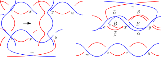
Figure 19: Four options how may $x,y,z$ and $w$ be arranged.

Let $\alpha$ and $\beta$ be the edges connecting $x$ and $y$ in $D$ along which the move $m$ is performed. Similarly, let $\widetilde{\alpha}$ and $\widetilde{\beta}$ be the edges connecting $x$ an $z$ along which the move $\widetilde{m}$ is performed. Let us also assume that $\alpha$ and $\widetilde{\alpha}$ enter $x$ as overpasses and $\beta$ and $\widetilde{\beta}$ as underpasses. We also know that $\alpha,\beta,\widetilde{\alpha}$ and $\widetilde{\beta}$ are four distinct edges because $y\neq z$. Finally, because the ‘bigon’ $B$ between $\alpha$ and $\beta$ is empty as well as the ‘bigon’ $\widetilde{B}$ between $\widetilde{\alpha}$ and $\widetilde{\beta}$ is empty, and those two bigons touch at $x$, there is a unique way, up to an isotopy and a mirror image, how this portion of diagram may look like; see Figure 20.

Figure 20: Left: Portion of the diagram $D$ around $x$, $y$ and $z$. Right: results after applying $m$ and $\widetilde{m}$.

Now, when we compare $D(m)$ and $D(\widetilde{m})$ we get the same diagram up to isotopy and relabelling $z\leftrightarrow y$. This in particular gives (i): if $m^{\prime}=\{w,z\}_{\rm{II}^{-}}$ is feasible in $D(m)$, then after relabelling, we get that $\widetilde{m}^{\prime}=\{w,y\}_{\rm{II}^{-}}$ is feasible in $D(\widetilde{m})$.

In addition, because of relabelling, performing $m^{\prime}$ in $D(m)$ and $\widetilde{m}^{\prime}$ in $D(\widetilde{m})$ yields the same diagrams $D(m,m^{\prime})$ and $D(\widetilde{m},\widetilde{m}^{\prime})$ with respect to our combinatorial description of diagrams. Indeed, if $D$ contains only four crossings $x$, $y$, $z$ and $w$, then $D(m,m^{\prime})=D(\widetilde{m},\widetilde{m}^{\prime})$ is the diagram without crossings. If $D$ contains more than four crossings, then we know that the sets of crossings is the same in $D(m,m^{\prime})$ and $D(\widetilde{m},\widetilde{m}^{\prime})$. Thus it remains to check that we also get exactly same edges (that is we get the same combinatorial description of edges). Let $\varepsilon^{\prime}=(v_{1},v_{2},n_{1},n_{2})$ be an edge in $D(m,m^{\prime})$. Its pre-image before performing $m^{\prime}$ is an arc $\varepsilon$ in $D(m)$ connecting $v_{1}$ and $v_{2}$ entering $v_{1}$ in strand $n_{1}$ and entering $v_{2}$ in strand $n_{2}$, possibly passing through $z$ and $w$ but not through other crossings of $D(m)$. Because of isotopy between $D(m)$ and $D(\widetilde{m})$, this arc is isotoped to an arc $\widetilde{\varepsilon}$ in $D(\widetilde{m})$ again connecting $v_{1}$ and $v_{2}$ entering $v_{1}$ in strand $n_{1}$ and entering $v_{2}$ in strand $n_{2}$, possibly passing through $y$ and $w$ but not through other crossings of $D(\widetilde{m})$. After performing the move $\widetilde{m}^{\prime}$, we get the edge $(v_{1},v_{2},n_{1},n_{2})$ in $D(\widetilde{m},\widetilde{m}^{\prime})$ out of this arc. Analogously, by reverting this argument, an edge in $D(\widetilde{m},\widetilde{m}^{\prime})$ induces the same edge in $D(m,m^{\prime})$. ∎

Now, we have all tools to prove Theorem 9. For reader’s convenience, we recall the statement.

Theorem 9.

Let $D$ be a diagram of a knot and $S$ be a set of crossings in $D$. Let $(m_{1},\dots,m_{\ell})$ be a feasible sequence of Reidemeister moves for $(D,S)$, inducing an untangling of $D$ with defect $k$. Let $\widetilde{m}$ be a greedy move in $D$ with respect to $S$. Then there is a feasible sequence of Reidemeister moves for $(D,S)$ starting with $\widetilde{m}$ and inducing an untangling of $D$ with defect $k$.

Proof of Theorem 9.

First, let us assume that $\widetilde{m}=m_{j}$ for some $j\in[\ell]$. If $j=1$, there is nothing to prove, thus we may assume $j\geq 2$. Then, by using Corollary 11 on the sequence $(m_{1},\dots,m_{j})$, we get a sequence of moves $(m_{j},\widehat{m}_{1},\dots,\widehat{m}_{j-1})$ feasible for $(D,S)$. By item (i) of Corollary 11, the sequence $(m_{j},\widehat{m}_{1},\dots,\widehat{m}_{j-1},m_{j+1},\dots,m_{\ell})$ is also feasible for $(D,S)$ and induces an untangling of $D$. By item (ii) of Corollary 11 and Lemma 3, the defect of this sequence equals $k$, and that is what we need.

Thus it remains to consider the case where $\widetilde{m}\neq m_{j}$ for every $j\in[\ell]$. Because, $\widetilde{m}$ is greedy, it is in particular a $\rm{II}^{-}$ move, say $\widetilde{m}=\{x,z\}_{\rm{II}^{-}}$. Because the final diagram $D(m_{1},\dots,m_{\ell})$ contains no crossings, the crossings $x$ and $z$ have to be removed by some moves in the sequence $(m_{1},\dots,m_{\ell})$. Say that a move $m_{i}$ removes $x$ and $m_{j}$ removes $z$. Since we assumed that $\widetilde{m}$ is greedy with respect to $S$, we get $x,z\notin S$. In particular $x\notin S(m_{1},\dots,m_{i-1})$ by Lemma 6 ($x$ never belongs to any $X(m_{i^{\prime}})$ for $i^{\prime}<i$ as it is not removed earlier), thus $m_{i}$ has to be greedy move in $D(m_{1},\dots,m_{i-1})$ with respect to $S(m_{1},\dots,m_{i-1})$. Similarly, $m_{j}$ is greedy in $D(m_{1},\dots,m_{j-1})$ with respect to $S(m_{1},\dots,m_{j-1})$. Because we assume that $\widetilde{m}$ is not in the sequence $(m_{1},\dots,m_{\ell})$, we get $i\neq j$. Without loss of generality, let us assume $i<j$. Let $y$ and $w$ be such that $m_{i}=\{x,y\}_{\rm{II}^{-}}$ and $m_{j}=\{w,z\}_{\rm{II}^{-}}$. As these moves are greedy, we get $y,w\not\in S$ (again using Lemma 6).

Let $D^{\prime}:=D(m_{1},\dots,m_{i-1})$ and $S^{\prime}:=S(m_{1},\dots,m_{i-1})$. By Corollary 13, applied to $D^{\prime}$, $S^{\prime}$ and the sequence $(m_{i},\dots,m_{j})$ feasible for $(D^{\prime},S^{\prime})$, we get another sequence $(\widehat{m}_{i+1},\dots,\widehat{m}_{j-1},m_{i})$ feasible for $(D^{\prime},S^{\prime})$. By item (i) of Corollary 13, we get that $(\widehat{m}_{i+1},\dots,\widehat{m}_{j-1},m_{i},m_{j},\dots,m_{\ell})$ is also feasible for $(D^{\prime},S^{\prime})$.

Next, let $D^{\prime\prime}:=D^{\prime}(\widehat{m}_{i+1},\dots,\widehat{m}_{j-1})$ and $S^{\prime\prime}:=S^{\prime}(\widehat{m}_{i+1},\dots,\widehat{m}_{j-1})$. Because $x,z\notin S$, the edges between $x$ and $z$ are not used to perform $\rm{I}^{+}$ or $\rm{II}^{+}$ moves and the moves $m_{1},\dots,m_{i-1},\widehat{m}_{i+1},\dots,\widehat{m}_{j-1}$ are performed outside of the private ball $B(\widetilde{m})$. By Lemma 6, $x,z\notin S^{\prime\prime}$ and $\widetilde{m}$ is feasible in $(D^{\prime\prime},S^{\prime\prime})$. By Lemma 14 used in $D^{\prime\prime}$, we get that $\widetilde{m}^{\prime}:=\{w,y\}_{\rm{II}^{-}}$ is feasible in $(D^{\prime\prime},S^{\prime\prime})(\widetilde{m})$ and $(D^{\prime\prime},S^{\prime\prime})(m_{i},m_{j})=(D^{\prime\prime},S^{\prime\prime})(\widetilde{m},\widetilde{m}^{\prime})$. Altogether, by expanding $D^{\prime\prime}$ and $D^{\prime}$

$$(m_{1},\dots,m_{i-1},\widehat{m}_{i+1},\dots,\widehat{m}_{j-1},\widetilde{m},\widetilde{m}^{\prime},m_{j+1},\dots,m_{\ell})$$ (3)

is an untangling of $D$, feasible for $(D,S)$. We also get that the defect of this untangling is equal to $k$ by Lemma 3 and item (ii) of Corollary 13, when we used it. Note that all the moves $m_{i}$, $m_{j}$, $\widetilde{m}$ and $\widetilde{m}^{\prime}$ are $\rm{II}^{-}$ moves, thus they do not contribute to the weight.

The sequence (3) is not the desired sequence yet, because it does not start with $\widetilde{m}$. However, it contains $\widetilde{m}$, thus we can further modify this sequence to the desired sequence starting with $\widetilde{m}$ as in the first paragraph of this proof. ∎

6 W[P]-hardness

6.1 Minimum axiom set

We prove the W[P]-hardness in Theorem 2 by an FPT-reduction from Minimum axiom set defined below. It is well known that Minimum axiom set is W[P]-hard; see [FG06, Exercise 3.20] or [DF13, Lemma 25.1.3] (however, let us recall that our definition of FPT-reduction is consistent with [FG06]).

Problem (Minimum axiom set).

Input	A finite set $S$, and
	a finite set $\mathcal{R}$ which consists of pairs of form $(T,t)$ where $T\subseteq S$ and $t\in S$.
Parameter	$k$.
Question	Does there exists a subset $S_{0}\subseteq S$ of size $k$ such that if we define inductively $S_{i}$
	to be the union of $S_{i-1}$ and all $t\in S$ such that there is $T\subseteq S_{i-1}$ with $(T,t)\in\mathcal{R}$,
	then $\bigcup_{i=1}^{\infty}S_{i}=S$?

The problem above deserves a brief explanation. The elements of $S$ are called sentences and the elements of $\mathcal{R}$ are relations. A relation $(T,t)$ with $T=\{t_{1},\dots,t_{m}\}$ should be understood as an implication

$$t_{1}\wedge t_{2}\wedge\cdots\wedge t_{m}\Rightarrow t.$$

Given a set $S_{0}\subseteq S$, let us define the consequences of $S_{0}$ as $c(S_{0}):=\bigcup_{i=1}^{\infty}S_{i}$ where $S_{i}$ is defined as in the statement of the problem. Intuitively, $c(S_{0})$ consists of all sentences that can be deduced from $S_{0}$ via the relations (implications) in $\mathcal{R}$. As we work with finite sets, $c(S_{0})=S_{i}$ for some high enough $i$ (it is sufficient to take $i=|S|$). A set $A$ is a set of axioms if $c(A)=S$. Therefore, the goal of the minimum axiom set problem is to determine whether there is a set of axioms of size $k$. Note that the axiom sets are upward-closed: If $A$ is an axiom set and $A\subseteq A^{\prime}\subseteq S$, then $A^{\prime}$ is an axiom set as well.

The following boosting lemma is very useful in our reduction.

Lemma 15 (Boosting lemma).

Let $(S,\mathcal{R})$ be an input of the minimum axiom set problem (ignoring the parameter for the moment). Let $\mu\colon S\to{\mathbb{Z}}$ be a non-negative function. Given $U\subseteq S$, let $\mu(U)=\sum_{s\in U}\mu(s)$.Assume that $\mu(U)\geq 1$ for all $U$ such that $S\setminus U$ is not an axiom set. (Equivalently, $U$ meets every axiom set.) Then $\mu(S)\geq k^{*}$ where $k^{*}$ is the size of a minimum axiom set.

In our reduction, we will need to check that $\mu(S)\geq k^{*}$ for a suitable function $\mu$. However, it will be much easier to verify only $\mu(U)\geq 1$ for suitable sets $U$.

Proof.

Let $Z:=\{s\in S\colon\mu(s)=0\}$ be the zero set of $\mu$. Then $\mu(Z)=0$, thus $S\setminus Z$ is a set of axioms by the assumptions. This gives $|S\setminus Z|\geq k^{*}$ and, in addition, $\mu(S)=\mu(S\setminus Z)\geq|S\setminus Z|\geq k^{*}$ because $\mu(s)\geq 1$ for every $s\in S\setminus Z$. ∎

6.2 Construction of the reduction

Our aim is to show that there is an FPT-reduction from the Minimum axiom set to Unknotting via defect.

Preprocessing.

Let $(S,\mathcal{R},k)$ be an instance of the Minimum axiom set. We first perform a preprocessing on $(S,\mathcal{R},k)$. We repeatedly apply the following reduction rules:

1. If $(\emptyset,t)\in\mathcal{R}$, then we remove $t$ from $S$ and we replace all relations $(T^{\prime},t^{\prime})$ with $(T^{\prime}\setminus\{t\},t^{\prime})$ if $t\neq t^{\prime}$ while we remove all relations of the form $(T,t)$ from $\mathcal{R}$.

2. If there is $s\in S$ such that $\mathcal{R}$ contains no relation of a form $(T,s)$, then we replace all relations $(T^{\prime},t^{\prime})$ with $(T^{\prime}\setminus\{s\},t^{\prime})$, we remove $s$ from $S$ and we decrease $k$ by $1$.

3. If there is $(T,t)\in\mathcal{R}$ with $t\in T$, then we remove this relation $(T,t)$ from $\mathcal{R}$.

It is easy to check that the preprocessing can be done in polynomial time. In addition, it yields an equivalent instance: For (i) we easily see that such $t$ belongs to $S_{1}$ starting with arbitrary $S_{0}$. Thus $t\in c(S_{0})$ for an arbitrary $S_{0}$. Consequently, if we want to deduce that $t^{\prime}\in c(S_{0})$ via $(T^{\prime},t^{\prime})$, it is sufficient to use $(T^{\prime}\setminus\{t\},t^{\prime})$ as we already know that $t\in c(S_{0})$. We also may remove all relations $(T,t)$ from $\mathcal{R}$ as we already know that $t\in c(S_{0})$. For (ii), we see that such $s$ can never be deduced from the relations, thus such $s$ must be in every axiom set. Equivalently, if we remove $s$ from the instance, then we need to find an axiom set of size $k-1$. For (iii), we see that such a relation $(T,t)$ never yields a new sentence in $c(S_{0})$ for arbitrary $S_{0}$.

Altogether, this means that this preprocessing is an FPT-reduction. Note that in (ii) we decrease the parameter. This is consistent with the second item of our definition of FPT-reduction by setting $g^{\prime}(k)=k$.

Doubling the instance.

Now let $(S,\mathcal{R},k)$ be a preprocessed instance of the Minimum axiom set. We will need the following doubled instance: Let $\widehat{S}:=\{\widehat{s}\colon s\in S\}$ be a copy of $S$ (formally speaking, $\widehat{s}$ could be identified, for example with the pair $(s,0)$ assuming that no such pair is in $S$). Given $T=\{t_{1},\dots,t_{m}\}\subseteq S$, let $\widehat{T}:=\{\widehat{t}_{1},\dots,\widehat{t}_{m}\}$. Then we define $\widehat{\mathcal{R}}:=\{(\widehat{T},\widehat{t})\ \colon(T,t)\in\mathcal{R}\}$. Then $(S\cup\widehat{S},\mathcal{R}\cup\widehat{\mathcal{R}},2k)$ is a double of the instance $(S,\mathcal{R},k)$.

Observation 16.

The pair $(S,\mathcal{R})$ admits an axiom set of size $k$ if and only if its double $(S\cup\widehat{S},\mathcal{R}\cup\widehat{\mathcal{R}})$ admits an axiom set of size $2k$.

Proof.

If $A$ is an axiom set of size $k$ for $(S,\mathcal{R})$, then $A\cup\widehat{A}$ is an axiom set of size $2k$ for $(S\cup\widehat{S},\mathcal{R}\cup\widehat{\mathcal{R}})$. On the other hand, if $\bar{A}$ is an axiom set of size $2k$ for $(S\cup\widehat{S},\mathcal{R}\cup\widehat{\mathcal{R}})$, let $B:=\bar{A}\cap S$ and $\widehat{C}:=\bar{A}\cap\widehat{S}$. Then both $B$ and $C$ (obtained by removing the hats) are axiom sets for $(S,\mathcal{R})$. One of them has size at most $k$ (and it can be extended to size $k$ if needed). ∎

Brunnians.

A Brunnian link is a nontrivial link that becomes trivial whenever one of the link components is removed. We will use the following well known construction of a Brunnian link with $\ell\geq 2$ components. We take an untangled unknot and we interlace it with two ‘neighboring’ unknots as in Figure 21, left. We repeat this $\ell$-times and we get a Brunnian link with $\ell$ components as in Figure 21, right.

Figure 21: A Brunnian link

Gadgets.

From now on let us assume that $(S,\mathcal{R},k)$ is a preprocessed instance of the Minimum axiom set and $(S\cup\widehat{S},\mathcal{R}\cup\widehat{\mathcal{R}},2k)$ is its double. Our aim is to build a diagram $D(S,\mathcal{R})$ such that $D(S,\mathcal{R})$ untangles with defect $2k$ if and only if $(S,\mathcal{R})$ has an axiom set of size $k$. We will build $D(S,\mathcal{R})$ using several gadgets. Formally speaking, gadgets will be maps of a form $G\colon I_{1}\sqcup\cdots\sqcup I_{h}\to{\mathbb{R}}^{2}$ where $I_{1}\sqcup\cdots\sqcup I_{h}$ stands for a disjoint union of compact intervals. We will work with them in a same way as with diagrams. In particular, we assume the same transversality assumptions on crossings as for diagrams and we have the same convention with respect to underpasses and overpasses. We also extend the notion of arc to this setting: It is a set $G(A)$, where $A$ is a closed subinterval of one of the intervals in $I_{1}\sqcup\cdots\sqcup I_{h}$.

Sentence gadget.

For each sentence $s\in S$ we define a sentence gadget $G(s)$ as follows. (We will also create an analogous gadget $G(\widehat{s})$ for $\widehat{s}\in\widehat{S}$ which we specify after describing $G(s)$.) We consider all relations $R\in\mathcal{R}$ of the form $(T,s)$. Let $\ell=\ell(s)$ be the number of such relations and we order these relations as $R_{1}(s),\dots,R_{\ell}(s)$, or simply as $R_{1},\dots,R_{\ell}$ if $s$ is clear from the context (which is the case now). Note that $\ell\geq 1$ due to preprocessing.

Now we take our Brunnian link with $\ell+1$ components, which we denote by $C_{0}(s),\dots,C_{\ell}(s)$, in the order along the Brunnians. We disconnect each component of this Brunnian link in an arc touching the outer face and we double each such disconnected component. See Figure 22, left. For the further description of the construction, we assume that our construction is rotated exactly as in the figure. (If $\ell\neq 2$, then we just modify the length of $C_{0}(s)$ and insert more or less components $C_{i}(s)$ in the same way as $C_{1}(s)$ and $C_{2}(s)$ are inserted for $\ell=2$.) Now we essentially have a collection of interlacing arcs where each former component of Brunnians yields a pair of parallel arcs with four loose ends.

We merge each pair of arcs, coming from $C_{i}(s)$ into a single arc $\gamma_{i}(s)$ as follows; see Figure 22, right. For the pair coming from $C_{i}(s)$ for $i\neq 0$, we connect the bottom loose ends by a straight segment up to isotopy. In Figure 22, right, we have isotoped the figure a bit which will be useful in further steps of the construction, and we call this subarc the head of $\gamma_{i}(s)$. For the pair coming from $C_{0}(s)$, we first cross the arcs next to the top loose ends as well as next to the bottom loose ends as in the figure. Then we connect the bottom loose ends. Note that if we remove $\gamma_{1}(s),\dots,\gamma_{l}(s)$ from the figure, then the crossings on $\gamma_{0}(s)$ can be removed by a $\rm{II}^{-}$ move. This finishes the construction of $G(s)$. The gadget $G(\widehat{s})$ is a mirror image of $G(s)$ along the vertical line ($y$-axis).

Figure 22: The sentence gadget with $\ell=2$.

For later use, we also need some notation for the crossings in the sentence gadget. When working with the lower index of the arcs $\gamma_{i}(s)$, we will use arithmetic modulo $\ell+1$. In particular, $\gamma_{\ell+1}(s)$ coincides with $\gamma_{0}(s)$. Now, observe that $\gamma_{i}(s)$ and $\gamma_{i+1}(s)$ have $32$ crossings for $i\in\{0,\dots,\ell\}$. We will denote these crossings $x^{1}_{i}(s),\dots,x^{32}_{i}(s)$ one by one from left to right and then from top to down; see Figure 23. In addition, by $y(s)$ we denote the bottom self crossings of $\gamma_{0}(s)$ as on Figure 22. We use an analogous notation also for $\widehat{s}$.

Figure 23: Crossings between $\gamma_{i}(s)$ and $\gamma_{i+1}(s)$. For simplicity of the figure, we write $x^{j}$ instead of $x^{j}_{i}(s)$. For the same reason, we also leave out a few obvious labels.

Merging gadget.

We will also need a merging gadget depicted on Figure 24. We order all sentences as $s_{1},\dots,s_{m}$. The merging gadget consists of subgadgets $M(s_{1}),M(\widehat{s}_{1}),M(s_{2}),\dots,M(s_{m}),M(\widehat{s}_{m})$ separated by the dotted lines in the figure. Each subgadget has several loose ends. Two or four of them serve for connecting it to other subgadgets. The remaining ones come in pairs and the number of pairs equals to $\ell(s)+1$. (Recall that this is the number of components of the sentence gadget $G(s)$.) These pairs of loose ends will be eventually connected to the loose ends of $\gamma_{0}(s),\dots,\gamma_{\ell(s)}(s)$ in the top-down order.

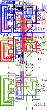
Figure 24: The merging gadget.

Interconnecting the gadgets.

Now, we describe how to interconnect the gadgets.

We place the sentence gadgets $G(s_{1}),\dots,G(s_{m})$ to the left of the merging gadget $M$ in a top-down ordering. Similarly, we place $G(\widehat{s}_{1}),\dots,G(\widehat{s}_{m})$ to the right, again in a top-down ordering. First, for any $\bar{s}\in S\cup\widehat{S}$ and $i\in\{0,2,3,\dots,\ell(\bar{s})\}$ (that is, $i\neq 1$), we connect $\gamma_{i}(\bar{s})$ with the $(i+1)$th pair of loose ends of $M(\bar{s})$ by a pair of parallel arcs as directly as possible without introducing new crossings; see Figure 25.

Figure 25: The first step of interconnecting the gadgets: Connecting $M(s)$ to the arcs $\gamma_{i}(s)$ for $i\neq 1$. The mirror symmetric part for $\widehat{s}$ is not displayed.

Now we want to connect $\gamma_{1}(\bar{s})$ to the second pair of loose ends of $M(\bar{s})$. For simplicity, we describe this in the case $\bar{s}=s\in S$. The case $\bar{s}\in\widehat{S}$ is mirror symmetric. We pull a pair of parallel arcs from $\gamma_{1}(s)$ with the aim to reach $M(s)$ while obeying the following rules:

1. We are not allowed to cross the merging gadget or the sentence gadgets (except the case described in the third rule below). We keep the newly introduced arcs on the left side from the merging gadget.

2. We are allowed to cross other pairs of parallel arcs introduced previously (when connecting $\gamma_{i}(s^{\prime})$ to $M(s^{\prime})$ for some $i$ and $s^{\prime}$). However, if we cross such a pair, we require that all four newly introduced crossings are resolved simultaneously (for example the new pair of parallel arcs is always above the older one). We even allow a self crossing of the newly introduced parallel arcs (but we again require that four newly introduced crossings are resolved simultaneously).

3. For every relation $R=(T,s^{\prime})$ where $s\in T$, let $R=R_{i}(s^{\prime})$. We interlace the newly introduced parallel arcs with $\gamma_{i}(s^{\prime})$ as in Figure 26. For further reference, two important crossings are denoted $z^{1}_{i}(s^{\prime},s)$ and $z^{2}_{i}(s^{\prime},s)$ as in the figure.

4. The total number of crossing is of polynomial size in the size of our instance $(S,\mathcal{R})$.

Figure 26: Interlacing the parallel arcs pulled out of $\gamma_{1}(s)$ with $\gamma_{j}(s^{\prime})$.

As we have quite some freedom how to perform the construction obeying the rules above, the resulting construction is not unique. An example how to get this construction systematically is sketched on Figure 27: The newly introduced pair of arcs is pulled little bit to the right, then we continue down towards the level of $G(s_{m})$, then up towards the level of $G(s_{1})$, and then back down to the original position. On this way we make a detour towards $\gamma_{j}(s^{\prime})$ whenever we need to apply the rule (R3). Finally, we connect the parallel arcs to $M(s)$ without any further detour.

Figure 27: The second step of interconnecting the gadgets: Connecting $M(s)$ to the arc $\gamma_{1}(s)$. The mirror symmetric part of $\widehat{s}$ is again not displayed. The arcs $\delta(s)$ are distinguished by colors.

For a later analysis, note that for any $s\in S$, the merging gadget $M(s)$, the sentence gadget $G(s)$ and the newly introduced pairs of parallel arcs connecting $\gamma_{i}(s)$ and $M(s)$ altogether form a single arc. We will denote this arc $\delta(s)$. In particular each arc $\gamma_{i}(s)$ is a subarc of $\delta(s)$. As usual, we also use the analogous notation for $\widehat{s}$.

Note that after all these steps, we obtain a diagram of a knot, which is our desired diagram—it is the union of arcs $\delta(\bar{s})$ for $\bar{s}\in S\cup\widehat{S}$. We denote this diagram $D(S,\mathcal{R})$. A little bit more of investigation reveals that $D(S,\mathcal{R})$ is actually a diagram of an unknot but we do not really need this.

6.3 A small set of axioms implies small defect

Let us assume that $D(S,\mathcal{R})$ is a diagram coming from a preprocessed instance $(S,\mathcal{R},k)$. The aim of this subsection is to show that if there exists a set $A$ of axioms of size $k$ for $(S,\mathcal{R})$, then there exists an untangling of $D(S,\mathcal{R})$ with defect $2k$. In other words, we will show that if $(S,\mathcal{R},k)$ is a (preprocessed) Yes instance of Minimum Axiom Set, then $(D(S,\mathcal{R}),2k)$ is a Yes instance of Unknotting via defect.

We will provide an untangling ${\mathcal{D}}$ that uses only $\rm{I}^{-}$ and $\rm{II}^{-}$ moves. By Lemma 3, the defect of ${\mathcal{D}}$ equals to the number of $\rm{I}^{-}$ moves.

We first describe the $\rm{I}^{-}$ moves. For every $a\in A$, we unscrew the loop next to $y(a)$ by a $\rm{I}^{-}$ move (see Figure 22 for $y(a)$) as well as we unscrew the loop next to $y(\widehat{a})$. For this, we need $2k$ $\rm{I}^{-}$ moves. It remains to show that the resulting diagram can be untangled using $\rm{II}^{-}$ moves only.

Next, we use $\rm{II}^{-}$ moves to untangle $\gamma_{0}(a)$ from the sentence gadget; see Figure 28. After this step, the only remainder of $\gamma_{0}(a)$ is a loop next to the other self-crossing of $\gamma_{0}(a)$.

Figure 28: $\rm{II}^{-}$ moves after unscrewing the loop at $y(a)$. Compare with Figures 22 and 26.

After untangling $\gamma_{0}(a)$, we may untangle $\gamma_{1}(a)$ from $G(a)$ using the $\rm{II}^{-}$ moves only; see Figure 29. First, we untangle $\gamma_{1}(a)$ form $\gamma_{2}(a)$ (if $\gamma_{2}(a)$ exists) as suggested in the left figure. (This can be done so that we first untangle the inner ‘finger’ and then the outer one.) Then we untangle the head of $\gamma_{1}(a)$ form the other $\delta(s)$ as suggested in the right figure. (Again we first untangle the inner finger, then the outer one.) Finally, we untangle the remainder all the way to $M(a)$. Due to our conventions (R1) and (R2) when interconnecting gadgets, it is possible to do this step via $\rm{II}^{-}$ moves.

Figure 29: $\rm{II}^{-}$ moves untangling $\gamma_{1}(a)$ from the gadget $G(a)$.

After untangling $\gamma_{1}(a)$ from $G(a)$, we may continue and untangle $\gamma_{2}(a)$ the same way, etc. until we untangle $\gamma_{\ell}(a)$. After these steps the only remainder from $\delta(a)$ is the merging gadget $M(a)$, a pair of parallel arcs towards the remainder of $\gamma_{0}(a)$, and this remainder of $\gamma_{0}(a)$ itself (a loop next to an original self-crossing of $\gamma_{0}(a)$).

Now, we repeatedly perform the following steps. Whenever $R=(T,s)$ is a relation in $\mathcal{R}$ such that each $t\in T$ is already almost untangled, then we want to untangle $s$ from the diagram. We recall that $R=R_{i}(s)$ for some $i\in\ell(s)$. Because each $t\in T$ is already almost untangled, the head of $\gamma_{i}(s)$ is now empty (it is obvious for axioms in $T$ but we will also keep the property that any newly almost untangled sentences leave all heads). This allows us to untangle $\gamma_{i}(s)$ from $G(s)$ in completely analogous way as we have untangled $\gamma_{0}(a)$ on Figure 28. Next, we can untangle $\gamma_{i+1}(s),\dots,\gamma_{\ell(s)}(s)$ using the same procedure as for $\gamma_{1}(a)$ on Figure 29. Using the same procedure again, we can also untangle $\gamma_{0}(s)$ with the exception that we stop at the two self crossings of $\gamma_{0}(s)$; then we remove these self-crossings by a $\rm{II}^{-}$ move, and then we continue all the way towards $M(s)$. After untangling $\gamma_{0}(s)$, we continue to $\gamma_{1}(s)$ and so on until we reach $\gamma_{i-1}(s)$. At this moment we say that $s$ is almost untangled from the diagram. (One could argue that $s$ is fully untangled at this moment because even the self-crossings of $\gamma_{0}(s)$ have been eliminated. But we want to use just one notion for well working recursion.)

We perform completely analogous steps for $\widehat{R}$ and $\widehat{s}$, getting $\widehat{s}$ untangled as well.

Because $A$ was a set of axioms, every sentence becomes almost untangled after finitely many steps. Now the diagram looks like as on Figure 30. The loop in position of $\gamma_{0}(s)$ and $\gamma_{0}(\widehat{s})$ appears if and only if $s\in A$. It is now easy to finish the untangling using $\rm{II}^{-}$ moves only. We untangle each $M(s)$ and $M(\widehat{s})$ one by one in top-down order. If $s$ is an axiom then the remaining self-crossing of $\gamma_{0}(s)$ cancels out with the self-crossing of $M(s)$, and the same is true for $\widehat{s}$. If $s$ is not an axiom, then the self crossings of $M(s)$ and $M(\widehat{s})$ cancel out together.

Figure 30: The diagram after untangling every sentence. In this figure $s_{1}\in A$ while $s_{2},s_{m}\not\in A$.

6.4 Big minimum axiom set implies big defect

Let us assume that $D(S,\mathcal{R})$ is a diagram coming from a preprocessed instance $(S,\mathcal{R},k)$. Our aim is to show that if the minimum axiom set for $(S,\mathcal{R})$ has size at least $k$, then any untangling of $D(S,\mathcal{R})$ has defect at least $2k$. This implies that if $(S,\mathcal{R},k-1)$ is a (preprocessed) No instance of Minimum Axiom Set, then $(D(S,\mathcal{R}),2(k-1))$ is a No instance of Unknotting via defect. (The shift of the parameter by $1$ appears only because of the convenience of the first formulation with which we will work.)

By Observation 16 our aim can be equivalently rephrased as follows: If the minimum axiom set for the double $(S\cup\widehat{S},\mathcal{R}\cup\widehat{\mathcal{R}})$ has size at least $2k$, then any untangling of $D(S,\mathcal{R})$ has defect at least $2k$.

One of the key tools will be the boosting lemma (Lemma 15) used for $(S\cup\widehat{S},\mathcal{R}\cup\widehat{\mathcal{R}})$. Given an untangling ${\mathcal{D}}$ of $D(S,\mathcal{R})$ we will design a function $\mu\colon S\cup\widehat{S}\to{\mathbb{Z}}$ satisfying the assumptions of the lemma such that $\operatorname{def}({\mathcal{D}})\geq\mu(S\cup\widehat{S})$; here we again extend the definition of $\mu$ to all subsets of $S\cup\widehat{S}$ as in the statement of the lemma. Then, by the lemma we deduce that $\operatorname{def}({\mathcal{D}})\geq 2k$ as we need.

Weights on crossings.

In order to define $\mu$ we will need to bound the defect via weights on crossings as in [dMRST21]. However, we need a little bit less, thus we will use a simpler weight function.

Let ${\mathcal{D}}$ be an untangling of a diagram $D$. Every crossing in $D$ has to be eventually removed by a $\rm{I}^{-}$ move or a $\rm{II}^{-}$ move during the untangling (of course, new crossings may appear but we are not interested in those for the moment). A $\rm{II}^{-}$ move in the untangling ${\mathcal{D}}$ is economical if it removes two crossings of $D$ whereas it is wasteful if at least on of the crossings removed by this $\rm{II}^{-}$ move was not originally in $D$ but it has been introduced during the untangling. We define the weight $w^{\prime}(x)$ of a crossing $x$ in $D$ by the following formula

$$w^{\prime}(x)=\begin{cases}0&\hbox{ if $x$ is removed by an economical $\rm{II}^{-}$ move,}\\ 1&\hbox{ if $x$ is removed by a $\rm{I}^{-}$ move,}\\ 2&\hbox{ if $x$ is removed by a wasteful $\rm{II}^{-}$ move.}\\ \end{cases}$$

The following lemma is a weaker form of Lemma 7 from [dMRST21].

Lemma 17.

Let ${\mathcal{D}}$ be an untangling of a diagram $D$. Then

$$\operatorname{def}({\mathcal{D}})\geq\sum_{x}w^{\prime}(x)$$

where the sum is over all crossings $x$ in $D$.

For completeness, we provide (almost complete) sketch of the lemma. For a slightly different full proof we refer to [dMRST21].

Sketch..

Using Lemma 3 it is sufficient to show that $\sum_{m}w(m)\geq\sum_{x}w^{\prime}(x)$ where the first sum is over all Reidemeister moves $m$ in ${\mathcal{D}}$. If $w^{\prime}(x)=1$, then $x$ is removed by a $\rm{I}^{-}$ move $m$, and thus we have $w(m)\geq w^{\prime}(x)$ for this $m$ and $x$. If $w^{\prime}(x)=2$, then $x$ is removed by a $\rm{II}^{-}$ move $m$ simultaneously with some $y$ which has been created during the untangling. This $y$ has been created either by a $\rm{I}^{+}$ move $m^{\prime}$ or a $\rm{II}^{+}$ move $m^{\prime\prime}$. Then we use $w(m^{\prime})\geq w^{\prime}(x)$ or $\frac{1}{2}w(m^{\prime\prime})\geq w^{\prime}(x)$. Summing all such inequalities, possibly with trivial inequalities $cw(m)\geq 0$ where $c\in\{1/2,1\}$ yields the desired result. ∎

Important crossings

Now we recall that our diagram $D(S,\mathcal{R})$ contains several important crossings, namely the crossings $x^{j}_{i}(\bar{s})$ for $\bar{s}\in S\cup\widehat{S}$, $i\in\{0,\dots,\ell(\bar{s})\}$ and $j\in[32]$; the crossings $y(\bar{s})$ for $\bar{s}\in S\cup\widehat{S}$ (see the definition of the sentence gadget and Figures 23 and 22 for the first two types); and the crossings $z^{1}_{i}(\bar{s},\bar{s}^{\prime}),z^{2}_{i}(\bar{s},\bar{s}^{\prime})$ for $\bar{s},\bar{s}^{\prime}\in S\cup\widehat{S}$ and $i\in\{0,\dots,\ell(\bar{s})\}$ such that $R_{i}(\bar{s})$ is of form $(T,\bar{s})$, where $\bar{s}^{\prime}\in T$ (see the rule (R3) when interconnecting the gadgets and Figure 26).

Now, for $\bar{s}\in S\cup\widehat{S}$ we set

$$X_{i}(\bar{s}):=\{x^{j}_{i}(\bar{s})\colon j\in[32]\} \hbox{ for }i\in\{0,\dots,\ell(s)\};$$

$$X(\bar{s}):=\bigcup_{i=0}^{\ell(\bar{s})}X_{i}(\bar{s});$$

$$Z_{i}(\bar{s}):=\{z_{i}^{j}(\bar{s},\bar{s}^{\prime})\colon j\in[2],R_{i}(\bar{s})=(T,\bar{s})\hbox{ with }\bar{s}^{\prime}\in T\} \hbox{ for }i\in[\ell(s)];$$

$$Z(\bar{s}):=\bigcup_{i=1}^{\ell(\bar{s})}Z_{i}(\bar{s});\hbox{ and}$$

$$Q(\bar{s}):=X(\bar{s})\cup\{y(\bar{s})\}\cup Z(\bar{s}).$$

Here $Q(\bar{s})$ is a set of important crossings assigned to $\bar{s}$. Note that if $\bar{s}\neq\bar{s}^{\prime}$, then $Q(\bar{s})$ and $Q(\bar{s}^{\prime})$ are disjoint.

Definition of $\mu$.

From now on let ${\mathcal{D}}$ be any untangling of $D(S,\mathcal{R})$. We define $\mu\colon S\cup\bar{S}\to{\mathbb{Z}}$ as

$$\mu(\bar{s}):=\sum_{x\in Q(\bar{s})}w^{\prime}(\bar{s})$$

where the weight $w^{\prime}$ corresponds to the untangling ${\mathcal{D}}$, of course. The function $\mu$ is nonnegative. In order to verify the assumptions of Lemma 15, we need to show the following.

Proposition 18.

Let $\bar{U}\subseteq S\cup\widehat{S}$ be such that $(S\cup\widehat{S})\setminus\bar{U}$ is not a set of axioms. Then $\mu(\bar{u})\geq 1$ for some $\bar{u}\in\bar{U}$.

Before we prove Proposition 18, let us explain how we finish our hardness proof (which we already sketched earlier). Assuming Proposition 18, we obtain $\mu(S\cup\widehat{S})\geq 2k$ by Lemma 15. On the other hand, as the sets $Q(\bar{s})$ are pairwise disjoint, we get that $\mu(S\cup\widehat{S})$ is at most the sum of the weights of all crossings in $D(S,\mathcal{R})$. Therefore $\operatorname{def}({\mathcal{D}})\geq\mu(S\cup\widehat{S})\geq 2k$ by Lemma 17. This is exactly what we need. Thus it remains to prove Propostion 18 which still requires a bit of effort.

Close neighbors.

For a proof of Proposition 18, we will need a notion of close neighbors from [dMRST21]. Let $Q$ be a set of crossings in a diagram $D$. Let $x$ and $y$ be two crossings of $D$, not necessarily in $Q$. We say that $x$ and $y$ are close neighbors with respect to $Q$ if $x$ and $y$ can be connected by two arcs $\alpha$ and $\beta$ satisfying the following conditions.

• $\alpha$ enters both $x$ and $y$ as an overpass;

• $\beta$ enters both $x$ and $y$ as an underpass;

• $\alpha$ and $\beta$ may have self-crossings; however neither $x$ nor $y$ is in the interior of $\alpha$ or $\beta$;

• no point of $Q$ is in the interior of $\alpha$ or $\beta$.

Let us remark that what we call close neighbors is a special case of $c$-close neighbors in [dMRST21] for $c=0$.

The following lemma is a special case of Lemma 9 in [dMRST21].

Lemma 19.

Let $Q$ be a set of crossings in a diagram $D$. Let us fix an untangling of $D$ and let $q$ be the first crossing in $Q$ removed by an economical $\rm{II}^{-}$ move (in this untangling). (In case of a tie, the conclusion is valid for both first two crossings.) Then there is a crossing $q^{\prime}$ in $D$ such that $q$ and $q^{\prime}$ are close neighbors with respect to $D$.

We again provide only a sketch while we refer to [dMRST21] for a full proof.

Sketch.

Because $q$ is removed by an economical $\rm{II}^{-}$ move, the second crossing removed by this $\rm{II}^{-}$ move also belongs to $D$. This is the desired $q^{\prime}$. At the moment of removal of $q$ and $q^{\prime}$, they from a ‘bigon’ along which the $\rm{II}^{-}$ move is performed. In particular they are connected by two arcs, one entering both as overpass and another one as underpass. Now we trace back the ‘history’ of the untangling up to this point and each step we ‘pull back’ this pair of arcs. By an analysis of the Reidemeister moves, it turns out that we will get $\alpha$ and $\beta$ required by the definition of close neighbors after returning to $D$ (while tracing back the history). ∎

Proof of Proposition 18..

We know that $(S\cup\widehat{S})\setminus\bar{U}$ is not a set of axioms for $(S\cup\widehat{S},\mathcal{R}\cup\widehat{\mathcal{R}})$. By the definition of the double of $(S,\mathcal{R})$, either $S\setminus\bar{U}$ is not a set of axioms for $(S,\mathcal{R})$, or $\widehat{S}\setminus\bar{U}$ is not a set of axioms for $(\widehat{S},\widehat{\mathcal{R}})$. Without loss of generality, we assume the former case, the argument for the latter case is symmetric. So we set $U:=\bar{U}\cap S$, and we assume that $S\setminus U=S\setminus\bar{U}$ is not a set of axioms. We will find $u\in U$ with $\mu(u)\geq 1$ as required.

First we perform the following simplification step. Assume that there is a relation $(T,s)\in\mathcal{R}$ such that $s\in U$ and $T\subseteq S\setminus U$. Let $U^{\prime}:=U\setminus\{s\}$. We observe that $S\setminus U^{\prime}$ is not a set of axioms. Indeed, $T\subseteq S\setminus U^{\prime}$ because we assume that $s\not\in T$ by the third step of preprocessing. This means that $s$ can be deduced from $S\setminus U^{\prime}$ which shows that the closures $c(S\setminus U)$ and $c(S\setminus U^{\prime})$ are equal. Thus $S\setminus U^{\prime}$ is not a set of axioms by an assumption that $S\setminus U$ is not a set of axioms. Thus, we can use $U^{\prime}$ instead of $U$ in our further considerations. Once we show that $\mu(u)\geq 1$ for some $u\in U^{\prime}$, then $u\in U$ as well. We repeat this simplification step as long as possible and we will perform our considerations for the resulting set. With a slight abuse of notation, we will still denote this set by $U$. In other words, we assume, without loss of generality, that if $(T,s)\in\mathcal{R}$ and $s\in U$, then $T\cap U\neq\emptyset$.

For contradiction, let us assume that $\mu(u)=0$ for every $u\in U$. This means that $w^{\prime}(x)=0$ for every $x\in Q$ where $Q:=\bigcup_{u\in U}Q(u)$. By the definition of $w^{\prime}$, this means that every $x\in Q$ is removed by an economical $\rm{II}^{-}$ move. Let $q$ be the first crossing in $I$ removed by an economical $\rm{II}^{-}$ move (in case of a tie, we take $q$ to be any of the first two removed crossings). By Lemma 19, there is a crossing $q^{\prime}$ of $D$ such that $q$ and $q^{\prime}$ are close neighbors with respect to $Q$.

Recall that $Q(u)=X(u)\cup\{y(u)\}\cup Z(u)$. We will distinguish between the cases whether $q\in X(u)$ for some $u$, or $q=y(u)$ for some $u$, or $q\in Z(u)$ for some $u$. In each case we will derive a contradiction with the fact that $q$ and $q^{\prime}$ are close neighbors.

Case 1: $q\in X(u)$ for some $u\in U$. As $q\in X(u)$ we get that $q\in X_{i}(u)$ for some $i\in\{0,\dots,\ell(u)\}$, that is, $q=x_{i}^{j}(u)$ for some $j\in[32]$. For each of the $32$ options, we seek for a possible $q^{\prime}$. A necessary condition, via the definition of close neighbors, is that $q$ and $q^{\prime}$ are connected by two arcs which do not contain any point of $Q$ in their interiors. In order to treat all $32$ options efficiently, we form a graph $G_{1}$ whose set of vertices is $Q$ and whose edges $xy$ where $x\in X_{i}(u)$ and $y\in Q$ correspond to arcs in $D$ which do not have any point of $Q$ in the interior; see Figure 31. We allow loops and multiple edges, therefore each $x\in X_{i}(u)$ has degree exactly $4$. An edge in the graph is drawn by a solid line if we guarantee that it corresponds to an arc which has no crossing in the interior. A dashed line is used if there may be some crossing (necessarily outside $Q$) in the interior of the corresponding arc. (In other words, we do not guarantee that this line is solid.) It is slightly non-trivial to check what are the other vertices of the edges emanating right from the points $x^{24}_{i}(u)$ and $x^{32}_{i}(u)$. This we will discuss in detail a bit later. All other edges depicted on Figure 31 follow immediately from the construction. (For the edges emanating down from $x^{31}_{i}(u)$ and $x^{32}_{i}(u)$ we do not make any claim on the figure.)

Figure 31: The graph $G_{1}$. In the figure, we write $x_{i}^{j}$ instead of $x_{i}^{j}(u)$. Compare with Figures 23 and 22 for $x$-labels and $y$-labels, and with Figure 26 for $z$-labels.

A necessary (but not sufficient) condition for $q$ and $q^{\prime}$ to be close neighbors is that $q\in X_{i}(u)$ and (i) either $q^{\prime}\in Q$ is connected to $q$ by at least two edges in $G_{1}$, or (ii) $q^{\prime}$ is a crossing of $D$ not in $Q$ and it belongs to at least two arcs corresponding to the edges in the graph. We will rule out both subcases but first let us analyze what are the neighbors of $x^{24}_{i}(u)$ and $x^{32}_{i}(u)$ on the right, as promised.

If $i=0$, then both $x^{24}_{i}(u)$ and $x^{32}_{i}(u)$ head to $y(u)$ without passing through any crossing. If $i\geq 1$, then we recall that $\gamma_{i}(u)$ corresponds to a relation $R_{i}(u)=(T,u)\in\mathcal{R}$. Let us also recall that the initial simplification of $U$ implies that $T\cap U\neq\emptyset$. Using the rule (R3) when interconnecting gadgets, this gives that the right neighbor of $x^{24}_{i}(u)$ is the rightmost $z_{i}^{1}(u,s)$ among all $s\in T\cap U$ and then the right neighbor of $x^{32}_{i}(u)$ is $z_{i}^{2}(u,s)$. In particular there is no double edge between $x^{24}_{i}(u)$ and $x^{32}_{i}(u)$.

Now, we rule out subcase (i), that is $q^{\prime}\in Q$ and $q$ and $q^{\prime}$ are connected by a double edge. We have double edges $x_{i}^{2}(u)x_{i}^{3}(u)$, $x_{i}^{6}(u)x_{i}^{7}(u)$, and possibly $x_{i}^{25}(u)x_{i+1}^{25}(u)$, if $\ell(u)=1$, that is, $i-1=i+1\pmod{\ell(u)+1}$. However, none of these cases yields close neighbors as the overpasses/underpasses disagree with the definition of close neighbors. (Compare with Figure 23 and with a modification of Figure 22 for $\ell=1$.) Seemingly, there could be also a double edge using $x^{32}_{i}(u)$ if the lower neighbor of $x^{32}_{i}(u)$ were $y(u)$ or $z^{2}_{i}(u,s)$. It is easy to rule out $y(u)$ as a lower neighbor of $x^{32}_{i}(u)$ by checking the arcs emanating from $y(u)$. For ruling out $z^{2}_{i}(u,s)$, we observe that an arc connecting $x^{32}_{i}(u)$ and $z^{2}_{i}(u,s)$ emanating down from $x^{32}_{i}(u)$ has to contain, for example, $x^{31}_{i}(u)$ before it may reach $z^{2}_{i}(u,s)$ (we simply pass through the diagram in this direction starting in $x^{32}_{i}(u)$ and check where we get). Thus $z^{2}_{i}(u,s)$ cannot be a lower neighbor of $x^{32}_{i}(u)$.

Next, we rule out subcase (ii), that is $q^{\prime}$ is not in $Q$ and it belongs to at least two arcs corresponding to the edges in the graph. By checking the dashed edges, the only option to get two such arcs is if $q=x^{32}_{i}(u)$. We rule out this case by a similar argument as before. Candidate $q^{\prime}$ to the right of $x^{32}_{i}(u)$ not in $Q$ may only be crossings intersecting the head of $\gamma_{i}(u)$ (recall that head is drawn on Figure 22). However, when trying to reach any such crossing from $x^{32}_{i}(u)$ by an arc emanating down, we have to meet $x^{31}_{i}(u)$ first again. This finishes the second subcase and therefore Case 1 of our analysis.

Case 2: $q=y(u)$ for some $u\in U$. This is almost trivial case: It is straightforward to check that $y(u)$ has no close neighbor $q^{\prime}$ (as the figure is only very local; see Figure 22).

Case 3: $q\in Z(u)$ for some $u\in U$. This means that $q=z_{i}^{j}(s,s^{\prime})$ for some $s,s^{\prime}\in S$ such that $R_{i}(s)=(T,s)$ with $s^{\prime}\in T$ and for some $j\in[2]$. We want to consider the subcases according to whether $q=z_{i}^{1}(s,s^{\prime})$ or $q=z_{i}^{2}(s,s^{\prime})$. For both case, we follow Figure 26 when describing the directions.

So, let us first assume that $q=z_{i}^{1}(s,s^{\prime})$. Because we need two arcs for close neighobors, we realize that the only candidates for $q^{\prime}$ are those that either intersect the head of $\gamma_{1}(s)$, or possibly $x^{32}_{i}(s)$ (the arc heading up is the only arc leaving the head among the arcs emanating from $z_{i}^{1}(s,s^{\prime})$). In addition, the arc emanating up heads towards $\gamma_{1}(s^{\prime})$ as requested by the construction; see Figure 26. In particular, it meets $x^{31}_{0}(s^{\prime})$ before it may meet any of the candidate $q^{\prime}$. Thus the arc emanating up from $z_{i}^{1}(s,s^{\prime})$ cannot be one of the witnesses that $q$ and $q^{\prime}$ are close neighbors. Therefore, the only crossing $q^{\prime}$ connected by two arcs to $z_{i}^{1}(s,s^{\prime})$ without points of $Q$ in their interiors may be $z_{i}^{2}(s,s^{\prime})$. But in this case, the overpasses/underpasses do not fit the definition.

Now, let us consider the case $q=z_{i}^{2}(s,s^{\prime})$. The reasoning is similar. The directions left, up and right reveal that any candidate close neighbor $q^{\prime}$ is in the head or it is the crossing $x^{31}_{i}(s)$. The bottom direction can be ruled out: It heads towards $M(s^{\prime})$ and then to $\gamma_{0}(s^{\prime})$. Before reaching the head of $\gamma_{1}(s)$ it thus has to reach $x^{32}_{\ell(s^{\prime})}(s^{\prime})$. Using the remaining directions, the only possible candidate is $q^{\prime}=z_{i}^{1}(s,s^{\prime})$. However, we have ruled out the pair $\{z_{i}^{1}(s,s^{\prime}),z_{i}^{2}(s,s^{\prime})\}$ as close neighbors already in the previous case.

This finishes the case analysis thereby the proof of Proposition 18 and the hardness part of Theorem 2. ∎

References

- [AGK+11] Noga Alon, Gregory Z. Gutin, Eun Jung Kim, Stefan Szeider, and Anders Yeo. Solving max-r-sat above a tight lower bound. Algorithmica, 61(3):638–655, 2011.
- [BLPS16] B. A. Burton, T. Lewiner, J. Paixão, and J. Spreer. Parameterized complexity of discrete Morse theory. ACM Trans. Math. Software, 42(1):Art. 6, 24, 2016.
- [BRS19] U. Bauer, A. Rathod, and J. Spreer. Parametrized complexity of expansion height. arXiv:1910.09228, 2019.
- [CFG+14] Robert Crowston, Michael R. Fellows, Gregory Z. Gutin, Mark Jones, Eun Jung Kim, Fran Rosamond, Imre Z. Ruzsa, Stéphan Thomassé, and Anders Yeo. Satisfying more than half of a system of linear equations over GF(2): A multivariate approach. J. Comput. Syst. Sci., 80(4):687–696, 2014.
- [CFK+15] M. Cygan, F. V. Fomin, Ł. Kowalik, D. Lokshtanov, D. Marx, Ma. Pilipczuk, Mi. Pilipczuk, and S. Saurabh. Parameterized algorithms. Springer, Cham, 2015.
- [CJM+13] Robert Crowston, Mark Jones, Gabriele Muciaccia, Geevarghese Philip, Ashutosh Rai, and Saket Saurabh. Polynomial kernels for lambda-extendible properties parameterized above the poljak-turzik bound. In Anil Seth and Nisheeth K. Vishnoi, editors, IARCS Annual Conference on Foundations of Software Technology and Theoretical Computer Science, FSTTCS 2013, December 12-14, 2013, Guwahati, India, volume 24 of LIPIcs, pages 43–54. Schloss Dagstuhl - Leibniz-Zentrum für Informatik, 2013.
- [dBCvKO08] M. de Berg, O. Cheong, M. van Kreveld, and M. Overmars. Computational Geometry: Algorithms and Applications. Springer, 2008.
- [DF13] R. G. Downey and M. R. Fellows. Fundamentals of Parameterized Complexity. Springer, 2013.
- [dMRST21] A. de Mesmay, Y. Rieck, E. Sedgwick, and M. Tancer. The unbearable hardness of unknotting. Adv. Math., 381:107648, 36, 2021.
- [FG06] J. Flum and M. Grohe. Parameterized complexity theory. Texts in Theoretical Computer Science. An EATCS Series. Springer-Verlag, Berlin, 2006.
- [FGL+20] Fedor V. Fomin, Petr A. Golovach, Daniel Lokshtanov, Fahad Panolan, Saket Saurabh, and Meirav Zehavi. Parameterization above a multiplicative guarantee. In Thomas Vidick, editor, 11th Innovations in Theoretical Computer Science Conference, ITCS 2020, January 12-14, 2020, Seattle, Washington, USA, volume 151 of LIPIcs, pages 39:1–39:13. Schloss Dagstuhl - Leibniz-Zentrum für Informatik, 2020.
- [GKLM11] Gregory Z. Gutin, Eun Jung Kim, Michael Lampis, and Valia Mitsou. Vertex cover problem parameterized above and below tight bounds. Theory Comput. Syst., 48(2):402–410, 2011.
- [GP16] Gregory Z. Gutin and Viresh Patel. Parameterized traveling salesman problem: Beating the average. SIAM J. Discret. Math., 30(1):220–238, 2016.
- [GvIMY12] Gregory Z. Gutin, Leo van Iersel, Matthias Mnich, and Anders Yeo. Every ternary permutation constraint satisfaction problem parameterized above average has a kernel with a quadratic number of variables. J. Comput. Syst. Sci., 78(1):151–163, 2012.
- [Hak61] W. Haken. Theorie der Normalflächen. Acta Math., 105:245–375, 1961.
- [HLP99] J. Hass, J. C. Lagarias, and N. Pippenger. The computational complexity of knot and link problems. J. ACM, 46(2):185–211, 1999.
- [KL12] L. H. Kauffman and S. Lambropoulou. Hard unknots and collapsing tangles. In Introductory lectures on knot theory, volume 46 of Ser. Knots Everything, pages 187–247. World Sci. Publ., Hackensack, NJ, 2012.
- [KT21] D. Koenig and A. Tsvietkova. NP–hard problems naturally arising in knot theory. Trans. Amer. Math. Soc. Ser. B, 8:420–441, 2021.
- [Kup14] G. Kuperberg. Knottedness is in , modulo GRH. Adv. Math., 256:493–506, 2014.
- [Lac15] M. Lackenby. A polynomial upper bound on Reidemeister moves. Ann. of Math. (2), 182(2):491–564, 2015.
- [Lac16] M. Lackenby. The efficient certification of knottedness and Thurston norm. arXiv:1604.00290, 2016.
- [Lac17] M. Lackenby. Elementary knot theory. In Lectures on geometry, Clay Lect. Notes, pages 29–64. Oxford Univ. Press, Oxford, 2017.
- [Lac21] M. Lackenby. Marc Lackenby announces a new unknot recognition algorithm that runs in quasi-polynomial time. https://www.maths.ox.ac.uk/node/38304, 2021.
- [MR99] Meena Mahajan and Venkatesh Raman. Parameterizing above guaranteed values: Maxsat and maxcut. J. Algorithms, 31(2):335–354, 1999.
- [MRS09] Meena Mahajan, Venkatesh Raman, and Somnath Sikdar. Parameterizing above or below guaranteed values. J. Comput. Syst. Sci., 75(2):137–153, 2009.
- [MT01] B. Mohar and C. Thomassen. Graphs on surfaces. The Johns Hopkins University Press, 2001.