Top quark effective couplings from top-pair tagged photoproduction in $pe^{-}$ collisions

Abstract

We present a detailed study, at the fast detector simulation level, of top-pair photoproduction in semileptonic mode at the LHeC and FCC-he future colliders. We work in full tree-level QED, not relying on the equivalent-photon approximation, taking into account the complete photoproduction kinematics. This allows us to define three photoproduction regions based on the angular acceptance range of the electron tagger. Those regions provide different degrees of sensitivity to top-quark effective couplings. We focus on the $t\overline{t}\gamma$ dipole couplings and the left-handed vector $tbW$ coupling for which we determine limits at both energies and in different photoproduction regions. We find that the LHeC and FCC-he will yield tight direct bounds on top dipole moments, greatly improving on current direct limits from hadron colliders, and direct limits on the $tbW$ coupling as restrictive as those expected from the HL-LHC. We also consider indirect limits from $b\to s\gamma$ branching ratio and $CP$ asymmetry, that are well known to be very sensitive probes of top electromagnetic dipole moments.

1 Introduction

Among the most important areas of research of future $pe^{-}$ colliders, such as the Large Hadron-electron Collider (LHeC) and the Future Circular Collider (FCC-he), is the study of the top quark effective couplings to the Higgs and the electroweak bosons [1]. Indeed, top quark effective couplings is a phenomenological research area of great interest [2]-[13]. Top-pair and single-top production at the LHeC are very good probes for charged-current (henceforth CC) $tbW$ and neutral-current (NC) $ttZ$ effective couplings [14],[15]. Also, anomalous magnetic and electric dipole moments of the top quark can be very well probed through top-pair photoproduction in electron-proton collisions [16]–[20].

In a previous preliminary study we obtained the dependence of the parton-level cross section for top-pair photoproduction on the top quark electromagnetic dipole moments, in the context of the Standard Model Effective Field Theory (SMEFT), and established limits on those moments. In this paper we extend that study by including in our Monte Carlo simulations parton showering and hadronization, and fast detector simulation, thus making them more realistic. This is reflected, in particular, in the study of background processes with a variable number of jets. Even more important, however, is the fact that in [16] the cross sections for photoproduction were computed in the equivalent photon approximation (EPA), whereas in this paper we work in full tree-level QED, taking into account the complete kinematics of the photoproduction process. This extension leads to three important improvements with respect to [16]. First, it leads to a precise computation of cross sections, and of their dependence on the photoproduction kinematic variables such as the scattered-electron transverse momentum. It is well known that the EPA is valid in the logarithmic approximation and only near the reaction threshold (see section 6.8 and appendix E of [21]); we remove those limitations by working in full QED. Second, by taking account of the complete kinematics of the process we determine the phase-space region where there is sensitivity to the top dipole moments, and the complementary region where there is not. Third, we consider besides the electromagnetic (e.m.) dipole moments, also the left-handed vector $tbW$ coupling. We notice that in the EPA the cross-section dependence on that coupling can occur only through the top decay vertex, leading to very poor sensitivity. Here, the full QED computation uncovers a phase-space region where there is significant sensitivity to that effective coupling.

In [16] the top dipole moments were expressed in terms of the Wilson coefficient $C_{uB}^{33}\rule{0.0pt}{12.0pt}$ associated with the dimension-six effective operator $Q_{uB}^{33}$. Specifically, it was found in [16] that either the real part of the coefficient $C^{33}_{uBr}$ at values greater than $0.3$ or the imaginary part $C_{tBi}$ at values greater than $0.8$ would produce a measurable $18\%$ deviation from the Standard Model (SM) cross section. Sometime before [16] was published, we presented limits on $C^{33}_{uB}$ based on the cross-section measurement of $t{\overline{t}}\gamma$ production at CDF that were substantially weaker: $|C^{33}_{uB}|<17.0$ (either real or imaginary part) [22]. In that same report we made an estimate of a then-future sensitivity of $t{\overline{t}}\gamma$ production at the LHC at energies of $7$ or $14$TeV, and our conclusion was that LHC should be able to set bounds of around $|C^{33}_{uB}|<3.0$ [22]. Recent studies, based on ATLAS measurements have indeed obtained limits of this size [23]. Also in [22] we obtained limits from $BR(B\to X_{s}\gamma)$ and $A_{CP}(B\to X_{s}\gamma)$ that were of similar size to the ones found from LHC data. Our analysis was based on a calculation of $\Delta C_{7}(m_{W})$, the variation of the SM $C^{\rm SM}_{7}(m_{W})$ due to new physics (NP) contributions from the magnetic and electric anomalous dipole moments of the top quark found in [24]. A recent study on dimension-six operators effects on $b\to s$ transitions has a new expression for $\Delta C_{7}(m_{W})$ that is very different and, in particular, predicts a much higher sensitivity of $BR(B\to X_{s}\gamma)$ [25]. To our knowledge there has been no disproof of either calculation. We shall, therefore, present updated limits from $BR(B\to X_{s}\gamma)$ and the associated $CP$ asymmetry based on the two possibilities.

The structure of this paper is as follows. In section 2 we discuss the effective Lagrangian framework of our study. We summarize there, also, the results of several recent global analyses of top quark effective couplings in that framework. In section 3 we carry out a Feynman-diagram analysis of the top-pair photoproduction process in $pe^{-}$ collisions in the SM. In section 4 we describe in detail the Monte Carlo simulations of the photoproduction process and its main irreducible background and obtain their cross sections in the SM. In section 5 we enumerate several additional SM background processes and assess their relative importance. In section 6 we present the limits to the top e.m. dipole moments and left-handed vector $tbW$ coupling at the LHeC and FCC-he energies in different photoproduction kinematical regions. In section 7 we give a summary of the paper and our final remarks. Several appendixes provide additional technical details on some issues discussed in the main text. Appendix A deals with our approach to neutrino momentum reconstruction. In appendix B we give the details on the calculation of effective-coupling limits from $BR(B\to X_{s}\gamma)$ and its associated asymmetry. In appendix C we restate some of the main results from section 6 in a different convention to facilitate comparison with other studies.

2 Effective SM Lagrangian

The framework we use in this paper is the SM effective Lagrangian with operators up to dimension six. In this context, the Lagrangian for top-pair photoproduction is of the form

$$\mathcal{L}=\mathcal{L}_{\mathrm{SM}}+\frac{1}{\Lambda^{2}}\sum_{\mathcal{O}}(\widehat{C}_{\mathcal{O}}\mathcal{O}+\mathrm{h.c.})+\cdots,$$ (1)

where $\mathcal{O}$ denotes dimension-six effective operators, $\Lambda$ is the new-physics scale, and the ellipsis refers to higher-dimensional operators. It is understood in (1) that the addition of the Hermitian conjugate, denoted $+\mathrm{h.c.}$ in the equation, is applicable only to non-Hermitian operators. Throughout this paper we use the dimension-six effective operators from the operator basis given in [26]. In particular, we use the same sign convention for covariant derivatives as in [16, 26], namely, $D_{\mu}=\partial_{\mu}+ieA_{\mu}$ for the electromagnetic coupling. However, we adopt the operator normalization defined in [27] (see also [28]), where a factor $y_{t}$ is attached to an operator for each Higgs field it contains, and a factor $g$ ($g^{\prime}$) for each $W_{\mu\nu}$ ($B_{\mu\nu}$) field-strength tensor. The Wilson coefficients in (1) are denoted $\widehat{C}$, since we will denote $C$ the coefficients associated with the original operator basis [26]. In fact, it will be convenient in what follows to express our results in terms of the modified dimensionless couplings

$$\widetilde{C}_{\mathcal{O}}=\widehat{C}_{\mathcal{O}}\frac{v^{2}}{\Lambda^{2}},$$ (2)

where $v$ is the Higgs-field vacuum expectation value. At tree level the coupling constants $\widetilde{C}_{\mathcal{O}}$ are independent of the scale $\Lambda$. We denote complex couplings as $\widetilde{C}_{\mathcal{O}}=\widetilde{C}_{\mathcal{O}\,r}+i\widetilde{C}_{\mathcal{O}\,i}$.

There are seven operators in the basis [26] that couple electroweak bosons and third family quarks. One of them is the focus of our study: $Q^{33}_{uB}$. Another one, $Q^{33}_{\varphi u}$, generates only a right-handed $ttZ$ coupling so that it will not contribute to the photoproduction process. Other four of them generate anomalous $tbW$ couplings: $Q^{33}_{\varphi ud}$, $Q^{33}_{uW}$, $Q^{33}_{dW}$ and $Q^{(3)33}_{\varphi q}$. The first three receive strong limits from top-decay $W$-helicity fractions [29, 30, 31] and, since the expected sensitivity of top-pair photoproduction to those couplings is low, we will not consider them further here. Unlike those three, $Q^{(3)33}_{\varphi q}$ only gets loose bounds from $W$-helicity fractions measurements. In a previous study we have obtained the LHeC sensitivity to the $tbW$ couplings from single-top production and indeed we have found that the HL-LHC would give stronger (individual) constraints on the tensorial $Q^{33}_{uW}$ and $Q^{33}_{dW}$ operators [14]. On the other hand, the LHeC would have better sensitivity than the HL-LHC for $Q^{(3)33}_{\varphi q}$ [14] (and to a lesser degree, also for $Q^{33}_{\varphi ud}$). To date, the strongest direct bounds to $Q^{(3)33}_{\varphi q}$ come from single-top production cross sections at the LHC [32]. Besides $Q^{33}_{uB}$, which is the focus of our study, we will also include the left-handed $tbW$ operator $Q^{(3)33}_{\varphi q}$ in our analysis because, as we show below, $t\overline{t}$ photoproduction at the LHeC and FCC-he can also be a competitive probe for this coupling. However, a redefinition of this operator that is also commonly used in the literature [33] will be necessary. $Q^{(3)33}_{\varphi q}$ and $Q^{(1)33}_{\varphi q}$ both generate $ttZ$ and $bbZ$ couplings. As the latter receives very strong constraints from bottom-quark production at the $Z$-pole (LEP and SLAC), we will have to combine the operators $Q^{(3)33}_{\varphi q}$ and $Q^{(1)33}_{\varphi q}$ so as to eliminate the $bbZ$ neutral current term [34, 35]. Thus, those operators will not be considered by themselves but rather in a particular linear combination.

In this paper we will, therefore, set up our analysis by focusing on just two operators: $\mathcal{O}_{uB}^{33}$ and $\mathcal{O}^{(-)33}_{\varphi q}$. Expanding these operators in physical fields yields, with the conventions discussed above:

$$\mathcal{O}^{33}_{uB} =y_{t}g^{\prime}Q^{33}_{uB}=\sqrt{2}y_{t}e(v+h)(\partial_{\mu}A_{\nu}-\tan\theta_{W}\partial_{\mu}Z_{\nu})\;\overline{t}_{L}\sigma^{\mu\nu}t_{R}~{},$$ (3)

$$\mathcal{O}_{\varphi q}^{(-)33} =\mathcal{O}_{\varphi q}^{(3)33}-\mathcal{O}_{\varphi q}^{(1)33}=-y_{t}^{2}Q_{\varphi q}^{(-)33}$$

$$=-y_{t}^{2}\frac{g}{\sqrt{2}}(v+h)^{2}\left(W^{+}_{\mu}\,\overline{t}_{L}\gamma^{\mu}b_{L}+W^{-}_{\mu}\,\overline{b}_{L}\gamma^{\mu}t_{L}\right)-y_{t}^{2}\frac{g}{c_{W}}(v+h)^{2}Z_{\mu}\,\overline{t}_{L}\gamma^{\mu}t_{L}\,,$$

where $Q^{33}_{uB}$, $Q_{\varphi q}^{(-)33}$ are the operators defined in [26]. Notice that both operators $\mathcal{O}^{33}_{uB}$ and $\mathcal{O}_{\varphi q}^{(-)33}$ are $O(g^{1})$ with respect to the weak coupling constant, which makes the definitions (3) consistent from the point of view of perturbation theory. We stress here the definition $\mathcal{O}_{\varphi q}^{(-)33}=\mathcal{O}_{\varphi q}^{(3)33}-\mathcal{O}_{\varphi q}^{(1)33}$ we use, since sometimes in the literature the opposite sign is used. The effective Lagrangian used throughout this paper results from substituting (3) and (2) in the Lagrangian (1). It is convenient to record here the relation between the Wilson coefficients in the form (2) and those associated with the original basis [26] (see also [36]). From the relation

$$\mathcal{L}=\mathcal{L}_{\mathrm{SM}}+\frac{1}{\Lambda^{2}}\sum_{\mathcal{Q}}(C_{Q}Q+\mathrm{h.c.})+\cdots,$$

analogous to (1), we obtain

$$C_{uB}^{33}=\frac{\Lambda^{2}}{v^{2}}y_{t}g^{\prime}\widetilde{C}_{uB}^{33}\rule{0.0pt}{12.0pt}=5.906\widetilde{C}_{uB}^{33}\rule{0.0pt}{12.0pt}~{},\qquad C_{\varphi q}^{(-)33}=-\frac{\Lambda^{2}}{v^{2}}y_{t}^{2}\widetilde{C}_{\varphi q}^{(-)33}\rule{0.0pt}{12.0pt}=-16.495\widetilde{C}_{\varphi q}^{(-)33}\rule{0.0pt}{12.0pt}~{}.$$ (4)

The numerical values in this equation arise from the parameters $\Lambda=1$ TeV, $v=246$ GeV, $g^{\prime}=0.358$, $g=0.648$. Furthermore, for all practical purposes we set $y_{t}=1=V_{tb}$. We point out here that the couplings $\widetilde{C}_{\varphi q}^{(-)33}\rule{0.0pt}{12.0pt}$, $\widetilde{C}_{uB}^{33}\rule{0.0pt}{12.0pt}$ are both of $O(g^{0})$ in the perturbative expansion and, therefore, from (4) $C_{\varphi q}^{(-)33}$ is $O(g^{0})$ but $C_{uB}^{33}$ is $O(g^{1})$.

It is common practice in the literature to write the anomalous interactions in terms of form factors. We adopt here the definition of top electromagnetic dipole moments given in eq. (2) of [16], and the CC vertex form factors from eq. (7.1) of [32],

$$\mathcal{L}_{\mathrm{anom}} =\mathcal{L}_{\mathrm{anom,em}}+\mathcal{L}_{\mathrm{anom,CC}}~{},$$ (5)

$$\mathcal{L}_{\mathrm{anom,em}} =\frac{e}{4m_{t}}\overline{t}\,\sigma^{\mu\nu}(\kappa+i\widetilde{\kappa}\gamma_{5})\,t\;F_{\mu\nu}~{},$$

$$\mathcal{L}_{\mathrm{anom,CC}} =\frac{g}{\sqrt{2}}f_{V}^{L}\left(W^{+}_{\mu}(\overline{t}_{L}\gamma^{\mu}b_{L})+W^{-}_{\mu}(\overline{b}_{L}\gamma^{\mu}t_{L})\right)~{},\quad f_{V}^{L}=V_{tb}+\delta f_{V}^{L}~{}.$$

Direct comparison of (5) with (1), (2), (3), yields the tree-level relations,

$$\kappa=2y_{t}^{2}\widetilde{C}_{uB\,r}^{33},\qquad\widetilde{\kappa}=2y_{t}^{2}\widetilde{C}_{uB\,i}^{33},\qquad\delta f_{V}^{L}=y_{t}^{2}\widetilde{C}_{\varphi q}^{(-)33}~{}.$$ (6)

The sign chosen in the last equality in (6) deserves clarification. Because the signs in the corresponding operator definitions (3) and (5) are opposite, a relative “$-$” sign could be expected in the relation between $\delta f_{V}^{L}$ and $\widetilde{C}_{\varphi q}^{(-)33}$. However, we define the SM CC Lagrangian in this paper with the same sign convention as in (3), and we assume that the analogous convention is made in [32], with the result that the interference term between the effective CC interaction and the SM one has the same sign (“$+$”) in both cases. Thus, (6) gives the correct relationship between $\delta f_{V}^{L}$ and $\widetilde{C}_{\varphi q}^{(-)33}$. We also notice here, that the particularly simple relations (6) are a consequence of eq. (2) and the operator normalization discussed above in the paragraph under eq. (1).

2.1 Overview of global analyses on top quark effective couplings.

In the last few years several research groups have reported extensive analyses of limits on certain sets of SMEFT dimension-six operators based, in turn, on certain sets of experimental observables. It is well known that no one experimental observable is only related to only one effective operator in isolation. Rather, for any observable there are usually four, five or many more independent operators that contribute. So the goal is not necessarily to prove that a certain observable is the best candidate to test one coupling in particular, but that this observable can contribute significantly to the pool of measurements that will be used in future ever more extensive analyses.

In a recent study constraints on the three top dipole operators $Q_{tB}$, $Q_{tW}$ and $Q_{tG}$ are obtained by using as experimental inputs the branching ratio $BR({\overline{B}}\to X_{s}\gamma)$ and two fiducial cross-section results of $t{\overline{t}}\gamma$ production by ATLAS [23]. It is found that, despite the large difference in sensitivities between $t{\overline{t}}\gamma$ and ${\overline{B}}\to X_{s}\gamma$ the inclusion of the less sensitive $t{\overline{t}}\gamma$ input still improves significantly the combined marginalized constraints. As far as experimental inputs the $BR({\overline{B}}\to X_{s}\gamma)$ stands out as probably the one observable that is most sensitive to the magnetic dipole operator $Q_{tB}$. However, we must also be aware of the fact that this is an indirect observable that is actually sensitive to most of the dimension-six operators with quark fields of the Warsaw basis [25]. And even so, $Q_{tB}$ is among those operators whose contribution to the Wilson coefficients of the effective Hamiltonian is not at the tree but at the one-loop level [25]. It is well known that direct observables, like production cross sections, their kinematic distributions and other related observables measured by colliders like the Tevatron and the LHC will always play the essential part of effective coupling studies.

Let us consider the reports of the last two years on global fits to gauge and Higgs boson combined with top and bottom quarks in the literature. In table 1 we show some of the limits reported by five collaborations: SMEFiT [33], TopFitter [37], Fitmaker [38], HEPfit [39] and EFTfitter [40]. Out of these five groups only the last one uses $B$ meson observables, while the rest rely mostly on ATLAS and CMS data on single top, $t\overline{t}$, $W$-helicity in top decay, and similar measurements of top quark processes. It is interesting to observe the very diverse scenarios they depict for individual constraints, as for instance Fitmaker and HEPfit obtain very stringent bounds on $C^{(3)}_{\varphi Q}$ as compared to SMEFiT and TopFitter, but then the exact opposite is true for $C_{tW}$ again among these four collaborations. On the other hand, once the global fit is performed and marginalized limits are obtained we do see a more uniform scenario, as is shown in the lower part of table 1. Since we are interested in the electromagnetic dipole coupling, we added the tag $t{\overline{t}}\gamma$ to the last three groups that used this LHC process in their fits, and then see if they would be the ones with better constraints on $C_{tB}$. Apparently, this is not quite the case, TopFitter and Fitmaker end up with similar limits despite one not relying on $t{\overline{t}}\gamma$. Of course, the best bounds (which are not even individual) appear in the last column; but we know that their strong bound really comes from $\overline{B}\to X_{s}\gamma$. We point out that the limits shown in Table 1 have been obtained using linear (or interference) contributions as well as quadratic (or purely anomalous) contributions to the chosen observables. These bounds are usually somewhat more stringent than the ones obtained with only linear terms. The exception is in the middle column, where the limits provided by Fitmaker [38] are only with linear terms.

$C$	SMEFiT [33]	TopFitter [37]	Fitmaker [38]	HEPfit [39]	EFTfitter [40]
			$t{\overline{t}}\gamma$	$t{\overline{t}}\gamma$	$t{\overline{t}}\gamma$,B
	individual 90% - 95% C.L.
$C^{(1)}_{\varphi Q}$	$--$	$-3.0\;,\;+0.8$	$-0.03\;,\;+0.05$	$--$	$--$
$C^{(3)}_{\varphi Q}$	$-0.38\;,\;+0.34$	$-0.3\;,\;+0.9$	$-0.03\;,\;+0.05$	$-0.02\;,\;+0.04$	$--$
$C^{(-)}_{\varphi Q}$	$-1.1\;,\;+1.6$	$--$	$--$	$-0.04\;,\;+0.08$	$--$
$C_{\varphi t}$	$-3.0\;,\;+2.2$	$-1.0\;,\;+4.5$	$-1.2\;,\;+2.9$	$-8.6\;,\;+1.5$	$--$
$C_{\varphi tb}$	$--$	$-0.3\;,\;+0.3$	$--$	$-6.6\;,\;+6.7$	$--$
$C_{tW}$	$-0.08\;,\;+0.03$	$-0.09\;,\;+0.09$	$-0.12\;,\;+0.51$	$-0.28\;,\;+0.32$	$--$
$C_{bW}$	$--$	$-0.05\;,\;+0.05$	$--$	$-0.47\;,\;+0.47$	$--$
$C_{tZ}$	$-0.04\;,\;+0.09$	$--$	$--$	$-0.39\;,\;+0.57$	$--$
$C_{tB}$	$--$	$-4.2\;,\;+4.5$	$-4.5\;,\;+1.2$	$--$	$--$
	marginalized 90% - 95% C.L.
$C^{(1)}_{\varphi Q}$	$--$	$--$	$-0.59\;,\;+0.58$	$--$	$\pm 0.43$
$C^{(3)}_{\varphi Q}$	$-0.62\;,\;+0.48$	$--$	$-0.67\;,\;+0.46$	$-1.29\;,\;+0.81$	$\pm 0.40$
$C^{(-)}_{\varphi Q}$	$-2.25\;,\;+2.86$	$--$	$--$	$-2.42\;,\;+2.29$	$--$
$C_{\varphi t}$	$-13.36\;,\;+3.96$	$--$	$+2\;,\;+11$	$-10.58\;,\;+1.12$	$\pm 13.2$
$C_{\varphi tb}$	$--$	$--$	$--$	$-7.6\;,\;+7.6$	$--$
$C_{tW}$	$-0.24\;,\;+0.09$	$--$	$-0.09\;,\;+0.55$	$-0.19\;,\;+0.50$	$\pm 0.50$
$C_{bW}$	$--$	$--$	$--$	$-0.98\;,\;+0.94$	$--$
$C_{tZ}$	$-1.13\;,\;+0.86$	$--$	$--$	$-0.37\;,\;+0.88$	$--$
$C_{tB}$	$--$	$--$	$-5.2\;,\;+2.5$	$--$	$\pm 0.58$

Table 1: Limits on the effective couplings at 90-95% C.L. from global fits reported in the last two years. Coefficients as defined in [26], and $C^{(1,3)}_{\varphi Q}=C^{(1,3)33}_{\varphi q}$, $C^{(-)}_{\varphi Q}=C^{(1)33}_{\varphi q}-C^{(3)33}_{\varphi q}$, $C_{tB}=C^{33}_{uB}$, $C_{tW}=C^{33}_{uW}$, $C_{tB}=C^{33}_{uB}$, $C_{tZ}=c_{w}C^{33}_{uW}-s_{w}C^{33}_{uB}$.

Concerning future projections for the limits of $C^{33}_{uB}$, or $\kappa$, $e^{+}e^{-}$ colliders like CLIC and ILC offer the highest sensitivity with potential bounds of order $|\kappa|\leq 0.003$ ($|C_{uB}^{33}|\leq 0.009$) and $|\kappa|\leq 0.002$ ($|C_{uB}^{33}|\leq 0.006$), respectively [41]. For the HL-LHC $tt\gamma$ a preliminary study in [42] (see also [43]) obtained $|\kappa|\leq 0.12$ ($|C_{uB}^{33}|\leq 0.36$) for $3{\rm ab}^{-1}$ luminosity. Recently, a more realistic analysis by [44] obtained a similar sensitivity for $3{\rm ab}^{-1}$ luminosity, with $-0.5\leq C_{uB}^{33}\leq 0.3$. These HL-LHC potential limits are similar to the bounds obtained here for LHeC, and also of similar size as the current $68\%$ C.L. individual bound from ${\overline{B}}\to X_{s}\gamma$ as shown in Appendix B.

3 Top-pair photoproduction in the SM: diagrammatic analysis

Figure 1: Unitary-gauge Feynman diagrams for the photoproduction of a top pair in semileptonic mode, see eq. (7). All diagrams for the final state $e^{-}\,b\ell^{+}\nu_{\ell}\,\overline{b}\overline{q}_{u}q_{d}$ are shown. Diagrams (c)–(i) are necessary to preserve electromagnetic gauge invariance when $t$, $W$ are off shell.

We are interested in this paper in top-pair photoproduction in $pe^{-}$ collisions in the semileptonic decay channel which, at parton level, leads to the seven-fermion final states,

$$g\;e^{-}\rightarrow e^{-}t\overline{t}\rightarrow e^{-}\,b\ell^{+}\nu_{\ell}\,\overline{b}\overline{q}_{u}q_{d}+e^{-}\,bq_{u}\overline{q}_{d}\,\overline{b}\ell^{-}\overline{\nu}_{\ell},\quad\mathrm{with}\;q_{u}=u,c,\;q_{d}=d,s,\;\ell=e,\mu.$$ (7)

This equation defines our signal process. The set of Feynman diagrams for this process in the photoproduction region in unitary gauge in the SM with Cabibbo mixing is shown in figure 1. For each possible final-state lepton ($\ell=e^{\pm}$, $\mu^{\pm}$) in (7) there are four possible quark-flavor combinations, and for each possible lepton and quark flavor combination there are nine diagrams in figure 1, except for $\ell=e^{-}$ for which the number of diagrams doubles, leading to a total of 180 Feynman diagrams for this process. We consider the top-pair photoproduction process defined by the diagrams in figure 1 our signal process, and denote its cross section by $\sigma_{\mathrm{sgnl}}$.

We can divide the set of diagrams in figure 1 into two subsets: the first subset includes diagrams (a), (b), containing three internal top lines, and the second one comprises the remaining diagrams, (c)–(i), containing two internal top lines. The second subset is necessary to preserve electromagnetic gauge invariance in the phase-space regions where $t$ or $W$ lines are off shell. There is, in fact, strong destructive interference between the two subsets in the photoproduction region, such that the total cross section $\sigma_{\mathrm{sgnl}}$ computed with all the diagrams is smaller than the cross sections obtained from (a), (b) or (c)–(i) separately, by a factor 10–25 depending on the cuts used in the computation.

Figure 2: Unitary-gauge Feynman diagrams for the associate photoproduction and decay of $tbW$ in semileptonic mode with leptonic top decay, see eq. (8). All diagrams for the final state $e^{-}\,b\ell^{+}\nu_{\ell}\,\overline{b}\overline{q}_{u}q_{d}$ corresponding to leptonic top decay are shown. Diagrams (e)–(i) are necessary to preserve electromagnetic gauge invariance when $t$, $W$ are off shell.

We must consider also other processes with the same final state as (7), which constitute irreducible backgrounds. Particularly important is the associate $tbW$ photoproduction, in which $bW$ does not originate in a top decay. For this process, in semileptonic mode, we have to distinguish the cases of leptonic and hadronic top decays,

$$ge^{-} \rightarrow e^{-}t\overline{b}W^{-}+e^{-}\overline{t}bW^{+}\rightarrow e^{-}\,b\ell^{+}\nu_{\ell}\,\overline{b}\overline{q}_{u}q_{d}+e^{-}\,\overline{b}\ell^{-}\overline{\nu}_{\ell}\,bq_{u}\overline{q}_{d},$$ (8)

$$ge^{-} \rightarrow e^{-}t\overline{b}W^{-}+e^{-}\overline{t}bW^{+}\rightarrow e^{-}\,bq_{u}\overline{q}_{d}\,\overline{b}\ell^{-}\overline{\nu}_{\ell}+e^{-}\,\overline{b}\overline{q}_{u}q_{d}\,b\ell^{+}\nu_{\ell},$$

with $q_{u}$, $q_{d}$, $\ell$ as in (7). These two sets of processes lead to the same final states, and to two different but completely analogous sets of Feynman diagrams. In figure 2 we show the corresponding diagrams for $t\overline{b}W^{-}$ photoproduction with leptonic $t$ decay. Taking into account the possible lepton and quark flavor channels, the duplication of diagrams for $\ell=e^{-}$, and the two types of processes in (8), we are led to a total of 360 Feynman diagrams for (8). There is strong destructive interference in the photoproduction region, similar to that described above for the signal process, between the subset of diagrams from figure 2 formed by diagrams (a)–(d) and that formed by (e)–(i). The latter is needed to preserve electromagnetic gauge invariance when $t$ or $W$ are off shell. This process, as discussed in detail below, is the main irreducible background to the signal process (7) and we denote its cross section by $\sigma_{tbW}$.

Figure 3: Unitary-gauge Feynman diagrams for the associate photoproduction and decay of $tbqq$ in leptonic mode, see eq. (9). All diagrams for the final state $e^{-}\,b\ell^{+}\nu_{\ell}\,\overline{b}\overline{q}_{u}q_{d}$ are shown. Diagrams (g)–(i) are necessary to preserve electromagnetic gauge invariance when $t$, $W$ are off shell.

Another process with the same final state as (7) that we must take into account is $tbqq$ photoproduction with leptonic top decay, in which the $qq$ does not arise from a $W$ decay,

$$ge^{-}\rightarrow e^{-}t\overline{b}\overline{q}_{u}q_{d}+e^{-}\overline{t}bq_{u}\overline{q}_{d}\rightarrow e^{-}\,b\ell^{+}\nu_{\ell}\,\overline{b}\overline{q}_{u}q_{d}+e^{-}\,\overline{b}\ell^{-}\overline{\nu}_{\ell}\,bq_{u}\overline{q}_{d},$$ (9)

with $q_{u}$, $q_{d}$, $\ell$ as in (7). In figure 3 we show the Feynman diagrams for the process (9) in its $t\overline{b}\overline{q}_{u}q_{d}$ form, containing a $gq_{d}\overline{q}_{d}$ vertex. From those diagrams, by exchanging $q_{d}\leftrightarrow\overline{q}_{u}$, $\overline{q}_{d}\leftrightarrow q_{u}$, another set of valid ones with a $gq_{u}\overline{q}_{u}$ vertex can be obtained, which is not shown for brevity. Taking account of the quark- and lepton- flavor multiplicity as above, and the diagrams with $gq_{u}\overline{q}_{u}$ vertex not shown, results in a total of 360 diagrams for process (9). As discussed below, $tbqq$ constitutes a small background to $t\overline{t}$ photoproduction that can be neglected.

We stress here that the diagrams for processes (7), (8), (9) exhaust all possible Feynman diagrams (900 in total) with the same initial and final states as those processes and with at least one internal top line, in the photoproduction region, in unitary gauge, in the SM with Cabibbo mixing. Furthermore, the interference between those processes is small, at the level of a few percent, so that it makes sense to consider $t\overline{t}$ photoproduction the signal process with $tbW$ and $tbqq$ as backgrounds.

4 Top-pair photoproduction in the SM: Monte Carlo simulations

We compute the tree-level cross section for top-pair photoproduction and its backgrounds with the matrix-element Monte Carlo generator MadGraph5_aMC@NLO (henceforth MG5) version 2.6.3 [45]. We use the parton distribution function (PDF) CTEQ6l as implemented in MG5. The cuts we apply at the parton level in MG5 are similar to those described below in connection with event selection, but substantially looser, in order to adequately populate phase space without inappropriately restricting it. As should be clear from the discussion in section 3, all resonant and non-resonant Feynman diagrams for this process are taken into account, as well as all off-shell and interference effects. In particular, the small-width approximation is not used in our simulations. We run Pythia version 6.428 [46] with MG5 events as initial data, with default parameters, for QCD/QED showering, hadronization and resonance decay. In the parton-level MG5 simulation we work in the four light flavors scheme, retaining the masses of the first two particle generations to keep Pythia’s event rejection rate at 0. We neglect, however, the Higgs boson couplings to the first two generations for numerical efficiency, since the light-mass effects are negligibly small.

We run Delphes version 3.4.2 [47] on Pythia events for fast detector simulation. Jet clustering is carried out in Delphes by means of FastJet 3.3.2 [48]. We carry out the analysis of Delphes events with Root version 6.22 [49]. For the LHeC and FCC-he detector simulations we use the configuration files developed by the experimental collaborations and distributed with Delphes as delphes_card_LHeC.tcl and delphes_card_FCCeh.tcl, respectively. In both cases we use default parameters, with the following exceptions. For jet clustering we use the anti-$k_{t}$ algorithm with default radius parameter 0.4, but we set JetPTMin to 10 GeV since we will have to introduce a cut on jet $p_{T}$ with $p_{T\,\mathrm{min}}\geq 10$ GeV to control irreducible backgrounds. Furthermore, we find that at the LHeC the cross section for top-pair photoproduction is somewhat small, and that reducible backgrounds are much less important than irreducible ones. We are thus led to choose a $b$-tagging algorithm with higher efficiency and lower purity than the default. We therefore change the settings in the LHeC configuration file from the default with $b$-tagging efficiency $\eta_{b}=0.75$, and $c$- and light-jet mistagging probabilities $p_{c}=0.05$ and $p_{j}=0.001$, respectively, to a working point with $\eta_{b}=0.85$, $p_{c}=0.1$, $p_{j}=0.01$. In the case of the FCC-he configuration file, we leave the default $b$-tagging working point unchanged which, for $|y|<2.5$, $5<p_{T}<400$ GeV, is given by $\eta_{b}=0.85$, $p_{c}=0.04$, $p_{j}=0.001$.

We assume that the scattered electron in the photoproduction process is detected either in the main detector, or in an appropriate forward one. We consider three rapidity intervals in which the scattered electron can be detected, thus determining three photoproduction regions. First, we assume that the main detector covers the range 1^∘–179^∘ (see section 11 of [50]), corresponding to $y=-4.741$ in the backward hemisphere. In fact, from tables 12.4 and 12.6 of [50] we see that both the tracker and electromagnetic calorimeter are expected to extend up to $\eta=-4.8$, so in this photoproduction region the scattered electron’s energy-momentum are measurable. Second, we assume that the scattered electron may be identified by a detector similar to the ones used for Compton scattering and luminosity measurements, with angular acceptance in the range 179^∘–179.5^∘, corresponding to $-5.435<y<-4.741$. Third, we assume that a small-angle electron tagger (see [50], section 13.1.4) covers the range $\pi-4$ mrad $<\theta(e^{-})<\pi-8.727$ mrad, or $-6.215<y(e^{-})<-5.435$. In summary, we define the three photoproduction regions,

$$PhP_{I}: \quad-4.741<y(e^{-})<-3.0,$$ (10)

$$PhP_{II}: \quad-5.435<y(e^{-})<-3.0,$$

$$PhP_{III}: \quad-6.215<y(e^{-})<-3.0.$$

For simplicity, we assume there are no gaps in each range. Notice that each region in (10) is defined to be contained by the following one. In fact, the upper limit of the rapidity interval is not very important in regions $PhP_{II}$ and $PhP_{III}$, as the dominant contribution to the SM photoproduction cross section originates in the lower part of the rapidity range, as illustrated in figure 4 (see left panel).

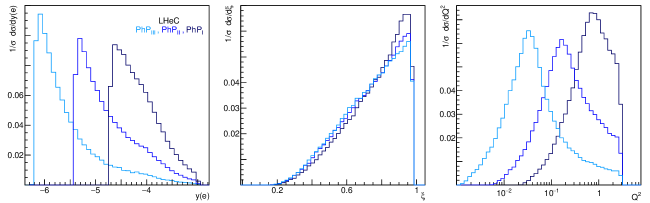
Figure 4: Normalized differential cross sections, with cuts $C_{0,\ldots,3}$, with respect to lab-frame scattered-electron rapidity (left panel), photon energy fraction (center) and photon squared virtuality (right). The three photoproduction regions (10) are illustrated, as indicated by the color code.

In order to determine the event kinematics we must first reconstruct the neutrino momentum. For processes such as $t\overline{t}$ and $tbW$ production in semileptonic mode, the transverse neutrino momentum is identified with the missing transverse momentum, and its longitudinal component is approximately reconstructed from $W$-decay kinematics. In appendix A we discuss in some detail our approach to neutrino-momentum reconstruction in asymmetric colliders such as the LHeC and FCC-he. We identify the two $b$-tagged jets with the highest $p_{T}$ as the ones originating in top decays, and denote them $J_{b\,0,1}$. The remaining $b$-tagged jets, if any, are treated as light jets. The set of light jets is ordered by decreasing $p_{T}$, and denoted $J_{k}$, $k=0,\ldots,N_{l}-1$. We identify the highest $p_{T}$ lepton, electron or muon, as the one arising from leptonic top decay. With this information, we divide the light jets into three subsets: jets arising from the hadronic top decay, $J_{\mathrm{hdr}\,k}$, $k=0,\ldots,N_{t\mathrm{hdr}}-1$, jets from the leptonic top decay, $J_{\mathrm{lpt}\,k}$, $k=0,\ldots,N_{t\mathrm{lpt}}-1$, and jets not arising from top decay, or “spectator” jets, $J_{\mathrm{spct}\,k}$, $k=0,\ldots,N_{\mathrm{spct}}-1$. Thus, the total number of jets in the event is $N_{J}=N_{b}+N_{t\textrm{hdr}}+N_{t\textrm{lpt}}+N_{\textrm{spct}}$. Each set of jets is ordered by decreasing $p_{T}$. We introduce the $\chi^{2}$ function

$$\chi^{2}=\frac{1}{\Gamma_{t}^{2}}\left(\left(m_{b_{0}\ell\nu j_{\mathrm{lpt}}}-m_{t}\right)^{2}+\left(m_{b_{1}j_{\mathrm{hdr}}}-m_{t}\right)^{2}\right),$$ (11)

where $m_{b_{0}\ell\nu j_{\mathrm{lpt}}}$ is the invariant mass of one of the two $b$-jets, together with the charged lepton and neutrino, and with the jets $J_{\mathrm{lpt}}$. Similarly, $m_{b_{1}j_{\mathrm{hdr}}}$ is the mass of the other $b$-jet together with the jets $J_{\mathrm{hdr}}$. We set $m_{t}=172.5$ GeV and $\Gamma_{t}=1.42$ GeV [51]. Out of all possible jet configurations, the one that minimizes $\chi^{2}$, as given in (11), is selected, leading to reconstructed top and antitop quarks. The leptonic $b$-jet is denoted $J_{b\,0}$ and the hadronic one $J_{b\,1}$. The distribution of the number of light jets originating from hadronic and leptonic top decays, and not arising from top decays is displayed in figure 5 at the LHeC energy in photoproduction region $PhP_{I}$. In the other regions it is similar, and at the FCC-he energy a modest increase in the number of light jets is observed, especially in $N_{t\textrm{hdr}}$. The event is retained if this reconstructed kinematics satisfies the phase-space cuts we discuss next.

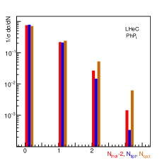
Figure 5: Normalized differential cross sections, with cuts $C_{0,\ldots,3}$, with respect to the number of light jets in hadronic top decay (red bars), in leptonic top decay (blue bars), and not associated with top decay (ocher bars).

In a top-pair production event in semileptonic channel for which (11) can be defined there must be at least two $b$ jets and at least two light ones. We then keep only the events satisfying the preselection cut

$$2\leq N_{b}~{},\qquad 2\leq N_{l}\leq 5~{}.$$ (12)

Here the requirement of at most five light jets is applied for computational simplicity since, out of the events with $N_{l}\geq 2$, approximately 98.5% have $N_{l}\leq 5$. Events fulfilling (12) can be reconstructed using (11).

We introduce a phase-space cut defining the photoproduction kinematic region,

$$C_{0}:\quad\left\{\begin{gathered}y(e^{-})\in PhP_{k},\quad k=I,II,III,\\ Q^{2}<3\,\mathrm{GeV}^{2},\;0<\xi<0.98,\\ \Delta R(j,j)>0.4,\end{gathered}\right.$$ (13)

where $e^{-}$ refers to the scattered electron, and the first line refers to the appropriate photoproduction region (10). In (13), $Q^{2}=-q_{\gamma}^{2}$ refers to the quasireal photon’s squared virtuality, and $\xi=q_{\gamma}^{0}/E_{e\mathrm{beam}}$ to the photon’s fraction of the electron-beam energy in the lab frame. We assume that the scattered electron must have an energy of at least 1.2 GeV to be detected at the very forward detector, which leads to the upper cut in $\xi$ in (13). The distributions of the scattered-electron lab-frame rapidity, $y(e^{-})$, and the photon energy fraction $\xi$ and $Q^{2}$ are shown in figure 4 in the three photoproduction regions (10) at the LHeC energy. $\Delta R(j,j)$ in (13) refers to the distance between any pair of jets, $\Delta R=\sqrt{(\Delta\eta)^{2}+(\Delta\varphi)^{2}}$.

	LHeC			FCC-he
	$PhP_{I}$	$PhP_{II}$	$PhP_{III}$	$PhP_{I}$	$PhP_{II}$	$PhP_{III}$
$p^{\perp}_{j\,\textrm{min}}$ [GeV]	10	15	20	15	20	25
$y_{b,\mathrm{min}}$	-0.5	-0.5	-0.5	-0.5	-0.5	-0.5
$y_{b,\mathrm{max}}$	3.0	3.0	3.0	3.0	2.7	2.7
$p^{\perp}_{b,\mathrm{min}}$ [GeV]	30	35	45	35	40	50
$p^{\perp}_{b,\mathrm{max}}$ [GeV]	$\infty$	$\infty$	$\infty$	$\infty$	200	200

Table 2: Parameters involved in the cuts $C_{0}$,…,$C_{4}$, equations (13),…,(17).

We identify the charged lepton $\ell$ from top decay with the leading-$p_{T}$ lepton. Both the LHeC and FCC-he detectors have a rapidity acceptance $|y|<4$ for muons. We use a cut for the charged lepton that essentially reflects that acceptance window,

$$C_{1}:\quad-2.8<y(\ell)<4,\quad|\vec{p}^{\perp}(\ell)|>5.0\,\mathrm{GeV},\quad|\vec{p}^{\perp}_{\mathrm{miss}}|>5.0\,\mathrm{GeV}.$$ (14)

We set a rapidity cut on all light jets that roughly follows the upper limit of the rapidity acceptance range for both the LHeC ($y<4.9$) and FCC-he ($y<5.2$) tracking systems. We identify the two leading $p_{T}$ light jets as originating from top decay, and we require them to satisfy a minimum $p_{T}$ cut.

$$C_{2}:\quad-2.0<y(j)<5.0,\quad|\vec{p}^{\perp}(J_{\mathrm{hdr}\,0})|,|\vec{p}^{\perp}(J_{\mathrm{hdr}\,1})|>p^{\perp}_{j\,\textrm{min}}.$$ (15)

Here $j$ refers to all jets except the two $b$-tagged ones with the highest transverse momenta. $J_{t_{\mathrm{hdr}}k}$ refers to the $p_{T}$-ordered collection of jets involved in the hadronic top decay ($k=0$, 1,…), as defined above. Eq. (15) requires the two hardest such ones to have $p_{T}>p^{\perp}_{j\,\mathrm{min}}$ as given in table 2. The remaining light jets $J_{\mathrm{hdr}\,k}$ with $k>1$, as well as the light jets $J_{\mathrm{lpt}\,k}$ arising from the leptonic decay and those not originating from a top decay, are required to satisfy $|\vec{p}^{\perp}|>10$ GeV. The differential cross sections with respect to light jet lab-frame rapidity and transverse momentum is shown in figure 6. The center-column panels in that figure refer to the two leading-$p_{T}$ jets originating in hadronic top decay. The right-column panels show the distributions for the leading supernumerary jets, $J_{\mathrm{hdr}\,2}$, $J_{\mathrm{lpt}\,0}$, $J_{\mathrm{spct}\,0}$. Notice that in this last case the distributions have a normalization deficit, since not all events contain supernumerary jets.

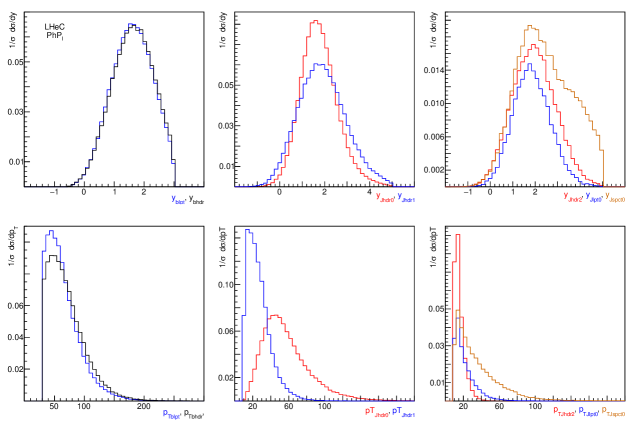
Figure 6: Normalized differential cross sections, with cuts $C_{0,\ldots,3}$, with respect to lab-frame rapidity (upper row) and transverse momentum (lower row). Left column: $b$ jet from leptonic, $J_{b0}$, and hadronic, $J_{b1}$, top decay. Central column: two leading-$p_{T}$ light jets from hadronic top decay. Right column: third leading-$p_{T}$ light jet from hadronic, and leading $p_{T}$ jet from leptonic top decay, and leading jet not originating in top decay.

As discussed in connection with the reconstruction of the top quarks, we identify the $b$ jets produced directly in the top decays with the two leading-$p_{T}$ $b$-tagged jets. The cuts in these jets’ kinematic variables are crucial to suppress the $tbW$ irreducible background. We adopt the following cuts,

$$C_{3}:\quad\left\{\begin{gathered}y_{b,\mathrm{min}}<y(J_{bk})<y_{b,\mathrm{max}}\\ p^{\perp}_{b,\mathrm{min}}<|\vec{p}^{\perp}(J_{bk})|<p^{\perp}_{b,\mathrm{max}}\end{gathered}\right.,\quad k=0,1,$$ (16)

where the relevant parameters are given in table 2. The parameter ranges in (16) are chosen so as to suppress the $tbW$ background as much as possible, but wide enough for the cuts to remain generic.

We introduce also a cut on the top masses,

$$C_{4}:\quad\left|m_{t\,\mathrm{hdr}}-m_{t}\right|^{2}+\left|m_{t\,\mathrm{lpt}}-m_{t}\right|^{2}<(\Delta m_{t})^{2},$$ (17)

where $m_{t\,\mathrm{hdr}}$, $m_{t\,\mathrm{lpt}}$ refer to the reconstructed masses of the hadronically and leptonically decaying top quarks, and where we take $m_{t}=172.5$ GeV, as already mentioned, and $\Delta m_{t}=30$ GeV. The mass distributions for the hadronically and leptonically decaying top quarks are shown in figure 7 (see the left panel). Also shown in the figure are the lab-frame rapidity and transverse momentum distributions for the hadronic and leptonic top quarks.

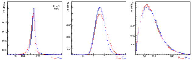
Figure 7: Normalized differential cross sections, with cuts $C_{0,\ldots,3}$, with respect to hadronically and leptonically decaying top quark mass (left panel), lab-frame rapidity (center panel) and transverse momentum (right panel).

Once the cuts $C_{0\text{--}4}$ have been applied, the cross sections for the $t\overline{t}$ photoproduction signal process (7), figure 1, and the $tbW$ irreducible background (8), figure 2, are found to be as follows,

$$\begin{array}[]{c|ccc|ccc|}&\lx@intercol\hfil\text{LHeC}\hfil\lx@intercol\vrule\lx@intercol&\lx@intercol\hfil\text{FCC-he}\hfil\lx@intercol\vrule\lx@intercol\\ {[}\text{fb}]&PhP_{I}&PhP_{II}&PhP_{III}&PhP_{I}&PhP_{II}&PhP_{III}\\ \hline\cr t\overline{t}&0.40&0.73&1.32&4.28&6.19&10.51\\ tbW&0.041&0.083&0.16&0.44&0.71&1.42\end{array}~{},$$ (18)

expressed in femtobarns. We notice here that the $tbW$ background has cross section at the parton level that is roughly 20% of the signal cross section at the LHeC, and roughly 35% at the FCC-he, the precise number depending on the photoproduction region. We designed the cuts $C_{0,\ldots,4}$ to reduce this background to levels below 15%. As seen in (18), the $tbW$ background is 10% of the signal in region $PhP_{I}$ and 11.3% in $PhP_{II}$ at both the LHeC and FCC-he. In region $PhP_{III}$ we have 12.2% at the LHeC and 13.5% at the FCC-he. The $tbW$ background proves to be the most difficult one to control. The irreducible background $tbqq$ (9), figure 3, leads to cross sections at the parton level that are at most 0.5% of those of the signal process $t\overline{t}$. At the detector level, when the cuts $C_{0,\ldots,4}$ are applied, these cross sections fall below the 0.1% level. We therefore neglect this background in what follows.

5 Further SM backgrounds

In the previous section the signal process (7) and two of its irreducible backgrounds, (8) and (9), both involving resonant top production, were discussed in detail. In this section we discuss several additional irreducible and reducible SM backgrounds. The $tbW$ production process (8) turns out to be the most important background, followed by single-top $tbq$ production (section 5.1), $Whq$ production (section 5.3), and $tbW$ again, in its reducible version (5.4). A summary of their cross sections relative to the signal process is given below in table 3.

5.1 Single-top photoproduction ($tbq$)

The single-top, or $tbq$, photoproduction irreducible background is of the form,

$$qe^{-}\rightarrow e^{-}t\overline{b}q^{\prime}+e^{-}\overline{t}bq^{\prime}\rightarrow e^{-}\,b\ell^{+}\nu_{\ell}\,\overline{b}q^{\prime}+e^{-}\,\overline{b}\ell^{-}\overline{\nu}_{\ell}\,bq^{\prime}~{}.$$ (19)

With all possible lepton- and quark- flavor combinations taken into account, this process is given by 320 Feynman diagrams. For this process to pass the preselection cut (12), an additional parton must be radiated. We may obtain that additional jet in the final state by QCD showering, or by considering the photoproduction of the final states (19) with an additional gluon. For the purpose of obtaining the cross section, either process, or an appropriately matched combination of the two, leads to the same result.

The process of $tbqg$ photoproduction is determined by 1800 Feynman diagrams distributed among 32 flavor channels. The cross section for (19), however, is dominated by subprocesses with an initial valence quark undergoing a Cabibbo-allowed transition. In particular, the cross section for final states with an antilepton $\ell^{+}$ is twice as large as that for final states with $\ell^{-}$, since the former involve $u\rightarrow d$, while the latter involve $d\rightarrow u$. Judicious choice of the 10 flavor channels with the largest cross sections leads to a reduction of the number of diagrams to 585 without loss of numerical precision. From the diagrams for $tbqq$ photoproduction in figure 3 we can obtain diagrams for $tbqg$ by crossing the initial gluon to the final state, and one final-state light quark to the initial state. Further diagrams can be obtained from those by reattaching the final gluon to other colored lines in the diagram.

Full simulation, including the cuts $C_{0\text{--}4}$, leads to the cross sections for this process,

$$\begin{array}[]{c|ccc|ccc|}&\lx@intercol\hfil\text{LHeC}\hfil\lx@intercol\vrule\lx@intercol&\lx@intercol\hfil\text{FCC-he}\hfil\lx@intercol\vrule\lx@intercol\\ {[}\text{fb}]&PhP_{I}&PhP_{II}&PhP_{III}&PhP_{I}&PhP_{II}&PhP_{III}\\ \hline\cr tbq&0.014&0.032&0.061&0.039&0.072&0.13\\ tbqg&0.017&0.029&0.046&0.041&0.060&0.091\end{array}~{},$$ (20)

expressed in femtobarns. We see that this background constitutes 4% of the signal cross section at the LHeC, and 1% at the FCC-he.

5.2 No-top irreducible background: gluon-initiated processes

In this section we consider irreducible backgrounds to the signal process (7), described by Feynman diagrams not containing top lines. We begin by discussing the processes with $ge^{-}$ initial states; the ones with initial $qe^{-}$, with $q$ a light quark, are the topic of the next subsection.

We consider processes with the same initial and final state as the signal one (7),

$$ge^{-}\rightarrow e^{-}\,b\ell^{+}\nu_{\ell}\,\overline{b}\overline{q}_{u}q_{d}+e^{-}\,bq_{u}\overline{q}_{d}\,\overline{b}\ell^{-}\overline{\nu}_{\ell}~{},$$ (21)

but described by Feynman diagrams without internal top lines. Taking into account the four quark-flavor channels and the duplication of the number of diagrams in the $e^{-}$ lepton channel, there are 7920 diagrams for the process (21), without $t$ lines and with one QCD vertex, in the photoproduction regime. We denote that set of diagrams QCD¹. There is also a set of 1880 diagrams without $t$ lines and with three QCD vertices, which we denote QCD³. Some diagrams for the process (21) are illustrated in figure 8.

Figure 8: Representative unitary-gauge Feynman diagrams for the photoproduction of (a) $WWb\overline{b}$ in semileptonic mode, (b) $Wg^{*}qq$, (c) $Whqq$, $WZqq$, $W\gamma^{*}qq$. These diagrams belong to the set QCD${}^{1}_{bbg}$, QCD³, QCD${}^{1}_{qqg}$ respectively, see text.

We consider first the diagrams with only one QCD vertex, set QCD¹. We divide that set into two subsets, $\mathrm{QCD}^{1}=\mathrm{QCD}^{1}_{bbg}\cup\mathrm{QCD}^{1}_{qqg}$, with QCD${}^{1}_{bbg}$ the set of diagrams in which the QCD vertex is $bbg$, and QCD${}^{1}_{qqg}$ that of diagrams with a $qqg$ vertex, with $q$ any light quark. The set QCD${}^{1}_{bbg}$ contains 3240 diagrams, and QCD${}^{1}_{qqg}$ contains 4680 diagrams. The set QCD${}^{1}_{bbg}$ has a cross section that is between 70% and 90% of the cross section for the entire set QCD¹, depending on the energy and photoproduction region, with the set QCD${}^{1}_{qqg}$ providing the rest of the cross section.

The cross section obtained from the set QCD${}^{1}_{bbg}$ is dominated by the contribution from the diagrams for the process (21) with $WWbb$ intermediate state, $ge^{-}\rightarrow e^{-}b\overline{b}\,W^{+}W^{-}$, as illustrated in figure 8 (a). The photoproduction of $WWbb$ is given by 720 diagrams and yields more than 90% of the QCD${}^{1}_{bbg}$ cross section. The cross sections for QCD${}^{1}_{bbg}$ are small relative to the signal process already at the parton level, with the largest percentage fraction obtained at the FCC-he energy and in the $PhP_{III}$ region, and found to be 3%. Even in that case however, at the detector-simulation level and with the cuts from section 4, the cross section for QCD${}^{1}_{bbg}$ is found to amount to 0.08% of the signal process, so we consider it negligible.

The set of diagrams QCD${}^{1}_{qqg}$ gives a smaller fraction of the cross section for the entire set QCD¹, representing from 20% in the region $PhP_{I}$ to 30% in $PhP_{III}$ at the LHeC energy, and about 12% at the FCC-he. The main contribution to the cross section from this set originates in the doubly resonant production of $hWqq$, followed by the leptonic decay of $W$ and $h\rightarrow b\overline{b}$. This process is given by 320 Feynman diagrams, with a representative example shown in figure 8 (c). A smaller contribution to the cross section originates in the photoproduction of $ZWqq$, also shown in the figure. This process is given by 1000 Feynman diagrams. Its cross section is at most one-third of that for $hWqq$ (in $PhP_{I}$ at the LHeC) to less than 1% of $hWqq$ at the FCC-he. There is a set of less resonant processes similar to $hWqq$, such as $h\ell\nu qq$ and $Z\ell\nu qq$ photoproduction, that yield much smaller cross sections. The remaining diagrams in the set QCD${}^{1}_{qqg}$ not considered so far involve the vertex $\gamma^{*}\rightarrow b\overline{b}$. These are 2040 diagrams that yield a cross section much smaller than $hWqq$ photoproduction, and can therefore be neglected. Just as with the processes described by QCD${}^{1}_{bbg}$, the contribution of QCD${}^{1}_{qqg}$ to the cross section is negligibly small compared to the signal cross section.

The set of diagrams QCD³, illustrated in figure 8 (b), is at most singly resonant and leads to small corrections to the cross sections obtained from the set QCD¹, so we will not consider it further here. We mention, however, that this set of diagrams is closely related to the reducible background discussed below in section 5.6. As an illustration of this fact we notice that diagram 8 (b) is the same as 11 (b) with $q=b$. Thus, the cross section for the QCD³ processes is actually taken into account when showering the backgrounds in section 5.6.

5.3 No-top irreducible background: quark-initiated processes

In this section we turn our attention to processes with one less light parton in the final state as the signal one (7),

$$qe^{-}\rightarrow e^{-}qb\overline{b}\ell\nu_{\ell},$$ (22)

and described by Feynman diagrams without internal top lines. Taking into account the four quark-flavor channels and the duplication of the number of diagrams in the $e^{-}$ lepton channel, there are 3320 diagrams for process (22), without $t$ lines, at lowest QCD order and in the photoproduction regime. A few of those diagrams are illustrated in figure 9.

Figure 9: Sample unitary-gauge Feynman diagrams for the photoproduction of $Whq$, $WZq$ in semileptonic mode.

The cross section for the processes (22) is strongly dominated by $Whq$, and to a lesser extent $WZq$, associated photoproduction as illustrated in the figure. In fact, these doubly resonant processes account for about 97% of the cross section for (22), with $Whq$ alone yielding 90% of the total.

If we restrict ourselves to those doubly resonant processes, the number of diagrams is reduced to 36 per flavor channel. However, in order to compute the cross section, it is enough to consider processes with a valence quark in the initial state and a Cabibbo-allowed flavor transition, and only one lepton flavor,

$$ue^{-}\rightarrow e^{-}db\overline{b}\overline{\mu}\nu_{\mu},\quad de^{-}\rightarrow e^{-}ub\overline{b}\mu\overline{\nu}_{\mu},$$ (23)

and multiply the cross section $\times 2.11$ at the LHeC and $\times 2.28$ at the FCC-he.

The numerical results for the cross section for this irreducible background are as follows,

$$\begin{array}[]{c|ccc|ccc|}&\lx@intercol\hfil\text{LHeC}\hfil\lx@intercol\vrule\lx@intercol&\lx@intercol\hfil\text{FCC-he}\hfil\lx@intercol\vrule\lx@intercol\\ {[}\text{fb}]&PhP_{I}&PhP_{II}&PhP_{III}&PhP_{I}&PhP_{II}&PhP_{III}\\ \hline\cr Whq+WZq&0.007&0.014&0.018&0.011&0.016&0.013\end{array}~{}.$$ (24)

These cross sections are rather small, though not negligible, at the LHeC, where they constitute 1.8% of the signal cross section after cuts, but much less significant at the FCC-he where they are 0.2% of the signal.

5.4 Photoproduction of $tbW$ as reducible background

In the LHeC simulation in Delphes 3.4.2 with default parameters, the $b$-tagging algorithm only operates on jets with lab.-frame absolute rapidity $|y(j)|<3$, and $p_{T}>0.5$ GeV. In the case of the FCC-he detector simulation, $b$ tagging is restricted to $|y(j)|<4$, and $p_{T}>4.0$ GeV. It is then possible to have $tbW$ events in which one $b$-jet with $|y(j_{b})|<y_{\mathrm{max}}=3$, 4 is tagged and passes the cuts (16), whereas the other $b$-jet has $y(j_{b})>3$ and is therefore not tagged, but passes the cuts (15) for light jets. Under those conditions, if a light jet is mistagged and satisfies the conditions (16), the event could pass the cuts. We conclude, then, that the process $tbW$ has a reducible component that we must consider. We estimate the cross section for this process by requiring at the parton level that one $b$ quark be inside the flavor-tagging region and the other one outside. The cross sections we obtain are

$$\begin{array}[]{c|ccc|ccc|}&\lx@intercol\hfil\text{LHeC}\hfil\lx@intercol\vrule\lx@intercol&\lx@intercol\hfil\text{FCC-he}\hfil\lx@intercol\vrule\lx@intercol\\ {[}\text{fb}]&PhP_{I}&PhP_{II}&PhP_{III}&PhP_{I}&PhP_{II}&PhP_{III}\\ \hline\cr tbW_{\mathrm{red}}&0.004&0.006&0.013&0.008&0.007&0.005\end{array}~{}.$$ (25)

We conclude that this reducible component of the $tbW$ background constitutes about 1% of the signal cross section at the LHeC in all three photoproduction regions, and not more than 0.2% at the FCC-he.

5.5 Reducible backgrounds: quark-initiated processes

Figure 10: Sample unitary-gauge Feynman diagrams for quark-initiated reducible background processes including photoproduction of (a) $Wq$, (b) $Wqqq$, (c) $WWq$, (d) $WZq$/$W\gamma^{*}q$.

The quark-initiated photoproduction processes with one charged lepton, missing transverse energy and jets in the final state are described by Feynman diagrams with $N_{p}=N_{g}+N_{q}$ partons in the final state, where $N_{g}\geq 0$ is the number of gluons and $N_{q}\geq 1$ odd is the number of quarks, and exactly $N_{QCD}$ strong and ($N_{p}+3-N_{QCD}$) electroweak vertices. We will restrict ourselves to $N_{q}=1,$ 3, since larger values lead to processes with very small cross sections.

For $N_{q}=1$ we obtain leptonic single-$W$ production associated with at least one jet, as illustrated by the Feynman diagram in figures 10 (a), (b). For the purpose of estimating the cross section we take into account at the parton level only diagrams with $N_{QCD}=0$, such as 10 (a), and deal with QCD radiation only through Pythia showering. Thus, when all possible lepton- and quark- flavor combinations are allowed for, we have 160 diagrams analogous to that of figure 10 (a) with exactly one final-state quark and four electroweak vertices. The cross sections are quite small, as this background represents 0.2% of the signal process at the LHeC, region $PhP_{I}$, and less than 0.1% in the other regions. At the FCC-he this background essentially vanishes, due to the higher purity of the $b$-tagging algorithm.

For $N_{q}=3$, at lowest order in QCD, we have diagrams with three final-state quarks and six electroweak vertices as shown in figures 10 (c) and (d). There are 40500 such Feynman diagrams when all 320 possible quark- and lepton- flavor combinations are taken into account. Out of the many physical processes contributing to the cross section for this background, the dominant ones are the doubly resonant $WW$ production, illustrated in figure 10 (c), and $WZ$ production, shown in 10 (d) together with the singly resonant production of $W\gamma^{*}$. Numerically, the cross sections for these processes are typically a few percent of those for the $N_{q}=1$ processes, therefore negligibly small. These results also strongly suggest that we do not need to consider reducible backgrounds with $N_{q}\geq 5$.

5.6 Reducible backgrounds: gluon-initiated processes

The gluon-initiated photoproduction processes with one charged lepton, missing transverse energy and jets in the final state are described by Feynman diagrams with $N_{p}=N_{g}+N_{q}$ partons in the final state, where $N_{g}\geq 0$ is the number of gluons and $N_{q}\geq 2$ even is the number of quarks, and exactly $N_{QCD}$ strong and ($N_{p}+3-N_{QCD}$) electroweak vertices. We will restrict ourselves to $N_{q}=2,$ 4, since larger values lead to processes with very small cross sections.

For $N_{q}=2$ we obtain leptonic single-$W$ production associated with at least two jets, as illustrated by the Feynman diagram in figure 11 (a), (b). As in the case of quark-initiated processes, we allow for further QCD radiation only through Pythia showering. Thus, when all possible lepton- and quark- flavor combinations are considered, we have 200 diagrams analogous to that of figure 11 (a) with exactly two final-state quarks, one strong and four electroweak vertices.

Figure 11: Sample unitary-gauge Feynman diagrams for gluon-initiated reducible background processes including photoproduction of (a) $Wqq$, (b) Wqqqq, (c) $WWqq$, (d) $WZqq$/$W\gamma^{*}qq$.

The cross sections obtained for these processes with the cuts described in section 4 are negligibly small. This background represents less than 0.1% of the signal process at the LHeC, region $PhP_{I}$, and much less than that in the other regions. At the FCC-he this background essentially vanishes, due to the higher purity of the $b$-tagging algorithm.

For $N_{q}=4$, at lowest order in QCD, we have diagrams with four final-state quarks, one strong and six electroweak vertices as shown in figures 11 (c) and (d). There are 64800 such Feynman diagrams when all 96 possible quark- and lepton- flavor combinations are taken into account. Out of the many physical processes contributing to the cross section for this background, the dominant ones are the doubly resonant $WW$ production, illustrated in figure 11 (c), and $WZ$ production, shown in 11 (d) together with the singly resonant production of $W\gamma^{*}$. Numerically, the parton-level cross sections for these processes are typically less than 1% of those for the $N_{q}=2$ processes. Thus, the contributions of these processes to the background cross section are negligibly small. These results also strongly suggest that we do not need to consider reducible backgrounds with $N_{q}\geq 6$.

6 Results for effective couplings

For the computation of the cross section as a function of the effective couplings $\widetilde{C}_{uB}^{33}\rule{0.0pt}{12.0pt}$, $\widetilde{C}_{\varphi q}^{(-)33}\rule{0.0pt}{12.0pt}$, we simulated the top-pair photoproduction process in $pe^{-}$ collisions with MG5, Pythia 6, and Delphes 3 as described in section 4. The effective operators (3) were implemented in MagGraph 5 by means of the program FeynRules version 2.0.33 [52].

As discussed above in section 3, there are 180 diagrams for semileptonic top-pair photoproduction and decay in the SM with Cabibbo mixing, allowing for all possible quark- and (light) lepton- flavor combinations. When the effective operators are included, additional diagrams enter the computation. If we include only the operator $Q_{uB}^{33}$, there are 40 additional diagrams with one effective vertex, for a total of 220 diagrams. If we include only the operator $Q_{\varphi Q}^{(-)33}$, there are 360 additional diagrams with one effective vertex and 180 with two such vertices, for a total of 720 diagrams. Finally, if we take into account both operators, then there are 400 diagrams with one effective vertex, 260 with two and 40 with three effective vertices, for a total of 880 diagrams. Representative diagrams with one, two and three effective vertices are shown in figure 12.

Figure 12: Representative unitary-gauge Feynman diagrams with one, two and three anomalous effective vertices.

Diagrams with one, two and three effective vertices entering the amplitude for (7), contribute to it at $\mathcal{O}(\Lambda^{-n})$ with $n=2,$ 4 and 6, respectively. In fact, once the top propagator dependence on effective couplings through the top decay width is taken into account, the scattering amplitude is given as a power series of $\Lambda^{-2}$. We remark that diagrams with two effective vertices must be kept in the amplitude since, through their interference with SM diagrams, they make contributions to the cross section of the same order, $\mathcal{O}(\Lambda^{-4})$, as the square of diagrams with only one effective vertex. We have actually taken into account the contributions from diagrams with three effective vertices in our calculation as well as the dependence of the top decay width on the effective couplings, but we have explicitly verified in all cases that the contribution to the cross section from terms of order higher than $\mathcal{O}(\Lambda^{-4})$ is actually negligible for values of the effective couplings within the bounds given below. (We remark here, parenthetically, that the contributions to the cross section at order $1/\Lambda^{4}$ from dimension-eight operators interfering with the SM are currently unknown and constitute an inherent uncertainty of the EFT analysis at dimension six.)

6.1 Methodology and assumptions

In order to obtain bounds on the effective couplings, we consider the ratio of the cross section $\sigma_{\mathrm{eff}}(\{\widetilde{C}_{\mathcal{O}}\})$ obtained from the Lagrangian (1) at tree level to the SM cross section $\sigma_{\mathrm{SM}}=\sigma_{\mathrm{eff}}(\{0\})$

$$R=\frac{\sigma_{\mathrm{eff}}(\{\widetilde{C}_{\mathcal{O}}\})}{\sigma_{\mathrm{SM}}},$$ (26)

where $\{\widetilde{C}_{\mathcal{O}}\}$ is the set of anomalous coupling constants. For a given relative experimental uncertainty $\varepsilon_{\mathrm{exp}}$, the region of allowed values for the effective couplings $\{\widetilde{C}_{\mathcal{O}}\}$ is determined at the $n_{\sigma}\;\sigma$ ($n_{\sigma}=1,$ 2,…) level by the inequalities

$$R\lessgtr 1\pm n_{\sigma}\varepsilon_{\mathrm{exp}}.$$ (27)

Since only three real effective couplings enter the Lagrangian for the processes considered here, we can parametrize the ratio (26) as

$$R=1+a_{1}\,\widetilde{C}_{uB\,r}^{33}\rule{0.0pt}{12.0pt}+a_{2}\left(\widetilde{C}_{uB\,r}^{33}\rule{0.0pt}{12.0pt}\right)^{2}+a^{\prime}_{2}\left(\widetilde{C}_{uB\,i}^{33}\rule{0.0pt}{12.0pt}\right)^{2}+b_{1}\,\widetilde{C}_{\varphi q}^{(-)33}\rule{0.0pt}{12.0pt}+b_{2}\left(\widetilde{C}_{\varphi q}^{(-)33}\rule{0.0pt}{12.0pt}\right)^{2}+c\,\widetilde{C}_{uB\,r}^{33}\rule{0.0pt}{12.0pt}\widetilde{C}_{\varphi q}^{(-)33}\rule{0.0pt}{12.0pt}+\cdots$$ (28)

We obtain allowed intervals on the effective couplings by substituting (28) in (27) with only one of the couplings in (28) taken to be nonzero. Similarly, we consider also allowed two-coupling regions for pairs of effective couplings by setting the remaining one to zero in (28). The parameters in (28) are determined from an extensive set of Monte Carlo simulations at the detector level, for each energy and photoproduction region, to which (28) is fitted. Once those parameters are known, (27) yields the desired one- or two-dimensional limits on the effective couplings being considered. The consistency condition that the contribution to the cross section from terms of $O\left(\Lambda^{-6}\right)$ and higher in (1) be negligibly small entails on the parametrizations (28) the requirement that the terms of $O(\widetilde{C}^{3})$ and higher must be correspondingly negligible within the allowed region determined by (27). We check this consistency condition in all cases considered below.

The cross-section ratio (26) depends on the renormalization and factorization scales, for moderate values of the effective couplings, much more weakly than the cross sections themselves. This was previously noticed, in a rather different context, in [14] (see section IV C of that reference). Thus, the bounds on the effective couplings obtained from (27) are therefore largely independent of those scales.

	LHeC			FCC-he
(%)	$PhP_{I}$	$PhP_{II}$	$PhP_{III}$	$PhP_{I}$	$PhP_{II}$	$PhP_{III}$	section
$tbW$	10.3	11.3	12.2	10.3	11.4	13.5	4
$tbq$	3.6	4.4	4.6	0.9	1.2	1.3	5.1
$Whq+WZq$	1.8	1.8	1.4	0.2	0.2	0.2	5.3
$tbW$(red.)	1.0	0.8	1.0	0.2	0.1	0.05	5.4
statistical	5.0	3.7	2.8	1.5	1.3	1.0	4
RMS	12.2	12.8	13.4	10.5	11.5	13.6

Table 3: Background-to-signal ratios expressed as percentages of the signal cross section, for the four main background processes and statistical uncertainty. “RMS” refers to the sum in quadrature of the previous lines.

In order to obtain bounds on the effective couplings through (27), below we assume $\varepsilon_{\mathrm{exp}}$ to take values within a certain interval, which is motivated by estimating the uncertainties in the signal cross section in our Monte Carlo simulations through the addition in quadrature of the statistical uncertainty and the backgrounds cross sections, as summarized in table 3. In view of those results, we will assume total measurement uncertainties of $\varepsilon_{\mathrm{exp}}=$12%, 15%, 18%. The first value would be applicable to photoproduction region $PhP_{I}$, especially at the FCC-he, the second and third value could be applicable in the other photoproduction regions. The largest value of 18% is the one used in [16]. More importantly, once bounds on the anomalous couplings have been established for these three uncertainty values, results for other $\varepsilon_{\mathrm{exp}}$ can be obtained by interpolation.

6.2 Bounds on $\boldsymbol{\widetilde{C}_{\varphi q}^{(-)33}\rule{0.0pt}{12.0pt}}$

We obtain bounds on the left-handed vector $tbW$ coupling from Monte Carlo simulations as described previously in this section. In table 4 we report the single-coupling bounds for $\widetilde{C}_{\varphi q}^{(-)33}\rule{0.0pt}{12.0pt}$ obtained from (27) at the LHeC and FCC-he energies, at the three photoproduction regions, at the $1\sigma$ level, for three values of the assumed experimental uncertainty.

$\widetilde{C}_{\varphi q}^{(-)33}\rule{0.0pt}{12.0pt}$, 68% C.L.
	LHeC			FCC-he
$\varepsilon_{\mathrm{exp}}$	$PhP_{I}$	$PhP_{II}$	$PhP_{III}$	$PhP_{I}$	$PhP_{II}$	$PhP_{III}$
12%	-0.11,0.080	-0.056,0.049	-0.039,0.035	-0.11,0.081	-0.061,0.051	-0.039,0.035
15%	-0.14,0.098	-0.072,0.060	-0.049,0.043	-0.14,0.099	-0.078,0.063	-0.049,0.043
18%	-0.18,0.11	-0.089,0.071	-0.060,0.052	-0.18,0.12	-0.097,0.074	-0.060,0.051

Table 4: Single-coupling limits on the charged-current effective coupling $\widetilde{C}_{\varphi q}^{(-)33}\rule{0.0pt}{12.0pt}$, at 68% C.L., at the LHeC and FCC-he energies, in three photoproduction phase-space regions and for three assumed experimental uncertainties.

Clearly, the largest sensitivity is obtained in region $PhP_{III}$. Indeed, the anomalous coupling $\widetilde{C}_{\varphi q}^{(-)33}\rule{0.0pt}{12.0pt}$ constitutes a perturbation $\delta f_{V}^{L}$ to the SM CC coupling $f_{V}^{L}=1+\delta f_{V}^{L}$ and, therefore, it also perturbs the gauge cancellation discussed above under eq. (7). Thus, the sensitivity is largest in region $PhP_{III}$ where the cancellation is strongest. For that region we report 95% C.L. results both for the LHeC and the FCC-he in table 5.

	$\widetilde{C}_{\varphi q}^{(-)33}\rule{0.0pt}{12.0pt}$, $PhP_{III}$, 95% C.L.
$\varepsilon_{\mathrm{exp}}$	LHeC	FCC-he
12%	-0.083,0.067	-0.083,0.067
15%	-0.11,0.083	-0.11,0.082
18%	-0.14,0.098	-0.14,0.097

Table 5: Single-coupling limits on the charged-current effective coupling $\widetilde{C}_{\varphi q}^{(-)33}\rule{0.0pt}{12.0pt}$, at 95% C.L., at the LHeC and FCC-he energies, in photoproduction region $PhP_{III}$ and for three assumed experimental uncertainties.

We see from tables 4, 5 that the sensitivities obtained at the LHeC and at the FCC-he are essentially the same. (In appendix C we give the bounds for LHeC, $PhP_{III}$, in terms of $C_{\varphi q}^{(-)33}\rule{0.0pt}{12.0pt}$ for the purpose of comparison with other bounds in the literature.) Finally, the fit parameters from (28) are given by,

$$\begin{array}[]{ccc}&b_{1}&b_{2}\\ \mbox{LHeC:}&3.259&4.407\\ \mbox{FCC-he:}&2.263&4.552\end{array},$$ (29)

for the photoproduction region $PhP_{III}$.

A fit similar to (29) for the main background $tbW$ yields $b_{1}=2.221$, $b_{2}=1.650$ at the LHeC, and $b_{1}=2.275$, $b_{2}=1.663$ at the FCC-he. It should be taken into account that, due to the fact that the cross section for $tbW$ is suppressed by the cuts (13)–(17), these coefficients are subject to a larger numerical uncertainty than those for the signal in (29). Let us consider, for concreteness, the range of values for $\widetilde{C}_{\varphi q}^{(-)33}\rule{0.0pt}{12.0pt}$ in table 4 corresponding to a variation $\Delta\sigma_{t\overline{t}}/\sigma_{t\overline{t}}=12\%$ at the LHeC in region $PhP_{III}$. The parameters $b_{1,2}$ given above for $\sigma_{tbW}$ imply a corresponding variation $\Delta\sigma_{tbW}/\sigma_{tbW}=8\%$. Relative to the signal cross section, see (18), the variation is small $\Delta\sigma_{tbW}/\sigma_{t\overline{t}}=0.97\%$, for a total uncertainty of $\sqrt{0.12^{2}+0.0097^{2}}=12.04\%$. Similarly small results are found in the other regions, and at the FCC-he energy.

It is of interest to compare our results for $\widetilde{C}_{\varphi q}^{(-)33}\rule{0.0pt}{12.0pt}$ with those reported by CMS. A recent measurement of the single-top production cross section used to set bounds on $\delta f_{V}^{L}$ is given in [32]. From figure 6 of [32] we obtain the following limits at 1- and 2-$\sigma$ significance:

$$\begin{array}[]{lcc}&\mbox{68\% C.L.}&\mbox{95\% C.L.}\\ \mbox{CMS:}&-0.024<\delta f_{V}^{L}<0.094&-0.062<\delta f_{V}^{L}<0.132~{},\end{array}$$ (30)

with $f_{V}^{L}=1+\delta f_{V}^{L}$ and, as shown above, $\delta f_{V}^{L}=\widetilde{C}_{\varphi q}^{(-)33}\rule{0.0pt}{12.0pt}$. We compare the limits we obtain in region $PhP_{III}$ in tables 4 and 5 to the CMS result (30) by comparing the interval lengths. We see that at 68% C.L. our limits are more restrictive than those from (30) for all three values of $\varepsilon_{\mathrm{exp}}$ considered in the table. At $\varepsilon_{\mathrm{exp}}=12\%$, in particular, the interval length in table 4 is smaller than that in (30) by roughly one-third. At 95% C.L. our results give a tighter bound for $\varepsilon_{\mathrm{exp}}=12\%$, an equally tight bound at $\varepsilon_{\mathrm{exp}}=15\%$ and somewhat looser bounds at $\varepsilon_{\mathrm{exp}}=18\%$.

6.3 Bounds on $\boldsymbol{\widetilde{C}_{uB}^{33}\rule{0.0pt}{12.0pt}}$: single-coupling bounds

We obtain bounds on the dipole $tt\gamma$ couplings from Monte Carlo simulations as previously described in this section. In table 6 we report the single-coupling bounds for $\widetilde{C}_{uB\,r}^{33}\rule{0.0pt}{12.0pt}$ obtained from (27) at the LHeC and FCC-he energies, in the three photoproduction regions, at the $1\sigma$ level, for three values of the assumed experimental uncertainty.

$\widetilde{C}_{uB\,r}^{33}\rule{0.0pt}{12.0pt}$, 68%C.L.
	LHeC			FCC-he
$\varepsilon_{\mathrm{exp}}$	$PhP_{I}$	$PhP_{II}$	$PhP_{III}$	$PhP_{I}$	$PhP_{II}$	$PhP_{III}$
12%	-0.041,0.049	-0.063,0.084	-0.13,0.58	-0.040,0.049	-0.061,0.090	-0.13,0.52
15%	-0.050,0.063	-0.077,0.120	-0.16,0.61	-0.048,0.063	-0.075,0.130	-0.15,0.54
18%	-0.059,0.078	-0.090,0.150	-0.18,0.64	-0.057,0.080	-0.088,0.510	-0.17,0.57

Table 6: Single-coupling limits on the effective coupling $\widetilde{C}_{uB\,r}^{33}\rule{0.0pt}{12.0pt}$, at 68% C.L., at the LHeC and FCC-he energies, in three photoproduction phase-space regions and for three assumed experimental uncertainties.

Similarly, in table 7 we show the bounds for the coupling $\widetilde{C}_{uB\,i}^{33}$.

$\widetilde{C}_{uB\,i}^{33}\rule{0.0pt}{12.0pt}$, 68%C.L.
	LHeC			FCC-he
$\varepsilon_{\mathrm{exp}}$	$PhP_{I}$	$PhP_{II}$	$PhP_{III}$	$PhP_{I}$	$PhP_{II}$	$PhP_{III}$
12%	$\pm$0.15	$\pm$0.18	$\pm$0.28	$\pm$0.13	$\pm$0.18	$\pm$0.25
15%	$\pm$0.16	$\pm$0.21	$\pm$0.32	$\pm$0.15	$\pm$0.20	$\pm$0.28
18%	$\pm$0.18	$\pm$0.23	$\pm$0.35	$\pm$0.17	$\pm$0.22	$\pm$0.31

Table 7: Single-coupling limits on the effective coupling $\widetilde{C}_{uB\,i}^{33}\rule{0.0pt}{12.0pt}$, at 68% C.L., at the LHeC and FCC-he energies, in three photoproduction phase-space regions and for three assumed experimental uncertainties.

Clearly, the largest sensitivity to $\widetilde{C}_{uB}^{33}$ is obtained in region $PhP_{I}$. This is due to two different mechanisms. First, the fact that the SM is close to an infrared divergence at $Q^{2}=0$ and, therefore, as $Q^{2}$ decreases the SM cross section grows much faster than the dipolar cross section, which is infrared finite. This causes the sensitivity to both $\widetilde{C}_{uB\,r}^{33}\rule{0.0pt}{12.0pt}$, $\widetilde{C}_{uB\,i}^{33}\rule{0.0pt}{12.0pt}$ to decrease as we go from $PhP_{I}$ to $PhP_{III}$. Second, as seen in figure 4 (see left panel), the rapidity distribution of the scattered electron is more sharply peaked in $PhP_{III}$ than in $PhP_{I}$, thus leading to a smaller interference with the dipolar amplitude that leads to a flat distribution for $y(e^{-})$. This causes a reduction in the sensitivity to $\widetilde{C}_{uB\,r}^{33}\rule{0.0pt}{12.0pt}$ in $PhP_{III}$ as compared to $PhP_{I}$.

The results obtained in region $PhP_{I}$ are also given at the 2$\sigma$ level in table 8. (In appendix C we give the bounds for LHeC, $PhP_{I}$, in terms of $C_{uB\,r}^{33}\rule{0.0pt}{12.0pt}$ for the purpose of comparison with other bounds in the literature.)

	$PhP_{I}$,95%C.L.
	$\widetilde{C}_{uB\,r}^{33}\rule{0.0pt}{12.0pt}$		$\widetilde{C}_{uB\,i}^{33}\rule{0.0pt}{12.0pt}$
$\varepsilon_{\mathrm{exp}}$	LHeC	FCC-he	LHeC	FCC-he
12%	-0.076,0.11	-0.074,0.12	$\pm$0.21	$\pm$0.19
15%	-0.092,0.17	-0.088,0.21	$\pm$0.23	$\pm$0.21
18%	-0.110,0.60	-0.100,0.53	$\pm$0.25	$\pm$0.23

Table 8: Single-coupling limits on the effective couplings $\widetilde{C}_{uB\,r}^{33}\rule{0.0pt}{12.0pt}$, $\widetilde{C}_{uB\,i}^{33}\rule{0.0pt}{12.0pt}$, at 95% C.L., at the LHeC and FCC-he energies, in photoproduction region $PhP_{I}$ and for three assumed experimental uncertainties.

Finally, the fit parameters from (28) are given by,

$$\begin{array}[]{cccc}&a_{1}&a_{2}&a^{\prime}_{2}\\ \mbox{LHeC:}&-2.733&5.547&5.585\\ \mbox{FCC-he:}&-2.778&6.509&6.586\end{array},$$ (31)

for the photoproduction region $PhP_{I}$.

In photoproduction region $PhP_{I}$ the results analogous to (31) for the main background process $tbW$ are given by $a_{1}=-0.177$, $a_{2}=0.0599$, $a^{\prime}_{2}=0.198$ at the LHeC and $a_{1}=-0.135$, $a_{2}=0.271$, $a^{\prime}_{2}=0.364$ at the FCC-he. These numbers are subject to a larger numerical uncertainty than those for the signal in (31), because the cross section for $tbW$ is suppressed by the cuts (13)–(17). In this case, the range of values for $\widetilde{C}_{uB\,r}^{33}\rule{0.0pt}{12.0pt}$ in table 6 corresponding to a variation $\Delta\sigma_{t\overline{t}}/\sigma_{t\overline{t}}=12\%$ at the LHeC in region $PhP_{I}$, leads to $\Delta\sigma_{tbW}/\sigma_{tbW}=0.8\%$ which, relative to the signal cross section, corresponds to $\Delta\sigma_{tbW}/\sigma_{t\overline{t}}=0.08\%$. Similarly negligibly small results are found in the other regions, and at the FCC-he energy.

We mention that although not reported in detail here, we have carried out a complete parton-level analysis of the sensitivity to $\widetilde{C}_{uB\,r}^{33}\rule{0.0pt}{12.0pt}$, $\widetilde{C}_{uB\,i}^{33}\rule{0.0pt}{12.0pt}$ in all three photoproduction regions. In the case of region $PhP_{I}$, the limits obtained on those couplings are essentially the same as those obtained previously in [16] in the framework of the EPA. On the other hand, it is of interest to compare the bounds obtained here from parametric detector-level Monte Carlo simulations to those from the parton-level analysis of [16]. From table IX of [16], and using the relation (6) between $\kappa$, $\widetilde{\kappa}$ and $\widetilde{C}_{uB\,r}^{33}\rule{0.0pt}{12.0pt}$, $\widetilde{C}_{uB\,i}^{33}\rule{0.0pt}{12.0pt}$, we find that, assuming $\varepsilon_{\mathrm{exp}}=10$% experimental uncertainty and at 1$\sigma$ C.L., we have,

$$-0.022<\widetilde{C}_{uB\,r}^{33}<0.026,\quad|\widetilde{C}_{uB\,i}^{33}|<0.10.$$ (32)

From the same table in [16] we find the following bounds also at 1$\sigma$ and at $\varepsilon=18$% experimental uncertainty,

$$-0.039<\widetilde{C}_{uB\,r}^{33}<0.047,\quad|\widetilde{C}_{uB\,i}^{33}|<0.14.$$ (33)

These bounds are tighter than the comparable ones in tables 6, 7, as expected since the analysis in [16] is carried out at the parton level only. We notice, however, that the more complete analysis performed here yields 68% C.L. intervals for $\widetilde{C}_{uB\,r}^{33}$ that are slightly less than 50% larger, and for $\widetilde{C}_{uB\,i}^{33}$ only 33% larger, than the partonic analysis in the EPA in [16].

6.4 Two-dimensional allowed regions

In figure 13 we show the allowed regions in the $\kappa$–$\widetilde{\kappa}$ plane, determined by the top-pair photoproduction cross section at both the LHeC and FCC-he energies, in region $PhP_{I}$ at 68% C.L. These regions are given by the circular coronas determined by (27) with the parametrization (28) with the parameters (31). The allowed regions shown in figure 13 correspond to the assumed measurement uncertainties $\varepsilon_{\mathrm{exp}}=12$, 15, 18% in different colors as indicated in the figure caption. Also shown in the figure are the regions in the $\kappa$–$\widetilde{\kappa}$ plane allowed by the branching ratio and $CP$ asymmetry for the process $B\rightarrow X_{s}\gamma$ through inequalities (57), (70) in both the form obtained from [24] as given in (60), (72), and the form from [25] given by (61), (73). The difference in area between these two regions hardly needs to be emphasized. We remark, however, that even the smaller region resulting from (61), (73) is not completely contained in the annular regions determined by top-pair photoproduction, which results in a significant reduction of the allowed parameter space.

Also seen in figure 13 is that the annular allowed regions obtained at the FCC-he are somewhat smaller than those at the LHeC energy. We notice, however, that both sets of allowed regions are identical in the neighborhood of the origin (i.e., the SM), which is consistent with the individual-coupling bounds shown in tables 6, 7, 8 being the same at both energies. We can also make a comparison of figure 13 with figure 5 of [16] (see also figure 71 of [1]), obtained at the parton level and in the EPA. The region allowed by ${\overline{B}}\to X_{s}\gamma$ in figure 5 of [16] covers a region of approximately $-2.4<\kappa<0.3$ largely shifted towards negative values. That was because $10^{4}{\rm BR}^{\rm exp}{\overline{B}}\to X_{s}\gamma=3.43$ was about $10\%$ larger than $10^{4}{\rm BR}^{\rm theo}{\overline{B}}\to X_{s}\gamma=3.15$ and then large negative values of $\kappa$ would increase the theoretical value and bring it closer to the experiment (see eq. (55)). In figure 13 the situation has reversed and now $10^{4}{\rm BR}^{\rm exp}{\overline{B}}\to X_{s}\gamma=3.32$ is about $1\%$ smaller than $10^{4}{\rm BR}^{\rm theo}{\overline{B}}\to X_{s}\gamma=3.36$ and then $\kappa$ tends to lean somewhat toward positive values. On the other hand, the $18\%$ error region allowed by top-pair photoproduction in figure 5 [16] presents the shape of a corona roughly $0.1$ in thickness, whereas now in figure 13 the thickness is about $0.15$ for the same $18\%$ experimental uncertainty. This loss of sensitivity is due to the transition from parton-level to detector-level simulations, and was to be expected.

Figure 13: Allowed regions for the top quark dipole moments $\kappa$ and $\widetilde{\kappa}$ at (a),(b) the LHeC and (c),(d) the FCC-he. Panels (a), (c) display a global view, (b), (d) a magnified one. Annular regions: regions allowed at 68% C.L. by a top-pair tagged-photoproduction cross-section measurement, in photoproduction region $PhP_{I}$ (10), with experimental uncertainties 12% (dark green), 15% (light green), and 18% (yellow). Light-blue area: region allowed by the measurements of the branching ratio and $CP$ asymmetry of $B\rightarrow X_{s}\gamma$ decays, from inequalities (57), (70) with (60), (72). Darker-blue area: same as previous, but with (61), (73).

It is also desirable to obtain the allowed regions in the $\widetilde{C}_{uB\,r}^{33}\rule{0.0pt}{12.0pt}$–$\widetilde{C}_{\varphi q}^{(-)33}\rule{0.0pt}{12.0pt}$ plane or, through (6) the $\kappa$–$\delta f_{V}^{L}$ plane. We notice here, however, that in photoproduction region $PhP_{I}$, where the sensitivity to $\kappa$ is highest, the corresponding sensitivity to $\delta f_{V}^{L}$ is too low to determine a closed region in the plane. Similarly, in photoproduction region $PhP_{III}$, the sensitivity to $\delta f_{V}^{L}$ is highest, but the sensitivity to $\kappa$ is too low to yield a closed region. We therefore use the region $PhP_{II}$, where the sensitivities to those couplings are not optimal for each single coupling, but high enough for both to obtain a closed region. The parametrization (28) holds in the kinematic region $PhP_{II}$ with parameters,

$$\begin{array}[]{cccccc}&a_{1}&a_{2}&b_{1}&b_{2}&c\\ \mbox{LHeC:}&-1.706&3.319&2.313&3.221&0.0218\\ \mbox{FCC-he:}&-1.693&4.018&2.183&3.399&0.155\end{array}.$$ (34)

The parameters in this equation comparable to those in (29), (31) are seen to be significantly smaller, reflecting the reduced sensitivity in this region to both couplings. The allowed region in the $\kappa$–$\delta f_{V}^{L}$ plane obtained from (34) with $\varepsilon_{\mathrm{exp}}=12\%$ at 68% C.L. is shown in figure 14. As seen there, the sensitivities to either $\widetilde{C}_{uB\,r}^{33}\rule{0.0pt}{12.0pt}$ or $\widetilde{C}_{\varphi q}^{(-)33}\rule{0.0pt}{12.0pt}$ are not strong enough to properly constrain the two-dimensional parameter space. In the case of the LHeC, the interference coefficient $c$ in (34) is small enough that the regions determined by each inequality in (27) are ellipses, whose intersection leads to the large annular allowed region shown in the left panel of fig. 14. At the FCC-he energy the parameter $c$ in (34) is comparatively much larger, so the regions determined by (27) are now hyperbolas, whose intersection is the star-shaped allowed region seen in the right panel of fig. 14. Also shown in the figure are the individual-coupling limits for $\delta f_{V}^{L}$ from (30) [32], and for $\kappa$ from (63). We see that even with the reduced sensitivity in region $PhP_{II}$, the allowed region determined by the top-pair photoproduction process cuts part of the square region determined by the individual-coupling limits.

Figure 14: Allowed regions for the top quark dipole moment $\kappa$ and the CC form-factor $\delta f_{V}^{L}$ at the LHeC (left panel) and FCC-he (right panel) in photoproduction region $PhP_{II}$ (10), at 68% C.L. by a top-pair tagged-photoproduction cross-section measurement with experimental uncertainties 12% (dark green), 15% (light green), and 18% (yellow). Vertical lines: single-coupling limits for $\kappa$ from the branching ratio for $B\rightarrow X_{s}\gamma$ decays, (63). Horizontal lines: single-coupling limits for $\delta f_{V}^{L}$ from (30) [32].

7 Final remarks

In this paper we presented a dedicated study of top-pair photoproduction in semileptonic mode in $pe^{-}$ collisions at the LHeC and FCC-he future colliders. We performed an extensive set of Monte Carlo simulations at the fast detector simulation level of that process and its SM backgrounds. The most relevant background processes are found to be the irreducible $tbW$, $tbq$, and $Whq$ photoproduction.

In our cross-section computations all resonant and nonresonant diagrams are taken into account, and all off-shell effects for the top quark and $W$ boson, and $Z$ and $h$ bosons in the background processes, are included. Furthermore, since we perform our calculations with the full QED scattering amplitude (not relying on the EPA) we take into account the complete photoproduction kinematics. This allows us to define three photoproduction regions based on the angular acceptance range of the electron tagger. We find that those regions provide different sensitivity levels to different top quark effective couplings. Another consequence of adopting the framework of full tree-level QED is that, besides the electromagnetic dipole $t\overline{t}\gamma$ coupling that is our main interest, we find significant sensitivity to the SM-like left-handed vector $tbW$ coupling, for which photoproduction also turns out to be a good probe.

We find in section 6 that the sensitivity of top-pair photoproduction at the LHeC and FCC-he to the top e.m. dipole moments is highest in photoproduction region $PhP_{I}$ (see (10)), moderate in $PhP_{II}$ and poor in $PhP_{III}$. The mechanisms causing this are discussed in section 6.3. An analysis of this process in $PhP_{I}$ at the parton level yields essentially the same results as obtained previously in [16]. The more realistic simulations carried out here lead, of course, to somewhat weaker limits. Our results are therefore consistent with those of [16]. However, the phase-space region of validity of the results of [16], region $PhP_{I}$, could not have been determined with the methods used there.

Another important result (that could not have been obtained in [16]) is that top-pair photoproduction at the LHeC and FCC-he has significant sensitivity to the $tbW$ effective coupling $\widetilde{C}_{\varphi q}^{(-)33}\rule{0.0pt}{12.0pt}=\delta f_{V}^{L}$ (alternatively, $C_{\varphi q}^{(-)33}\rule{0.0pt}{12.0pt}$). The limits obtained on this coupling are strongest in region $PhP_{III}$, moderate in $PhP_{II}$ and poor in $PhP_{I}$. The reasons why this is so are discussed in section 6.2, and they directly imply that a higher sensitivity could be obtained if we could attain angular acceptances down to angles smaller than the 4 mrad from the beam assumed in $PhP_{III}$. While this is true, we point out here that such sensitivity gains will encounter diminishing returns as the minimal scattering angle (measured from the $e^{-}$-beam direction) is decreased from its value in $PhP_{III}$.

It is apparent from section 6 that the strength of the dependence of the top-pair photoproduction cross section on the effective couplings is essentially the same at the LHeC and the FCC-he. This leads to the same sensitivity at both colliders if we assume the same measurement uncertainty for both, as seen in the individual-coupling limits reported in section 6. We notice, however, that the statistical uncertainties are smaller at the FCC-he than at the LHeC, due to the larger cross sections (see (18)), which is important especially in photoproduction region $PhP_{I}$, where the systematic uncertainty from backgrounds is also slightly smaller at the FCC-he (see table 3). Thus, we may expect a somewhat smaller uncertainty and a slightly larger sensitivity to the top quark e.m. dipole moments at the FCC-he than at the LHeC. In the other two photoproduction regions the effects of the statistical uncertainty are relatively less important, so we expect the same sensitivity from both colliders.

In section 2.1 we summarize the results of five independent current global analyses of top quark effective couplings that have been published in the last two years (see table 1). We find there that two of those studies report very weak constraints on $C^{33}_{uB}$. Another two do not report limits for this coefficient at all; and then, one of them reports significantly stronger constraints, and the reason is that it is the only one that includes indirect limits from the ${\overline{B}}\to X_{s}\gamma$ branching ratio.

From a quantitative point of view, the main results of this paper are the SM cross sections obtained in section 4 (see eq. (18)) for the $t\overline{t}$ and $tbW$ photoproduction processes, at the LHeC and FCC-he and in the three photoproduction regions, as well as the various differential cross sections displayed in the figures in that section. The extensive analysis of backgrounds performed in section 5 is summarized in table 3, which is also a relevant result. The most important results, however, are the individual-coupling limits given in section 6.2 (see tables 4, 5) and section 6.3 (see tables 6, 7, 8), also given at two energies and three photoproduction regions, as well as the limits in section B.2 (see eqs. (62), (63)), section B.3 (see eqs. (74), (75)), and the two-dimensional allowed regions found in section 6.4 (see figures 13, 14).

Taken together, these results show that measurements of top-pair photoproduction at the LHeC and FCC-he will lead to tight direct bounds on top quark e.m. dipole moments, greatly improving on the direct limits resulting from hadron-hadron colliders present and future. As for the $tbW$ left-handed vector coupling $C_{\varphi q}^{(-)33}\rule{0.0pt}{12.0pt}$ (or $\delta f_{V}^{L}$), our results strongly suggest that the LHeC and FCC-he measurement will result in limits tighter than the current ones from the LHC, and probably as good as those obtained at the HL-LHC. We conclude from these observations that measurements of top-pair photoproduction cross section at the LHeC and FCC-he will provide greatly valuable contributions to future global analyses.

Acknowledgments

This work was partially supported by Sistema Nacional de Investigadores de Mexico.

Appendix A Neutrino momentum reconstruction

In processes like $t\overline{t}$ or $tbW$ photoproduction, (7), (8), in semileptonic mode, there is a single neutrino in the final state and therefore its transverse momentum is observable, $\vec{p}^{\perp}_{\nu}=\vec{p}^{\perp}_{\mathrm{miss}}$. We can then use the kinematics of the decay $W\rightarrow\ell\nu_{\ell}$ to reconstruct $p^{z}_{\nu}$, assuming that $p_{W}^{2}$ is not too far from $m^{2}_{W}$. We define the $W$-boson transverse mass in the standard way (see eq. (48.50) in [51]),

$$p^{2}_{W\perp}=(|\vec{p}^{\perp}_{\ell}|+|\vec{p}^{\perp}_{\nu}|)^{2}-(\vec{p}^{\perp}_{\ell}+\vec{p}^{\perp}_{\nu})^{2}=2|\vec{p}^{\perp}_{\ell}||\vec{p}^{\perp}_{\nu}|-2\vec{p}^{\perp}_{\ell}\cdot\vec{p}^{\perp}_{\nu},$$ (35)

which is an observable quantity. In the massless approximation we have $p_{W}^{2}=2p_{\ell}\cdot p_{\nu}$, which together with (35) leads to the relation,

$$\frac{1}{2}(p^{2}_{W}-p^{2}_{W\perp})=|\vec{p}_{\ell}|\sqrt{{p^{z}_{\nu}}^{2}+|\vec{p}^{\perp}_{\nu}|^{2}}-p^{z}_{\ell}p^{z}_{\nu}-|\vec{p}^{\perp}_{\ell}||\vec{p}^{\perp}_{\nu}|,$$ (36)

Squaring both sides of this equality and rearranging terms yields the quadratic equation

$$|\vec{p}^{\perp}_{\ell}|^{2}{p^{z}_{\nu}}^{2}-p^{z}_{\ell}X^{2}p^{z}_{\nu}+|\vec{p}_{\ell}|^{2}|\vec{p}^{\perp}_{\nu}|^{2}-\frac{1}{4}X^{4}=0~{},\qquad\text{with}\;X^{2}=2|\vec{p}_{\ell}||\vec{p}_{\nu}|+(p^{2}_{W}-p^{2}_{W\perp}),$$ (37)

which can be solved for $p_{\nu}^{z}$. Those solutions can be written in the form,

$$p^{z}_{\nu\pm}=\frac{p^{z}_{\ell}}{|\vec{p}^{\perp}_{\ell}|^{2}}\left(\frac{1}{2}(p^{2}_{W}-p^{2}_{W\perp})+|\vec{p}^{\perp}_{\ell}||\vec{p}^{\perp}_{\nu}|\right)\pm\frac{|\vec{p}_{\ell}|}{|\vec{p}^{\perp}_{\ell}|^{2}}\sqrt{p^{2}_{W}-p^{2}_{W\perp}}\sqrt{\frac{1}{4}(p^{2}_{W}-p^{2}_{W\perp})+|\vec{p}^{\perp}_{\ell}||\vec{p}^{\perp}_{\nu}|}~{}.$$ (38)

In order to find a numerical value for $p_{\nu}^{z}$ we need to assign a value to $p^{2}_{W}$ and to choose one of the two roots in (38). We address both issues in turn in what follows.

All quantities entering the right-hand side of (38) are observable, with the exception of $p^{2}_{W}$. If we substitute $p^{2}_{W}$ by the measured mass ${m^{\mathrm{exp}}_{W}}^{2}$, as is customary in the literature, the argument of the first radical in (38) becomes ${m^{\mathrm{exp}}_{W}}^{2}-p^{2}_{W\perp}$, which is not necessarily positive. This results in an implicit cut on events in which ${m^{\mathrm{exp}}_{W}}^{2}<p^{2}_{W\perp}$. We choose to make our cuts fully explicit, so we must choose $p^{2}_{W}$ in such a way that $p^{2}_{W}-p^{2}_{W\perp}\geq 0$ for all events. One such possible choice is

$$p^{2}_{W}=\max\left\{{{m^{\mathrm{exp}}_{W}}^{2},p^{2}_{W\perp}}\right\}.$$ (39)

We remark, however, that this is the value to be used as a parameter in (38). The actual value of $p^{2}_{W}$ in the event is then given by the relation $p^{2}_{W}=2p_{\ell}\cdot p_{\nu}$ with the reconstructed value of $p^{z}_{\nu}$.

Regarding the choice of root in (38), we notice that it is a standard heuristic procedure in the literature to choose $p^{z}_{\nu}$ as the root with the smaller absolute value. From (38), that choice is

$$p^{z}_{\nu}=\left\{\begin{array}[]{cl}p^{z}_{\nu-}&\mathrm{if}\;p^{z}_{\ell}>0\\ p^{z}_{\nu+}&\mathrm{if}\;p^{z}_{\ell}<0\end{array}\right..$$ (40)

As this equation should make apparent, the relations $|p^{z}_{\nu+}|\lessgtr|p^{z}_{\nu-}|$ are not invariant under longitudinal Lorentz boosts. Thus, the prescription of the root with “the smaller absolute value” is valid only in some frames but not in others. Explicit computation shows, in fact, that in the lab frame the correct value of $p^{z}_{\nu}$ corresponds to the root with the smaller absolute value in roughly half the events, and to the other root in the remaining ones. We have found, on the other hand, that the “smaller absolute value” prescription works well in the average rest frame of the top quark. By this we mean a frame in which the rapidity distribution of the leptonically decaying top quark is peaked at $y=0$. Explicitly, this corresponds to a Lorentz boost in the forward direction with parameter $\beta=\cosh(1.7)$ at the LHeC (see the central panel of figure 7) and $\beta=\cosh(2.0)$ at the FCC-he. We stress here, however, that a relation of the form $|p^{z}_{\nu+}|>|p^{z}_{\nu-}|$ defines an open set in the manifold of proper orthochronous Lorentz transformations, so we do not need to find a precise value for $\beta$ but, rather, one in the correct neighborhood.

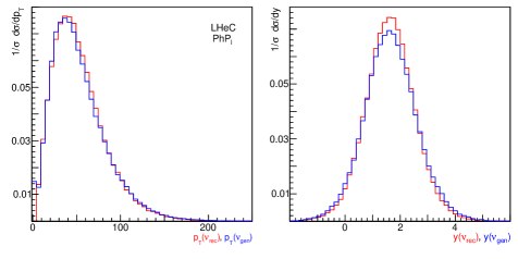
Figure 15: Normalized differential cross sections with respect to transverse momentum and rapidity for the reconstructed neutrino (red line) and the generated one (blue line).

We assess the goodness of our approach to neutrino reconstruction by comparing the transverse momentum and the rapidity of the generated neutrino and the reconstructed one. Here the generated neutrino is identified by requiring it to be a decay product of a $W$ boson which, in turn, is a decay product of a top quark. Notice that this is not a full validation, since the two distributions need not be identical, but we expect them to be close to each other. The result of this comparison is shown in figure 15. The transverse-momentum distributions are seen in the figure to be essentially equal, as expected, and the rapidity distributions are very close to each other, with the reconstructed neutrino distribution being slightly narrower, and therefore slightly taller at the maximum.

Appendix B Allowed ($\kappa$,$\widetilde{\kappa}$) region from ${\overline{B}}\to X_{s}\gamma$ branching ratio and $CP$ asymmetry.

In this appendix we obtain bounds on $\kappa$ and $\widetilde{\kappa}$ from a comparison of the experimental and theoretical values of the ${\overline{B}}\to X_{s}\gamma$ branching ratio and $CP$ asymmetry.

B.1 Scale dependence of $C^{33}_{uB}$ and $\kappa$, $\tilde{\kappa}$.

Before entering into the discussion of ${\rm BR}({\overline{B}}\to X_{s}\gamma)$ let us consider the scale dependence of the effective coefficients. The contribution of $\kappa$ (and $\tilde{\kappa}$) to the effective coefficient $C_{7}$ is taken (as usual) at the scale $m_{W}$ ($\kappa(m_{W})$ or $C^{33}_{uB}(m_{W})$) and this is denoted by $\Delta C_{7}(m_{W})$. On the other hand, the limits from $t\overline{t}$ photoproduction are to be considered at the $m_{t}$ scale ($\kappa(m_{t})$ or $C^{33}_{uB}(m_{t})$). These two scales are not too far apart and the running produces only a few percent change in numerical value. The RGE for the running of $C^{33}_{uB}$, (and indeed also for all of the other dimension-six effective operators) has been provided in References [53] and [54]:

$$16\pi^{2}\mu\frac{d}{d\mu}C^{33}_{uB} = \left(\frac{15}{2}y^{2}_{t}+\frac{8}{3}g^{2}_{s}-\frac{9}{4}g^{2}+(8+25/36){g^{\prime}}^{2}\right)C^{33}_{uB}\;,$$

$${\rm so}\;{\rm that}\;\;\;\;\mu\frac{d}{d\mu}C^{33}_{uB} \simeq 0.073C^{33}_{uB}\;,$$

$${\rm and}\;{\rm then}\;\;\;\;C^{33}_{uB}(m_{t}) \simeq 1.06\;C^{33}_{uB}(m_{W})\;,$$ (41)

where in the above equations some approximations have been made. The only Yukawa factor considered is the top’s $y_{t}=1$, and the values of the gauge couplings have been taken as nearly constant and at the scale $m_{Z}$. Also, in general there are contributions from other dimension-six operators, but we are not considering them. In the context of a global analysis with several effective operators and a variety of observables, keeping track of the scale dependence is important because mixing effects can be significant. However we do not expect, even in a general context, that there will be a substantial variation of $C^{33}_{uB}$ in going from the scale $m_{t}$ down to $m_{W}$. A variation of a few percent given by the factor $1.06$ is small but we will take it into account.

B.2 The branching ratio $BR({\overline{B}}\to X_{s}\gamma)$

So now let us turn our attention to ${\overline{B}}\to X_{s}\gamma$. The ${\overline{B}}\to X_{s}\gamma$ branching ratio and associated $CP$ asymmetry are known to be very good indirect tests of the anomalous electromagnetic dipole moments of the top quark as well as many other NP scenarios (See for instance: [22], [16], [55], [56], [25]). A recent study that uses $BR({\overline{B}}\to X_{s}\gamma)$ can be found in [23], and we will use the same average measurement by [57] that they used:

$$10^{4}BR({\overline{B}}\to X_{s}\gamma)^{\rm exp}_{E\gamma>1.6{\rm GeV}}=3.32\pm 0.15\;,$$ (42)

and the same NNLO SM calculation [58] (also [59, 60]):

$$10^{4}BR({\overline{B}}\to X_{s}\gamma)^{\rm SM}_{E\gamma>1.6{\rm GeV}}=3.36\pm 0.23\;.$$ (43)

The allowed ($\kappa,{\widetilde{\kappa}}$) parameter regions obtained below are based on these two values.

The ${\overline{B}}\to X_{s}\gamma$ branching fraction is given by [61]:

$$BR({\overline{B}}\to X_{s}\gamma)^{\rm th}_{E\gamma>E_{0}}=BR({\overline{B}}\to X_{c}e\overline{\nu})_{\rm exp}\frac{|V^{*}_{ts}V_{tb}|}{|V_{cb}|}\frac{6\alpha_{e}}{\pi C}\left(P(E_{0})+N(E_{0})\right)\;,$$ (44)

where $E_{0}=1.6$GeV is the minimum photon energy, $P(E_{0})$ and $N(E_{0})$ are the perturbative and nonperturbative contributions. The constant $C$ is a ratio of ${\overline{B}}\to X_{c}e\overline{\nu}$ and ${\overline{B}}\to X_{u}e\overline{\nu}$ amplitudes times CKM parameters and it has an experimental value of $0.568$ [62]. The perturbative term is a polynomial in the effective Wilson coefficients of the effective Hamiltonian at the scale $\mu_{b}$ [23, 61]:

$$P(E_{0})=\sum^{8}_{i,j=1}C_{i}^{\rm eff}(\mu_{b})C_{j}^{\rm eff}(\mu_{b})K_{ij}(E_{0},\mu_{b})\;,$$ (45)

with the Wilson coefficients expanded as:

$$C_{i}^{\rm eff}(\mu_{b})=C_{j}^{(0)}(\mu_{b})+\frac{\alpha_{s}(\mu_{b})}{4\pi}C_{j}^{(1)}(\mu_{b})+\left(\frac{\alpha_{s}(\mu_{b})}{4\pi}\right)^{2}C_{j}^{(2)}(\mu_{b})+\cdots~{},$$ (46)

where we have omitted electromagnetic correction terms [63]. In particular, for the coefficient $C_{7}^{(0)}$ [63]:

$$C_{7}^{(0)}(\mu_{b})=\eta^{16/23}C_{7}^{(0)}(m_{W})+\frac{8}{3}(\eta^{14/23}-\eta^{16/23})C_{8}^{(0)}(m_{W})+\cdots~{},$$ (47)

where $C^{(0)}_{7}(m_{W})$ is the LO contribution that comes from the dimension-four SM Lagrangian as well as the dimension-six operators of the SMEFT.

We will not attempt to use the lengthy expresions that arise when using eqs. (44)–(47). Instead, we will use a simplified expresion that was given many years ago in Ref. [63] (specifically, their eq. (20)). Let us separate SM and NP contributions $C_{7}=C^{\rm SM}_{7}+\Delta C^{NP}_{7}$; then, we have

$$10^{4}BR({\overline{B}}\to X_{s}\gamma)^{\rm th}_{E\gamma>E_{0}} = 10^{4}BR({\overline{B}}\to X_{s}\gamma)^{\rm SM}_{E\gamma>E_{0}}$$ (48)

$$+ B_{77}\frac{|\Delta C_{7}|^{2}}{|C_{7}^{\rm SM}|^{2}}+(2B_{77}+B_{27}+B_{78})Re\left[\frac{\Delta C_{7}}{C_{7}^{\rm SM}}\right]~{},$$

where the numbers $B_{ij}=B_{ij}(\mu,\delta)$ are given in [63]. For $\mu=m_{b}$, and $\delta=0.3$ ($E_{0}=(1-\delta)E^{\rm max}_{\gamma}=1.6$ GeV, $E^{\rm max}_{\gamma}=m_{b}/2$) we have $B_{77}=0.361$, $B_{27}=1.387$ and $B_{78}=0.08$. We therefore have (with $C_{7}^{\rm SM}(m_{W})=-0.22$ at NLO):

$$10^{4}BR(B\to X_{s}\gamma)^{\rm th}_{E\gamma>1.6\rm GeV} = 10^{4}BR(B\to X_{s}\gamma)^{\rm SM}_{E\gamma>1.6\rm GeV}$$ (49)

$$+ 7.4|\Delta C_{7}(m_{W})|^{2}-9.9Re\left[\Delta C_{7}(m_{W})\right]~{}.$$

The contribution from the dipole operator $Q_{tB}$ ($=Q_{uB}^{33}$ as defined in [26]) enters through the electromagnetic dipole vertex in the penguin diagram. Even before the top quark was observed a calculation was done in Ref. [24]. Their result was that at the scale $\mu=m_{W}$ (with $x=m_{t}^{2}/m^{2}_{W}$):

$$\Delta C_{7}(m_{W}) = \kappa G_{1}+i{\widetilde{\kappa}}G_{2}$$ (50)

$$= \sqrt{2}\frac{m_{t}}{m_{W}}\frac{v^{2}}{\Lambda^{2}}\frac{c_{w}}{s_{w}}\left[C_{tB}\frac{G_{1}+G_{2}}{2}+C^{*}_{tB}\frac{G_{1}-G_{2}}{2}\right]~{},$$

$$\frac{G_{1}+G_{2}}{2} = -\frac{1}{4}+\frac{1}{4}\frac{1}{x-1}+\frac{1}{8}\frac{x^{2}+x}{(x-1)^{2}}-\frac{1}{4}\frac{3x-2}{(x-1)^{3}}\ln{x}~{},$$

$$\frac{G_{1}-G_{2}}{2} = \frac{1}{8}-\frac{3}{8}\frac{1}{x-1}+\frac{1}{4}\frac{1}{(x-1)^{2}}+\frac{1}{4}\frac{x-2}{(x-1)^{3}}\ln{x}~{}.$$

This result is to be compared with the more recent one in [25] (scale $\mu_{W}=m_{W}$):

$$\Delta C_{7}(m_{W}) = \sqrt{2}\frac{m_{t}}{m_{W}}\frac{v^{2}}{\Lambda^{2}}\frac{c_{w}}{s_{w}}\left[C_{tB}E^{uB}_{7}+C^{*}_{tB}F^{uB}_{7}\right]~{},$$ (51)

$$E^{uB}_{7} = -\frac{1}{16}\frac{(x+1)^{2}}{(x-1)^{2}}-\frac{1}{8}\frac{x-3}{(x-1)^{3}}x^{2}\ln{x}~{},$$

$$F^{uB}_{7} = -\frac{1}{8}~{}.$$

We point out that these results from [25] are the ones that have been used in the literature in the last six years, as in [23]. The expressions (50) and (51) are noticeably different both in their analytical expressions and numerical values. For instance, with $m_{t}=174$GeV we have

$$\frac{G_{1}+G_{2}}{2} = -0.030\;,\;\;\;\frac{G_{1}-G_{2}}{2}=0.062$$

$$E^{uB}_{7} = -0.183\;,\;\;\;\;\;\;\;\;\;F^{uB}_{7}=-\frac{1}{8}\;,$$

which means that the results from [25] make the branching fraction much more sensitive to $C_{tB}$ (or $\kappa$) than those from [24]. It is beyond the scope of this work to revise these one-loop calculations in this case, though we may address this issue in some future study. For the present analysis, however, we will use both results. In terms of $\kappa$ and $\widetilde{\kappa}$, for $m_{t}=174$GeV we have:

$$\cite[cite]{[\@@bibref{}{hewett}{}{}]}\Delta C_{7}(m_{W}) = 0.032\kappa-i0.092{\widetilde{\kappa}}~{},$$ (52)

$$\cite[cite]{[\@@bibref{}{crivellin15}{}{}]}\Delta C_{7}(m_{W}) = -0.416\kappa-i0.166{\widetilde{\kappa}}~{}.$$ (53)

Inserting the recent SM value of $a^{\rm SM}=3.36$ and either eq. (52) or eq. (53) into eq. (49), we obtain:

$$10^{4}BR(B\to X_{s}\gamma)^{\rm theo}=3.36\pm 0.23+BR_{\kappa,\widetilde{\kappa}}~{},$$ (54)

with

$$\cite[cite]{[\@@bibref{}{hewett}{}{}]}BR_{\kappa,\widetilde{\kappa}} = -0.32\kappa+0.01\kappa^{2}+0.06{\widetilde{\kappa}}^{2}~{},$$ (55)

$$\cite[cite]{[\@@bibref{}{crivellin15}{}{}]}BR_{\kappa,\widetilde{\kappa}} = 4.1\kappa+1.3\kappa^{2}+0.2{\widetilde{\kappa}}^{2}~{}.$$ (56)

Before writing down the formulas for the allowed parameter region, we would like to point out that as we were aware of the recent study of constraints on $C_{tB}$ from $t{\overline{t}}\gamma$ and $B\to X_{s}\gamma$ in [23], we made a comparison of our results with theirs. We first notice that they use the NP contribution $\Delta C_{7}$ by [25] (they define a coefficient ${\tilde{C}}_{uB}$ that is equal to $\kappa/5.62$), which is written in our eq. (53). Then, they plot the dependence of ${\rm BR}(B\to X_{s}\gamma)$ on ${\tilde{C}}_{uB}$ which has the shape of a parabola. We have compared the ${\rm BR}(B\to X_{s}\gamma)$ we obtain by using eq. (49) with their plot and we have found good agreement.

The difference between the SM and the experimental values is $3.36-3.32=0.04$ with an uncertainty given by $\sqrt{0.15^{2}+0.23^{2}}=0.28$. We can then set, at the $1\sigma$ C.L.:

$$-0.04-0.28\leq BR_{\kappa,\widetilde{\kappa}}\leq-0.04+0.28\;.$$ (57)

Thus, by setting ${\widetilde{\kappa}}=0$ we get from $B\to X_{s}\gamma$:

$$\cite[cite]{[\@@bibref{}{hewett}{}{}]}: \qquad-0.75\leq{\kappa}\leq 1.0~{},$$ (58)

$$\cite[cite]{[\@@bibref{}{crivellin15}{}{}]}: \qquad-0.08\leq{\kappa}\leq 0.06~{},$$ (59)

which are the individual-coupling limits on $\kappa$ from the branching ratio $BR({\overline{B}}\to X_{s}\gamma)$.

The above limits for $\kappa$ are set at the scale $m_{W}$. We can now obtain the corresponding limits at the scale $m_{t}$. To do so, we just use equation (41): $\kappa(m_{t})=1.06\kappa(m_{W})$. Let us rewrite equations (55) and (56) at the scale $m_{t}$ (define $k_{t}\equiv\kappa(m_{t})$):

$$\cite[cite]{[\@@bibref{}{hewett}{}{}]}BR_{\kappa_{t},\widetilde{\kappa}_{t}} = -0.302\kappa_{t}+0.009\kappa_{t}^{2}+0.053{\widetilde{\kappa}_{t}}^{2}~{},$$ (60)

$$\cite[cite]{[\@@bibref{}{crivellin15}{}{}]}BR_{\kappa_{t},\widetilde{\kappa}_{t}} = 3.87\kappa_{t}+1.16\kappa_{t}^{2}+0.178{\widetilde{\kappa}_{t}}^{2}~{}.$$ (61)

Thus, by setting ${\widetilde{\kappa}_{t}}=0$ we get:

$$\cite[cite]{[\@@bibref{}{hewett}{}{}]}: \qquad-0.78\leq{\kappa_{t}}\leq 1.10~{},$$ (62)

$$\cite[cite]{[\@@bibref{}{crivellin15}{}{}]}: \qquad-0.085\leq{\kappa_{t}}\leq 0.064~{},$$ (63)

B.3 The $CP$ asymmetry ${\cal A}_{Xs\gamma}$.

The expression for the $B\to X_{s}\gamma$ $CP$ asymmetry can be written as [64]:

$${\cal A}_{Xs\gamma} = \left[\;\left(\frac{40}{81}-\frac{40}{9}\frac{\Lambda_{c}}{m_{b}}\right)\alpha_{s}+\pi\frac{\Lambda^{c}_{17}}{m_{b}}\;\right]\;{\rm Im}\frac{C_{1}}{C_{7}}$$ (64)

$$- \left(\frac{4}{9}\alpha_{s}+\frac{4}{3}\pi^{2}\alpha_{s}\frac{\Lambda_{78}}{m_{b}}\right)\;{\rm Im}\frac{C_{8}}{C_{7}}$$

$$- \left(\alpha_{s}\frac{40}{9}\frac{\Lambda_{c}}{m_{b}}+\pi\frac{\Lambda^{u}_{17}-\Lambda^{c}_{17}}{m_{b}}\right)\;{\rm Im}\left(\epsilon_{s}\frac{C_{1}}{C_{7}}\right)\,,$$

where the coefficients $C_{j}$ and $\alpha_{s}(\mu)=0.3$ at the scale $\mu=2$ GeV are given by [64]:

$$C_{1}(\mu)=1.204\;,\;\;C_{8}(\mu)=-0.175\;,\;\;C_{7}(\mu)=-0.381+0.55\Delta C_{7}(m_{W})\;,$$ (65)

with $\Delta C_{7}$ given in (52), (53), and where $0.55=\eta^{16/23}$ is the factor for the running from the $m_{W}$ scale down to $\mu=2$GeV [63]. In addition $\Lambda_{c}\simeq 0.38$ GeV, $m_{b}=4.6$; and $\epsilon_{s}$, by using the Wolfenstein parameters in [64], is given by:

$$\epsilon_{s}=\frac{V_{ub}V^{*}_{us}}{V_{tb}V^{*}_{td}}=10^{-2}\left(-0.8+i1.8\right)\;.$$ (66)

The $\Lambda$ parameters are not known and in [64] they were given some limits that have recently been revised. The parameter with the greatest uncertainty is $\Lambda^{u}_{17}$: $-660<\Lambda^{u}_{17}<660$ MeV [65]. The other parameters have an allowed range smaller by two orders of magnitude: $-7<\Lambda^{c}_{17}<10$ MeV and $17<\Lambda_{78}<190$ MeV [65].

We can now write ${\cal A}_{Xs\gamma}$ in (64) with the numerical values in [64]:

$$10^{2}{\cal A}_{Xs\gamma} = \left(6.91\times 10^{-2}+3.8x_{c}+0.7x_{78}\right)\;{\rm Im}\left[\frac{1}{C_{7}}\right]$$ (67)

$$+ \left(0.133+3.78x_{uc}\right)\;{\rm Im}\left[\frac{-\epsilon_{s}}{C_{7}}\right]\;,$$

$$x_{u} = \frac{\Lambda^{u}_{17}}{m_{b}}\;,\;\;x_{c}=\frac{\Lambda^{c}_{17}}{m_{b}}\;,\;\;x_{uc}=x_{u}-x_{c}\;,\;\;x_{78}=\frac{\Lambda_{78}}{m_{b}}$$

As we have two different values for $\Delta C_{7}$, will obtain two different evaluations of the asymmetry:

$$\cite[cite]{[\@@bibref{}{hewett}{}{}]}10^{2}{\cal A}_{Xs\gamma} =|C_{7}|^{-2}\left(0.091+0.355{\widetilde{\kappa}}-0.004\kappa\right)\;,$$ (68)

$$|C_{7}|^{2} =10^{-2}\left[(3.81-0.176\kappa)^{2}+0.256{\widetilde{\kappa}}^{2}\right]\;,$$

and

$$\cite[cite]{[\@@bibref{}{crivellin15}{}{}]}10^{2}{\cal A}_{Xs\gamma} =|C_{7}|^{-2}\left(0.091+0.64{\widetilde{\kappa}}+0.055\kappa\right)\;,$$ (69)

$$|C_{7}|^{2} =10^{-2}\left[(3.81+2.29\kappa)^{2}+0.834{\widetilde{\kappa}}^{2}\right]\;.$$

In both cases, (68) and (69), by setting $\kappa={\widetilde{\kappa}}=0$ we obtain $10^{2}{\cal A}^{\rm SM}_{Xs\gamma}=0.627$. There is an estimated $\pm 2.6$ theoretical uncertainty in $10^{2}{\cal A}_{Xs\gamma}$ that comes from $\Lambda^{u}_{17}$. The experimental averaged value for the asymmetry can be found in [51]: $10^{2}{\cal A}^{\rm exp}_{Xs\gamma}=1.5\pm 1.1$. After adding the two uncertainties in quadrature we obtain a global, ($1\sigma$) 68% C.L., $\pm 2.8$ uncertainty and we can write the inequality:

$$-2.8+1.5\leq 10^{2}{\cal A}_{Xs\gamma}\leq 2.8+1.5$$ (70)

In order to find the individual limits on $\widetilde{\kappa}$ from both values of $C_{7}$ we set $\kappa=0$ and approximate $|C_{7}|^{2}\simeq 0.381^{2}$ in (68), (69) to obtain:

$$\cite[cite]{[\@@bibref{}{hewett}{}{}]}: \qquad-0.79\leq{\widetilde{\kappa}}\leq 1.5$$ (71)

$$\cite[cite]{[\@@bibref{}{crivellin15}{}{}]}: \qquad-0.44\leq{\widetilde{\kappa}}\leq 0.83$$

As before, let us now remember that so far the coupling $\kappa$ has been set at the scale $m_{W}$. Replacing $\kappa$ by $\kappa_{t}/1.06$ in eqs. (68)-(69), we obtain:

$$\cite[cite]{[\@@bibref{}{hewett}{}{}]}10^{2}{\cal A}_{Xs\gamma} =|C_{7}|^{-2}\left(0.091+0.335{\widetilde{\kappa}_{t}}-0.0038\kappa_{t}\right)\;,$$ (72)

$$|C_{7}|^{2} =10^{-2}\left[(3.81-0.166\kappa_{t})^{2}+0.228{\widetilde{\kappa}_{t}}^{2}\right]\;,$$

and

$$\cite[cite]{[\@@bibref{}{crivellin15}{}{}]}10^{2}{\cal A}_{Xs\gamma} =|C_{7}|^{-2}\left(0.091+0.604{\widetilde{\kappa}_{t}}+0.052\kappa_{t}\right)\;,$$ (73)

$$|C_{7}|^{2} =10^{-2}\left[(3.81+2.160\kappa_{t})^{2}+0.742{\widetilde{\kappa}_{t}}^{2}\right]\;.$$

From these equations, by setting $\kappa_{t}=0$ we obtain the bounds,

$$\cite[cite]{[\@@bibref{}{hewett}{}{}]}: \qquad-0.84\leq{\widetilde{\kappa}_{t}}\leq 1.67$$ (74)

$$\cite[cite]{[\@@bibref{}{crivellin15}{}{}]}: \qquad-0.47\leq{\widetilde{\kappa}_{t}}\leq 0.93$$ (75)

We point out that in Ref. [55] limits on $\widetilde{\kappa}$ that are three orders of magnitude stronger have been reported:

$$|{\widetilde{\kappa}}|\leq 1.4\times 10^{-3}~{},$$ (76)

based on nuclei and electron electric-dipole moment measurements.

Appendix C Single-coupling bounds for Wilson coefficients

In this appendix we write the most relevant results from tables 4–8 for the couplings $\widetilde{C}_{\varphi q}^{(-)33}\rule{0.0pt}{12.0pt}$, $\widetilde{C}_{uB}^{33}\rule{0.0pt}{12.0pt}$ associated with the basis operators $\mathcal{O}^{33}_{uB}$, $\mathcal{O}_{\varphi q}^{(-)33}$ in terms of the couplings $C_{uB}^{33}\rule{0.0pt}{12.0pt}$, $C_{\varphi q}^{(-)33}\rule{0.0pt}{12.0pt}$ associated with $Q^{33}_{uB}$, $Q_{\varphi q}^{(-)33}$. Doing so is useful to compare with some results in the literature. From those tables and (4) we obtain the limits on Wilson coefficients given below at the LHeC energy. Results for the FCC-he energy are completely analogous, as seen from the tables in sections 6.2, 6.3.

The limits on $C_{\varphi q}^{(-)33}\rule{0.0pt}{12.0pt}$ are,

	$C_{\varphi q}^{(-)33}\rule{0.0pt}{12.0pt}$, LHeC, $PhP_{III}$
$\varepsilon_{\mathrm{exp}}$	68% C.L.	95% C.L.
12%	-0.58,0.64	-1.10,1.37
15%	-0.71,0.81	-1.37,1.81
18%	-0.86,0.99	-1.62,2.31

The limits on $\widetilde{C}_{uB}^{33}\rule{0.0pt}{12.0pt}$ are,

	$C_{uB\,r}^{33}\rule{0.0pt}{12.0pt}$, LHeC, $PhP_{I}$		$C_{uB\,i}^{33}\rule{0.0pt}{12.0pt}$, LHeC, $PhP_{I}$
$\varepsilon_{\mathrm{exp}}$	68% C.L.	95% C.L.	68% C.L.	95% C.L.
12%	-0.24,0.29	-0.45,0.65	$\pm$0.89	$\pm$1.24
15%	-0.30,0.37	-0.54,1.00	$\pm$0.94	$\pm$1.36
18%	-0.35,0.46	-0.65,3.54	$\pm$1.06	$\pm$1.48

These values are to be compared, e.g., with table 1 and with [16].

References

- [1] P. Agostini et al. [LHeC and FCC-he Study Group], “The Large Hadron-Electron Collider at the HL-LHC,” J. Phys. G 48 (2021) 110501. [arXiv:2007.14491 [hep-ex]].
- [2] Q. H. Cao, B. Yan, C. P. Yuan and Y. Zhang, “Probing couplings using boson polarization in production at hadron colliders,” Phys. Rev. D 102, 055010 (2020) [arXiv:2004.02031 [hep-ph]].
- [3] J. Montaño, H. Novales-Sánchez and J. J. Toscano, “Effects of universal extra dimensions on top-quark electromagnetic interactions,” J. Phys. G 47, 015002 (2020) [arXiv:1908.06226 [hep-ph]].
- [4] R. Martinez and G. Valencia, “Top and bottom tensor couplings from a color octet scalar,” Phys. Rev. D 95, 035041 (2017) [arXiv:1612.00561 [hep-ph]].
- [5] L. Han, Y. J. Zhang and Y. B. Liu, “Single vector-like -quark search via the decay channel at the LHeC,” Phys. Lett. B 771, 106-112 (2017)
- [6] Y. J. Zhang, L. Han and Y. B. Liu, “Single production of the top partner in the channel at the LHeC,” Phys. Lett. B 768, 241-247 (2017)
- [7] S. Fayazbakhsh, S. T. Monfared and M. Mohammadi Najafabadi, “Top Quark Anomalous Electromagnetic Couplings in Photon-Photon Scattering at the LHC,” Phys. Rev. D 92, 014006 (2015) [arXiv:1504.06695 [hep-ph]].
- [8] I. V. Truten and A. Y. Korchin, “The top-quark polarization beyond the Standard Model in electron–positron annihilation,” Int. J. Mod. Phys. A 34, 1950067 (2019) [arXiv:1902.09911 [hep-ph]].
- [9] S. M. Etesami, S. Khatibi and M. Mohammadi Najafabadi, “Study of top quark dipole interactions in production associated with two heavy gauge bosons at the LHC,” Phys. Rev. D 97, 075023 (2018) [arXiv:1712.07184 [hep-ph]].
- [10] H. Denizli, A. Senol, A. Yilmaz, I. Turk Cakir, H. Karadeniz and O. Cakir, “Top quark FCNC couplings at future circular hadron electron colliders,” Phys. Rev. D 96, 015024 (2017) [arXiv:1701.06932 [hep-ph]].
- [11] K. Fuyuto and M. Ramsey-Musolf, “Top Down Electroweak Dipole Operators,” Phys. Lett. B 781, 492-498 (2018) [arXiv:1706.08548 [hep-ph]].
- [12] M. Fael and T. Gehrmann, “Probing top quark electromagnetic dipole moments in single-top-plus-photon production,” Phys. Rev. D 88, 033003 (2013) [arXiv:1307.1349 [hep-ph]].
- [13] A. Kozachuk and D. Melikhov, “Constraints on the anomalous couplings from -physics experiments,” Symmetry 12, 1506 (2020) [arXiv:2004.13127 [hep-ph]].
- [14] I. A. Sarmiento-Alvarado, Antonio O. Bouzas, F. Larios, “Analysis of top-quark charged-current coupling at the LHeC,” J. Phys. G 42 (2015) 085001 [arXiv:1412.6679 [hep-ph]].
- [15] S. Dutta, A. Goyal, M. Kumar and B. Mellado, “Measuring anomalous couplings at collider,” Eur. Phys. J. C 75, 577 (2015) [arXiv:1307.1688 [hep-ph]].
- [16] A. Bouzas, F. Larios, “Probing and couplings at the LHeC,” Phys. Rev. D 88 (2013) 094007 [arXiv:1308.5634 [hep-ph]].
- [17] A. A. Billur, M. Köksal and A. Gutiérrez-Rodríguez, “Improved sensitivity on the electromagnetic dipole moments of the top quark in , and collisions at the CLIC,” Phys. Rev. D 96, 056007 (2017) [arXiv:1702.03708 [hep-ph]].
- [18] A. A. Billur, M. Köksal, A. Gutiérrez-Rodrıguez and M. A. Hernández-Ruız, “Projections for model-independent limit estimates on top-quark anomalous electromagnetic couplings at the FCC-he,” Eur. Phys. J. Plus 134, 547 (2019) [arXiv:1811.10462 [hep-ph]].
- [19] M. A. Hernández-Ruíz, A. Gutiérrez-Rodríguez, M. Köksal and A. A. Billur, “FCC-he sensitivity estimates on the anomalous electromagnetic dipole moments of the top-quark,” Nucl. Phys. B 941, 646-664 (2019) [arXiv:1812.08971 [hep-ph]].
- [20] M. Köksal, A. A. Billur, A. Gutiérrez-Rodríguez and M. A. Hernández-Ruíz, “Sensitivity measuring expected on the electromagnetic anomalous couplings in the vertex at the FCC-he,” Int. J. Mod. Phys. A 35, 2050178 (2020) [arXiv:1905.02564 [hep-ph]].
- [21] V. M. Budnev, I. F. Ginzburg, G. V. Meledin, V. G. Serbo, “The Two-Photon Particle Production Mechanism. Physical Problems. Applications. Equivalent Photon Approximation,” Phys. Rep. 15 (1975) 181.
- [22] A. Bouzas, F. Larios, “Electromagnetic dipole moments of the top quark,” Phys. Rev. D 87 (2013) 074015 [arXiv:1212.6575 [hep-ph]].
- [23] S. Bismann, J. Erdmann, C. Grunwald, G. Hiller and K. Kröninger, “Constraining top-quark couplings combining top-quark and decay observables,” Eur. Phys. J. C 80, 136 (2020) [arXiv:1909.13632 [hep-ph]].
- [24] J. L. Hewett and T. G. Rizzo, “Using to probe top quark couplings,” Phys. Rev. D 49 (1994) 319 [arXiv:hep-ph/9305223 [hep-ph]].
- [25] J. Aebischer, A. Crivellin, M. Fael and C. Greub, “Matching of gauge invariant dimension-six operators for and transitions,” JHEP 05, 037 (2016), [arXiv:1512.02830 [hep-ph]].
- [26] B. Grzadkowski, M. Iskrzyński, M. Misiak, J. Rosiek, “Dimension-Six Terms in the Standard Model Lagrangian,” JHEP 10 (2010) 085 [arXiv:1008.4884 [hep-ph]].
- [27] C. Zhang, “Effective field theory approach to top-quark decay at next-to-leading order in QCD,” Phys. Rev. D 90 (2014) 014008 [arXiv:1404.1264 [hep-ph]].
- [28] E. E. Jenkins, A. V. Manohar and M. Trott, “Naive Dimensional Analysis Counting of Gauge Theory Amplitudes and Anomalous Dimensions,” Phys. Lett. B 726, 697-702 (2013) [arXiv:1309.0819 [hep-ph]].
- [29] ATLAS collaboration, “Measurement of the boson polarization in top quark decays with the ATLAS detector,” JHEP 06 (2012) 088 [arXiv:1205.2484].
- [30] CMS collaboration, “Measurement of the boson helicity in top-quark decays from production in lepton+jets events in collisions at TeV,” JHEP 10 (2013) 167 [arXiv:1308.3879].
- [31] CMS collaboration, “Measurement of the boson helicity in events with a single reconstructed top quark in collisions at TeV,” JHEP 01 (2015) 053 [arXiv:1410.1154].
- [32] CMS collaboration, “Search for anomalous couplings and flavour-changing neutral currents in -channel single top quark production in pp collisions at = 7 and 8 TeV,” JHEP 02 (2017) 028
- [33] J. J. Ethier, G. Magni, F. Maltoni, L. Mantani, E. R. Nocera, J. Rojo, E. Slade, E. Vryonidou and C. Zhang, “Combined SMEFT interpretation of Higgs, diboson, and top quark data from the LHC,” [arXiv:2105.00006 [hep-ph]].
- [34] B. Yan, Z. Yu and C. P. Yuan, “The anomalous couplings at the HERA and EIC,” Phys. Lett. B 822, 136697 (2021) [arXiv:2107.02134 [hep-ph]].
- [35] B. Yan and C. P. Yuan, “Anomalous Couplings: From LEP to LHC,” Phys. Rev. Lett. 127, 051801 (2021) [arXiv:2101.06261 [hep-ph]].
- [36] J. A. Aguilar Saavedra et al., “Interpreting top-quark LHC measurements in the standard-model effective field theory,” CERN report CERN-LPCC-2018-01 (2018) [arXiv:1802.07237 [hep-ph]]
- [37] S. Brown, A. Buckley, C. Englert, J. Ferrando, P. Galler, D. Miller, C. Wanotayaroj, N. Warrack and C. White, “New results from TopFitter,” PoS ICHEP2020, 322 (2021).
- [38] J. Ellis, M. Madigan, K. Mimasu, V. Sanz and T. You, “Top, Higgs, Diboson and Electroweak Fit to the Standard Model Effective Field Theory,” JHEP 04, 279 (2021) [arXiv:2012.02779 [hep-ph]].
- [39] V. Miralles, M. M. López, M. M. Llácer, A. Peñuelas, M. Perelló and M. Vos, “The top quark electro-weak couplings after LHC Run 2,” [arXiv:2107.13917 [hep-ph]].
- [40] S. Bismann, C. Grunwald, G. Hiller and K. Kröninger, “Top and Beauty synergies in SMEFT-fits at present and future colliders,” JHEP 06, 010 (2021) [arXiv:2012.10456 [hep-ph]].
- [41] W. Bernreuther, L. Chen, I. García, M. Perelló, R. Poeschl, F. Richard, E. Ros and M. Vos, “CP-violating top quark couplings at future linear colliders,” Eur. Phys. J. C 78, 155 (2018) [arXiv:1710.06737 [hep-ex]].
- [42] U. Baur, A. Juste, L. H. Orr and D. Rainwater, “Probing electroweak top quark couplings at hadron colliders,” Phys. Rev. D 71, 054013 (2005) [arXiv:hep-ph/0412021 [hep-ph]].
- [43] U. Baur, A. Juste, D. Rainwater and L. H. Orr, “Improved measurement of couplings at the CERN LHC,” Phys. Rev. D 73, 034016 (2006) [arXiv:hep-ph/0512262 [hep-ph]].
- [44] ATLAS collaboration, “Prospects for the measurement of with the upgraded ATLAS detector at the High-Luminosity LHC,” CERN report ATL-PHYS-PUB-2018-049, Dec. 2018.
- [45] J. Alwall, R. Frederix, S. Frixione, V. Hirschi, F. Maltoni, O. Mattelaer, H.-S. Shao, T. Stelzer, P. Torrielli, M. Zaro, “The automated computation of tree-level and next-to-leading order differential cross sections, and their matching to parton shower simulations,” J. High Energy Phys. 07 (2014) 079 [arXiv:1405.0301 [hep-ph]].
- [46] T. Sjostrand, S. Mrenna, P. Skands, “Pythia 6.4 Physics and Manual,” J. High Energy Phys. 05 (2006) 26 [arXiv:hep-ph/0603175].
- [47] J. de Favereau, C. Delaere, P. Demin, A. Giammanco, V. Lemaitre, A. Mertens, M. Selvaggi, “DELPHES 3: a modular framework for fast simulation of a generic collider experiment,” J. High Energy Phys. 02 (2014) 057 [arXiv:1307.6346 [hep-ph]].
- [48] M. Cacciari, G. P. Salam, G. Soyez, “FastJet User Manual,” Eur. Phys. J. C 72 (2012) 1896 [arXiv:1111.6097 [hep-ph]].
- [49] R. Brun, F. Rademakers, “ROOT — An object oriented data analysis framework,” Nucl. Instrum. Methods Phys. Res. A 389 (1997) 81.
- [50] J. L. Abelleira Fernández et al, “A Large Hadron Electron Collider at CERN report on the physics and design concepts for machine and detector,” J. Phys. G 39 2012 075001 [arXiv:1206.2913 [hep-ph]]
- [51] P. A. Zyla et al. (Particle Data Group), “Review of Particle Physics,” Prog. Theor. Exp. Phys. 2020 (2020) 083C01, and 2021 update.
- [52] A. Alloul, N. D. Christensen, C. Degrande, C. Duhr, B. Fuks, “FeynRules 2.0 – A complete toolbox for tree-level phenomenology,” Comput. Phys. Commun. 185 (2014) 2250 [arXiv:1310.1921 [hep-ph]].
- [53] E. E. Jenkins, A. V. Manohar and M. Trott, “Renormalization Group Evolution of the Standard Model Dimension Six Operators II: Yukawa Dependence,” JHEP 01, 035 (2014) [arXiv:1310.4838 [hep-ph]].
- [54] R. Alonso, E. E. Jenkins, A. V. Manohar and M. Trott, “Renormalization Group Evolution of the Standard Model Dimension Six Operators III: Gauge Coupling Dependence and Phenomenology,” JHEP 04, 159 (2014) [arXiv:1312.2014 [hep-ph]].
- [55] V. Cirigliano, W. Dekens, J. de Vries and E. Mereghetti, “Constraining the top-Higgs sector of the Standard Model Effective Field Theory,” Phys. Rev. D 94 (2016) 034031 [arXiv:1605.04311 [hep-ph]].
- [56] A. G. Akeroyd, S. Moretti, T. Shindou and M. Song, “CP asymmetries of in models with three Higgs doublets,” Phys. Rev. D 103 (2021) 015035 [arXiv:2009.05779 [hep-ph]].
- [57] Y. S. Amhis et al. [HFLAV], “Averages of b-hadron, c-hadron, and -lepton properties as of 2018,” Eur. Phys. J. C 81 (2021) 226 [arXiv:1909.12524 [hep-ex]].
- [58] M. Misiak, H. M. Asatrian, R. Boughezal, M. Czakon, T. Ewerth, A. Ferroglia, P. Fiedler, P. Gambino, C. Greub and U. Haisch, et al. “Updated NNLO QCD predictions for the weak radiative B-meson decays,” Phys. Rev. Lett. 114 (2015) 221801 [arXiv:1503.01789 [hep-ph]].
- [59] M. Misiak, A. Rehman and M. Steinhauser, “Towards at the NNLO in QCD without interpolation in mc,” JHEP 06 (2020) 175 [arXiv:2002.01548 [hep-ph]].
- [60] M. Czakon, P. Fiedler, T. Huber, M. Misiak, T. Schutzmeier and M. Steinhauser, “The contribution to at ,” JHEP 04 (2015) 168 [arXiv:1503.01791 [hep-ph]].
- [61] M. Misiak and M. Steinhauser, “NNLO QCD corrections to the matrix elements using interpolation in m(c),” Nucl. Phys. B 764, 62-82 (2007) [arXiv:hep-ph/0609241 [hep-ph]].
- [62] A. Alberti, P. Gambino, K. J. Healey and S. Nandi, “Precision Determination of the Cabibbo-Kobayashi-Maskawa Element ,” Phys. Rev. Lett. 114, 061802 (2015) [arXiv:1411.6560 [hep-ph]].
- [63] A. L. Kagan and M. Neubert, “QCD anatomy of decays,” Eur. Phys. J. C 7 (1999) 5 [arXiv:hep-ph/9805303 [hep-ph]].
- [64] M. Benzke, S. J. Lee, M. Neubert and G. Paz, “Long-Distance Dominance of the CP Asymmetry in Decays,” Phys. Rev. Lett. 106 (2011) 141801 [arXiv:1012.3167 [hep-ph]].
- [65] A. Gunawardana and G. Paz, “Reevaluating uncertainties in decay,” JHEP 11 (2019) 141 [arXiv:1908.02812 [hep-ph]].