Geometric Quasilinearization Framework for Analysis and Design of Bound-Preserving Schemes

Abstract

Solutions to many partial differential equations satisfy certain bounds or constraints. For example, the density and pressure are positive for equations of fluid dynamics, and in the relativistic case the fluid velocity is upper bounded by the speed of light, etc. As widely realized, it is crucial to develop bound-preserving numerical methods that preserve such intrinsic constraints. Exploring provably bound-preserving schemes has attracted much attention and is actively studied in recent years. This is however still a challenging task for many systems especially those involving nonlinear constraints.

Based on some key insights from geometry, we systematically propose an innovative and general framework, referred to as geometric quasilinearization (GQL), which paves a new effective way for studying bound-preserving problems with nonlinear constraints. The essential idea of GQL is to equivalently transfer all nonlinear constraints into linear ones, through properly introducing some free auxiliary variables. We establish the fundamental principle and general theory of GQL via the geometric properties of convex regions, and propose three simple effective methods for constructing GQL. We apply the GQL approach to a variety of partial differential equations, and demonstrate its effectiveness and remarkable advantages for studying bound-preserving schemes, by diverse challenging examples and applications which cannot be easily handled by direct or traditional approaches.

65M08, 65M60, 65M12, 65M06, 35L65

1 Introduction

Solutions to many partial differential equations (PDEs) satisfy certain algebraic constraints, which are usually derived from some (physical) bound principles, for example, the positivity of density and pressure. Consider such time-dependent PDE systems in a general form

(1) $$\partial_{t}{\bf u}+\mathbfcal{L}({\bf u})={\bf 0},~{}~{}~{}\qquad{\bf u}({\bm{x}},0)={\bf u}_{0}({\bm{x}}),$$

where $\mathbfcal{L}$ denotes the differential operator associated with the spatial coordinates ${\bm{x}}$, and suppose the system Eq. 1 is defined in a bounded domain with suitable boundary conditions. An important class of such systems, which we are particularly interested in, are the hyperbolic conservation laws:

(2) $$\partial_{t}{\bf u}+\nabla\cdot{\bf f}({\bf u})={\bf 0},\qquad{\bf u}({\bm{x}},0)={\bf u}_{0}({\bm{x}}),$$

and other related hyperbolic or convection dominated equations.

Assume that the algebraic constraints (bound principles) can be expressed by either the positivity or the non-negativity of several (linear or nonlinear) functions of ${\bf u}$ as

(3) $$g_{i}({\bf u})>0~{}~{}\forall i\in\mathbb{I},\qquad g_{i}({\bf u})\geq 0~{}~{}\forall i\in\widehat{\mathbb{I}},$$

where $\mathbb{I}\cup\widehat{\mathbb{I}}=\{1,\dots,I\}$ with the positive integer $I$ denoting the total number of the constraints. In other words, the evolved variables ${\bf u}=(u_{1},\dots,u_{N})^{\top}$ belong to the admissible state set:

(4) $$G=\left\{{\bf u}\in\mathbb{R}^{N}:~{}g_{i}({\bf u})>0~{}~{}\forall i\in\mathbb{I},\quad g_{i}({\bf u})\geq 0~{}~{}\forall i\in\widehat{\mathbb{I}}\right\}.$$

Throughout this paper, we assume $G$ is convex, which is valid for many physical systems (several typical examples will be given in Section 2). It is worth noting that the functions $\{g_{i}({\bf u}),1\leq i\leq I\}$ are not necessarily concave (and not required to be concave in this paper). Moreover, we assume that $G$ is an invariant region for the exact solution of the system Eq. 1, namely,

• If ${\bf u}({\bm{x}},0)\in G$ for all $\bm{x}$, then ${\bf u}({\bm{x}},t)\in G$ for all ${\bm{x}}$ and $t>0$.

A basic goal behind the design of numerical methods solving Eq. 1 is that they can inherit as much as possible the intrinsic properties of the system Eq. 1. The constraints Eq. 3 and the associated invariant region $G$ carry important properties of the exact solution. It is natural and meaningful to explore bound-preserving schemes that keep the numerical solutions within the region $G$:

• If ${\bf u}_{h}(\cdot,t_{0})\in G$, then ${\bf u}_{h}(\cdot,t_{n})\in G$ for all $n\in\mathbb{N}$,

where ${\bf u}_{h}(\cdot,t_{n})$ denotes the numerical solutions at $n$th time level. In fact, preserving such constraints is not only necessary for physical significance, but also very crucial for theoretical analysis and numerical stability. If any of the intrinsic physical constraints Eq. 3 are violated numerically, the PDE system Eq. 1 and its discrete equations may become ill-posed outside the physical regimes. For example, when negative density and/or pressure are produced in numerically solving the compressible Euler equations, the key hyperbolicity of the system would be lost. As a result, failure to preserve such physically relevant constraints may cause serious numerical problems, for example, nonlinear instability, nonphysical solutions or phenomena, blowups of the code, etc. Therefore, it is significant and highly desirable to develop bound-preserving schemes.

In the past decades, the exploration of bound-preserving high-order numerical methods has attracted extensive attention and is actively studied, especially for hyperbolic and convection dominated equations (e.g. [40, 67, 68, 69, 71, 72, 63, 23, 51, 55]), and recently for some other types of time-dependent PDEs (e.g. [44, 8, 15, 25, 32]). For example, a general framework was established in [67, 68] for constructing bound-preserving high-order finite volume and discontinuous Galerkin schemes for scalar conservation laws and compressible Euler equations. A key step in this framework is to look for high-order schemes that have a provable “weak” bound-preserving property keeping the cell averages of the numerical solutions in the region $G$. Once such a property is proven, a simple scaling limiter can be used to enforce the constraints for the numerical solutions at any specified points [67, 68, 71]. The idea of this methodology has been applied to many other hyperbolic or convection dominated systems; see, for example, [60, 69, 9, 43, 10, 7, 41, 65, 66, 58, 24, 13, 59]. Another bound-preserving framework [63, 23, 33] is built on flux-correction limiters, which modify any high-order numerical fluxes to enforce the constraints by combining a provably bound-preserving (lower-order) numerical flux as the building block. This approach has also been applied to various physical systems (cf. [11, 12, 61, 56, 62, 50]). Recently, continuous finite element approximations with convex limiting were developed in [21, 22, 20] to preserve invariant regions for hyperbolic equations. Thorough reviews on bound-preserving efforts can be found in the survey articles [64, 45].

Yet, due to the lack of a general theory, how to rigorously analyze or prove whether a numerical scheme is genuinely bound-preserving remains a challenging task. Despite the success of the limiter-based frameworks (cf. [67, 68, 63, 23]) in constructing high-order bound-preserving schemes, the validity of those limiters is actually based on some (weak or lower-order) bound-preserving properties of the cell-average schemes and/or of the numerical fluxes as the key building blocks. Proving such properties is therefore necessary, but often very difficult [45, 51, 55]. To illustrate the challenges, we suppose that a numerical scheme for Eq. 1 may be written as

(5) $${\bf u}_{j}^{n+1}={\mathbfcal{E}}_{h}({\bf u}_{j-k}^{n},{\bf u}_{j-k+1}^{n},\dots,{\bf u}_{j}^{n},\dots\bf u_{j+s-1}^{n},{\bf u}_{j+s}^{n}),$$

where ${\mathbfcal{E}}_{h}$ is the discretization operator, the superscripts on $\bf u$ denote the time levels, and the subscripts on $\bf u$ indicate the indexes of the spatial grid or nodal points. The bound-preserving problem for the scheme Eq. 5 can boil down to answer

$$\mbox{ whether }~{}~{}{\bf u}_{j}^{n}\in G~{}~{}\forall j~{}~{}\mbox{ implies }~{}~{}{\bf u}_{j}^{n+1}\in G~{}~{}\forall j~{}?$$

In essence, it is to explore whether or not the range of the high-dimensional function ${\mathbfcal{E}}_{h}$ is always contained in $G$: ${\mathbfcal{E}}_{h}(G^{s+k+1})\subseteq G.$ For some scalar PDEs with linear constraints, for instance, the scalar conservation laws with the constraints linearly defined by maximum principle, a general approach for bound-preserving analysis and design is to exploit certain monotonicity in schemes; see, e.g., [67, 14, 31]. Yet, for PDE systems especially with nonlinear constraints, there is no unified tool like monotonicity, so that direct and complicated algebraic verification usually has to be performed for each constraint case-by-case for different schemes and different PDEs; see, e.g., [68, 38, 56, 41, 66, 35, 53]. Therefore, the design and analysis of bound-preserving schemes involving nonlinear constraints are highly nontrivial, even for first-order schemes; cf. [49, 2, 48, 39, 26, 34, 36, 57, 51].

Nonlinear constraints widely exist in many physical PDE systems; see several representative examples in Section 2. For instance, the physical constraints for solutions of the special relativistic magnetohydrodynamic (MHD) equations (25) include: the positivity of density $D$ and thermal pressure $p$, and the upper bound of fluid velocity field $\bm{v}$ by the speed of light $c$, namely,

(6) $$D>0,\qquad p({\bf u})>0,\qquad c-\|{\bm{v}}({\bf u})\|>0,$$

where the evolved variables ${\bf u}=(D,{\bm{m}},{\bf B},E)^{\top}$ with the momentum vector ${\bm{m}}\in\mathbb{R}^{3}$, the magnetic field ${\bf B}\in\mathbb{R}^{3}$, and the total energy $E$; see Example 2.7 and [55] for more details. The second and third constraints in Eq. 6 are highly nonlinear with respect to ${\bf u}$, because $p({\bf u})$ and ${\bm{v}}({\bf u})$ cannot be explicitly formulated in terms of ${\bf u}$. These implicit functions $p({\bf u})$ and ${\bm{v}}({\bf u})$ are often expressed via another implicit function $\hat{\phi}({\bf u})$ as

(7) $$p({\bf u})=\frac{{\Gamma-1}}{{\Gamma\varUpsilon_{\bf u}^{2}(\hat{\phi})}}\Big{(}{{\hat{\phi}}-D\varUpsilon_{\bf u}(\hat{\phi})}\Big{)},\quad{\bm{v}}({\bf u})=\left({{\bm{m}}+({\bm{m}}\cdot{\bf B}){\bf B}}/\hat{\phi}\right)/(\hat{\phi}+{|{\bf B}|^{2}}),$$

where $\hat{\phi}=\hat{\phi}({\bf u})$ is implicitly defined by the positive root of the nonlinear function $F(\phi;{\bf u}):=\phi-E+{\left\|{\bf B}\right\|^{2}}-\frac{1}{2}\left({\frac{{{{({\bm{m}}\cdot{\bf B})}^{2}}}}{{{\phi^{2}}}}+\frac{{{{\left\|{\bf B}\right\|}^{2}}}}{{{{\varUpsilon^{2}_{\bf u}(\phi)}}}}}\right)+\frac{{\Gamma-1}}{\Gamma}\left({\frac{D}{\varUpsilon_{\bf u}(\phi)}-\frac{\phi}{{{{\varUpsilon^{2}_{\bf u}(\phi)}}}}}\right)$, the constant $\Gamma$ is the ratio of specific heats, and $\varUpsilon_{\bf u}(\phi):=\left(\frac{{\phi^{2}}{{(\phi+{\|{\bf B}\|^{2}})}^{2}}-\left[{\phi^{2}}{\|{\bm{m}}\|^{2}}+(2\phi+{\|{\bf B}\|^{2}}){{({\bm{m}}\cdot{\bf B})}^{2}}\right]}{{\phi^{2}}{{(\phi+{\|{\bf B}\|^{2}})}^{2}}}\right)^{-\frac{1}{2}}.$ If we substitute a scheme Eq. 5 into the implicit functions $p({\bf u})$ and ${\bm{v}}({\bf u})$, then evaluating these implicit functions and analytically verifying the nonlinear constraints in Eq. 6 for the scheme Eq. 5 are indeed very complicated and difficult (if not impossible).

In this paper we discover that, through properly introducing some extra auxiliary variables independent of the system variables ${\bf u}$, nonlinear constraints can be equivalently represented by using only linear constraints, if the region $G$ is convex. For example, the simple nonlinear constraint

(8) $$g({\bf u})=u_{2}-{u_{1}^{2}}>0$$

is exactly equivalent to

(9) $$\varphi({\bf u};\theta_{*}):=u_{2}-2u_{1}\theta_{*}+\theta_{*}^{2}>0\qquad\forall\theta_{*}\in\mathbb{R},$$

where the extra parameter $\theta_{*}$ is independent of $\bf u$ and called free auxiliary variable in this paper. Clearly, the new constraint Eq. 9 becomes linear with respect to $\bf u$. As we will show, such equivalent linear representation can be found for general nonlinear constraints, even if the constraints cannot be explicitly formulated. For instance, as it will be shown in Theorem 4.20, the constraints in Eq. 6 can be equivalently represented as

(10) $$D>0,\qquad{\bf u}\cdot{{{\bf n}_{*}}}+{p^{*}_{m}}>0\quad\forall{\bf B}_{*}\in\mathbb{R}^{3}~{}~{}\forall{\bm{v}}_{*}\in\mathbb{B}_{1}({\bf 0}),$$

where $\{{\bf B}_{*},{\bm{v}}_{*}\}$ are the free auxiliary variables; the vector ${{{\bf n}_{*}}}$ and scalar ${p^{*}_{m}}$ are functions of $\{{\bf B}_{*},{\bm{v}}_{*}\}$, defined by Eq. 63–Eq. 64; $\mathbb{B}_{1}({\bf 0}):=\{{\bm{x}}\in\mathbb{R}^{3}:\|{\bm{x}}\|<1\}$. Note that the equivalent constraints in Eq. 10 are all linear with respect to $\bf u$. Benefited from such linearity, this novel equivalent form Eq. 10 has significant advantages over the original form Eq. 6 in designing and analytically analyzing the bound-preserving schemes [55]. Several important questions naturally arise: Are there any intrinsic mechanisms behind such an equivalent linear representation? What is the condition for its existence? In general, how to find or construct it?

The aim of this article is to establish a universal framework, termed as geometric quasilinearization (GQL), for constructing equivalent linear representations for general nonlinear constraints. It will be based on some key insights from geometry to understand a convex region $G$. The GQL framework would shed new light on challenging bound-preserving problems involving nonlinear constraints. The novelty and significance of the proposed GQL framework include:

• A distinctive innovation of GQL lies in a novel geometric point of view on the nonlinear algebraic constraints and the convex invariant region $G$.

• Through introducing some extra free auxiliary variables, this framework provides a simple yet unified approach to derive the equivalent linear representation (termed as GQL representation) for a general convex region $G$.

• GQL offers a highly effective approach for bound-preserving analysis and design for problems with nonlinear constraints.

• The GQL representations have simple formulations and are very easy to construct. We will propose three effective methods for constructing GQL.

The idea of GQL is motivated from a series of our recent works on seeking bound-preserving schemes for the (single-component) compressible MHD systems [51, 57, 53, 54, 55]. For the invariant region of the ideal MHD equations, its equivalent linear representation was first established by technical algebraic manipulations [51]. Such a representation played crucial roles in obtaining the first rigorous positivity-preserving analysis of numerical schemes for the ideal MHD system [51], and also in designing the provably positivity-preserving multidimensional MHD schemes [53, 54, 55]. The success of the GQL idea in these special cases strongly encourages us to explore its essential mechanisms and universal framework for general systems.

Our efforts in this article include:

• We interpret, from a geometric viewpoint, the fundamental principle behind the GQL representations for general nonlinear algebraic constraints.

• We establish the universal GQL framework and its mathematical theory.

• We propose three simple effective methods for constructing GQL representations using extra free auxiliary variables in exchange for linearity. As examples, the GQL representations are derived for the invariant regions of various physical systems.

• We illustrate the GQL methodology and related techniques for nonlinear bound-preserving analysis and design, demonstrating its effectiveness and remarkable advantages, by diverse challenging applications which cannot be easily handled by direct or traditional approaches.

We emphasize that GQL has no restriction on the specific forms of the equations Eq. 1. This makes the framework applicable to general time-dependent PDE systems that possess convex invariant regions with nonlinear constraints.

The paper is organized as follows. Section 2 presents several examples of physical PDE systems with convex invariant regions and nonlinear constraints. Section 3 explores the fundamental principle and general theory for the GQL framework. We propose in Section 4 three simple effective methods for constructing GQL representations, along with extensive examples. Section 5 illustrates the GQL approach for bound-preserving analysis. In Section 6 we apply the GQL approach to design bound-preserving schemes for the multicomponent MHD system, and further demonstrate its powerful capabilities in addressing challenging bound-preserving problems that could not be coped with by direct or traditional approaches. Several experimental results are given in Section 7 to verify the performance of the bound-preserving schemes developed via GQL. The conclusions follow in Section 8. Throughout this paper, we will use ${\rm cl}(G)$, ${\rm int}(G)$, and $\partial G$ to denote the closure, the interior, and the boundary of a region $G$, respectively. We employ $\|{\bf a}\|$ to denote the 2-norm of vector $\bf a$. We use ${\bf a}\cdot{\bf b}$ to denote the inner product of two vectors ${\bf a}$ and $\bf b$, and ${\bf a}\otimes{\bf b}$ to denote the outer product, i.e., in index notation, $({\bf a}\otimes{\bf b})_{ij}=a_{i}b_{j}$.

2 Examples of PDE systems with nonlinear constraints

In this section, we present several examples of physical PDE systems involving nonlinear algebraic constraints. For convenience, the ideal equation of state $p=(\Gamma-1)\rho e$ is used to close the systems in Examples 2.1, 2.2, 2.4, 2.6, and 2.7, with $p$ denoting the thermal pressure, $\rho$ the (rest-mass) density, $e$ the specific internal energy, and the constant $\Gamma>1$ denoting the ratio of specific heats. For the relativistic models in Examples 2.3, 2.4, and 2.7, normalized units are employed such that the speed of light $c=1$.

Example 2.1 (Euler System).

Consider the 1D compressible Euler equations [68]

(11) $$\partial_{t}{\bf u}+\partial_{x}{\bf f}({\bf u})={\bf 0},\qquad{\bf u}=\begin{pmatrix}\rho\\ m\\ E\end{pmatrix},\qquad{\bf f}({\bf u})=\begin{pmatrix}m\\ mv+p\\ (E+p)v\end{pmatrix},$$

where $\rho$, $m$, $v=m/\rho$, and $p$ denote the fluid density, momentum, velocity, and pressure, respectively. The quantity $E=\rho e+\frac{1}{2}\rho v^{2}$ is the total energy, with $e$ being the specific internal energy. For this system, the density $\rho$ and the internal energy $\rho e$ are positive, namely, $\bf u$ should stay in the region

(12) $$G=\left\{{\bf u}=(\rho,m,E)^{\top}\in\mathbb{R}^{3}:~{}\rho>0,~{}g({\bf u}):=E-\frac{m^{2}}{2\rho}>0\right\},$$

which is a convex invariant region of the system Eq. 11. If we further consider Tadmor’s minimum entropy principle [47], $S({\bf u})\geq S_{min}:=\min_{\bm{x}}S({\bf u}_{0}({\bm{x}}))$, for the specific entropy $S=p\rho^{-\Gamma}$, then we obtain another convex invariant region

(13) $$\widetilde{G}=\left\{{\bf u}=(\rho,m,E)^{\top}\in\mathbb{R}^{3}:~{}\rho>0,~{}\widetilde{g}({\bf u})\geq 0\right\}$$

with

$$\widetilde{g}({\bf u}):=S({\bf u})-S_{min}=\frac{\Gamma-1}{\rho^{\Gamma}}\left(E-\frac{m^{2}}{2\rho}\right)-S_{min}.$$

The readers are referred to [68, 70] for proofs of the convexity of $G$ and $\widetilde{G}$. Convex invariant regions for the 2D and 3D Euler systems are analogous and omitted here.

Example 2.2 (Navier–Stokes System).

Consider the 1D dimensionless compressible Navier–Stokes equations (see, for example, [66]):

(14) $$\partial_{t}{\bf u}+\partial_{x}{\bf f}({\bf u})=\frac{\eta}{{\tt Re}}\partial_{xx}{\bf r}({\bf u}),\qquad{\bf r}({\bf u})=\begin{pmatrix}0\\ v\\ \frac{v^{2}}{2}+\frac{\Gamma}{{\tt Pr}~{}\eta}e\end{pmatrix},$$

where $\{\eta,{\tt Re},{\tt Pr}\}$ are positive constants, and the definitions of ${\bf u}$ and ${\bf f}({\bf u})$ are the same as Example 2.1. Both sets in Eq. 12 and Eq. 13 are also invariant regions for system Eq. 14.

Example 2.3 (M1 Model of Radiative Transfer).

For the solutions of the gray M1 moment system of radiative transfer (see, for example, [38, 3]), a convex invariant region is

(15) $$G=\left\{{\bf u}=(E_{r},{\mathbfcal F}_{r})^{\top}\in\mathbb{R}^{4}:~{}g({\bf u}):=E_{r}-\|{\mathbfcal F}_{r}\|\geq 0\right\},$$

where $E_{r}$ is the radiation energy, and ${\mathbfcal F}_{r}$ is the radiation energy flux.

Example 2.4 (Relativistic Hydrodynamic System).

Consider the 1D governing equations of the special relativistic hydrodynamics (RHD) [56, 41]:

(16) $$\partial_{t}{\bf u}+\partial_{x}{\bf f}({\bf u})={\bf 0},\qquad{\bf u}=\begin{pmatrix}D\\ m\\ E\end{pmatrix},\qquad{\bf f}({\bf u})=\begin{pmatrix}Dv\\ mv+p\\ m\end{pmatrix}$$

with the density $D=\rho\gamma$, the momentum $m=\rho h\gamma^{2}v$, the energy $E=\rho h\gamma^{2}-p$. Here, $\rho$, $v$, $p$, and $\gamma=(1-v^{2})^{-\frac{1}{2}}$ denote the rest-mass density, velocity, pressure, and Lorentz factor, respectively. The quantity $h=1+e+p/\rho$ represents the specific enthalpy, with $e$ being the specific internal energy. For this system, the density and the pressure are positive, and the magnitude of $v$ must be smaller than the speed of light ($c=1$). These physical constraints define the invariant region

(17) $$G=\left\{{\bf u}\in\mathbb{R}^{3}:D>0,~{}p({\bf U})>0,~{}1-|v({\bf U})|>0\right\}.$$

It was proven in [56] that the region $G$ is convex and can be equivalently represented as

(18) $$G=\left\{{\bf u}\in\mathbb{R}^{3}:~{}D>0,~{}g({\bf u}):=E-\sqrt{D^{2}+m^{2}}>0\right\}.$$

As shown in [52], the minimum entropy principle $S({\bf u})\geq S_{min}$ also holds for the RHD system Eq. 16, yielding another invariant region

(19) $$\widetilde{G}=\left\{{\bf u}\in\mathbb{R}^{3}:~{}D>0,~{}g({\bf u})>0,~{}\widetilde{g}({\bf u})\geq 0\right\},$$

where $\widetilde{g}({\bf u}):={p({\bf u})}{(\rho({\bf u}))^{-\Gamma}}-S_{min}$ is a highly nonlinear implicit function. In the RHD case, the functions $p({\bf u})$ and $\rho({\bf u})$ cannot be explicitly expressed in terms of $\bf u$. Specifically, $p({\bf u})$ is implicitly defined by the positive root of the nonlinear function $F(p;{\bf u}):=\frac{m^{2}}{E+p}+D\big{(}1-\frac{m^{2}}{(E+p)^{2}}\big{)}^{\frac{1}{2}}+\frac{p}{\Gamma-1}-E,$ and then $\rho({\bf u})=D\sqrt{1-m^{2}/{(E+p({\bf u}))}^{2}}$.

Example 2.5 (Ten-Moment Gaussian Closure System).

In 2D, this system [35, 36] reads

(20) $$\partial_{t}{\bf u}+\partial_{x}{\bf f}_{1}({\bf u})+\partial_{y}{\bf f}_{2}({\bf u})={\bf 0},$$

$${\bf u}=\begin{pmatrix}\rho\\ m_{1}\\ m_{2}\\ E_{11}\\ E_{12}\\ E_{22}\end{pmatrix},\qquad{\bf f}_{j}({\bf u})=\begin{pmatrix}m_{j}\\ m_{1}v_{j}+p_{1j}\\ m_{2}v_{j}+p_{2j}\\ E_{11}v_{j}+p_{1j}v_{1}\\ E_{12}v_{j}+\frac{1}{2}(p_{1j}v_{2}+p_{2j}v_{1})\\ E_{22}v_{j}+p_{2j}v_{2}\end{pmatrix},\quad j=1,2.$$

Here $\rho$, ${\bm{m}}=(m_{1},m_{2})$, ${\bm{v}}={\bm{m}}/\rho$, ${\bf E}=(E_{ij})_{1\leq i,j\leq 2}$, and ${\bf p}=(p_{ij})_{1\leq i,j\leq 2}$ are respectively the density, momentum vector, velocity, symmetric energy tensor, and symmetric anisotropic pressure tensor. The system Eq. 20 is closed by ${\bf p}=2{\bf E}-\rho{\bm{v}}\otimes{\bm{v}}$. For this system, the density $\rho$ is positive, and the pressure tensor $\bf p$ is positive-definite, namely, the evolved variables $\bf u$ should belong to the following invariant region

(21) $$G =\left\{{\bf u}\in\mathbb{R}^{6}:~{}\rho>0,~{}{\bf E}-\frac{{\bm{m}}\otimes{\bm{m}}}{2\rho}~{}\mbox{is positive-definite}\right\}$$

(22) $$=\left\{{\bf u}\in\mathbb{R}^{6}:~{}\rho>0,~{}{\bm{z}}^{\top}\left({\bf E}-\frac{{\bm{m}}\otimes{\bm{m}}}{2\rho}\right){\bm{z}}>0~{}~{}\forall{\bm{z}}\in\mathbb{R}^{2}\setminus\{{\bf 0}\}\right\}.$$

Example 2.6 (Ideal MHD System).

This system [51, 53] can be written as

(23) $$\partial_{t}\begin{pmatrix}\rho\\ {\bm{m}}\\ {\bf B}\\ E\end{pmatrix}+\nabla\cdot\begin{pmatrix}{\bm{m}}\\ {\bm{m}}\otimes{\bm{v}}-{\bf B}\otimes{\bf B}+p_{tot}{\bf I}\\ {\bm{v}}\otimes{\bf B}-{\bf B}\otimes{\bm{v}}\\ \left(E+p_{tot}\right){\bm{v}}-({\bm{v}}\cdot{\bf B}){\bf B}\end{pmatrix}={\bf 0}$$

with $\rho$ being the density, $\bm{m}$ the momentum vector, ${\bm{v}}={\bm{m}}/\rho$ the velocity, $E=\rho e+\frac{1}{2}(\rho\|{\bm{v}}\|^{2}+\|{\bf B}\|^{2})$ denoting the total energy, $p_{tot}=p+\frac{1}{2}\|{\bf B}\|^{2}$ being the total pressure, $p$ the thermal pressure, and $\bf B$ the magnetic field which satisfies the extra divergence-free condition $\nabla\cdot{\bf B}=0.$ For this system, the density $\rho$ and the internal energy $\rho e$ are positive, namely, $\bf u$ should stay in the invariant region

(24) $$G=\left\{{\bf u}=(\rho,{\bm{m}},{\bf B},E)^{\top}\in\mathbb{R}^{8}:~{}\rho>0,~{}g({\bf u}):=E-\frac{\|{\bm{m}}\|^{2}}{2\rho}-\frac{\|{\bf B}\|^{2}}{2}>0\right\}.$$

Example 2.7 (Relativistic MHD System).

This system [55] takes the form of

(25) $$\partial_{t}\begin{pmatrix}D\\ {\bm{m}}\\ {\bf B}\\ E\end{pmatrix}+\nabla\cdot\begin{pmatrix}D{\bm{v}}\\ {\bm{m}}\otimes{\bm{v}}-{\bf B}\otimes\left(\gamma^{-2}{\bf B}+({\bm{v}}\cdot{\bf B}){\bm{v}}\right)+p_{tot}{\bf I}\\ {\bm{v}}\otimes{\bf B}-{\bf B}\otimes{\bm{v}}\\ {\bm{m}}\end{pmatrix}={\bf 0}$$

with the mass density $D=\rho\gamma$, the momentum vector ${\bm{m}}=(\rho h{\gamma^{2}}+\|{\bf B}\|^{2}){\bm{v}}-({\bm{v}}\cdot{\bf B}){\bf B}$, the energy $E=\rho h\gamma^{2}-p_{tot}+\|{\bf B}\|^{2}$, and the magnetic field ${\bf B}$ satisfies $\nabla\cdot{\bf B}=0$ as the ideal MHD case. The total pressure $p_{tot}$ consists of the magnetic pressure $p_{m}:=\frac{1}{2}\left(\gamma^{-2}\|{\bf B}\|^{2}+({\bm{v}}\cdot{\bf B})^{2}\right)$ and the thermal pressure $p$. Analogously to Example 2.4, the quantities $\rho$, $\bm{v}$, $h$, and $\gamma=(1-\|{\bm{v}}\|^{2})^{-\frac{1}{2}}$ are respectively the rest-mass density, velocity, specific enthalpy, and Lorentz factor. The positivity of density and pressure as well as the subluminal constraint $\|{\bm{v}}\|<c=1$ constitute the invariant region

(26) $$G=\left\{{\bf u}=(D,{\bm{m}},{\bf B},E)^{\top}\in\mathbb{R}^{8}:D>0,~{}p({\bf u})>0,~{}1-\|{\bm{v}}({\bf u})\|>0\right\},$$

where $p({\bf u})$ and ${\bm{v}}({\bf u})$ are highly nonlinear and cannot be explicitly formulated, as discussed in Eq. 7.

3 Framework and theory of geometric quasilinearization

This section establishes the universal GQL framework, with the geometric insights into understanding the fundamental principle behind the GQL representations.

Let $G\subset\mathbb{R}^{N}$ be an invariant region or admissible state set of a physical system. Assume that $G$ can be formulated into the general form Eq. 4. For notational convenience, we represent $G$ as

(27) $$G=\left\{{\bf u}\in\mathbb{R}^{N}:~{}g_{i}({\bf u})\succ 0,~{}1\leq i\leq I\right\},$$

where the symbol “$\succ$” denotes “$>$” if $i\in\mathbb{I}$, or “$\geq$” if $i\in\widehat{\mathbb{I}}$. Let $G_{L}=\{{\bf u}\in\mathbb{R}^{N}:g_{i}({\bf u})\succ 0~{}\forall i\in{\mathbb{I}}_{L}\}$ be the region formed by all the linear constraints in $G$, i.e., the function $g_{i}$ is linear for $i\in{\mathbb{I}}_{L}$. If ${\mathbb{I}}_{L}=\emptyset$, then we define $G_{L}=\mathbb{R}^{N}$.

We consider the nontrivial case that at least one of the functions $\{g_{i}({\bf u})\}$ is nonlinear, namely, $G\subset G_{L}$ and $G\neq G_{L}$. The goal of our GQL methodology is to use some extra free auxiliary variables in exchange for linearity, and more precisely, is to equivalently represent $G$ by using only linear constraints with the help of free auxiliary variables.

Definition 3.1.

We say a set $G_{*}$ is an equivalent linear representation (termed as GQL representation) of the region $G$, if $G_{*}=G$ and $G_{*}$ takes the form

(28) $$G_{*}=\left\{{\bf u}\in\mathbb{R}^{N}:\varphi_{i}({\bf u};{\bm{\theta}}_{i*})\succ 0~{}~{}\forall{\bm{\theta}}_{i*}\in\Theta_{i},~{}1\leq i\leq I\right\},$$

where the functions $\{\varphi_{i}\}$ are all linear (affine) with respect to $\bf u$; the parameters ${\bm{\theta}}_{i*}$ are independent of ${\bf u}$ and stand for the (possible) extra free auxiliary variables with $\Theta_{i}$ denoting their ranges.

Based on Definition 3.1, we immediately have:

Theorem 3.2.

Assume that a set $G_{*}$ is of the form Eq. 28 with $\varphi_{i}$ being linear with respect to $\bf u$ and satisfying

(29) $$\min_{{\bm{\theta}}_{i*}\in\Theta_{i}}\varphi_{i}({\bf u};{\bm{\theta}}_{i*})=\lambda_{i}({\bf u})g_{i}({\bf u})$$

with $\lambda_{i}({\bf u})>0$ for all ${\bf u}\in G_{L}$. Then $G_{*}=G$, and $G_{*}$ is the GQL representation of $G$.

Remark 3.3.

For $i\in{\mathbb{I}}_{L}$, the function $g_{i}({\bf u})$ is already linear, thus we can simply take $\varphi_{i}({\bf u};{\bm{\theta}}_{i*})=g_{i}({\bf u})$, without free auxiliary variable ${\bm{\theta}}_{i*}$ in this case. That is, all the linear constraints remain unchanged in the GQL representation.

Theorem 3.2 points out a way to seek the GQL representation, namely, by constructing linear functions $\{\varphi_{i}\}$ such that Eq. 29 holds. We have used this approach in [51] to establish the GQL representation of the invariant region Eq. 24 for the ideal MHD equations. However, this constructive approach needs some empirical observations or trial-and-error procedures, as Theorem 3.2 does not provide any insight on how to find the qualified $\{\varphi_{i}\}$. In the following, we explore a simpler yet universal approach from the geometric point of view.

Given that $\{\varphi_{i}\}$ in Eq. 28 are all linear with respect to $\bf u$, the set $G_{*}$ is always convex. This means if the region $G$ has GQL representation Eq. 28, then $G$ must also be convex. Hence we should make the following basic (minimal) assumption.

Assumption 1.

The invariant region $G$ is convex, and ${\rm int}(G)\neq\emptyset$.

This basic assumption is valid for many physical systems including all those introduced in Section 2. Again, we emphasize that the functions $\{g_{i}({\bf u})\}$ are not necessarily concave.

3.1 A heuristic example

Before deriving the general theory, let us look at an example to gain some insight, which inspires us to achieve the GQL framework.

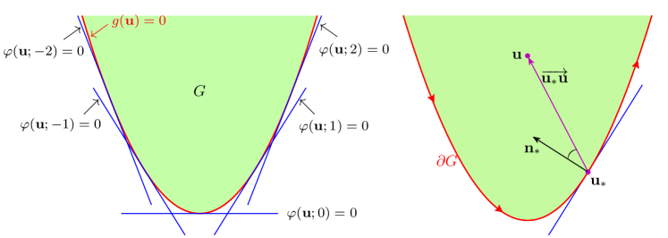
Figure 1: Illustrations for Example 3.4.

Example 3.4.

Consider the simple example mentioned in Eq. 8–Eq. 9, i.e., $G=\{{\bf u}=(u_{1},u_{2})^{\top}\in\mathbb{R}^{2}:~{}g({\bf u})=u_{2}-u_{1}^{2}>0\}$. According to Theorem 3.2, the GQL representation of $G$ is

(30) $$G_{*}=\left\{{\bf u}=(u_{1},u_{2})^{\top}\in\mathbb{R}^{2}:~{}\varphi({\bf u};\theta_{*})=u_{2}-2u_{1}\theta_{*}+\theta_{*}^{2}>0~{}~{}\forall\theta_{*}\in\mathbb{R}\right\}.$$

As such, we gain the linearity by introducing the extra free auxiliary variable $\theta_{*}$. To understand the intrinsic mechanisms, we draw the graph of the region $G$ and its boundary curve $\partial G=\{{\bf u}:g({\bf u})=0\}$ on the $u_{1}$–$u_{2}$ plane in Fig. 1. We also plot the graphs of $\{{\bf u}:\varphi({\bf u};\theta_{*})=0\}$ for several special values of $\theta_{*}\in\{\pm 2,\pm 1,0\}$ in the left subfigure of Fig. 1. It is observed that all the lines $\{{\bf u}:\varphi({\bf u};\theta_{*})=0\}$ are tangent to the parabolic curve $\partial G$, which exactly forms an envelope of the tangent lines.

Let ${\bf u}_{*}=(\theta_{*},\theta_{*}^{2})^{\top}$ denote an arbitrary point on $\partial G$. One can verify that ${\bf n}_{*}=(-2\theta_{*},1)^{\top}$ is an inward-pointing normal vector of $\partial G$ at ${\bf u}_{*}$, and

$$\varphi({\bf u};\theta_{*})={\bf u}\cdot{\bf n}_{*}-{\bf u}_{*}\cdot{\bf n_{*}}=\overrightarrow{{\bf u}_{*}{\bf u}}\cdot{\bf n}_{*}>0\quad\forall{\bf u}\in G.$$

Imagine we are walking along the boundary $\partial G$ in the direction shown in the right subfigure of Fig. 1, then the region $G$ always lie entirely on the left side of the tangent lines, namely, the angle between the two vectors $\overrightarrow{{\bf u}_{*}{\bf u}}$ and ${\bf n}_{*}$ is always less than $90^{\circ}$ for all ${\bf u}\in G$ and all ${\bf u}_{*}\in\partial G$. This intuitively interprets the GQL representation Eq. 30 from the geometric viewpoint.

3.2 Concepts from geometry and convex sets

Let us recall some concepts and results from theory of geometry and convex analysis [28, 42, 19].

A hyperplane in $\mathbb{R}^{N}$ is a plane of dimension $N-1$. Let ${\bf n}_{*}\neq{\bf 0}$ denote a normal vector of a hyperplane $H$, and let ${\bf u}_{*}$ be a point on $H$. Then $H$ can be expressed as $H=\{{\bf u}\in\mathbb{R}^{N}:({\bf u}-{\bf u}_{*})\cdot{\bf n}_{*}=0\}$, and it divides $\mathbb{R}^{N}$ into two halfspaces: $H^{+}=\{{\bf u}\in\mathbb{R}^{N}:({\bf u}-{\bf u}_{*})\cdot{\bf n}_{*}\geq 0\}$ and $H^{-}=\{{\bf u}\in\mathbb{R}^{N}:({\bf u}-{\bf u}_{*})\cdot{\bf n}_{*}\leq 0\}$.

Definition 3.5 (Supporting Hyperplane and Halfspace).

The hyperplane $H=\{{\bf u}\in\mathbb{R}^{N}:({\bf u}-{\bf u}_{*})\cdot{\bf n}_{*}=0\}$ through ${\bf u}_{*}\in\partial G$ is called a supporting hyperplane to $G$ at ${\bf u}_{*}$, if $G$ lies in one of the two closed halfspaces determined by $H$. Furthermore, if the normal vector ${\bf n}_{*}$ points towards $G$, then the closed halfspace containing $G$ is $H^{+}=\{{\bf u}\in\mathbb{R}^{N}:({\bf u}-{\bf u}_{*})\cdot{\bf n}_{*}\geq 0\}$ and is called a closed supporting halfspace to $G$. See Fig. 2.

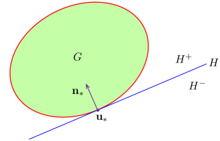
Figure 2: Supporting hyperplane and halfspace.

Theorem 3.6 (Supporting Hyperplane Theorem [28]).

If $G$ is a convex set and ${\rm int}(G)\neq\emptyset$, then for any ${\bf u}_{*}\in\partial G$, there exists a supporting hyperplane to $G$ at ${\bf u}_{*}$.

Remark 3.7.

If the boundary $\partial G$ is smooth at a point ${\bf u}_{*}$, then the supporting hyperplane to $G$ at ${\bf u}_{*}$ is unique and coincide with the tangent [42, 19].

3.3 GQL framework

We are now in the position to establish the GQL framework.

3.3.1 A special case

Inspired by Example 3.4, we first consider a special case that $G$ is either open or closed with differentiable boundary. The general case will be discussed in Section 3.3.2.

Theorem 3.8.

Suppose that 1 holds, the region $G$ is either open or closed, and $\partial G$ is differentiable. Then $G$ has the following GQL representation:

(31) $$G_{*}=\Big{\{}{\bf u}\in\mathbb{R}^{N}:~{}({\bf u}-{\bf u}_{*})\cdot{\bf n}_{*}\succ 0~{}~{}\forall{\bf u}_{*}\in\partial G\Big{\}},$$

where the symbol “$\succ$” is taken as “$>$” if $G$ is open, or as “$\geq$” if $G$ is closed, and ${\bf n}_{*}$ is only dependent on ${\bf u}_{*}$ and denotes an inward-pointing normal vector of $\partial G$ at ${\bf u}_{*}$.

The proof of Theorem 3.8 is presented in Appendix A. Following the proof, one can further extend the above result to any closed convex region $G$, whose boundary is typically not everywhere smooth so that the supporting hyperplanes at each nonsmooth boundary point are not unique. Let ${\mathcal{N}}({\bf u}_{*})$ denote the set of the inward-pointing unit normal vectors of all the supporting hyperplanes to $G$ at ${\bf u}_{*}\in\partial G$. Then one can prove that

(32) $$G=\left\{{\bf u}\in\mathbb{R}^{N}:~{}\left({\bf u}-{\bf u}_{*}\right)\cdot{\bf n}\geq 0~{}~{}\forall{\bf n}\in{\mathcal{N}}({\bf u}_{*}),~{}~{}\forall{\bf u}_{*}\in\partial G\right\}.$$

This means any closed convex region is the intersection of all its closed supporting halfspaces [28]. However, the representation Eq. 32 is not applicable to a general convex region that is neither closed nor open (e.g. the invariant regions in Eq. 13 and Eq. 19). Moreover, the representation Eq. 32 requires the information of all the supporting hyperplanes at each nonsmooth boundary point, which can be difficult to explicitly formulate or verify, so that Eq. 32 is not desirable for bound-preserving study. A practical GQL representation for more general regions will be derived in Section 3.3.2.

3.3.2 General case

Consider a general convex region $G$ that may be not necessarily open or closed and its boundary may be not everywhere smooth. Note that the boundary of a convex region can be partitioned into several pieces, each of which can be locally represented as the graph of a convex function (with respect to a suitable supporting hyperplane). Recall that any convex function is locally Lipschitz continuous and twice differentiable almost everywhere, according to the classical theorems of Rademacher and Alexandrov (cf. [37]). Based on these facts and for convenience, we make a considerably mild assumption on the convex invariant region $G$. We assume that the boundary of $G$ is piecewise $C^{1}$, and without loss of generality, for each $i\in\{1,\dots,I\}$, the function $g_{i}({\bf u})$ in Eq. 27 is $C^{1}$ at any points on

$${\mathcal{S}}_{i}:=\partial G\cap\partial G_{i},\qquad\mbox{with}\quad G_{i}:=\left\{{\bf u}\in\mathbb{R}^{N}:~{}g_{i}({\bf u})\succ 0\right\},$$

where $\{{\mathcal{S}}_{i}\}$ are $C^{1}$ hypersurfaces in $\mathbb{R}^{N}$ and constitute the smooth pieces of $\partial G$, i.e., $\partial G=\cup_{1\leq i\leq I}{\mathcal{S}}_{i}$. Notice that in general, ${\mathcal{S}}_{i}$ may not equal $\partial G_{i}$, the region $G_{i}$ may be not convex, and $G$ may be neither open nor closed; see an example in Fig. 3. These make our following discussions nontrivial.

We remark that $G_{i}=\{{\bf u}:g_{i}({\bf u})\geq 0\}$ is closed for $i\in\widehat{\mathbb{I}}$, and $G_{i}=\{{\bf u}:g_{i}({\bf u})>0\}$ is open for $i\in{\mathbb{I}}$. Since for each $i\in{\mathbb{I}}$, the set $G_{i}$ is not necessarily convex, there is a possibility that $G$ may not be entirely contained in an open supporting halfspace at ${\bf u}_{*}\in{\mathcal{S}}_{i}$. This issue is avoid if the open region $\cap_{i\in\mathbb{I}}G_{i}$ is convex, which is satisfied by all the examples in Section 2 and implies that

(33) $$G\cap\left(\cup_{{\bf u}_{*}\in{\mathcal{S}}_{i}}\{{\bf u}\in\mathbb{R}^{N}:~{}({\bf u}-{\bf u}_{*})\cdot{\bf n}_{i*}=0\}\right)=\emptyset\quad\forall i\in{\mathbb{I}},$$

where ${\bf n}_{i*}$ is an inward-pointing normal vector of ${\mathcal{S}}_{i}$ at ${\bf u}_{*}$.

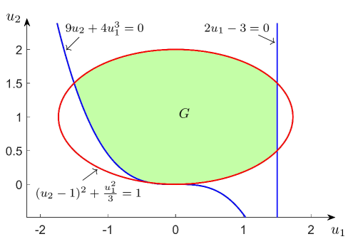
Figure 3: A convex region $G$ involving nonlinear constraints. $G=\{{\bf u}\in\mathbb{R}^{2}:g_{1}({\bf u})\geq 0,~{}g_{2}({\bf u})\geq 0,~{}g_{3}({\bf u})>0\}$ with $g_{1}({\bf u})=3-2u_{1}$, $g_{2}({\bf u})=9u_{2}+4u_{1}^{3}$, and $g_{3}({\bf u})=1-{u_{1}^{2}}/3-(u_{2}-1)^{2}$.

Theorem 3.9.

Suppose that 1 holds, condition Eq. 33 is satisfied when $\mathbb{I}\neq\emptyset$, and the boundary of $G$ is piecewise $C^{1}$. Then the region $G$ has the following GQL representation:

(34) $$G_{*}=\Big{\{}{\bf u}\in\mathbb{R}^{N}:~{}\big{(}{\bf u}-{\bf u}_{*}\big{)}\cdot{\bf n}_{i*}\succ 0~{}~{}\forall{\bf u}_{*}\in{\mathcal{S}}_{i},~{}1\leq i\leq I\Big{\}},$$

where the symbol “$\succ$” is taken as “$>$” if $i\in\mathbb{I}$, or as “$\geq$” if $i\in\widehat{\mathbb{I}}$; the nonzero vector ${\bf n}_{i*}$ denotes an inward-pointing normal vector of ${\mathcal{S}}_{i}$ at ${\bf u}_{*}$.

Proof 3.10.

The proof is divided into three steps.

(i) Prove that $G\subseteq G_{*}$. Let $\partial G=:\widetilde{\partial G}\cup\widehat{\partial G}$ with $\widetilde{\partial G}$ denoting the set of smooth boundary points and $\widehat{\partial G}$ the set of nonsmooth boundary points. For any ${\bf u}_{*}\in\widetilde{\partial G}\cap{\mathcal{S}}_{i}$, the hyperplane $({\bf u}-{\bf u}_{*})\cdot{\bf n}_{i*}=0$ supports the region $G$, implying that

(35) $$G\subseteq\left\{{\bf u}\in\mathbb{R}^{N}:~{}({\bf u}-{\bf u}_{*})\cdot{\bf n}_{i*}\geq 0\right\}\quad\forall{\bf u}_{*}\in\widetilde{\partial G}\cap{\mathcal{S}}_{i},~{}1\leq i\leq I.$$

Next, we consider an arbitrary nonsmooth boundary point ${\bf u}_{*}\in\widehat{\partial G}\cap{\mathcal{S}}_{i}$. There exists a sequence of smooth boundary points $\{{\bf u}_{*}^{(j)}\}_{j\in\mathbb{N}}\subset\widetilde{\partial G}\cap{\mathcal{S}}_{i}$ such that $\mathop{\lim}\limits_{j\to\infty}{\bf u}_{*}^{(j)}={\bf u}_{*}.$ For every ${\bf u}_{*}^{(j)}$, it follows from Eq. 35 that

(36) $$\big{(}{\bf u}-{\bf u}_{*}^{(j)}\big{)}\cdot{\bf n}_{i,{\bf u}_{*}^{(j)}}\geq 0\qquad\forall{\bf u}\in G,$$

where ${\bf n}_{i,{\bf u}_{*}^{(j)}}$ is the inward-pointing normal vector of ${\mathcal{S}}_{i}$ at ${\bf u}_{*}^{(j)}$ satisfying $\mathop{\lim}\limits_{j\to\infty}{\bf n}_{i,{\bf u}_{*}^{(j)}}={\bf n}_{i*}.$ Taking the limit $j\to+\infty$ in Eq. 36 gives

$$({\bf u}-{\bf u}_{*})\cdot{\bf n}_{i*}\geq 0\quad\forall{\bf u}\in G\quad\forall{\bf u}_{*}\in\widehat{\partial G}\cap{\mathcal{S}}_{i},~{}1\leq i\leq I,$$

which along with Eq. 35 yields

(37) $$G\subseteq\left\{{\bf u}\in\mathbb{R}^{N}:~{}\big{(}{\bf u}-{\bf u}_{*}\big{)}\cdot{\bf n}_{i*}\geq 0~{}~{}\forall{\bf u}_{*}\in{\mathcal{S}}_{i},~{}1\leq i\leq I\right\}.$$

Based on Eq. 33, we then conclude that $G\subseteq G_{*}$.

(ii) Prove that $G_{*}\subseteq{\rm cl}(G)$ by contradiction. Assume that $G_{*}\not\subseteq{\rm cl}(G)$, namely, there exists ${\bf u}_{0}\in G_{*}$ but ${\bf u}_{0}\notin{\rm cl}(G)$. According to the theory of convex optimization [5], the minimum of the convex function $\zeta({\bf u}):=\frac{1}{2}\|{\bf u}-{\bf u}_{0}\|^{2}$ over the closed convex region ${\rm cl}(G)$ is attained at certain boundary point ${\bf u}_{*0}\in\partial G$. In other words, ${\bf u}_{*0}$ is a solution to the following optimization problem

(38) $$\mathop{\rm minimize}\limits_{{\bf u}\in{\rm cl}(G)}{}{} \zeta({\bf u})$$

$${\rm subject~{}to}{}{} -g_{i}({\bf u})<0~{}~{}\forall i\in\mathbb{I};\quad-g_{i}({\bf u})\leq 0~{}~{}\forall i\in\widehat{\mathbb{I}}.$$

Since the function $-g_{i}({\bf u})$ is not necessarily convex, the problem Eq. 38 is generally not the standard form of convex optimization. Note that the condition ${\rm int}(G)\neq\emptyset$ ensures the Slater condition [5, 4] is satisfied. The Karush–Kuhn–Tucker (KKT) conditions [5, 4] tell us that there exist $\{\lambda_{0},\lambda_{1},\dots,\lambda_{I}\}$ such that

(39) $$0=\nabla\zeta({\bf u}_{*0})-\sum_{i=1}^{I}\lambda_{i}\nabla g_{i}({\bf u}_{*0}),$$

(40) $$0=\lambda_{i}g_{i}({\bf u}_{*0}),\qquad 1\leq i\leq I,$$

(41) $$\lambda_{i}\geq 0,\qquad 0\leq i\leq I.$$

Define $\mathbb{I}_{+}:=\{1\leq i\leq I:\lambda_{i}>0\}$. Obviously $\mathbb{I}_{+}\neq\emptyset$; otherwise $\lambda_{i}=0$ for all $1\leq i\leq I$, so that ${\bf u}_{*0}-{\bf u}_{0}=\nabla\zeta({\bf u}_{*0})={\bf 0}$ which leads to the contradiction $\partial G\ni{\bf u}_{*0}={\bf u}_{0}\notin{\rm cl}(G)$. This also implies ${\bf u}_{*0}\neq{\bf u}_{0}$. Let ${\bf n}_{i*0}$ be the inward-pointing normal vector of ${\mathcal{S}}_{i}$ at ${\bf u}_{*0}$. Since there exist $\mu_{i}\geq 0$ such that $\nabla g_{i}({\bf u}_{*,0})=\mu_{i}{\bf n}_{i*0}$, condition Eq. 39 can be rewritten as

(42) $${\bf u}_{*0}-{\bf u}_{0}=\sum_{i\in\mathbb{I}_{+}}\lambda_{i}\mu_{i}{\bf n}_{i*0}.$$

Thanks to Eq. 40, we obtain $g_{i}({\bf u}_{*0})=0$ for all $i\in\mathbb{I}_{+}$, which along with ${\bf u}_{*0}\in\partial G$ leads to

$${\bf u}_{*0}\in{\mathcal{S}}_{i}=\partial G_{i}\cap\partial G\qquad\forall i\in\mathbb{I}_{+}.$$

Because ${\bf u}_{0}\in G_{*}$, we then have $({\bf u}_{0}-{\bf u}_{*0})\cdot{\bf n}_{i*0}\succ 0$ for all $i\in\mathbb{I}_{+}$. This, together with Eq. 42 and ${\bf u}_{*0}\neq{\bf u}_{0}$, leads to a contradiction:

$$0 >-\left\|{\bf u}_{0}-{\bf u}_{*0}\right\|_{2}^{2}=\left({\bf u}_{0}-{\bf u}_{*0}\right)\cdot\left({\bf u}_{*0}-{\bf u}_{0}\right)$$

$$=\left({\bf u}_{0}-{\bf u}_{*0}\right)\cdot\left(\sum_{i\in\mathbb{I}_{+}}\lambda_{i}\mu_{i}{\bf n}_{i*0}\right)=\sum_{i\in\mathbb{I}_{+}}\lambda_{i}\mu_{i}\left({\bf u}_{0}-{\bf u}_{*0}\right)\cdot{\bf n}_{i*0}\geq 0.$$

Thus the assumption $G_{*}\not\subseteq{\rm cl}(G)$ is incorrect. We have $G_{*}\subseteq{\rm cl}(G)$.

(iii) Prove that $G_{*}\subseteq G$. If $\mathbb{I}=\emptyset$, then $G$ is a closed region and $G={\rm cl}(G)$. We immediately obtain $G_{*}\subseteq G$ from step (ii) of this proof. In the following, we focus on $\mathbb{I}\neq\emptyset$ and prove $G_{*}\subseteq G$ by contradiction. Assume that there exists ${\bf u}_{0}\in G_{*}$ but ${\bf u}_{0}\notin G$. Because we have already shown $G_{*}\subseteq{\rm cl}(G)$ in step (ii) of this proof, we then get ${\bf u}_{0}\in{\rm cl}(G)\setminus G=\partial G$. Note that ${\bf u}_{0}\in G_{*}$ implies

$$\left({\bf u}_{0}-{\bf u}_{*}\right)\cdot{\bf n}_{i*}>0\qquad\forall{\bf u}_{*}\in{\mathcal{S}}_{i},~{}~{}~{}\forall i\in\mathbb{I},$$

which leads to ${\bf u}_{0}\notin{\mathcal{S}}_{i}=\partial G_{i}\cap\partial G$ for all $i\in\mathbb{I}$. It follows that ${\bf u}_{0}\notin\partial G_{i}$ for all $i\in\mathbb{I}$. Note for $i\in\mathbb{I}$, one has ${\bf u}_{0}\in{\rm cl}(G)\subseteq{\rm cl}(G_{i})$, which gives

(43) $${\bf u}_{0}\in{\rm cl}(G_{i})\setminus\partial G_{i}=G_{i}\quad\forall i\in\mathbb{I}.$$

On the other hand, ${\bf u}_{0}\in{\rm cl}(G)\subseteq\cap_{i\in\mathbb{\widehat{I}}}G_{i}$, which along with Eq. 43 implies ${\bf u}_{0}\in(\cap_{i\in\mathbb{I}}G_{i})\cap(\cap_{i\in\mathbb{\widehat{I}}}G_{i})=G$. This contradicts the assumption that ${\bf u}_{0}\notin G$. Hence the assumption is incorrect, and we have $G_{*}\subseteq G$.

Combining the conclusions proven in steps (i) and (iii) gives $G=G_{*}$.

Remark 3.11.

If we replace ${\mathcal{S}}_{i}$ with ${\mathcal{S}}_{i}\cap\widetilde{\partial G}$ for $i\in\widehat{\mathbb{I}}$ in Eq. 34, Theorem 3.9 remains valid, because for $i\in\widehat{\mathbb{I}}$ we have $\{{\bf u}:({\bf u}-{\bf u}_{*})\cdot{\bf n}_{i*}\geq 0~{}\forall{\bf u}_{*}\in{\mathcal{S}}_{i}\}=\{{\bf u}:({\bf u}-{\bf u}_{*})\cdot{\bf n}_{i*}\geq 0~{}\forall{\bf u}_{*}\in{\mathcal{S}}_{i}\cap\widetilde{\partial G}\}.$

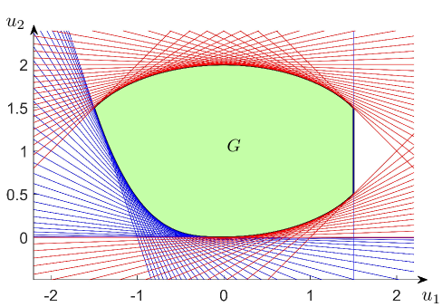
Figure 4: Illustration of the GQL representation for the convex region $G$ given in Fig. 3. The blue (resp. red) lines correspond to closed (resp. open) supporting halfspaces.

Remark 3.12.

An illustration of the GQL representation Eq. 34 is shown in Fig. 4. Different from Eq. 32, the GQL representation Eq. 34 involves only at most $N$ rather than all the supporting halfspaces at each nonsmooth “junction” point. This makes the GQL representation Eq. 34 easier to formulate or construct. Besides, Theorem 3.9 does not require $G$ to be closed or open.

Remark 3.13 (Significance of GQL).

Compared to the original form Eq. 27 of the invariant region $G$ with nonlinear constraints, its equivalent GQL representation $G_{*}$ in Eq. 34 is described with only linear constraints. Such linearity gives the GQL representation some significant advantages over the original form Eq. 27 in analyzing and designing bound-preserving schemes; see Sections 5 and 6.

4 Construction of geometric quasilinearization

With three methods and several examples, this section discusses how to construct GQL for convex invariant regions.

4.1 Methods for constructing GQL representations

Based on Theorems 3.9 and 3.2, we introduce three simple effective methods for constructing the GQL representation of $G$.

4.1.1 Gradient-based method

The first method is based on the following result, which is a direct consequence of Theorem 3.9.

Theorem 4.1.

Assume that the hypotheses of Theorem 3.9 hold and

(44) $$\nabla g_{i}({\bf u}_{*})\neq{\bf 0}~{}~{}\forall{\bf u}_{*}\in{\mathcal{S}}_{i},~{}1\leq i\leq I,$$

then the invariant region $G$ is exactly equivalent to

(45) $$G_{*}=\Big{\{}{\bf u}\in\mathbb{R}^{N}:~{}\varphi_{i}({\bf u};{\bf u}_{*})\succ 0~{}~{}\forall{\bf u}_{*}\in{\mathcal{S}}_{i},~{}1\leq i\leq I\Big{\}},$$

where the function $\varphi_{i}$ is linear with respect to $\bf u$, defined by

(46) $$\varphi_{i}({\bf u};{\bf u}_{*}):=\left({\bf u}-{\bf u}_{*}\right)\cdot\nabla g_{i}({\bf u}_{*}).$$

Theorem 4.1 says if $\{\nabla g_{i}\}$ are computable and satisfy Eq. 44, then we can directly obtain the GQL representation in the form Eq. 45 with Eq. 46.

In some cases, it is, however, difficult to calculate the gradients of nonlinear functions $\{g_{i}\}$, e.g., the implicit functions in Eq. 19 and Eq. 26. This motivates us to propose the following cross-product method based on suitable parametrization of the hypersurface ${\mathcal{S}}_{i}$. The use of parametrization can also help to reduce or decouple the free auxiliary variables, which is highly desirable for bound-preserving applications; see the examples in Section 4.2 and Remark 4.6.

4.1.2 Cross-product method

Assume that for each $i$ the hypersurface ${\mathcal{S}}_{i}$ has the following parametric expression

(47) $${\mathcal{S}}_{i}=\left\{{\bf u}_{*}={\bf U}_{i}({\bm{\theta}}_{i*}):~{}{\bm{\theta}}_{i*}\in\Theta_{i}\subseteq\mathbb{R}^{N-1}\right\},$$

where ${\bf U}_{i}$ is a $C^{1}$ vector function defined on the parameter domain $\Theta_{i}$ with ${\mathcal{S}}_{i}$ being the function range. Denote $\theta_{i*}^{(k)}$ as the $k$th component of ${\bm{\theta}}_{i*}$. For each $i$, we define

$${\bm{\tau}}_{i,k}({\bm{\theta}}_{i*}):=\frac{\partial{\bf U}_{i}}{\partial\theta_{i*}^{(k)}},\qquad 1\leq k\leq N-1.$$

The vectors $\{{\bm{\tau}}_{i,k}({\bm{\theta}}_{i*}):1\leq k\leq N-1\}$ are ($N-1$) tangent vectors of the hypersurface ${\mathcal{S}}_{i}$ and generate its local tangent space at ${\bf u}_{*}$. Then, the normal vector of ${\mathcal{S}}_{i}$ at ${\bf u}_{*}$ can be constructed using the $(N-1)$-ary analogue of the cross product (cf. [46, Pages 83–85]) in $\mathbb{R}^{N}$:

$${\bf n}_{i*}=\delta_{i*}\bigwedge\limits_{k=1}^{N-1}{\bm{\tau}}_{i,k}({\bm{\theta}}_{i*}):=\delta_{i*}{\bm{\tau}}_{i,1}({\bm{\theta}}_{i*})\times{\bm{\tau}}_{i,2}({\bm{\theta}}_{i*})\times\cdots\times{\bm{\tau}}_{i,N-1}({\bm{\theta}}_{i*}),$$

where $\delta_{i*}$ is a nonzero factor which may be used to simplify the final formula or/and to adjust the sign such that ${\bf n}_{i*}$ is directed towards the interior of $G$.

As a direct consequence of Theorem 3.9, the following result holds.

Theorem 4.2.

Suppose the hypotheses of Theorem 3.9 hold and

$$\bigwedge\limits_{k=1}^{N-1}{\bm{\tau}}_{i,k}({\bm{\theta}}_{i*})\neq{\bf 0}~{}~{}\forall{\bm{\theta}}_{i*}\in\Theta_{i},~{}1\leq i\leq I,$$

then the region $G$ is exactly equivalent to

(48) $$G_{*}=\Big{\{}{\bf u}\in\mathbb{R}^{N}:~{}\varphi_{i}({\bf u};{\bm{\theta}}_{i*})\succ 0~{}~{}\forall{\bm{\theta}}_{i*}\in\Theta_{i},~{}1\leq i\leq I\Big{\}},$$

where the function $\varphi_{i}$ is linear with respect to $\bf u$, defined by

(49) $$\varphi_{i}({\bf u};{\bm{\theta}}_{i*}):=\Big{(}{\bf u}-{\bf U}_{i}({\bm{\theta}}_{i*})\Big{)}\cdot\left(\delta_{i*}\bigwedge\limits_{k=1}^{N-1}{\bm{\tau}}_{i,k}({\bm{\theta}}_{i*})\right).$$

Remark 4.3.

In many cases, there exists a natural (usually physics-based) parametrization of the hypersurface ${\mathcal{S}}_{i}$, typically with the primitive quantities as parametric variables; see the examples in Section 4.2. The advantages of using the parametric form Eq. 47 in the GQL representation will become more clear in those examples and the bound-preserving applications in Sections 5 and 6.

4.1.3 Constructive method

For completeness, we also summarize the constructive approach and its variant as our third method. Recall that Theorem 3.2 has told us: if we can construct linear functions $\varphi_{i}({\bf u};{\bm{\theta}}_{i*})$, $1\leq i\leq I$, such that Eq. 29 holds, then the GQL representation of $G$ is Eq. 28. The constructive approach does not require the assumptions in Theorems 4.1 and 4.2, but often needs some empirical trial-and-error techniques to find the qualified $\{\varphi_{i}\}$. In practice, one can use the proposed three methods in a hybrid way: first formally formulate $\{\varphi_{i}\}$ via either Eq. 46 or Eq. 49 and then verify Eq. 29. Such a hybrid approach is efficient, as it may exempt the assumptions in Theorems 4.1 and 4.2 and also avoid the trial-and-error procedure.

4.2 Examples of GQL representations

We give several examples for constructing GQL representations of convex invariant regions.

Example 1: Euler and Navier–Stokes systems

Theorem 4.4.

For the 1D Euler and Navier–Stokes systems, the GQL representation of the invariant region $G$ in Eq. 12 is given by

(50) $$G_{*}=\left\{{\bf u}=(\rho,m,E)^{\top}:~{}\rho>0,~{}~{}\varphi({\bf u};v_{*})>0~{}~{}\forall v_{*}\in\mathbb{R}\right\}$$

with $\varphi({\bf u};v_{*}):=E-mv_{*}+\rho\frac{v_{*}^{2}}{2}$ being linearly dependent on $\bf u$.

Proof 4.5.

We respectively use the three methods proposed in Section 4.1 to derive the GQL representation for this example. Note the first constraint in Eq. 12 is linear.

(i) Gradient-based method. For the second constraint in Eq. 12, the gradient $\nabla g({\bf u})=(\frac{m^{2}}{2\rho^{2}},-\frac{m}{\rho},1)^{\top}$, and the associated boundary hypersurface ${\mathcal{S}}=\{{\bf u}_{*}=(\rho_{*},m_{*},E_{*})^{\top}:\rho_{*}>0,~{}g({\bf u}_{*})=0\}$ can be parameterized as

(51) $${\mathcal{S}}=\left\{{\bf u}_{*}=\left(\rho_{*},\rho_{*}v_{*},\frac{\rho_{*}}{2}v_{*}^{2}\right)^{\top}:\rho_{*}>0,~{}v_{*}\in\mathbb{R}\right\}.$$

For ${\bf u}_{*}\in{\mathcal{S}}$ and ${\bf u}=(\rho,m,E)^{\top}$, we have

(52) $$({\bf u}-{\bf u}_{*})\cdot\nabla g({\bf u}_{*})=(\rho-\rho_{*})\frac{v_{*}^{2}}{2}+(m-\rho_{*}v_{*})(-v_{*})+E-\frac{\rho_{*}}{2}v_{*}^{2}=\varphi({\bf u};v_{*}).$$

By Theorem 4.1, we obtain the GQL representation Eq. 50 of $G$.

(ii) Cross-product method. Based on the parametrization of $\mathcal{S}$ in Eq. 51, we can compute the normal vector of ${\mathcal{S}}$ at ${\bf u}_{*}$ by cross product

$$\frac{\partial{\bf u}_{*}}{\partial\rho_{*}}\times\frac{\partial{\bf u}_{*}}{\partial v_{*}}=\left(1,v_{*},\frac{1}{2}v_{*}^{2}\right)^{\top}\times\left(0,\rho_{*},\rho_{*}v_{*}\right)^{\top}=\rho_{*}\left(\frac{1}{2}v_{*}^{2},-v_{*},1\right)^{\top}=:\frac{1}{\delta_{*}}{\bf n}_{*},$$

where $\delta_{*}=1/\rho_{*}$ is a nonzero factor. By Theorem 4.2 and $({\bf u}-{\bf u}_{*})\cdot{\bf n}_{*}=\varphi({\bf u};v_{*})$, we get the GQL representation Eq. 50.

(iii) Constructive method. Observe that

(53) $$\varphi({\bf u};v_{*})=E-mv_{*}+\rho\frac{v_{*}^{2}}{2}=\frac{\rho}{2}\left(v_{*}-\frac{m}{\rho}\right)^{2}+g({\bf u})\geq g({\bf u}),$$

which implies $\min_{v_{*}\in\mathbb{R}}\varphi({\bf u};v_{*})=g({\bf u})$ for $\rho>0$. According to Theorem 3.2, we also achieve the GQL representation Eq. 50.

Remark 4.6.

Note only one free auxiliary variable $v_{*}$ explicitly appears in the GQL representation Eq. 50. This is benefited from the use of parametric form Eq. 51.

Remark 4.7 (Physical Interpretation of GQL).

It seems that the linear function $\varphi({\bf u};v_{*})$ plays an energy-like role from a physical point of view. For the present example, $\varphi({\bf u};v_{*})=\frac{1}{2}\rho(v-v_{*})^{2}+\rho e$, which represents the total energy in the reference frame moving at a velocity of $v_{*}$.

We now utilize the cross-product method to construct the GQL representation of the invariant region $\widetilde{G}$ in Eq. 13, where the minimum entropy principle $S({\bf u}):=p\rho^{-\Gamma}\geq S_{min}$ is also included.

Theorem 4.8.

For the 1D Euler and Navier–Stokes systems, the GQL representation of the invariant region $\widetilde{G}$ in Eq. 13 is given by

(54) $$\widetilde{G}_{*}=\Big{\{}{\bf u}=(\rho,m,E)^{\top}:~{}\rho>0,~{}~{}\widetilde{\varphi}({\bf u};\rho_{*},v_{*})\geq 0~{}~{}\forall\rho_{*}\in\mathbb{R}^{+}~{}~{}\forall v_{*}\in\mathbb{R}\Big{\}}$$

with $\widetilde{\varphi}({\bf u};\rho_{*},v_{*}):={\bf u}\cdot{\bf n}_{*}+S_{min}\rho_{*}^{\Gamma}$ and ${\bf n}_{*}:=\big{(}\frac{v_{*}^{2}}{2}-\frac{S_{min}\Gamma\rho_{*}^{\Gamma-1}}{\Gamma-1},~{}-v_{*},~{}1\big{)}^{\top}$.

Proof 4.9.

We only need to handle the nonlinear constraint $\widetilde{g}({\bf u})>0$ in Eq. 13, with the boundary hypersurface $\widetilde{\mathcal{S}}:=\{{\bf u}_{*}=(\rho_{*},m_{*},E_{*}):\rho_{*}>0,~{}\widetilde{g}({\bf u}_{*})=0\}$. Motivated from the equivalence of $\widetilde{g}({\bf u})=0$ and $p=S_{min}\rho^{\Gamma}$, we find a natural physics-based parametrization of $\widetilde{\mathcal{S}}$ as

$$\widetilde{\mathcal{S}}=\left\{{\bf u}_{*}=\left(\rho_{*},~{}\rho_{*}v_{*},~{}\frac{1}{2}\rho_{*}v_{*}^{2}+\frac{S_{min}\rho_{*}^{\Gamma}}{\Gamma-1}\right)^{\top}:~{}\rho_{*}>0,~{}v_{*}\in\mathbb{R}\right\}.$$

Then we can derive the normal vector ${\bf n}_{*}$ of ${\mathcal{S}}$ at ${\bf u}_{*}$ by cross product:

$$\frac{\partial{\bf u}_{*}}{\partial\rho_{*}}\times\frac{\partial{\bf u}_{*}}{\partial v_{*}}=\left(1,~{}v_{*},~{}\frac{S_{min}\Gamma\rho_{*}^{\Gamma-1}}{\Gamma-1}+\frac{v_{*}^{2}}{2}\right)^{\top}\times\left(0,~{}\rho_{*},~{}\rho_{*}v_{*}\right)^{\top}=\rho_{*}{\bf n}_{*}.$$

By Theorem 4.2 and $({\bf u}-{\bf u}_{*})\cdot{\bf n}_{*}=\widetilde{\varphi}({\bf u};\rho_{*},v_{*})$, we obtain the GQL representation Eq. 54.

Example 2: M1 model of radiative transfer

Theorem 4.10.

For the gray M1 moment system of radiative transfer, the GQL representation of the invariant region $G$ in Eq. 15 is given by

(55) $$G_{*}=\left\{{\bf u}=(E_{r},{\mathbfcal F}_{r})^{\top}\in\mathbb{R}^{4}:~{}E_{r}-{\mathbfcal F}_{r}\cdot{\bm{\theta}}_{*}\geq 0~{}~{}\forall{\bm{\theta}}_{*}\in\mathbb{S}_{1}({\bf 0})\right\}$$

with $\mathbb{S}_{1}({\bf 0}):=\{{\bm{x}}\in\mathbb{R}^{3}:\|{\bm{x}}\|=1\}$ denoting the unit 3D sphere.

Proof 4.11.

The constructive method is used for this example. The Cauchy–Schwarz inequality yields

$$\varphi({\bf u};{\bm{\theta}}_{*}):=E_{r}-{\mathbfcal F}_{r}\cdot{\bm{\theta}}_{*}\geq g({\bf u})\qquad\forall{\bm{\theta}}_{*}\in\mathbb{S}_{1}({\bf 0}),$$

where equality holds for ${\mathbfcal F}_{r}\neq{\bm{0}}$ with ${\bm{\theta}}_{*}={\mathbfcal F}_{r}/\|{\mathbfcal F}_{r}\|$ and for ${\mathbfcal F}_{r}={\bm{0}}$ with any ${\bm{\theta}}_{*}$. Thus, $\min_{{\bm{\theta}}_{*}\in\mathbb{S}_{1}(0)}\varphi({\bf u};{\bm{\theta}}_{*})=g({\bf u})$, and by Theorem 3.2 we get the GQL representation Eq. 55.

Example 3: Relativistic hydrodynamic system

Theorem 4.12.

For the 1D RHD system Eq. 16, the GQL representation of the invariant region $G$ in Eq. 18 is given by

(56) $$G_{*}=\left\{{\bf u}=(D,m,E)^{\top}:D>0,~{}\varphi({\bf u};v_{*})>0~{}~{}\forall v_{*}\in(-1,1)\right\}$$

with $\varphi({\bf u};v_{*}):=E-mv_{*}-D\sqrt{1-v_{*}^{2}}$ being a linear function of $\bf u$.

Proof 4.13.

The first constraint in Eq. 18 is linear. We deal with the second one by the constructive method. The Cauchy–Schwarz inequality implies

$$\varphi({\bf u};v_{*})\geq E-\sqrt{D^{2}+m^{2}}\sqrt{v_{*}^{2}+\left(\sqrt{1-v_{*}^{2}}\right)^{2}}=E-\sqrt{D^{2}+m^{2}}=g({\bf u}),$$

where equality holds if $v_{*}=m/\sqrt{D^{2}+m^{2}}$. This means $\min_{v_{*}\in(-1,1)}\varphi({\bf u};v_{*})=g({\bf u})$. According to Theorem 3.2, we get the GQL representation Eq. 56.

We now utilize the cross-product method to construct the GQL representation of the invariant region $\widetilde{G}$ in Eq. 19, where the minimum entropy principle is also included as a constraint.

Theorem 4.14.

For the 1D RHD system Eq. 16, the GQL representation of the invariant region $\widetilde{G}$ in Eq. 19 is given by

(57) $$\widetilde{G}_{*}=\Big{\{}{\bf u}=(D,m,E)^{\top}:~{}\rho>0,~{}~{}\widetilde{\varphi}({\bf u};\rho_{*},v_{*})\geq 0~{}~{}\forall\rho_{*}\in\mathbb{R}^{+}~{}~{}\forall v_{*}\in(-1,1)\Big{\}}$$

with $\widetilde{\varphi}({\bf u};\rho_{*},v_{*}):={\bf u}\cdot{\bf n}_{*}+S_{min}\rho_{*}^{\Gamma}$ and ${\bf n}_{*}:=\left(-\sqrt{1-v_{*}^{2}}\big{(}1+\frac{S_{min}\Gamma\rho_{*}^{\Gamma-1}}{\Gamma-1}\big{)},-v_{*},1\right)^{\top}$.

Proof 4.15.

We only need to tackle the second and third constraints in Eq. 19. For the third constraint $\widetilde{g}({\bf u})\geq 0$, the corresponding boundary hypersurface is $\widetilde{\mathcal{S}}:=\{{\bf u}_{*}=(\rho_{*},m_{*},E_{*}):\rho_{*}>0,~{}g({\bf u}_{*})>0,~{}\widetilde{g}({\bf u}_{*})=0\}$. Based on the equivalence of $\widetilde{g}({\bf u})=0$ and $p=S_{min}\rho^{\Gamma}$, we obtain a natural physics-based parametrization of $\widetilde{\mathcal{S}}$, namely,

$$\widetilde{\mathcal{S}}=\left\{{\bf u}_{*}=\left(\frac{\rho_{*}}{\sqrt{1-v_{*}^{2}}},~{}\frac{\Big{(}\rho_{*}+\frac{S_{min}\Gamma\rho_{*}^{\Gamma}}{\Gamma-1}\Big{)}v_{*}}{1-v_{*}^{2}},~{}\frac{\rho_{*}+\frac{S_{min}\Gamma\rho_{*}^{\Gamma}}{\Gamma-1}}{1-v_{*}^{2}}-S_{min}\rho_{*}^{\Gamma}\right)^{\top}:~{}\rho_{*}>0,~{}v_{*}\in(-1,1)\right\}.$$

We can then derive the normal vector ${\bf n}_{*}$ of ${\mathcal{S}}$ at ${\bf u}_{*}$ by cross product:

$$\frac{\partial{\bf u}_{*}}{\partial\rho_{*}}\times\frac{\partial{\bf u}_{*}}{\partial v_{*}} =\frac{1}{\delta_{*}}{\bf n}_{*},\quad\mbox{with}~{}~{}\delta_{*}:=(1-v_{*})^{5/2}\left(\rho_{*}+\frac{S_{min}\Gamma}{\Gamma-1}\rho_{*}^{\Gamma}(1+v_{*}^{2}-\Gamma v_{*}^{2})\right)^{-1}.$$

By Theorem 4.2 and $({\bf u}-{\bf u}_{*})\cdot{\bf n}_{*}=\widetilde{\varphi}({\bf u};\rho_{*},v_{*})$, the GQL representation for $\widetilde{g}({\bf u})\geq 0$ is

(58) $$\widetilde{\varphi}({\bf u};\rho_{*},v_{*})\geq 0\qquad\forall\rho_{*}\in\mathbb{R}^{+},\quad\forall v_{*}\in\mathbb{R}.$$

Note that $S_{min}>0$ and

$$g({\bf u})>g({\bf u})-\frac{S_{min}}{\Gamma-1}\left(\frac{D^{2}}{\sqrt{D^{2}+m^{2}}}\right)^{\Gamma}=\widetilde{\varphi}\left({\bf u};\frac{D^{2}}{\sqrt{D^{2}+m^{2}}},\frac{m}{\sqrt{D^{2}+m^{2}}}\right),$$

which means that Eq. 58 also implies $g({\bf u})>0$ in Eq. 19. That is, the second and third constraints in Eq. 19 can be equivalently represented by Eq. 58. Therefore, we obtain the GQL representation Eq. 57.

Example 4: Ten-moment Gaussian closure system

Theorem 4.16.

For the 2D ten-moment Gaussian closure system Eq. 20, the GQL representation of the invariant region $G$ in Eq. 22 is given by

(59) $$G_{*}=\Big{\{}{\bf u}\in\mathbb{R}^{6}:\rho>0,~{}\varphi({\bf u};{\bm{z}},{\bm{v}}_{*})>0~{}~{}\forall{\bm{v}}_{*}\in\mathbb{R}^{2}~{}~{}\forall{\bm{z}}\in\mathbb{R}^{2}\setminus\{{\bf 0}\}\Big{\}},$$

where ${\bf u}:=(\rho,{\bm{m}},E_{11},E_{12},E_{22})^{\top}$, and the function $\varphi({\bf u};{\bm{z}},{\bm{v}}_{*})$ is linear with respect to $\bf u$:

(60) $$\varphi({\bf u};{\bm{z}},{\bm{v}}_{*}):={\bm{z}}^{\top}\left({\bf E}-{\bm{m}}\otimes{\bm{v}}_{*}+\rho\frac{{\bm{v}}_{*}\otimes{\bm{v}}_{*}}{2}\right){\bm{z}}.$$

Proof 4.17.

We only need to deal with the nonlinear constraint in Eq. 22. Note that

$$\varphi({\bf u};{\bm{z}},{\bm{v}}_{*})={\bm{z}}^{\top}\left({\bf E}-\frac{{\bm{m}}\otimes{\bm{m}}}{2\rho}\right){\bm{z}}+\frac{\rho}{2}\left|{\bm{z}}\cdot\left({\bm{v}}_{*}-\frac{\bm{m}}{\rho}\right)\right|^{2},$$

which implies $\min_{{\bm{v}}_{*}\in\mathbb{R}^{2}}\varphi({\bf u};{\bm{z}},{\bm{v}}_{*})={\bm{z}}^{\top}\big{(}{\bf E}-\frac{{\bm{m}}\otimes{\bm{m}}}{2\rho}\big{)}{\bm{z}}$. By Theorem 3.2, we immediately obtain the GQL representation Eq. 59.

Example 5: Ideal MHD system

Theorem 4.18.

For the ideal MHD system Eq. 23, the GQL representation of the invariant region $G$ in Eq. 24 is given by

(61) $$G_{*}=\Big{\{}{\bf u}=(\rho,{\bm{m}},{\bf B},E)^{\top}\in\mathbb{R}^{8}:~{}\rho>0,~{}\varphi({\bf u};{\bm{v}}_{*},{\bf B}_{*})>0~{}~{}\forall{\bm{v}}_{*},{\bf B}_{*}\in\mathbb{R}^{3}\Big{\}}$$

with $\varphi({\bf u};{\bm{v}}_{*},{\bf B}_{*}):={\bf u}\cdot{\bf n}_{*}+\frac{\|{\bf B}_{*}\|^{2}}{2}$ and ${\bf n}_{*}:=\big{(}\frac{\|{\bm{v}}_{*}\|^{2}}{2},-{\bm{v}}_{*},-{\bf B}_{*},1\big{)}^{\top}.$

Proof 4.19.

We use to the gradient-based method. For the nonlinear constraint in Eq. 24, the gradient of $g({\bf u})$ is $\nabla g({\bf u})=\big{(}\frac{\|{\bm{m}}\|^{2}}{2\rho^{2}},-\frac{\bm{m}}{\rho},-{\bf B},1\big{)}^{\top},$ and the corresponding boundary hypersurface is ${\mathcal{S}}:=\{{\bf u}_{*}=(\rho_{*},{\bm{m}}_{*},{\bf B}_{*},E_{*})^{\top}:\rho_{*}>0,g({\bf u}_{*})=0\}$. Based on the equivalence of $g({\bf u})=0$ and $p=0$, we obtain a natural physics-based parametrization of ${\mathcal{S}}$, namely,

$${\mathcal{S}}=\left\{{\bf u}_{*}=\left(\rho_{*},\rho_{*}{\bm{v}}_{*},{\bf B}_{*},\frac{1}{2}\big{(}\rho_{*}\|{\bm{v}}_{*}\|^{2}+\|{\bf B}_{*}\|^{2}\big{)}\right)^{\top}:\rho_{*}>0,~{}{\bm{v}}_{*}\in\mathbb{R}^{3},~{}{\bf B}_{*}\in\mathbb{R}^{3}\right\}.$$

For ${\bf u}_{*}\in{\mathcal{S}}$ and ${\bf u}=(\rho,{\bm{m}},{\bf B},E)^{\top}$, we have $({\bf u}-{\bf u}_{*})\cdot\nabla g({\bf u}_{*})=\varphi({\bf u};{\bm{v}}_{*},{\bf B}_{*}).$ By Theorem 4.1, we obtain the GQL representation Eq. 61.

Example 6: Relativistic MHD system

Theorem 4.20.

For the relativistic MHD system Eq. 25, the GQL representation of the invariant region $G$ in Eq. 26 is given by

(62) $$G_{*}=\Big{\{}{\bf u}\in\mathbb{R}^{8}:~{}D>0,~{}\varphi({\bf u};{\bm{v}}_{*},{\bf B}_{*})>0~{}~{}\forall{\bf B}_{*}\in\mathbb{R}^{3}~{}~{}\forall{\bm{v}}_{*}\in\mathbb{B}_{1}({\bf 0})\Big{\}},$$

where ${\bf u}=(D,{\bm{m}},{\bf B},E)^{\top}$, $\mathbb{B}_{1}({\bf 0}):=\{{\bm{x}}\in\mathbb{R}^{3}:\|{\bm{x}}\|\leq 1\}$ is a unit 3D ball, and the linear function $\varphi({\bf u};{\bm{v}}_{*},{\bf B}_{*}):={\bf u}\cdot{\bf n}_{*}+p_{m}^{*}$ with

(63) $$p_{m}^{*}:=\frac{1}{2}\left({(1-{\|{\bm{v}}_{*}\|}^{2})\|{\bf B}_{*}\|^{2}+({\bm{v}}_{*}\cdot{\bf B}_{*})^{2}}\right),$$

(64) $${\bf n}_{*}:=\left(-\sqrt{1-{\|{\bm{v}}_{*}\|}^{2}},~{}-{\bm{v}}_{*},~{}-(1-{\|{\bm{v}}_{*}\|}^{2}){\bf B}_{*}-({\bm{v}}_{*}\cdot{\bf B}_{*}){\bm{v}}_{*},~{}1\right)^{\top}.$$

Note that $p_{m}^{*}$ and ${\bf n}_{*}$ only depend on the free auxiliary variables $({\bm{v}}_{*},{\bf B}_{*})$.

Proof 4.21.

As shown in [57], the region $G$ in Eq. 26 can be equivalently represented as

(65) $$G=\left\{{\bf u}\in\mathbb{R}^{8}:~{}D>0,~{}g_{2}({\bf u})>0,~{}p({\bf u})>0\right\}$$

with $g_{2}({\bf u}):=E-\sqrt{D^{2}+\|{\bm{m}}\|^{2}}$. Although the implicit function $p({\bf u})$ defined in Eq. 7 can not be explicitly formulated, the corresponding boundary hypersurface ${\mathcal{S}}:=\{{\bf u}_{*}=(D_{*},{\bm{m}}_{*},{\bf B}_{*},E_{*})^{\top}:D_{*}>0,g_{2}({\bf u}_{*})>0,p({\bf u}_{*})=0\}$ has an explicit physics-based parameterization:

$${\mathcal{S}}=\Big{\{}{\bf u}_{*} =\Big{(}\rho_{*}\gamma_{*},~{}\rho_{*}\gamma_{*}^{2}{\bm{v}}_{*}+\|{\bf B}_{*}\|^{2}{\bm{v}}_{*}-({\bm{v}}_{*}\cdot{\bf B}_{*}){\bf B}_{*},~{}{\bf B}_{*},$$

$$\qquad\rho_{*}\gamma_{*}^{2}+\|{\bf B}_{*}\|^{2}-p_{m}^{*}\Big{)}^{\top}:\rho_{*}>0,~{}{\bf B}_{*}\in\mathbb{R}^{3},~{}{\bm{v}}_{*}\in\mathbb{B}_{1}({\bf 0})\Big{\}}$$

with $p_{m}^{*}$ defined in Eq. 63 and $\gamma_{*}:=(1-\|{\bm{v}_{*}}\|^{2})^{\frac{1}{2}}$. This parameterization is helpful for dealing with the highly nonlinear constraint $p({\bf u})>0$ by the cross-product method. For $1\leq i\leq 3$, denote ${\bf e}_{i}:=(\delta_{1i},\delta_{2i},\delta_{3i})$ with $\delta_{ij}$ being the Kronecker delta. Taking the partial derivatives of ${\bf u}_{*}$ with respect to the parametric variables $\{\rho_{*},{\bm{v}}_{*},{\bf B}_{*}\}$ gives

$$\frac{\partial{\bf u}_{*}}{\partial\rho_{*}} =\left(\gamma_{*},~{}\gamma_{*}^{2}{\bm{v}}_{*},~{}0,~{}0,0,~{}\gamma_{*}^{2}\right)^{\top},$$

$$\frac{\partial{\bf u}_{*}}{\partial v_{i*}} =\Big{(}\rho_{*}\gamma_{*}^{3}v_{i*},(\rho_{*}\gamma_{*}^{2}+\|{\bf B}_{*}\|^{2}){\bf e}_{i}+2\rho_{*}\gamma_{*}^{4}v_{i*}{\bm{v}}_{*}-B_{i*}{\bf B}_{*},0,0,0,2\rho_{*}\gamma_{*}^{4}v_{i*}-B_{i*}({\bm{v}}_{*}\cdot{\bf B}_{*})+\|{\bf B}_{*}\|^{2}v_{i*}\Big{)}^{\top},$$

$$\frac{\partial{\bf u}_{*}}{\partial B_{i*}} =\Big{(}0,~{}-({\bm{v}}_{*}\cdot{\bf B}_{*}){\bf e}_{i}+2B_{i*}{\bm{v}}_{*}-v_{i}{\bf B}_{*},~{}{\bf e}_{i},B_{i*}(1+\|{\bm{v}}_{*}\|^{2})-v_{i*}({\bm{v}}_{*}\cdot{\bf B}_{*})\Big{)},~{}~{}1\leq i\leq 3,$$

which are all perpendicular to the nonzero vector ${\bf n}_{*}$ defined in Eq. 64. This means ${\bf n}_{*}$ is parallel to the cross product $\frac{\partial{\bf u}_{*}}{\partial\rho_{*}}\times\big{(}\bigwedge\limits_{i=1}^{3}\frac{\partial{\bf u}_{*}}{\partial v_{i*}}\big{)}\times\big{(}\bigwedge\limits_{i=1}^{3}\frac{\partial{\bf u}_{*}}{\partial B_{i*}}\big{)}$, implying that ${\bf n}_{*}$ is a normal vector of ${\mathcal{S}}$ at ${\bf u}_{*}$. It can be verified that ${\bf n}_{*}$ is always directed towards the concave side of $\mathcal{S}$. By Theorem 4.2 and $({\bf u}-{\bf u}_{*})\cdot{\bf n}_{*}=\varphi({\bf u};{\bm{v}}_{*},{\bf B}_{*})$, we know that the GQL representation for $p({\bf u})>0$ is

(66) $$\varphi({\bf u};{\bm{v}}_{*},{\bf B}_{*})>0\quad\forall{\bf B}_{*}\in\mathbb{R}^{3}\quad\forall{\bm{v}}_{*}\in\mathbb{B}_{1}({\bf 0}).$$

If taking ${\bm{v}}_{*}={\bm{m}}/\sqrt{D^{2}+\|{\bm{m}}\|^{2}}$ and ${\bf B}_{*}={\bf 0}$, we obtain $\varphi({\bf u};{\bm{v}}_{*},{\bf B}_{*})=g_{2}({\bf u})$, which means that Eq. 66 also implies $g_{2}({\bf u})>0$ in Eq. 65. In other words, the second and third constraints in Eq. 65 can be equivalently represented by Eq. 66. Therefore, we obtain the GQL representation Eq. 62.

5 Geometric quasilinearization for bound-preserving analysis

This section applies the GQL approach to analyze the bound-preserving property of numerical schemes and shows its remarkable advantages over direct and traditional approaches by diverse examples covering different schemes of three PDE systems in one and two dimensions. We only focus on first-order schemes for illustrative purposes, while the GQL approach is readily extensible to high-order schemes. The application of GQL to design high-order bound-preserving scheme will also be explored in Section 6 for the multicomponent MHD system, to further demonstrate its capability in addressing challenging bound-preserving problems that could not be coped with by direct approaches.

5.1 Example 1: Euler system

Consider a finite volume scheme

(67) $$\bar{\bf u}_{j}^{n+1}=\bar{\bf u}_{j}^{n}-\sigma\left(\hat{\bf f}_{j+\frac{1}{2}}-\hat{\bf f}_{j-\frac{1}{2}}\right),$$

for solving the 1D Euler system Eq. 11 on a uniform spatial mesh $\{[x_{j-1/2},x_{j+1/2}]\}$ with $\sigma:={\Delta t}/{\Delta x}$ denoting the ratio of the temporal step-size $\Delta t$ to the spatial step-size $\Delta x$. Here $\bar{\bf u}_{j}^{n}$ is an approximation to the average of ${\bf u}(x,t_{n})$ on cell $[x_{j-1/2},x_{j+1/2}]$, and $\hat{\bf f}_{j+1/2}$ is a numerical flux at $x_{j+1/2}$. For system Eq. 11, it holds that ${\bf f}({\bf u})=v{\bf u}+p(0,1,v)^{\top}$, which will be used in the following analysis.

We apply the GQL approach to analyze the bound-preserving property of the scheme Eq. 67 with the invariant region $G$ defined in Eq. 12. Thanks to the GQL representation in Theorem 4.4, we have

(68) $$G=G_{*}=\left\{{\bf u}:~{}{\bf u}\cdot{\bf e}_{1}>0,~{}{\bf u}\cdot{\bf n}_{*}>0~{}~{}\forall v_{*}\in\mathbb{R}\right\}$$

with ${\bf e}_{1}:=(1,0,0)^{\top}$ and ${\bf n}_{*}:=\big{(}\frac{v_{*}^{2}}{2},-v_{*},1\big{)}^{\top}$. GQL transfers the bound-preserving problem into preserving the positivity of ${\bf u}\cdot{\bf e}_{1}$ and ${\bf u}\cdot{\bf n}_{*}$, which are all linear with respect to $\bf u$ and helpful for bound-preserving study.

Example 1.1: Lax–Friedrichs scheme

To clearly illustrate the basic idea, we begin with the simple Lax–Friedrichs scheme with the numerical flux $\hat{\bf f}_{j+1/2}$ taken as

(69) $$\hat{\bf f}^{\mathrm{LF}}(\bar{\bf u}_{j}^{n},\bar{\bf u}_{j+1}^{n}):=\frac{1}{2}\Big{(}{\bf f}(\bar{\bf u}_{j}^{n})+{\bf f}(\bar{\bf u}_{j+1}^{n})-\alpha_{n}(\bar{\bf u}_{j+1}^{n}-\bar{\bf u}_{j}^{n})\Big{)},$$

where $\alpha_{n}:=\max_{j}\alpha(\bar{\bf u}_{j}^{n})$ with $\alpha({\bf u}):=|v|+\sqrt{\Gamma p/\rho}$ being the spectral radius of the Jacobian matrix $\partial{\bf f}/\partial{\bf u}$. Given that $\bar{\bf u}_{j}^{n}\in G$ for all $j$, we wish $\bar{\bf u}_{j}^{n+1}\in G$.

For respectively ${\bf n}={\bf e}_{1}$ and ${\bf n}={\bf n}_{*}$, thanks to the linearity of ${\bf u}\cdot{\bf n}$ we obtain

$$\bar{\bf u}_{j}^{n+1}\cdot{\bf n}=\left(1-\sigma\alpha_{n}\right)\bar{\bf u}_{j}^{n}\cdot{\bf n}+\frac{\sigma}{2}\Big{(}\alpha_{n}\bar{\bf u}_{j+1}^{n}\cdot{\bf n}-{\bf f}(\bar{\bf u}_{j+1}^{n})\cdot{\bf n}+\alpha_{n}\bar{\bf u}_{j-1}^{n}\cdot{\bf n}+{\bf f}(\bar{\bf u}_{j-1}^{n})\cdot{\bf n}\Big{)}.$$

The problem boils down to control the effect of ${\bf f}(\bar{\bf u}_{\pm}^{n})\cdot{\bf n}$ by using the positivity of $\bar{\bf u}_{j\pm 1}^{n}\cdot{\bf n}$. For any ${\bf u}\in G$, we have ${\bf u}\cdot{\bf n}>0$ and

$$\pm{\bf f}({\bf u})\cdot{\bf e}_{1} =\pm v({\bf u}\cdot{\bf e}_{1})<\alpha({\bf u}){\bf u}\cdot{\bf e}_{1},$$

$$\pm{\bf f}({\bf u})\cdot{\bf n}_{*} =\pm v({\bf u}\cdot{\bf n}_{*})\pm p(v-v_{*})$$

$$\leq|v|({\bf u}\cdot{\bf n}_{*})+\left(\frac{1}{2}\rho(v-v_{*})^{2}+\rho e\right)\frac{p}{\rho\sqrt{2e}}$$

$$=\left(|v|+\frac{p}{\rho\sqrt{2e}}\right){\bf u}\cdot{\bf n}_{*}<\alpha({\bf u}){\bf u}\cdot{\bf n}_{*},$$

which yield $\alpha_{n}\bar{\bf u}_{j\pm 1}^{n}\cdot{\bf n}\mp{\bf f}(\bar{\bf u}_{j\pm 1}^{n})\cdot{\bf n}>0$. Thus we obtain $\bar{\bf u}_{j}^{n+1}\cdot{\bf n}>(1-\sigma\alpha_{n})\bar{\bf u}_{j}^{n}\cdot{\bf n}\geq 0$ provided that $\sigma\alpha_{n}\leq 1$. This proves that the scheme Eq. 67 with the Lax–Friedrichs flux Eq. 69 is bound-preserving under the standard CFL condition $\sigma\alpha_{n}\leq 1$.

Remark 5.1.

As we have seen, unlike the traditional approaches that require substituting the target scheme into the original nonlinear constraint of $G$ in Eq. 12, the GQL approach skillfully transfers all the constraints into linear ones which can be investigated in a unified way.

Example 1.2: Gas-kinetic scheme

In order to demonstrate the advantages of the GQL approach in bound-preserving analysis, we consider a challenging example—the gas-kinetic scheme with the numerical flux $\hat{\bf f}_{j+1/2}$ taken as

(70) $$\hat{\bf f}^{\mathrm{GK}}(\bar{\bf u}_{j}^{n},\bar{\bf u}_{j+1}^{n}):={\bf f}^{+}(\bar{\bf u}_{j}^{n})+{\bf f}^{-}(\bar{\bf u}_{j+1}^{n}).$$

(71) $${\bf f}^{\pm}({\bf u}):=\int_{\mathbb{R}^{\pm}}\int_{\mathbb{R}^{M}}\begin{pmatrix}w\\ w^{2}\\ \frac{w}{2}(w^{2}+{\bm{\xi}}^{2})\end{pmatrix}F(w,{\bm{\xi}};{\bf u}){\rm d}{\bm{\xi}}{\rm d}w,$$

where $w$ is the particle velocity, ${\bm{\xi}}\in\mathbb{R}^{M}$ denotes the internal variables whose degrees of freedom $M=(3-\Gamma)/(\Gamma-1)$, the equilibrium distribution function $F$ is

(72) $$F(w,{\bm{\xi}};{\bf u}):=\rho\left(\frac{\lambda}{\pi}\right)^{\frac{M+1}{2}}{\rm e}^{-\lambda\left((w-v)^{2}+\|{\bm{\xi}}\|^{2}\right)}$$

with $\rho$ being the fluid velocity, $v$ being the fluid velocity, and $\lambda=\rho/(2p)$.

In a traditional approach [49], the bound-preserving property of this scheme was studied by: (i) first, evaluating the integration Eq. 71 as

(73) $${\bf f}^{\pm}({\bf u})=\rho\begin{pmatrix}\frac{v}{2}{\rm erfc}(\mp\sqrt{\lambda}v)\pm\frac{1}{2}\frac{{\rm e}^{-\lambda v^{2}}}{\sqrt{\pi\lambda}}\\ \left(\frac{v^{2}}{2}+\frac{1}{4\lambda}\right){\rm erfc}(\mp\sqrt{\lambda}v)\pm\frac{v}{2}\frac{{\rm e}^{-\lambda v^{2}}}{\sqrt{\pi\lambda}}\\ \left(\frac{v^{3}}{4}+\frac{M+3}{8\lambda}v\right){\rm erfc}(\mp\sqrt{\lambda}v)\pm\left(\frac{v^{2}}{4}+\frac{M+2}{8\lambda}\right)\frac{{\rm e}^{-\lambda v^{2}}}{\sqrt{\pi\lambda}}\end{pmatrix}$$

with ${\rm erfc}(x):=\frac{2}{\sqrt{\pi}}\int_{x}^{+\infty}{\rm e}^{-w^{2}}dw$; (ii) then, plugging the numerical flux Eq. 70 with Eq. 73 into Eq. 67 and splitting the scheme Eq. 67 into two steps; (iii) and finally checking the bound-preserving properties of the split schemes by verifying the original constraints of $G$ in Eq. 12. For this scheme, verifying the nonlinear constraint in Eq. 12 are difficult and complicated.

Benefited from its linear feature, the GQL approach is highly effective for this challenging case. For ${\bf n}={\bf e}_{1}$ or ${\bf n}={\bf n}_{*}$, thanks to the linearity of ${\bf u}\cdot{\bf n}$ we obtain

$$\bar{\bf u}_{j}^{n+1}\cdot{\bf n}=\bar{\bf u}_{j}^{n}\cdot{\bf n}-\sigma\left({\bf f}^{+}(\bar{\bf u}_{j}^{n})-{\bf f}^{-}(\bar{\bf u}_{j}^{n})\right)\cdot{\bf n}-\sigma{\bf f}^{-}(\bar{\bf u}_{j+1}^{n})\cdot{\bf n}+\sigma{\bf f}^{+}(\bar{\bf u}_{j-1}^{n})\cdot{\bf n}.$$

Note that for any ${\bf u}\in G$, we have $F(w,{\bm{\xi}};{\bf u})>0$ and

$$\pm{\bf f}^{\pm}({\bf u})\cdot{\bf e}_{1} =\int_{\mathbb{R}^{\pm}}\int_{\mathbb{R}^{M}}|w|F(w,{\bm{\xi}};{\bf u}){\rm d}{\bm{\xi}}{\rm d}w>0,$$

$$\pm{\bf f}^{\pm}({\bf u})\cdot{\bf n}_{*} =\int_{\mathbb{R}^{\pm}}\int_{\mathbb{R}^{M}}\frac{|w|}{2}\Big{(}(w-v_{*})^{2}+\|{\bm{\xi}}\|^{2}\Big{)}F(w,{\bm{\xi}};{\bf u}){\rm d}{\bm{\xi}}{\rm d}w>0.$$

It follows, for ${\bf n}={\bf e}_{1}$ and ${\bf n}={\bf n}_{*}$ respectively, that

(74) $$\bar{\bf u}_{j}^{n+1}\cdot{\bf n}>\bar{\bf u}_{j}^{n}\cdot{\bf n}-\sigma\left({\bf f}^{+}(\bar{\bf u}_{j}^{n})-{\bf f}^{-}(\bar{\bf u}_{j}^{n})\right)\cdot{\bf n}.$$

Next, we use the positivity of ${\bf u}\cdot{\bf n}$ to bound the effect of $\left({\bf f}^{+}({\bf u})-{\bf f}^{-}({\bf u})\right)\cdot{\bf n}$ as follows:

$$\left({\bf f}^{+}({\bf u})-{\bf f}^{-}({\bf u})\right)\cdot{\bf e}_{1} =({\bf u}\cdot{\bf e}_{1})\left(\frac{\lambda}{\pi}\right)^{\frac{1}{2}}\left(\int_{\mathbb{R}}|w|{\rm e}^{-\lambda(w-v)^{2}}{\rm d}w\right)$$

$$\leq({\bf u}\cdot{\bf e}_{1})\left(\frac{\lambda}{\pi}\right)^{\frac{1}{2}}\left(\int_{\mathbb{R}}(|v|+|w-v|){\rm e}^{-\lambda(w-v)^{2}}{\rm d}w\right)$$

$$=({\bf u}\cdot{\bf e}_{1})\left(|v|+1/\sqrt{\pi\lambda}\right)<a({\bf u}){\bf u}\cdot{\bf e}_{1},$$

$$\left({\bf f}^{+}({\bf u})-{\bf f}^{-}({\bf u})\right)\cdot{\bf n}_{*} =\int_{\mathbb{R}}\int_{\mathbb{R}^{M}}\frac{|w|}{2}\Big{(}(w-v_{*})^{2}+\|{\bm{\xi}}\|^{2}\Big{)}F(w,{\bm{\xi}};{\bf u}){\rm d}{\bm{\xi}}{\rm d}w$$

$$\leq\int_{\mathbb{R}}\int_{\mathbb{R}^{M}}\frac{|v|+|w-v|}{2}\Big{(}(w-v_{*})^{2}+\|{\bm{\xi}}\|^{2}\Big{)}F(w,{\bm{\xi}};{\bf u}){\rm d}{\bm{\xi}}{\rm d}w$$

$$=|v|({\bf u}\cdot{\bf n}_{*})+\frac{\rho}{2\sqrt{\pi\lambda}}\left((v-v_{*})^{2}+\frac{M+2}{2\lambda}\right)$$

$$\leq|v|({\bf u}\cdot{\bf n}_{*})+\frac{\rho}{2\sqrt{\pi\lambda}}\left((v-v_{*})^{2}+\frac{M+1}{2\lambda}\right)\frac{M+2}{M+1}$$

$$=\left(|v|+\frac{M+2}{M+1}(\pi\lambda)^{-\frac{1}{2}}\right)({\bf u}\cdot{\bf n}_{*})<a({\bf u})({\bf u}\cdot{\bf n}_{*}).$$

This implies $\left({\bf f}^{+}(\bar{\bf u}_{j}^{n})-{\bf f}^{-}(\bar{\bf u}_{j}^{n})\right)\cdot{\bf n}<\alpha(\bar{\bf u}_{j}^{n})\bar{\bf u}_{j}^{n}\cdot{\bf n}\leq\alpha_{n}\bar{\bf u}_{j}^{n}\cdot{\bf n}$. It then follows from Eq. 74 that $\bar{\bf u}_{j}^{n+1}\cdot{\bf n}>(1-\sigma\alpha_{n})\bar{\bf u}_{j}^{n}\cdot{\bf n}\geq 0$ provided that $\sigma\alpha_{n}\leq 1$. This proves that the scheme Eq. 67 with the gas-kinetic flux Eq. 70 is bound-preserving under the standard CFL condition $\sigma\alpha_{n}\leq 1$.

Remark 5.2.

The linearity of GQL brought by introducing the free auxiliary variable $v_{*}$ gives remarkable advantages in our above analysis. Because $v_{*}$ is independent of all the system variables $\bf u$, it can freely move cross the integrals. We no longer need to substitute a complicated scheme into the nonlinear function $g({\bf u})$ in Eq. 12 to verify $g({\bf u})>0$. Instead, we work on the simpler but equivalent linear constraint ${\bf u}\cdot{\bf n}_{*}>0$. The interested readers may compare the above analysis based on GQL and the traditional analysis in [49].

5.2 Example 2: Navier–Stokes system

Consider the scheme

(75) $$\bar{\bf u}_{j}^{n+1}=\bar{\bf u}_{j}^{n}-\sigma\big{(}\hat{\bf f}_{j+\frac{1}{2}}-\hat{\bf f}_{j-\frac{1}{2}}\big{)}+\frac{\Delta t}{\Delta x^{2}}\frac{\eta}{\tt Re}{\bf H}_{j}$$

with ${\bf H}_{j}:={\bf r}(\bar{\bf u}_{j+1}^{n})-2{\bf r}(\bar{\bf u}_{j}^{n})+{\bf r}(\bar{\bf u}_{j-1}^{n})$, for solving the 1D dimensionless compressible Navier–Stokes equations Eq. 14. Here $\hat{\bf f}_{j+1/2}$ is taken as a bound-preserving numerical flux for the 1D Euler system Eq. 11, for example, the Lax–Friedrichs flux Eq. 69 or the gas-kinetic flux Eq. 70, which satisfy: if $\bar{\bf u}_{j}^{n}\in G$ for all $j$, then

$$\big{(}\hat{\bf f}_{j+\frac{1}{2}}-\hat{\bf f}_{j-\frac{1}{2}}\big{)}\cdot{\bf n}<\alpha_{n}\bar{\bf u}_{j}^{n}\cdot{\bf n}\qquad\forall j$$

holds for respectively ${\bf n}={\bf e}_{1}$ and ${\bf n}={\bf n}_{*}$, according to the analysis in Section 5.1. Thus we have

(76) $$\bar{\bf u}_{j}^{n+1}\cdot{\bf n}>(1-\sigma\alpha_{n})\bar{\bf u}_{j}^{n}\cdot{\bf n}+\frac{\Delta t}{\Delta x^{2}}\frac{\eta}{\tt Re}{\bf H}_{j}\cdot{\bf n}.$$

Thanks to GQL, we clearly see that the bound-preserving essence is to control the potentially negative term ${\bf H}_{j}\cdot{\bf n}$ by the positive term $\bar{\bf u}_{j}^{n}\cdot{\bf n}$. Note ${\bf H}_{j}\cdot{\bf e}_{1}=0$, thereby $\bar{\bf u}_{j}^{n+1}\cdot{\bf e}_{1}>(1-\sigma\alpha_{n})\bar{\bf u}_{j}^{n}\cdot{\bf e}_{1}\geq 0$ if $\sigma\alpha_{n}\leq 1$. For any ${\bf u}\in G$ and $v_{*}\in\mathbb{R}$, we have

$$-\frac{v_{*}^{2}}{2}<{\bf r}({\bf u})\cdot{\bf n}_{*}=\frac{1}{2}(v-v_{*})^{2}+\frac{\Gamma}{{\tt Pr}~{}\eta}e-\frac{v_{*}^{2}}{2}\leq\max\left\{1,\frac{\Gamma}{{\tt Pr}~{}\eta}\right\}\frac{1}{\rho}({\bf u}\cdot{\bf n}_{*})-\frac{v_{*}^{2}}{2}.$$

This gives

$${\bf H}_{j}\cdot{\bf n}_{*} =\Big{(}{\bf r}(\bar{\bf u}_{j+1}^{n})\cdot{\bf n}_{*}+{\bf r}(\bar{\bf u}_{j-1}^{n})\cdot{\bf n}_{*}\Big{)}-2{\bf r}(\bar{\bf u}_{j}^{n})\cdot{\bf n}_{*}$$

$$\geq\left(-\frac{v_{*}^{2}}{2}-\frac{v_{*}^{2}}{2}\right)-2\left(\max\left\{1,\frac{\Gamma}{{\tt Pr}~{}\eta}\right\}\frac{1}{\bar{\rho}_{j}^{n}}(\bar{\bf u}_{j}^{n}\cdot{\bf n}_{*})-\frac{v_{*}^{2}}{2}\right)$$

$$=-\frac{2}{\bar{\rho}_{j}^{n}}\max\left\{1,\frac{\Gamma}{{\tt Pr}~{}\eta}\right\}(\bar{\bf u}_{j}^{n}\cdot{\bf n}_{*}).$$

It then follows from Eq. 76 that

$$\bar{\bf u}_{j}^{n+1}\cdot{\bf n}_{*}>(1-\sigma\alpha_{n})\bar{\bf u}_{j}^{n}\cdot{\bf n}_{*}-\frac{\Delta t}{\Delta x^{2}}\frac{\eta}{\tt Re}\frac{2}{\bar{\rho}_{j}^{n}}\max\left\{1,\frac{\Gamma}{{\tt Pr}~{}\eta}\right\}(\bar{\bf u}_{j}^{n}\cdot{\bf n}_{*}).$$

We then immediately have $\bar{\bf u}_{j}^{n+1}\cdot{\bf n}_{*}>0$, provided that

(77) $$\alpha_{n}\frac{\Delta t}{\Delta x}+\frac{\Delta t}{\Delta x^{2}}\frac{2}{\bar{\rho}_{j}^{n}{\tt Re}}\max\left\{\eta,\frac{\Gamma}{{\tt Pr}}\right\}\leq 1.$$

In conclusion, the scheme Eq. 75 is bound-preserving under condition Eq. 77.

Remark 5.3.

A standard approach for handling bound-preserving problems with multiple terms (e.g., convection term and diffusion term [66], or convection term and source term [69]) is based on decomposing the schemes into a convex combination of some subterms, and then enforcing all the subterms in $G$. This may lead to stricter conditions on the time step-size $\Delta t$. Since the linear feature of GQL has already naturally incorporated the convexity of $G$ into the GQL representation, technical convex decomposition is not necessary in the GQL approach.

5.3 Example 3: Ten-moment Gaussian closure system

Consider the scheme

(78) $$\bar{\bf u}_{ij}^{n+1}=\bar{\bf u}_{ij}^{n}-\sigma_{1}\big{(}\hat{\bf f}_{1,i+\frac{1}{2},j}-\hat{\bf f}_{1,i-\frac{1}{2},j}\big{)}-\sigma_{2}\big{(}\hat{\bf f}_{2,i,j+\frac{1}{2}}-\hat{\bf f}_{2,i,j-\frac{1}{2}}\big{)},$$

for solving the 2D Gaussian closure equations Eq. 20 on a uniform Cartesian mesh $\{[x_{i-1/2},x_{i+1/2}]\times[y_{j-1/2},y_{j+1/2}]\}$, with $\sigma_{1}=\frac{\Delta t}{\Delta x}$, $\sigma_{2}=\frac{\Delta t}{\Delta y}$. Here $\bar{\bf u}_{ij}^{n}$ denotes an approximation to the average of ${\bf u}(x,y,t_{n})$ on each cell, and the Lax-Friedrichs numerical fluxes are considered, i.e.

(79) $$\hat{\bf f}_{1,i+1/2,j}=\hat{\bf f}^{\rm LF}_{1}(\bar{\bf u}_{ij}^{n},\bar{\bf u}_{i+1,j}^{n}),\quad\hat{\bf f}_{2,i,j+1/2}=\hat{\bf f}^{\rm LF}_{2}(\bar{\bf u}_{ij}^{n},\bar{\bf u}_{i,j+1}^{n}),$$

(80) $$\hat{\bf f}^{\rm LF}_{\ell}({\bf u}^{L},{\bf u}^{R}):=\frac{1}{2}\Big{(}{\bf f}_{\ell}({\bf u}^{L})+{\bf f}_{\ell}({\bf u}^{R})-\alpha_{\ell,n}({\bf u}^{R}-{\bf u}^{L})\Big{)},\quad\ell=1,2,$$

where $\alpha_{\ell,n}=\max_{ij}\alpha_{\ell}(\bar{\bf u}_{ij}^{n})$, and $\alpha_{\ell}({\bf u}):=|v_{\ell}|+\sqrt{{p_{\ell\ell}}/{\rho}}$.

In the original form Eq. 21 of $G$, the second constraint is the positive definiteness of a matrix ${\bf E}-\frac{{\bm{m}}\otimes{\bm{m}}}{2\rho}$ which nonlinearly depends on $\bf u$. This leads to the challenges in the bound-preserving study. Thanks to Theorem 4.16, the invariant region $G$ is equivalently represented as

(81) $$G_{*}=\Big{\{}{\bf u}\in\mathbb{R}^{6}:{\bf u}\cdot{\bf e}_{1}>0,~{}\varphi({\bf u};{\bm{z}},{\bm{v}}_{*})>0~{}~{}\forall{\bm{v}}_{*}\in\mathbb{R}^{2}~{}~{}\forall{\bm{z}}\in\mathbb{R}^{2}\setminus\{{\bf 0}\}\Big{\}},$$

where ${\bf e}_{1}:=(1,0,\cdots,0)^{\top}$ and the linear function $\varphi({\bf u};{\bm{z}},{\bm{v}}_{*})$ is defined by Eq. 60.

We apply the GQL approach to investigate the bound-preserving property of the scheme Eq. 78 with Eq. 79. Similar to the Euler system, for any ${\bf u}\in G$ we have ${\bf f}_{\ell}({\bf u})\cdot{\bf e}_{1}=v_{\ell}({\bf u}\cdot{\bf e}_{1})$ and

$$\pm{\bf f}_{\ell}({\bf u})\cdot{\bf e}_{1}\leq|v_{\ell}|({\bf u}\cdot{\bf e}_{1})<\alpha_{\ell}({\bf u})({\bf u}\cdot{\bf e}_{1}),$$

which gives $\bar{\bf u}_{ij}^{n+1}\cdot{\bf e}_{1}>0$ under the CFL condition $\sigma_{1}\alpha_{1,n}+\sigma_{2}\alpha_{2,n}<1$. In the following, we focus on the second constraint in Eq. 81. Thanks to the linearity of $\varphi(\cdot;{\bm{z}},{\bm{v}}_{*})$, we obtain

(82) $$\varphi({\bf f}_{1}({\bf u});{\bm{z}},{\bm{v}}_{*})=v_{1}\varphi({\bf u};{\bm{z}},{\bm{v}}_{*})+\left[{\bm{z}}\cdot({\bm{v}}-{\bm{v}}_{*})\right]({\bm{p}}_{1}\cdot{\bm{z}})$$

with the vector ${\bm{p}}_{1}:=(p_{11},p_{12})^{\top}$. For any ${\bf u}\in G$, using the AM–GM inequality gives

$$\Big{|}\left[{\bm{z}}\cdot({\bm{v}}-{\bm{v}}_{*})\right]({\bm{p}}_{1}\cdot{\bm{z}})\Big{|} \leq\frac{1}{2}\sqrt{\rho p_{11}}\left|{\bm{z}}\cdot({\bm{v}}-{\bm{v}}_{*})\right|^{2}+\frac{1}{2\sqrt{\rho p_{11}}}\left|{\bm{p}}_{1}\cdot{\bm{z}}\right|^{2}$$

$$=\sqrt{\frac{p_{11}}{\rho}}\varphi({\bf u};{\bm{z}},{\bm{v}}_{*})-\frac{z_{2}^{2}\det({\bf p})}{2\sqrt{\rho p_{11}}}\leq\sqrt{\frac{p_{11}}{\rho}}\varphi({\bf u};{\bm{z}},{\bm{v}}_{*}),$$

which together with the identity Eq. 82 yields

(83) $$\pm\varphi({\bf f}_{1}({\bf u});{\bm{z}},{\bm{v}}_{*})\leq\left(|v_{1}|+\sqrt{{p_{11}}/{\rho}}\right)\varphi({\bf u};{\bm{z}},{\bm{v}}_{*})=\alpha_{1}({\bf u})\varphi({\bf u};{\bm{z}},{\bm{v}}_{*}).$$

Using the linearity of $\varphi(\cdot;{\bm{z}},{\bm{v}}_{*})$ again and Eq. 83, we obtain

$$\varphi\left(\hat{\bf f}_{1,i+\frac{1}{2},j}-\hat{\bf f}_{1,i-\frac{1}{2},j};{\bm{z}},{\bm{v}}_{*}\right) =\frac{1}{2}\left[\varphi({\bf f}_{1}(\bar{\bf u}_{i+1,j}^{n});{\bm{z}},{\bm{v}}_{*})-\alpha_{1,n}\varphi(\bar{\bf u}_{i+1,j}^{n};{\bm{z}},{\bm{v}}_{*})\right]$$

$$\quad+\frac{1}{2}\left[-\varphi({\bf f}_{1}(\bar{\bf u}_{i-1,j}^{n});{\bm{z}},{\bm{v}}_{*})-\alpha_{1,n}\varphi(\bar{\bf u}_{i-1,j}^{n};{\bm{z}},{\bm{v}}_{*})\right]$$

$$\quad+\alpha_{1,n}\varphi(\bar{\bf u}_{ij}^{n};{\bm{z}},{\bm{v}}_{*})\leq\alpha_{1,n}\varphi(\bar{\bf u}_{ij}^{n};{\bm{z}},{\bm{v}}_{*}).$$

Similarly, we have $\varphi\big{(}\hat{\bf f}_{2,i,j+\frac{1}{2}}-\hat{\bf f}_{2,i,j-\frac{1}{2}};{\bm{z}},{\bm{v}}_{*}\big{)}\leq\alpha_{2,n}\varphi(\bar{\bf u}_{ij}^{n};{\bm{z}},{\bm{v}}_{*}).$ It then follows that

(84) $$\varphi\left(\bar{\bf u}_{ij}^{n+1};{\bm{z}},{\bm{v}}_{*}\right)\geq\left(1-\sigma_{1}\alpha_{1,n}-\sigma_{2}\alpha_{2,n}\right)\varphi\left(\bar{\bf u}_{ij}^{n};{\bm{z}},{\bm{v}}_{*}\right)>0,$$

under the CFL condition $\sigma_{1}\alpha_{1,n}+\sigma_{2}\alpha_{2,n}<1$. This, along with $\bar{\bf u}_{ij}^{n+1}\cdot{\bf e}_{1}>0$, implies $\bar{\bf u}_{ij}^{n+1}\in G_{*}=G$ and the bound-preserving property of the scheme Eq. 78 with Eq. 79.

6 Application of GQL to design bound-preserving schemes for multicomponent MHD

This section applies the GQL approach to develop bound-preserving high-order finite volume and discontinuous Galerkin schemes for the multicomponent MHD system. We mainly focus on the 2D case, while our discussions are extensible to the 3D case. The 2D multicomponent compressible MHD system for a ideal fluid mixture with $N_{c}$ components can be written as

(85a) $$\partial_{t}{\bf u}+\partial_{x}{\bf f}_{1}({\bf u})+\partial_{y}{\bf f}_{2}({\bf u})={\bf 0},$$

(85b) $${\bf u}=\begin{pmatrix}\rho{\bf Y}\\ \rho\\ {\bm{m}}\\ {\bf B}\\ E\end{pmatrix},\quad{\bf f}_{\ell}({\bf u})=\begin{pmatrix}\rho{\bf Y}v_{\ell}\\ \rho v_{\ell}\\ {\bm{m}}v_{\ell}-{\bf B}B_{\ell}+p_{tot}{\bf e}_{\ell}\\ {\bf B}v_{\ell}-{\bm{v}}B_{\ell}\\ v_{\ell}(E+p_{tot})-B_{\ell}({\bm{v}}\cdot{\bf B})\end{pmatrix},\quad\ell=1,2,$$

along with the extra divergence-free condition on the magnetic field ${\bf B}$:

(86) $$\nabla\cdot{\bf B}:=\partial_{x}B_{1}+\partial_{y}B_{2}=0.$$

In Eq. 85b, $\rho$ denotes the total density, ${\bm{m}}=\rho{\bm{v}}$ is the momentum with ${\bm{v}}$ being the fluid velocity, ${\bf Y}=(Y_{1},\dots,Y_{n_{c}-1})^{\top}$ denotes the mass fractions of the first $(n_{c}-1)$ components, the mass fraction of the $n_{c}$th component is $Y_{n_{c}}:=1-\sum_{k=1}^{n_{c}-1}Y_{k}$, and $p_{tot}=p+\frac{\|{\bf B}\|^{2}}{2}$ is the total pressure with the thermal pressure $p$ calculated by

(87) $$p=(\Gamma({\bf u})-1)\left(E-\frac{\|{\bm{m}}\|^{2}}{2\rho}-\frac{\|{\bf B}\|^{2}}{2}\right),\qquad\Gamma({\bf u}):=\frac{\sum_{k=1}^{n_{c}}\Gamma_{k}C_{v_{k}}Y_{k}}{\sum_{k=1}^{n_{c}}C_{v_{k}}Y_{k}},$$

where $C_{v_{k}}>0$ and $\Gamma_{k}>1$ respectively denote the heat capacity at constant volume and the ratio of specific heats for species $k$.

6.1 GQL representation of invariant region

For the system (85), the total density $\rho$ and the thermal pressure $p$ are all positive, and the mass fractions $\{Y_{k}\}_{k=1}^{n_{c}}$ are between $0$ and $1$. These constraints constitute the following invariant region

(88) $$G=\left\{{\bf u}\in\mathbb{R}^{n_{c}+7}:~{}0\leq Y_{k}\leq 1,~{}1\leq k\leq n_{c},~{}\rho>0,~{}p({\bf u})>0\right\}$$

with $p({\bf u})$ is a highly nonlinear function defined by (87). Due to the strong nonlinearity and the underlying connections between the bound-preserving and divergence-free properties, the design and analysis of bound-preserving schemes for system Eq. 85 are highly challenging.

Following the GQL framework, the convex region $G$ in (88) can be equivalently represented as

(89) $$G_{*}=\left\{{\bf u}\in\mathbb{R}^{n_{c}+7}:~{}{\bf u}\cdot{\bf e}_{k}\geq 0,0\leq k<n_{c},~{}~{}{\bf u}\cdot{\bf e}_{n_{c}}>0,~{}~{}\varphi({\bf u};{\bm{v}}_{*},{\bf B}_{*})>0~{}\forall{\bm{v}}_{*},{\bf B}_{*}\in\mathbb{R}^{3}\right\},$$

where ${\bf e}_{0}:={\bf e}_{n_{c}}-\sum_{k=1}^{n_{c}-1}{\bf e}_{k}$, the vector ${\bf e}_{k}$ for $k\geq 1$ has a $1$ in the $k$th component and zeros elsewhere, and $\varphi({\bf u};{\bm{v}}_{*},{\bf B}_{*}):={\bf u}\cdot{\bf n}_{*}+\frac{\|{\bf B}_{*}\|^{2}}{2}$ with ${\bf n}_{*}=({\bf 0}_{n_{c}-1},\frac{\|{\bm{v}}_{*}\|^{2}}{2},-{\bm{v}}_{*},-{\bf B}_{*},1)^{\top}.$ In the following, we will derive bound-preserving schemes for Eq. 85 based on the GQL representation Eq. 89. The GQL approach will not only help overcome the difficulties arising from the nonlinearity, but also play a crucial role in establishing the key relations between the bound-preserving property and a discrete divergence-free (DDF) condition on the numerical magnetic field.

6.2 GQL bridges bound-preserving property and DDF condition

We focus on the Euler forward method for time discretization, while all our discussions are directly extensible to high-order strong-stability-preserving time discretizations [18] which are formally convex combinations of Euler forward. Consider the finite volume methods and the scheme of the cell averages of the discontinuous Galerkin method, which can be written into a unified form as

(90) $$\bar{\bf u}_{ij}^{n+1}=\bar{\bf u}_{ij}^{n}-\sigma_{1}\big{(}\hat{\bf f}_{1,i+\frac{1}{2},j}-\hat{\bf f}_{1,i-\frac{1}{2},j}\big{)}-\sigma_{2}\big{(}\hat{\bf f}_{2,i,j+\frac{1}{2}}-\hat{\bf f}_{2,i,j-\frac{1}{2}}\big{)},$$

for solving Eq. 85 on a uniform Cartesian mesh $\{{\mathcal{I}}_{ij}:=[x_{i-1/2},x_{i+1/2}]\times[y_{j-1/2},y_{j+1/2}]\}$, with $\sigma_{1}=\frac{\Delta t}{\Delta x}$ and $\sigma_{2}=\frac{\Delta t}{\Delta y}$. Here $\bar{\bf u}_{ij}^{n}$ denotes the approximate cell average of ${\bf u}(x,y,t_{n})$ on ${\mathcal{I}}_{ij}$. For a $(K+1)$th-order accurate scheme, in each cell ${\mathcal{I}}_{ij}$ a polynomial vector of degree $K$, denoted by ${\bf U}_{ij}^{n}(x,y)$, is also constructed as the approximate solution, which is either the reconstructed polynomial solution in a finite volume scheme or the discontinuous Galerkin polynomial solution. Denote $\{\omega_{q},x_{i}^{(q)}\}_{q=1}^{Q}$ and $\{\omega_{q},y_{j}^{(q)}\}_{q=1}^{Q}$ as the Gauss quadrature weights and nodes in $[x_{i-1/2},x_{i+1/2}]$ and $[y_{j-1/2},y_{j+1/2}]$, respectively. Let ${\bf u}^{\pm,q}_{i\mp\frac{1}{2},j}={\bf U}_{ij}^{n}(x_{i\mp\frac{1}{2}},y_{j}^{(q)})$, ${\bf u}^{q,\pm}_{i,j\mp\frac{1}{2}}={\bf U}_{ij}^{n}(x_{i}^{(q)},y_{j\mp\frac{1}{2}})$. The numerical fluxes in (90) are then given by

(91) $$\hat{\bf f}_{1,i+\frac{1}{2},j}=\sum\limits_{q=1}^{Q}\omega_{q}\hat{\bf f}_{1}^{\rm LF}({\bf u}^{-,q}_{i+\frac{1}{2},j},{\bf u}^{+,q}_{i+\frac{1}{2},j}),~{}~{}\hat{\bf f}_{2,i,j+\frac{1}{2}}=\sum\limits_{q=1}^{Q}\omega_{q}\hat{\bf f}_{2}^{\rm LF}({\bf u}^{q,-}_{i,j+\frac{1}{2}},{\bf u}^{q,+}_{i,j+\frac{1}{2}}),$$

where $\hat{\bf f}_{\ell}^{\rm LF}(\cdot,\cdot)$ is taken as the Lax-Friedrichs flux Eq. 80 with the numerical viscosity parameters

(92) $$\alpha_{1,n}\geq\max_{i,j,\mu}\widehat{\alpha}_{1}\big{(}{\bf u}_{i+\frac{1}{2},j}^{\mp,q},{\bf u}_{i-\frac{1}{2},j}^{\pm,q}\big{)},\quad\alpha_{2,n}\geq\max_{i,j,q}\widehat{\alpha}_{2}\big{(}{\bf u}_{i,j+\frac{1}{2}}^{q,\mp},{\bf u}_{i,j-\frac{1}{2}}^{q,\pm}\big{)}.$$

Here $\widehat{\alpha}_{\ell}({\bf u},\tilde{\bf u})=\max\big{\{}|v_{\ell}|+{\mathcal{C}}_{\ell},|\tilde{v}_{\ell}|+\tilde{\mathcal{C}}_{\ell},\frac{|\sqrt{\rho}v_{\ell}+\sqrt{\tilde{\rho}}\tilde{v}_{\ell}|}{\sqrt{\rho}+\sqrt{\tilde{\rho}}}+\max\{{\mathcal{C}}_{\ell},\tilde{\mathcal{C}}_{\ell}\}\big{\}}+\frac{\|{\bf B}-\tilde{\bf B}\|}{\sqrt{\rho}+\sqrt{\tilde{\rho}}}$, $\ell=1,2$, and ${\mathcal{C}}_{1}$ and ${\mathcal{C}}_{2}$ are the fast magneto-acoustic speeds in the $x$- and $y$-directions, respectively.

Seeking a condition for the scheme Eq. 90 to be bound-preserving is very challenging, due to the complexity of the system Eq. 85 and the region Eq. 88 as well as the intrinsic relations between the bound-preserving property and the DDF condition, On one hand, it is very difficult to establish such relations, since the bound-preserving property is an algebraic property while the DDF condition is a discrete differential property. In fact, their relations remained unclear for a long time, until the recent work [51] on the single-component MHD case. On the other hand, the DDF condition strongly couples the states $\{{\bf u}^{\pm,q}_{i\mp\frac{1}{2},j},{\bf u}^{q,\pm}_{i,j\mp\frac{1}{2}}\}$, making the traditional or standard analysis approaches (which typically rely on decomposing high-order or/and multidimensional schemes into convex combinations of first-order 1D schemes [67, 68, 71]) inapplicable to the present case.

First, let us consider the first-order scheme to gain some insights. In this case, the polynomial degree $K=0$ so that ${\bf U}_{ij}^{n}(x,y)\equiv\bar{\bf u}_{ij}^{n}$ for all $(x,y)\in{\mathcal{I}}_{ij}$, and we can reformulate the scheme Eq. 90 as

(93) $$\bar{\bf u}_{ij}^{n+1}=(1-\lambda)\bar{\bf u}_{ij}^{n}+\sigma_{1}\alpha_{1,n}{\bf\Pi}_{1}+\sigma_{2}\alpha_{2,n}{\bf\Pi}_{2},$$

with $\lambda:=\sigma_{1}\alpha_{1,n}+\sigma_{2}\alpha_{2,n}$, and

$${\bf\Pi}_{1}=\frac{1}{2}\left(\bar{\bf u}_{i+1,j}^{n}-\frac{{\bf f}_{1}(\bar{\bf u}_{i+1,j}^{n})}{\alpha_{1,n}}+\bar{\bf u}_{i-1,j}^{n}+\frac{{\bf f}_{1}(\bar{\bf u}_{i-1,j}^{n})}{\alpha_{1,n}}\right),{\bf\Pi}_{2}=\frac{1}{2}\left(\bar{\bf u}_{i,j+1}^{n}-\frac{{\bf f}_{2}(\bar{\bf u}_{i,j+1}^{n})}{\alpha_{2,n}}+\bar{\bf u}_{i,j-1}^{n}+\frac{{\bf f}_{2}(\bar{\bf u}_{i,j-1}^{n})}{\alpha_{2,n}}\right).$$

Theorem 6.1.

If $\bar{\bf u}_{ij}^{n}\in G$ for all $i$ and $j$, then, under the CFL condition $\lambda\leq 1$, the solution $\bar{\bf u}_{ij}^{n+1}$ of (93) satisfies

(94) $$\bar{\bf u}_{ij}^{n+1}\cdot{\bf e}_{k}\geq 0,\quad 0\leq k<n_{c},\qquad\bar{\bf u}_{ij}^{n+1}\cdot{\bf e}_{n_{c}}>0,$$

(95) $$\varphi(\bar{\bf u}_{ij}^{n+1};{\bm{v}}_{*},{\bf B}_{*})>-\Delta t({\bm{v}}_{*}\cdot{\bf B}_{*}){\rm div}_{ij}\bar{\bf B}\qquad\forall{\bm{v}}_{*},{\bf B}_{*}\in\mathbb{R}^{3},$$

where ${\rm div}_{ij}\bar{\bf B}:=\frac{\bar{B}_{1,i+1,j}^{n}-\bar{B}_{1,i-1,j}^{n}}{2\Delta x}+\frac{\bar{B}_{2,i,j+1}^{n}-\bar{B}_{2,i,j-1}^{n}}{2\Delta y}$ is a discrete divergence. Furthermore, if the states $\{\bar{\bf u}_{ij}^{n}\}$ satisfy the DDF condition ${\rm div}_{ij}\bar{\bf B}=0$, then Eq. 94–Eq. 95 imply $\bar{\bf u}_{ij}^{n+1}\in G_{*}=G$.

Proof 6.2.

For $0\leq k<n_{c}$ and any ${\bf u}\in\{\bar{\bf u}_{ij}^{n}\}$, we have $\pm{\bf f}_{\ell}({\bf u})\cdot{\bf e}_{k}=\pm v_{\ell}({\bf u}\cdot{\bf e}_{k})\leq\alpha_{\ell,n}({\bf u}\cdot{\bf e}_{k})$, which implies ${\bf\Pi}_{\ell}\cdot{\bf e}_{k}\geq 0$. Similarly, ${\bf\Pi}_{\ell}\cdot{\bf e}_{n_{c}}>0$. These lead to Eq. 94. Following [51, Lemma 2.6], we can derive that

$$\varphi({\bf\Pi}_{1};{\bm{v}}_{*},{\bf B}_{*})>\frac{{\bm{v}}_{*}\cdot{\bf B}_{*}}{2\alpha_{1,n}}\left(\bar{B}_{1,i-1,j}^{n}-\bar{B}_{1,i+1,j}^{n}\right),~{}~{}\varphi({\bf\Pi}_{2};{\bm{v}}_{*},{\bf B}_{*})>\frac{{\bm{v}}_{*}\cdot{\bf B}_{*}}{2\alpha_{2,n}}\left(\bar{B}_{2,i,j-1}^{n}-\bar{B}_{2,i,j+1}^{n}\right).$$

Thanks to the linearity of $\varphi(\cdot;{\bm{v}}_{*},{\bf B}_{*})$, it then follows from Eq. 93 that

$$\varphi(\bar{\bf u}_{ij}^{n+1};{\bm{v}}_{*},{\bf B}_{*}) =(1-\lambda)\varphi(\bar{\bf u}_{ij}^{n};{\bm{v}}_{*},{\bf B}_{*})+\sigma_{1}\alpha_{1,n}\varphi({\bf\Pi}_{1};{\bm{v}}_{*},{\bf B}_{*})+\sigma_{2}\alpha_{2,n}\varphi({\bf\Pi}_{2};{\bm{v}}_{*},{\bf B}_{*})$$

$$>(1-\lambda)\varphi(\bar{\bf u}_{ij}^{n};{\bm{v}}_{*},{\bf B}_{*})-\Delta t({\bm{v}}_{*}\cdot{\bf B}_{*}){\rm div}_{ij}\bar{\bf B},$$

which yields Eq. 95 under the CFL condition $\lambda\leq 1$.

Theorem 6.1 shows the connection between the bound-preserving property and a DDF condition, which is bridged by Eq. 95 with the help of the free auxiliary variables $\{{\bm{v}}_{*},{\bf B}_{*}\}$ in the GQL representation Eq. 89. This demonstrates the essential importance of the GQL approach in establishing this connection and its significant advantages for bound-preserving analysis and design.

Now, we use the GQL approach to explore bound-preserving high-order schemes with $K\geq 1$. Denote $\{\widehat{x}_{i}^{(\beta)}\}_{\beta=1}^{L}$ and $\{\widehat{y}_{j}^{(\beta)}\}_{\beta=1}^{L}$ as the Gauss–Lobatto quadrature points in $[x_{i-1/2},x_{i+1/2}]$ and $[y_{j-1/2},y_{j+1/2}]$, respectively, and $\{\widehat{\omega}_{\beta}\}_{\beta=1}^{L}$ as the weights, with $L=\left\lceil\frac{K+3}{2}\right\rceil$. Similar to Theorem 6.1 and [51, Theorem 4.7], the following result can be derived with the proof omitted here.

Theorem 6.3.

If, for all $i$ and $j$, $\bar{\bf u}_{ij}^{n}\in G$ and the polynomial vector ${\bf U}_{ij}^{n}(x,y)$ satisfies

(96) $${\bf U}_{ij}^{n}(\widehat{x}_{i}^{(\beta)},y_{j}^{(q)}),{\bf U}_{ij}^{n}(x_{i}^{(q)},\widehat{y}_{j}^{(\beta)})\in G\qquad\forall\beta,q,$$

then, the solution $\bar{\bf u}_{ij}^{n+1}$ of the scheme Eq. 90 satisfies

(97) $$\varphi(\bar{\bf u}_{ij}^{n+1};{\bm{v}}_{*},{\bf B}_{*})>2(\widehat{\omega}_{1}-\lambda)\varphi({\bf\Pi};{\bm{v}}_{*},{\bf B}_{*})-\Delta t({\bm{v}}_{*}\cdot{\bf B}_{*}){\rm div}_{ij}{\bf B}$$

with ${\bf\Pi}:=\frac{1}{2\lambda}\sum_{q}{\omega_{q}}\big{[}\sigma_{1}\alpha_{1,n}\big{(}{\bf u}_{i+\frac{1}{2},j}^{-,q}+{\bf u}_{i-\frac{1}{2},j}^{+,q}\big{)}+\sigma_{2}\alpha_{2,n}\big{(}{\bf u}_{i,j+\frac{1}{2}}^{q,-}+{\bf u}_{i,j-\frac{1}{2}}^{q,+}\big{)}\big{]}\in G$. Furthermore, under the CFL condition $\lambda\leq\widehat{\omega}_{1}$, we have

(98) $$\bar{\bf u}_{ij}^{n+1}\cdot{\bf e}_{k}\geq 0,\quad~{}0\leq k<n_{c},\qquad\bar{\bf u}_{ij}^{n+1}\cdot{\bf e}_{n_{c}}>0,$$

(99) $$\varphi(\bar{\bf u}_{ij}^{n+1};{\bm{v}}_{*},{\bf B}_{*})>-\Delta t({\bm{v}}_{*}\cdot{\bf B}_{*}){\rm div}_{ij}{\bf B}\qquad\forall{\bm{v}}_{*},{\bf B}_{*}\in\mathbb{R}^{3},$$

where the discrete divergence is defined as ${\rm div}_{ij}{\bf B}:=\frac{1}{2}\left({\rm div}_{ij}^{{-}}{\bf B}+{\rm div}_{ij}^{{+}}{\bf B}\right)$ with

$${\rm div}_{ij}^{\mp}{\bf B}:=\frac{1}{\Delta x}\sum\limits_{q=1}^{Q}\omega_{q}\Big{(}B_{1,i+\frac{1}{2},j}^{\mp,q}-B_{1,i-\frac{1}{2},j}^{\pm,q}\Big{)}+\frac{1}{\Delta y}\sum\limits_{q=1}^{Q}\omega_{q}\Big{(}B_{2,i,j+\frac{1}{2}}^{q,\mp}-B_{2,i,j-\frac{1}{2}}^{q,\pm}\Big{)}.$$

Remark 6.4.

The condition Eq. 96 in Theorem 6.3 is a standard condition for bound-preserving finite volume and discontinuous Galerkin schemes (see [67, 68]). This condition can be easily enforced by a simple scaling limiter (see Appendix B). Thanks to the GQL representation Eq. 89, we conclude from Eq. 98–Eq. 99 that, in order to ensure $\bar{\bf u}_{ij}^{n+1}\in G_{*}=G$, a DDF condition

(100) $${\rm div}_{ij}{\bf B}:=\frac{1}{2}\left({\rm div}_{ij}^{{-}}{\bf B}+{\rm div}_{ij}^{{+}}{\bf B}\right)=0$$

is also required. Unfortunately, the high-order schemes Eq. 90 do not preserve the DDF condition Eq. 100, which depends on the numerical solution information from adjacent cells. Although a few globally divergence-free techniques (e.g. [30, 16, 6]) were developed and can enforce the condition Eq. 100, the local scaling limiter for Eq. 96 will destroy the globally divergence-free property. Notice that the locally divergence-free technique (e.g. [29]) is compatible with the local scaling limiter, but can only guarantee ${\rm div}_{ij}^{{-}}{\bf B}=0$. In Section 6.3, we will use the GQL approach to explore how to eliminate the effect of the remaining part ${\rm div}_{ij}^{{+}}{\bf B}$ by properly modifying the scheme Eq. 90.

6.3 Seek high-order provably bound-preserving schemes via GQL

We have established the relations between the bound-preserving and divergence-free properties at the numerical level. Interestingly, at the continuous level, bound preservation is also closely related to the divergence-free condition Eq. 86: If condition Eq. 86 is slightly violated, then even the exact solution of system Eq. 85 may not stay in $G$; see [53] for a discussion which is also valid for system Eq. 85. To address this issue, we consider a modified formulation of the multicomponent MHD equations

(101) $$\partial_{t}{\bf u}+\partial_{x}{\bf f}_{1}({\bf u})+\partial_{y}{\bf f}_{2}({\bf u})+(\nabla\cdot{\bf B}){\bf S}({\bf u})={\bf 0}$$

by adding an extra source term to Eq. 85a with ${\bf S}({\bf u})=({\bf 0}_{n_{c}},{\bf B},{\bm{v}},{\bm{v}}\cdot{\bf B})^{\top}$. Such a formulation was first proposed by Godunov [17] for the purpose of entropy symmetrization in the single-component MHD case. Notice that, for divergence-free initial conditions, the exact solutions of the modified form Eq. 101 and the standard form Eq. 85 are the same. However, if the divergence-free condition Eq. 86 is violated, the extra source term in the modified form Eq. 101 becomes beneficial and helps keep the exact solutions always in $G$; see [54] for an analysis which also works for system Eq. 101. This finding motivates us to explore bound-preserving schemes based on suitable discretization of the modified form Eq. 101. Thus we consider

(102) $$\bar{\bf u}_{ij}^{n+1}=\bar{\bf u}_{ij}^{n}-\sigma_{1}\big{(}\hat{\bf f}_{1,i+\frac{1}{2},j}-\hat{\bf f}_{1,i-\frac{1}{2},j}\big{)}-\sigma_{2}\big{(}\hat{\bf f}_{2,i,j+\frac{1}{2}}-\hat{\bf f}_{2,i,j-\frac{1}{2}}\big{)}-\widehat{\bf S}_{ij}$$

by adding a properly discretized source term $\widehat{\bf S}_{ij}$ into the standard finite volume or discontinuous Galerkin schemes (90). As discussed in Remark 6.4, we can adopt a locally divergence-free technique for the magnetic components of ${\bf U}_{ij}^{n}(x,y)$ such that ${\rm div}_{ij}^{{-}}{\bf B}=0$. This gives $2{\rm div}_{ij}{\bf B}={\rm div}_{ij}^{{+}}{\bf B}={{\rm div}_{ij}^{{+}}{\bf B}-{\rm div}_{ij}^{{-}}{\bf B}}$, thereby leading to

(103) $${\rm div}_{ij}{\bf B}=\frac{1}{2\Delta x}\sum\limits_{q=1}^{Q}\omega_{q}\Big{(}{\llbracket B_{1}\rrbracket}_{i+\frac{1}{2},j}^{q}+{\llbracket B_{1}\rrbracket}_{i-\frac{1}{2},j}^{q}\Big{)}+\frac{1}{2\Delta y}\sum\limits_{q=1}^{Q}\omega_{q}\Big{(}{\llbracket B_{2}\rrbracket}_{i,j+\frac{1}{2}}^{q}+{\llbracket B_{2}\rrbracket}_{i,j-\frac{1}{2}}^{q}\Big{)},$$

where ${\llbracket B_{1}\rrbracket}_{i+\frac{1}{2},j}^{q}=B_{1,i+\frac{1}{2},j}^{+,q}-B_{1,i+\frac{1}{2},j}^{-,q}$ and ${\llbracket B_{2}\rrbracket}_{i,j+\frac{1}{2}}^{q}=B_{2,i,j+\frac{1}{2}}^{q,-}-B_{2,i,j+\frac{1}{2}}^{q,-}$ are the jumps of the normal magnetic component across the cell interface. Using the GQL approach with the linearity of $\varphi(\cdot;{\bm{v}}_{*},{\bf B}_{*})$ and the estimate Eq. 97 under the hypothesis of Theorem 6.3, we obtain

(104) $$\varphi(\bar{\bf u}_{ij}^{n+1};{\bm{v}}_{*},{\bf B}_{*})>2(\widehat{\omega}_{1}-\lambda)\varphi({\bf\Pi};{\bm{v}}_{*},{\bf B}_{*})-\left[\Delta t({\bm{v}}_{*}\cdot{\bf B}_{*}){\rm div}_{ij}{\bf B}+\widehat{\bf S}_{ij}\cdot{\bf n}_{*}\right].$$

Then the key is to carefully design $\widehat{\bf S}_{ij}$ to exactly offset the effect of ${\rm div}_{ij}{\bf B}$ in Eq. 104, so that the resulting schemes (102) become bound-preserving. Observing that for any $b\in\mathbb{R}$ and any ${\bf u}\in G$,

(105) $$b({\bm{v}}_{*}\cdot{\bf B}_{*}+{\bf S}({\bf u})\cdot{\bf n}_{*})=b({\bm{v}}-{\bm{v}}_{*})\cdot({\bf B}-{\bf B}_{*})\leq|b|\rho^{1/2}\varphi({\bf u};;{\bm{v}}_{*},{\bf B}_{*}),$$

we devise

(106) $$\widehat{\bf S}_{ij} =\frac{\sigma_{1}}{2}\sum\limits_{q=1}^{Q}\omega_{q}\Big{[}{\llbracket B_{1}\rrbracket}_{i+\frac{1}{2},j}^{q}{\bf S}({\bf u}_{i+\frac{1}{2},j}^{-,q})+{\llbracket B_{1}\rrbracket}_{i-\frac{1}{2},j}^{q}{\bf S}({\bf u}_{i-\frac{1}{2},j}^{+,q})\Big{]}$$

$$+\frac{\sigma_{2}}{2}\sum\limits_{q=1}^{Q}\omega_{q}\Big{[}{\llbracket B_{2}\rrbracket}_{i,j+\frac{1}{2}}^{q}{\bf S}({\bf u}_{i,j+\frac{1}{2}}^{q,-})+{\llbracket B_{2}\rrbracket}_{i,j-\frac{1}{2}}^{q}{\bf S}({\bf u}_{i,j-\frac{1}{2}}^{q,+})\Big{]},$$

such that the last term in Eq. 104 satisfies

$$\Delta t({\bm{v}}_{*}\cdot{\bf B}_{*}){\rm div}_{ij}{\bf B}+\widehat{\bf S}_{ij}\cdot{\bf n}_{*}$$

$$=\frac{\sigma_{1}}{2}\sum\limits_{q=1}^{Q}\omega_{q}\Big{[}{\llbracket B_{1}\rrbracket}_{i+\frac{1}{2},j}^{q}\Big{(}{\bm{v}}_{*}\cdot{\bf B}_{*}+{\bf S}({\bf u}_{i+\frac{1}{2},j}^{-,q})\cdot{\bf n}_{*}\Big{)}+{\llbracket B_{1}\rrbracket}_{i-\frac{1}{2},j}^{q}\Big{(}{\bm{v}}_{*}\cdot{\bf B}_{*}+{\bf S}({\bf u}_{i-\frac{1}{2},j}^{+,q})\cdot{\bf n}_{*}\Big{)}\Big{]}$$

$$\quad+\frac{\sigma_{2}}{2}\sum\limits_{q=1}^{Q}\omega_{q}\Big{[}{\llbracket B_{2}\rrbracket}_{i,j+\frac{1}{2}}^{q}\Big{(}{\bm{v}}_{*}\cdot{\bf B}_{*}+{\bf S}({\bf u}_{i,j+\frac{1}{2}}^{q,-})\cdot{\bf n}_{*}\Big{)}+{\llbracket B_{2}\rrbracket}_{i,j-\frac{1}{2}}^{q}\Big{(}{\bm{v}}_{*}\cdot{\bf B}_{*}+{\bf S}({\bf u}_{i,j-\frac{1}{2}}^{q,+})\cdot{\bf n}_{*}\Big{)}\Big{]}$$

(107) $$\leq\varepsilon\lambda\varphi({\bf\Pi};{\bm{v}}_{*},{\bf B}_{*}),$$

where we use Eq. 103 in the equality and Eq. 105 in the inequality, and $\varepsilon=\max\{\beta_{1}/\alpha_{1,n},\beta_{2}/\alpha_{2,n}\}$ with $\beta_{1}=\max_{i,j,q}\big{\{}\big{|}{\llbracket B_{1}\rrbracket}_{i+\frac{1}{2},j}^{q}\big{|}({\rho_{i+\frac{1}{2},j}^{\pm,q}})^{1/2}\big{\}}$ and $\beta_{2}=\max_{i,j,q}\big{\{}\big{|}{\llbracket B_{2}\rrbracket}_{i,j+\frac{1}{2}}^{q}\big{|}({\rho_{i,j+\frac{1}{2}}^{q,\pm}})^{1/2}\big{\}}$. Combining Eq. 104 with Eq. 107, we obtain

$$\varphi(\bar{\bf u}_{ij}^{n+1};{\bm{v}}_{*},{\bf B}_{*})>2(\widehat{\omega}_{1}-\lambda-\varepsilon\lambda)\varphi({\bf\Pi};{\bm{v}}_{*},{\bf B}_{*})\geq 0,$$

under the CFL condition $(1+\varepsilon)\lambda\leq\widehat{\omega}_{1}$. Notice that the first $n_{c}$ components of $\widehat{\bf S}_{ij}$ are zeros, which implies Eq. 98 in Theorem 6.3 also holds for the modified schemes Eq. 102. In summary, we obtain:

Theorem 6.5.

If for all $i$ and $j$, $\bar{\bf u}_{ij}^{n}\in G$ and the polynomial vector ${\bf U}_{ij}^{n}(x,y)$ satisfies Eq. 96 and ${\rm div}_{ij}^{{-}}{\bf B}=0$, then, under the CFL condition $(1+\varepsilon)\lambda\leq\widehat{\omega}_{1}$, the solution $\bar{\bf u}_{ij}^{n+1}$ of Eq. 102 is always preserved in $G_{*}$.

Theorem 6.5 indicates that, if we use the scaling limiter in Appendix B to enforce Eq. 96 and a locally divergence-free technique to ensure ${\rm div}_{ij}^{{-}}{\bf B}=0$, then the schemes Eq. 102 with Eq. 106 are bound-preserving. The bounds are also preserved if a high-order strong-stability-preserving time discretization [18] is used to replace the Euler forward method.

7 Experimental results

This section gives two highly demanding numerical examples to further demonstrate our theoretical analysis as well as the robustness and effectiveness of the bound-preserving schemes designed via GQL in Section 6.3 for the 2D multicomponent MHD. We use the proposed bound-preserving third-order locally divergence-free discontinuous Galerkin method for spatial discretization. As the tests involve strong discontinuities, the locally divergence-free WENO limiter [73] is also employed in some trouble cells adaptively detected by the indicator of [27]. The third-order strong-stability-preserving Runge-Kutta method [18] is adopted for time discretization, with the CFL number set as $0.15$.

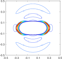
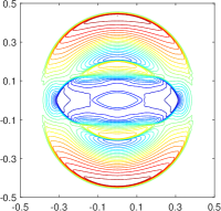
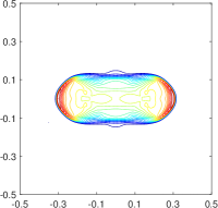
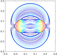
Figure 5: The contour plots of $\rho$, $p_{m}$, $p$, and $\|{\bm{v}}\|$ (from let to right) for the blast problem at $t=0.01$.

Example 7.1 (Blast problem).

This test simulates a benchmark MHD problem in the domain $[-0.5,0.5]^{2}$ with outflow boundary conditions. The setup is similar to that in [1] except for a fluid mixture with $n_{c}=2$, $C_{v_{1}}=2.42$, $C_{v_{2}}=0.72$, $\Gamma_{1}=5/3$, and $\Gamma_{2}=1.4$. Initially, the fluid is stationary, with $(\rho,p,Y_{1},Y_{2})=(1,1000,1,0)$ in the explosion region ($x^{2}+y^{2}\leq 0.01$) and $(1,0.1,0,1)$ in the ambient region ($x^{2}+y^{2}>0.01$). The magnetic field $\bf B$ is initialized as $(100/\sqrt{4\pi},0,0)$. Due to the large jump in $p$ and the strong magnetic field, negative numerical $p$ can be easily produced and often cause failure of the numerical simulations. Fig. 5 presents the contour plots of the density $\rho$, the magnetic pressure $p_{m}=\frac{1}{2}\|{\bf B}\|^{2}$, the thermal pressure $p$, and the velocity magnitude $\|{\bm{v}}\|$ computed by the proposed bound-preserving discontinuous Galerkin method with $400\times 400$ uniform cells. We observe the flow structures are well captured, and our method is highly robust and always preserves the bound principles Eq. 88 in the whole simulation.

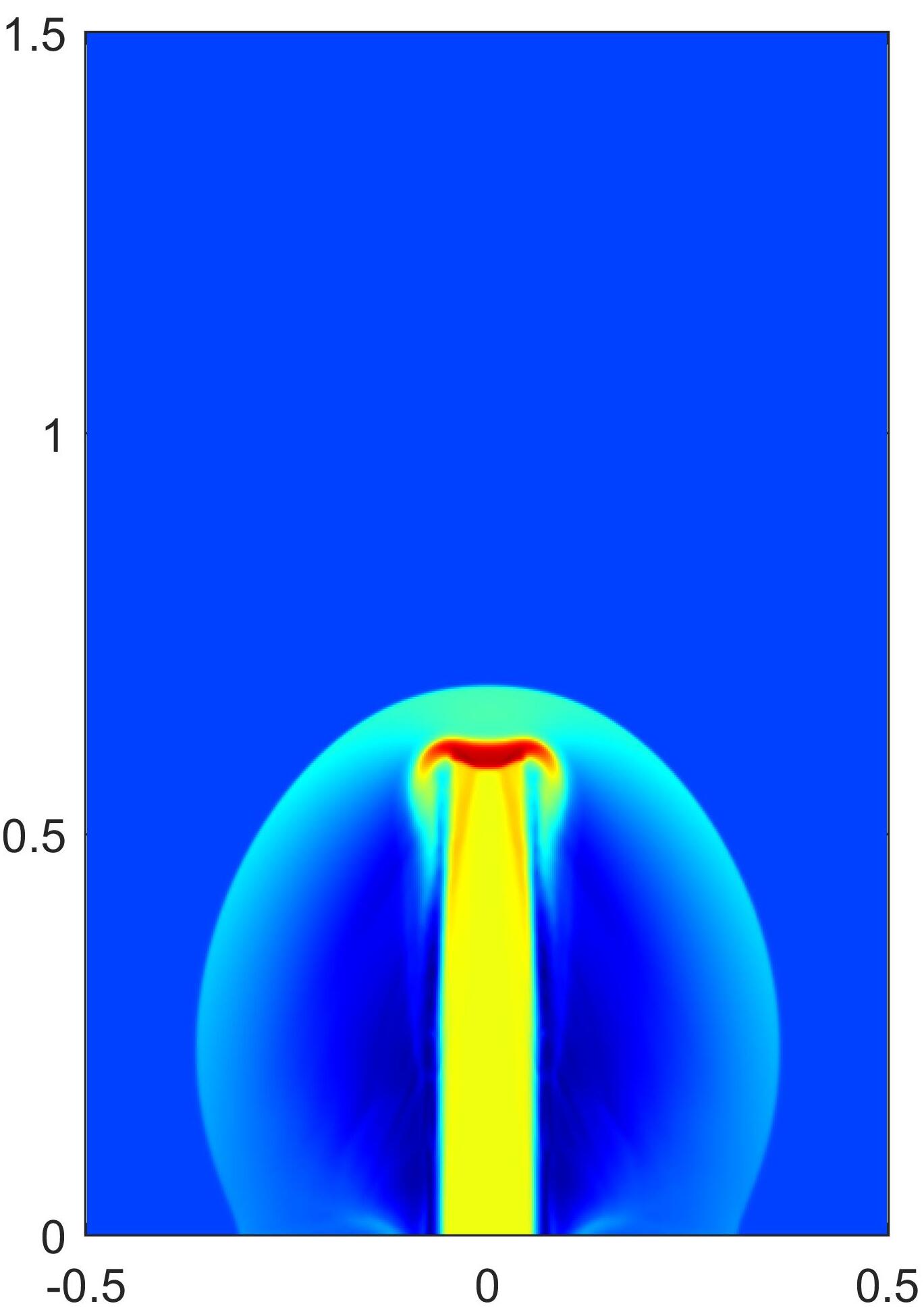
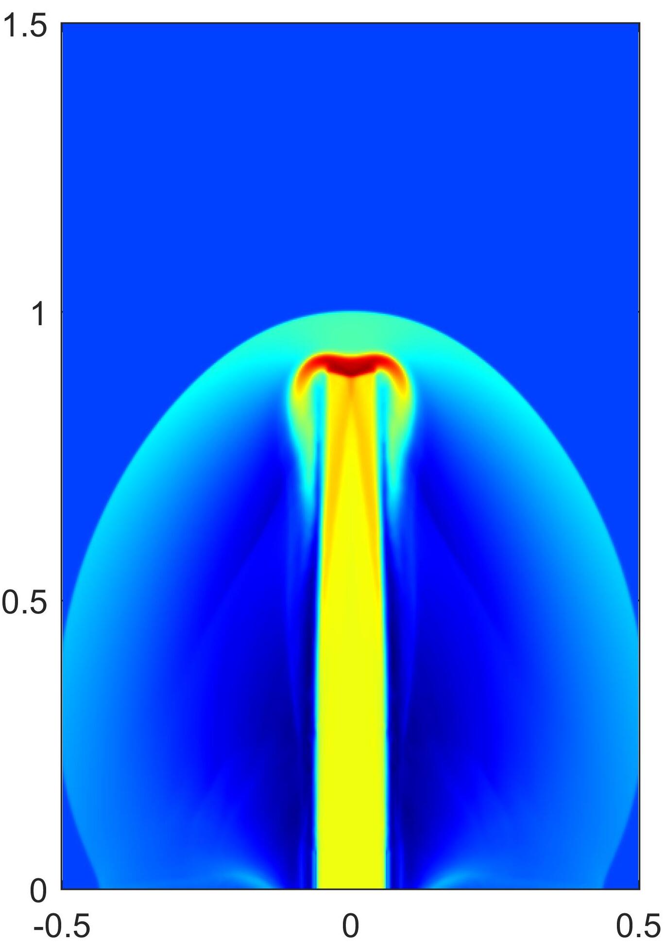
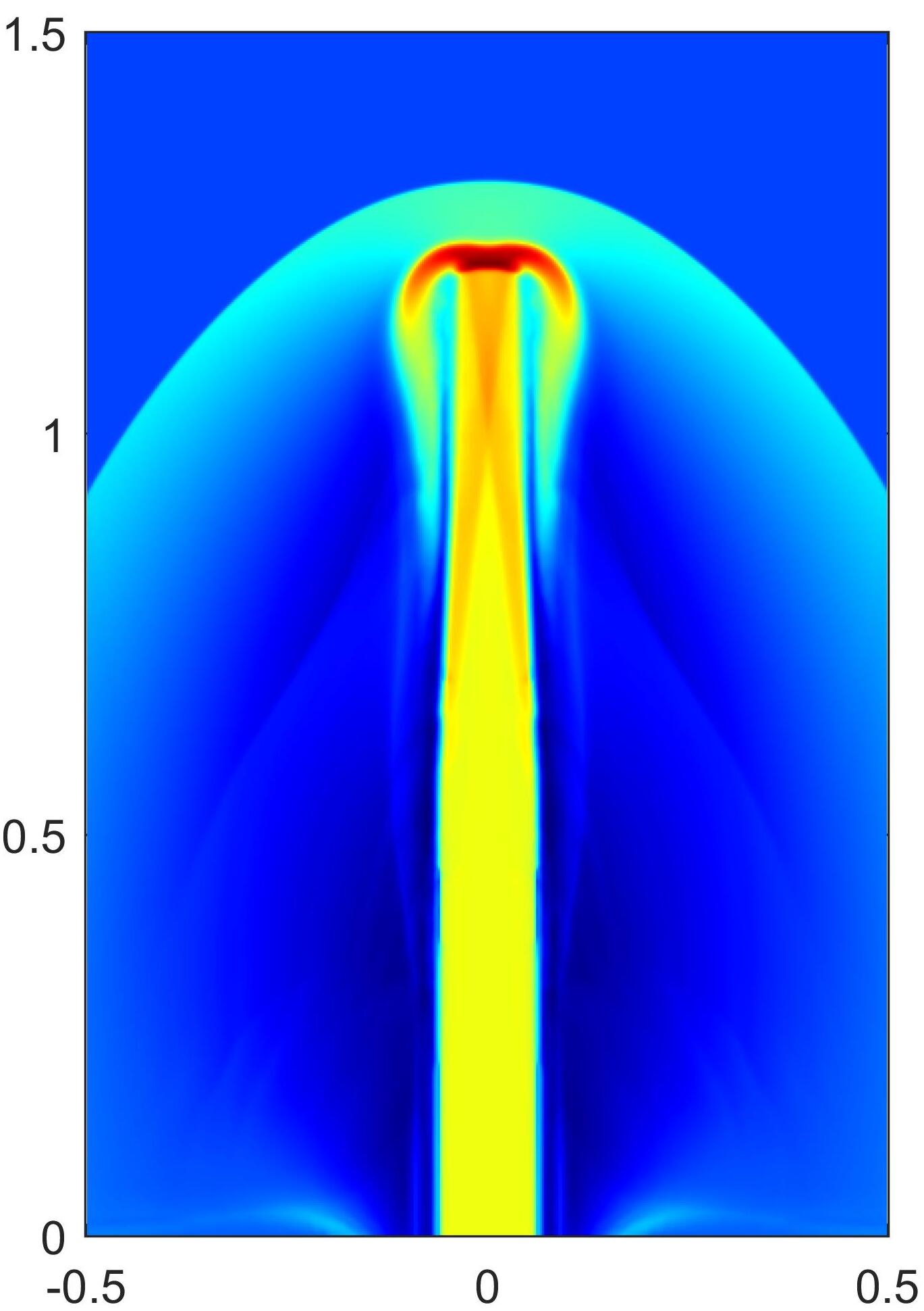
Figure 6: The plots of $\log(\rho)$ for the jet problem. From left to right: $t=0.001$, $0.0015$ and $0.002$.

Example 7.2 (Astrophysical jet).

This test simulates a high-speed MHD jet flow in the domain $[-0.5,0.5]\times[0,1.5]$ with $n_{c}=2$, $C_{v_{1}}=0.72$, $C_{v_{2}}=2.42$, $\Gamma_{1}=1.4$, and $\Gamma_{2}=5/3$. The domain is initially filled with static fluid with $(\rho,p,Y_{1},Y_{2})=(0.14,1,0,1)$. The inflow jet condition is fixed on boundary $\{|x|<0.05,y=0\}$ with $(\rho,p,Y_{1},Y_{2})=(1.4,1,1,0)$ and ${\bm{v}}=(0,800,0)$, while the outflow conditions are specified on the other boundaries. There is a strong magnetic field $\bf B$ initialized as $(0,\sqrt{4000},0)$, which makes this test more challenging. Our simulation is based on the proposed bound-preserving method with $200\times 600$ uniform cells in $[0,0.5]\times[0,1.5]$. The numerical results are shown Fig. 6. The flow pattern is captured with high resolution and similar to the single-component MHD case reported in [53, 54]. In such an extreme test, our bound-preserving method exhibits good robustness. However, if the proposed scaling limiter is not used to enforce (96), or if the locally divergence-free technique is not employed to ensure ${\rm div}_{ij}^{{-}}{\bf B}=0$, or if the proposed source term Eq. 106 is dropped, the resulting method even with the WENO limiter is not bound-preserving and would fail quickly due to nonphysical numerical solutions out of the bounds. This confirms our theoretical analyses and the importance of the proposed conditions and techniques.

8 Conclusions

We have systematically proposed a novel and general framework, called geometric quasilinearization (GQL), for studying bound-preserving problems with nonlinear constraints. GQL skillfully transfers all nonlinear constraints into linear ones, via properly introducing some free auxiliary variables independent of the system variables. We have established the fundamental principle and general theory of GQL, and provided three simple methods for constructing GQL representations. The GQL approach equivalently casts the nonlinear bound-preserving problems into preserving the positivity of linear functions, thereby opening up a new effective way for bound-preserving study. Several examples have been provided to demonstrate the effectiveness and advantages of the GQL approach in addressing nonlinear bound-preserving problems that are highly challenging and could not be easily handled by direct or traditional approaches. Besides the examples in this paper, recently the GQL approach also achieved successes in finding (high-order) bound-preserving schemes for several complicated PDE systems in [51, 53, 57, 52, 54, 55].

As the proposed GQL framework is not restricted to the specific forms of the PDEs, it applies to general time-dependent PDE systems that possess convex invariant regions with nonlinear constraints. Moreover, it can be used in conjunction with the well-developed limiters in [67, 68, 63, 23] to design high-order bound-preserving schemes. It can be expected the GQL approach will be useful for addressing more challenging bound-preserving problems for a variety of PDEs in the future.

Appendix A Proof of Theorem 3.8

The proof is divided into two steps.

(i) Prove that $G\subseteq G_{*}$. For any ${\bf u}_{*}\in\partial G$, the hyperplane $({\bf u}-{\bf u}_{*})\cdot{\bf n}_{*}=0$ supports the convex region $G$ at ${\bf u}_{*}$. Thus we have

(108) $$G\subseteq\{{\bf u}\in\mathbb{R}^{N}:\left({\bf u}-{\bf u}_{*},{\bf n}_{*}\right)\geq 0~{}~{}\forall{\bf u}_{*}\in\partial G\}.$$

If $G$ is closed, then Eq. 108 means $G\subseteq G_{*}$. Next, we assume $G$ is open and show $G\subseteq G_{*}$ by contradiction. Assume that

(109) there exists $${\bf u}_{0}\in G {\bf u}_{0}\notin G_{*}$$ but .

Then, according to Eq. 108, there exists ${\bf u}_{*}\in\partial G$ such that $({\bf u}_{0}-{\bf u}_{*})\cdot{\bf n}_{*}=0$. Since $G$ is open, there exists $\delta>0$ such that $\Omega_{\delta}:=\{{\bf u}\in\mathbb{R}^{N}:\|{\bf u}-{\bf u}_{0}\|<\delta\}\subset G$. We take ${\bf u}_{\delta}:={\bf u}_{0}-\frac{\delta}{2\|{\bf n}_{*}\|}{\bf n}_{*}\in\Omega_{\delta}.$ Then ${\bf u}_{\delta}\in G$. However, using $({\bf u}_{0}-{\bf u}_{*})\cdot{\bf n}_{*}=0$ gives

$$({\bf u}_{\delta}-{\bf u}_{*})\cdot{\bf n}_{*}=\left({\bf u}_{0}-{\bf u}_{*}-\frac{\delta}{2\|{\bf n}_{*}\|}{\bf n}_{*}\right)\cdot{\bf n}_{*}=-\frac{\delta}{2}\|{\bf n}_{*}\|<0,$$

which contradicts Eq. 108 and ${\bf u}_{\delta}\in G$. Thus the assumption Eq. 109 is incorrect, and we have $G\subseteq G_{*}$.

(ii) Prove that $G_{*}\subseteq G$. We first show that $G_{*}\subseteq{\rm cl}(G)$ by contradiction. Assume that

(110) there exists $${\bf u}_{0}\in G_{*} {\bf u}_{0}\notin{\rm cl}(G)$$ but .

According to the theory of convex optimization [5], the minimum of the convex function $\zeta({\bf u}):=\|{\bf u}-{\bf u}_{0}\|^{2}$ over the closed convex region ${\rm cl}(G)$ is attained at certain boundary point ${\bf u}_{*}\in\partial G$. Let $\widehat{\bf u}$ be an arbitrary interior point of $G$. Thanks to the convexity ${\rm cl}(G)$, one has ${\bf u}_{\lambda}:=\lambda\widehat{\bf u}+(1-\lambda){\bf u}_{*}\in{\rm cl}(G)$ for any $\lambda\in[0,1]$. We then know that the quadratic function

$$\widehat{\zeta}(\lambda):=\zeta({\bf u}_{\lambda})=\lambda^{2}\left\|\widehat{\bf u}-{\bf u}_{*}\right\|^{2}+2\lambda\left(\widehat{\bf u}-{\bf u}_{*}\right)\cdot\left({\bf u}_{*}-{\bf u}_{0}\right)+\|{\bf u}_{*}-{\bf u}_{0}\|^{2}$$

attains its minimum over $[0,1]$ at $\lambda=0$. This implies $\left(\widehat{\bf u}-{\bf u}_{*}\right)\cdot\left({\bf u}_{*}-{\bf u}_{0}\right)\geq 0$, for an arbitrary interior point $\widehat{\bf u}$ of $G$. Thus ${\rm int}(G)\subseteq\{{\bf u}:\left({\bf u}-{\bf u}_{*}\right)\cdot\left({\bf u}_{*}-{\bf u}_{0}\right)\geq 0\}=:H_{*}^{+}$, where $H_{*}^{+}$ is a closed halfspace. It follows that $H_{*}^{+}$ is a supporting halfspace to $G$, and ${\bf u}_{*}-{\bf u}_{0}$ is an inward-pointing normal vector of $G$ at ${\bf u}_{*}$. Because $\partial G$ is smooth, there exists $\mu>0$ such that ${\bf n}_{*}=\mu({\bf u}_{*}-{\bf u}_{0})$, which implies $({\bf u}_{0}-{\bf u}_{*})\cdot{\bf n}_{*}=-\mu\left\|{\bf u}_{0}-{\bf u}_{*}\right\|^{2}<0.$ This contradicts the assumption ${\bf u}_{0}\in G_{*}$. Thus the assumption Eq. 110 is incorrect, and we have $G_{*}\subseteq{\rm cl}(G)$. If $G$ is closed, then we obtain $G_{*}\subseteq G$. If $G$ is open, then $\partial G\cap G_{*}=\emptyset$, which along with $G_{*}\subseteq{\rm cl}(G)$ yields $G_{*}\subseteq G$.

In summary, we have $G=G_{*}$, and the proof is completed.

Appendix B A simple scaling limiter to enforce Eq. 96

The condition Eq. 96 is not always automatically satisfied by the polynomial vector ${\bf U}_{ij}^{n}(x,y)$ of the high-order schemes. If this happens, the following limiter is used to modify ${\bf U}_{ij}^{n}(x,y)$ into $\widetilde{\bf U}_{ij}^{n}(x,y)$ such that $\widetilde{\bf U}_{ij}^{n}(x,y)$ satisfies Eq. 96. Define $\mathbb{Q}_{ij}=\{(\widehat{x}_{i}^{(\beta)},y_{j}^{(q)}),(x_{i}^{(q)},\widehat{y}_{j}^{(\beta)})~{}\forall\beta,q\}$ as the set of all the points involved in Eq. 96. Since the limiter is performed separately for each cell, the subscripts $ij$ and superscript $n$ of all quantities are omitted below for convenience. First, modify the density as

$$\widehat{\rho}(x,y)=\overline{\rho}+\theta_{1}(\rho(x,y)-\overline{\rho}),\qquad\theta_{1}:=(\overline{\rho}-\epsilon_{1})/\big{(}\overline{\rho}-\min_{(x,y)\in\mathbb{Q}_{ij}}\rho(x,y)\big{)},$$

where $\epsilon_{1}$ is a small positive number and may be taken as $\min\{10^{-13},\overline{\rho}\}$. Define $\mathbb{S}_{k}=\{(x,y)\in\mathbb{Q}_{ij}:{\rho Y_{k}}(x,y)\leq 0\}$. Then, modify the mass fractions [13] as

$$\widehat{\rho Y_{k}}(x,y)={\rho Y_{k}}(x,y)+\theta_{2}\left(\frac{\overline{\rho Y_{k}}}{\overline{\rho}}\widehat{\rho}(x,y)-{\rho Y_{k}}(x,y)\right),\qquad 1\leq k\leq n_{c}-1,$$

where $\theta_{2}=\max_{1\leq k\leq n_{c}}\max_{(x,y)\in\mathbb{S}_{k}}\{\frac{-{\rho Y_{k}}(x,y)}{\overline{\rho Y_{k}}\widehat{\rho}(x,y)/\overline{\rho}-{\rho Y_{k}}(x,y)}\}$ with $\rho Y_{n_{c}}=\widehat{\rho}-\sum_{k=1}^{n_{c}-1}\rho Y_{k}$. Denote $\widehat{\bf U}=(\widehat{\rho{\bf Y}},\widehat{\rho},{\bm{m}},{\bf B},E)^{\top}$. Finally, modify $\widehat{\bf U}$ to enforce the positivity of $g({\bf U})=E-\frac{1}{2}({\|{\bm{m}}\|^{2}}/\rho+{\|{\bf B}\|^{2}})$ by

$$\widetilde{\bf U}(x,y)=\overline{\bf U}+\theta_{3}(\widehat{\bf U}(x,y)-\overline{\bf U}),\qquad\theta_{3}:=(g(\overline{\bf U})-\epsilon_{2})/\big{(}g(\overline{\bf U})-\min_{(x,y)\in\mathbb{Q}_{ij}}g(\widehat{\bf U}(x,y))\big{)},$$

where $\epsilon_{2}$ is a small positive number and may be taken as $\min\{10^{-13},g(\overline{\bf U})\}$. Note that the pressure function $p({\bf U})$ in Eq. 87 is generally not concave so we use the concave function $g({\bf U})$ instead of $p({\bf U})$. It can be verified that the limited solution $\widetilde{\bf U}(x,y)\in G$ for all $(x,y)\in\mathbb{Q}_{ij}$ and its cell average equals $\overline{\bf U}$. Such type of limiters do not lose the high-order accuracy, as demonstrated in [67, 68, 66].

References

- [1] D. S. Balsara and D. Spicer, A staggered mesh algorithm using high order Godunov fluxes to ensure solenoidal magnetic fields in magnetohydrodynamic simulations, J. Comput. Phys., 149 (1999), pp. 270–292.
- [2] P. Batten, N. Clarke, C. Lambert, and D. M. Causon, On the choice of wavespeeds for the HLLC Riemann solver, SIAM J. Sci. Comput., 18 (1997), pp. 1553–1570.
- [3] C. Berthon, P. Charrier, and B. Dubroca, An HLLC scheme to solve the M1 model of radiative transfer in two space dimensions, J. Sci. Comput., 31 (2007), pp. 347–389.
- [4] J. Borwein and A. S. Lewis, Convex Analysis and Nonlinear Optimization: Theory and Examples, Springer Science & Business Media, 2010.
- [5] S. Boyd, S. P. Boyd, and L. Vandenberghe, Convex Optimization, Cambridge University Press, 2004.
- [6] P. Chandrashekar, A global divergence conforming DG method for hyperbolic conservation laws with divergence constraint, J. Sci. Comput., 79 (2019), pp. 79–102.
- [7] J. Cheng and C.-W. Shu, Positivity-preserving Lagrangian scheme for multi-material compressible flow, J. Comput. Phys., 257 (2014), pp. 143–168.
- [8] Q. Cheng and J. Shen, Global constraints preserving scalar auxiliary variable schemes for gradient flows, SIAM J. Sci. Comput., 42 (2020), pp. A2489–A2513.
- [9] Y. Cheng, I. Gamba, and J. Proft, Positivity-preserving discontinuous Galerkin schemes for linear Vlasov-Boltzmann transport equations, Math. Comp., 81 (2012), pp. 153–190.
- [10] Y. Cheng, F. Li, J. Qiu, and L. Xu, Positivity-preserving DG and central DG methods for ideal MHD equations, J. Comput. Phys., 238 (2013), pp. 255–280.
- [11] A. J. Christlieb, Y. Liu, Q. Tang, and Z. Xu, High order parametrized maximum-principle-preserving and positivity-preserving WENO schemes on unstructured meshes, J. Comput. Phys., 281 (2015), pp. 334–351.
- [12] A. J. Christlieb, Y. Liu, Q. Tang, and Z. Xu, Positivity-preserving finite difference weighted ENO schemes with constrained transport for ideal magnetohydrodynamic equations, SIAM J. Sci. Comput., 37 (2015), pp. A1825–A1845.
- [13] J. Du, C. Wang, C. Qian, and Y. Yang, High-order bound-preserving discontinuous Galerkin methods for stiff multispecies detonation, SIAM J. Sci. Comput., 41 (2019), pp. B250–B273.
- [14] Q. Du, Z. Huang, and P. G. LeFloch, Nonlocal conservation laws. a new class of monotonicity-preserving models, SIAM J. Numer. Anal., 55 (2017), pp. 2465–2489.
- [15] Q. Du, L. Ju, X. Li, and Z. Qiao, Maximum bound principles for a class of semilinear parabolic equations and exponential time-differencing schemes, SIAM Review, 63 (2021), pp. 317–359.
- [16] P. Fu, F. Li, and Y. Xu, Globally divergence-free discontinuous Galerkin methods for ideal magnetohydrodynamic equations, J. Sci. Comput., 77 (2018), pp. 1621–1659.
- [17] S. K. Godunov, Symmetric form of the equations of magnetohydrodynamics, Numerical Methods for Mechanics of Continuum Medium, 1 (1972), pp. 26–34.
- [18] S. Gottlieb, C.-W. Shu, and E. Tadmor, Strong stability-preserving high-order time discretization methods, SIAM Review, 43 (2001), pp. 89–112.
- [19] P. M. Gruber, Convex and Discrete Geometry, vol. 336, Springer Science & Business Media, 2007.
- [20] J.-L. Guermond, M. Nazarov, B. Popov, and I. Tomas, Second-order invariant domain preserving approximation of the Euler equations using convex limiting, SIAM J. Sci. Comput., 40 (2018), pp. A3211–A3239.
- [21] J.-L. Guermond and B. Popov, Invariant domains and first-order continuous finite element approximation for hyperbolic systems, SIAM J. Numer. Anal., 54 (2016), pp. 2466–2489.
- [22] J.-L. Guermond and B. Popov, Invariant domains and second-order continuous finite element approximation for scalar conservation equations, SIAM J. Numer. Anal., 55 (2017), pp. 3120–3146.
- [23] X. Y. Hu, N. A. Adams, and C.-W. Shu, Positivity-preserving method for high-order conservative schemes solving compressible Euler equations, J. Comput. Phys., 242 (2013), pp. 169–180.
- [24] Y. Jiang and H. Liu, Invariant-region-preserving DG methods for multi-dimensional hyperbolic conservation law systems, with an application to compressible Euler equations, J. Comput. Phys., 373 (2018), pp. 385–409.
- [25] L. Ju, X. Li, Z. Qiao, and J. Yang, Maximum bound principle preserving integrating factor Runge–Kutta methods for semilinear parabolic equations, J. Comput. Phys., 439 (2021), p. 110405.
- [26] B. Khobalatte and B. Perthame, Maximum principle on the entropy and second-order kinetic schemes, Math. Comp., 62 (1994), pp. 119–131.
- [27] L. Krivodonova, J. Xin, J.-F. Remacle, N. Chevaugeon, and J. E. Flaherty, Shock detection and limiting with discontinuous Galerkin methods for hyperbolic conservation laws, Appl. Numer. Math., 48 (2004), pp. 323–338.
- [28] I. E. Leonard and J. E. Lewis, Geometry of Convex Sets, John Wiley & Sons, Hoboken, New Jersey, 2015.
- [29] F. Li and C.-W. Shu, Locally divergence-free discontinuous Galerkin methods for MHD equations, J. Sci. Comput., 22 (2005), pp. 413–442.
- [30] F. Li, L. Xu, and S. Yakovlev, Central discontinuous Galerkin methods for ideal MHD equations with the exactly divergence-free magnetic field, J. Comput. Phys., 230 (2011), pp. 4828–4847.
- [31] H. Li and X. Zhang, On the monotonicity and discrete maximum principle of the finite difference implementation of - finite element method, Numer. Math., 145 (2020), pp. 437–472.
- [32] J. Li, X. Li, L. Ju, and X. Feng, Stabilized integrating factor Runge–Kutta method and unconditional preservation of maximum bound principle, SIAM J. Sci. Comput., 43 (2021), pp. A1780–A1802.
- [33] C. Liang and Z. Xu, Parametrized maximum principle preserving flux limiters for high order schemes solving multi-dimensional scalar hyperbolic conservation laws, J. Sci. Comput., 58 (2014), pp. 41–60.
- [34] D. Ling, J. Duan, and H. Tang, Physical-constraints-preserving Lagrangian finite volume schemes for one-and two-dimensional special relativistic hydrodynamics, J. Comput. Phys., 396 (2019), pp. 507–543.
- [35] A. K. Meena, H. Kumar, and P. Chandrashekar, Positivity-preserving high-order discontinuous Galerkin schemes for ten-moment Gaussian closure equations, J. Comput. Phys., 339 (2017), pp. 370–395.
- [36] A. K. Meena, R. Kumar, and P. Chandrashekar, Positivity-preserving finite difference WENO scheme for ten-moment equations with source term, J. Sci. Comput., 82 (2020), pp. 1–37.
- [37] C. Niculescu and L.-E. Persson, Convex Functions and Their Applications, Springer, 2006.
- [38] E. Olbrant, C. D. Hauck, and M. Frank, A realizability-preserving discontinuous Galerkin method for the M1 model of radiative transfer, J. Comput. Phys., 231 (2012), pp. 5612–5639.
- [39] B. Perthame, Second-order Boltzmann schemes for compressible Euler equations in one and two space dimensions, SIAM J. Numer. Anal., 29 (1992), pp. 1–19.
- [40] B. Perthame and C.-W. Shu, On positivity preserving finite volume schemes for Euler equations, Numer. Math., 73 (1996), pp. 119–130.
- [41] T. Qin, C.-W. Shu, and Y. Yang, Bound-preserving discontinuous Galerkin methods for relativistic hydrodynamics, J. Comput. Phys., 315 (2016), pp. 323–347.
- [42] R. T. Rockafellar, Convex Analysis, Princeton University Press, 2015.
- [43] J. A. Rossmanith and D. C. Seal, A positivity-preserving high-order semi-Lagrangian discontinuous Galerkin scheme for the Vlasov–Poisson equations, J. Comput. Phys., 230 (2011), pp. 6203–6232.
- [44] J. Shen and J. Xu, Unconditionally bound preserving and energy dissipative schemes for a class of Keller–Segel equations, SIAM J. Numer. Anal., 58 (2020), pp. 1674–1695.
- [45] C.-W. Shu, Bound-preserving high-order schemes for hyperbolic equations: Survey and recent developments, in Theory, Numerics and Applications of Hyperbolic Problems II, C. Klingenberg and M. Westdickenberg, eds., Cham, 2018, Springer International Publishing, pp. 591–603.
- [46] M. Spivak, Calculus on Manifolds, W. A. Benjamin, New York, 1965.
- [47] E. Tadmor, A minimum entropy principle in the gas dynamics equations, Appl. Numer. Math., 2 (1986), pp. 211–219.
- [48] H.-Z. Tang and K. Xu, Positivity-preserving analysis of explicit and implicit Lax–Friedrichs schemes for compressible Euler equations, J. Sci. Comput., 15 (2000), pp. 19–28.
- [49] T. Tang and K. Xu, Gas-kinetic schemes for the compressible Euler equations: positivity-preserving analysis, Z. Angew. Math. Phys., 50 (1999), pp. 258–281.
- [50] K. Wu, Design of provably physical-constraint-preserving methods for general relativistic hydrodynamics, Phys. Rev. D, 95 (2017), 103001.
- [51] K. Wu, Positivity-preserving analysis of numerical schemes for ideal magnetohydrodynamics, SIAM J. Numer. Anal., 56 (2018), pp. 2124–2147.
- [52] K. Wu, Minimum principle on specific entropy and high-order accurate invariant region preserving numerical methods for relativistic hydrodynamics, SIAM J. Sci. Comput., in press (2021).
- [53] K. Wu and C.-W. Shu, A provably positive discontinuous Galerkin method for multidimensional ideal magnetohydrodynamics, SIAM J. Sci. Comput., 40 (2018), pp. B1302–B1329.
- [54] K. Wu and C.-W. Shu, Provably positive high-order schemes for ideal magnetohydrodynamics: analysis on general meshes, Numer. Math., 142 (2019), pp. 995–1047.
- [55] K. Wu and C.-W. Shu, Provably physical-constraint-preserving discontinuous Galerkin methods for multidimensional relativistic MHD equations, Numer. Math., 148 (2021), pp. 699–741.
- [56] K. Wu and H. Tang, High-order accurate physical-constraints-preserving finite difference WENO schemes for special relativistic hydrodynamics, J. Comput. Phys., 298 (2015), pp. 539–564.
- [57] K. Wu and H. Tang, Admissible states and physical-constraints-preserving schemes for relativistic magnetohydrodynamic equations, Math. Models Methods Appl. Sci., 27 (2017), pp. 1871–1928.
- [58] K. Wu and H. Tang, Physical-constraint-preserving central discontinuous Galerkin methods for special relativistic hydrodynamics with a general equation of state, Astrophys. J. Suppl. Ser., 228 (2017), 3.
- [59] K. Wu and Y. Xing, Uniformly high-order structure-preserving discontinuous Galerkin methods for Euler equations with gravitation: Positivity and well-balancedness, SIAM J. Sci. Comput., 43 (2021), pp. A472–A510.
- [60] Y. Xing, X. Zhang, and C.-W. Shu, Positivity-preserving high order well-balanced discontinuous Galerkin methods for the shallow water equations, Adv. Water Resour., 33 (2010), pp. 1476–1493.
- [61] T. Xiong, J.-M. Qiu, and Z. Xu, High order maximum-principle-preserving discontinuous Galerkin method for convection-diffusion equations, SIAM J. Sci. Comput., 37 (2015), pp. A583–A608.
- [62] T. Xiong, J.-M. Qiu, and Z. Xu, Parametrized positivity preserving flux limiters for the high order finite difference WENO scheme solving compressible Euler equations, J. Sci. Comput., 67 (2016), pp. 1066–1088.
- [63] Z. Xu, Parametrized maximum principle preserving flux limiters for high order schemes solving hyperbolic conservation laws: one-dimensional scalar problem, Math. Comp., 83 (2014), pp. 2213–2238.
- [64] Z. Xu and X. Zhang, Bound-preserving high-order schemes, in Handbook of Numerical Analysis, vol. 18, Elsevier, 2017, pp. 81–102.
- [65] D. Yuan, J. Cheng, and C.-W. Shu, High order positivity-preserving discontinuous Galerkin methods for radiative transfer equations, SIAM J. Sci. Comput., 38 (2016), pp. A2987–A3019.
- [66] X. Zhang, On positivity-preserving high order discontinuous Galerkin schemes for compressible Navier-Stokes equations, J. Comput. Phys., 328 (2017), pp. 301–343.
- [67] X. Zhang and C.-W. Shu, On maximum-principle-satisfying high order schemes for scalar conservation laws, J. Comput. Phys., 229 (2010), pp. 3091–3120.
- [68] X. Zhang and C.-W. Shu, On positivity-preserving high order discontinuous Galerkin schemes for compressible Euler equations on rectangular meshes, J. Comput. Phys., 229 (2010), pp. 8918–8934.
- [69] X. Zhang and C.-W. Shu, Positivity-preserving high order discontinuous Galerkin schemes for compressible Euler equations with source terms, J. Comput. Phys., 230 (2011), pp. 1238–1248.
- [70] X. Zhang and C.-W. Shu, A minimum entropy principle of high order schemes for gas dynamics equations, Numer. Math., 121 (2012), pp. 545–563.
- [71] X. Zhang, Y. Xia, and C.-W. Shu, Maximum-principle-satisfying and positivity-preserving high order discontinuous Galerkin schemes for conservation laws on triangular meshes, J. Sci. Comput., 50 (2012), pp. 29–62.
- [72] Y. Zhang, X. Zhang, and C.-W. Shu, Maximum-principle-satisfying second order discontinuous Galerkin schemes for convection–diffusion equations on triangular meshes, J. Comput. Phys., 234 (2013), pp. 295–316.
- [73] J. Zhao and H. Tang, Runge-Kutta discontinuous Galerkin methods for the special relativistic magnetohydrodynamics, J. Comput. Phys., 343 (2017), pp. 33–72.