Information-Theoretic Bias Assessment Of Learned Representations Of Pretrained Face Recognition

Abstract

As equality issues in the use of face recognition have garnered a lot of attention lately, greater efforts have been made to debiased deep learning models to improve fairness to minorities. However, there is still no clear definition nor sufficient analysis for bias assessment metrics. We propose an information-theoretic, independent bias assessment metric to identify degree of bias against protected demographic attributes from learned representations of pretrained facial recognition systems. Our metric differs from other methods that rely on classification accuracy or examine the differences between ground truth and predicted labels of protected attributes predicted using a shallow network. Also, we argue, theoretically and experimentally, that logits-level loss is not adequate to explain bias since predictors based on neural networks will always find correlations. Further, we present a synthetic dataset that mitigates the issue of insufficient samples in certain cohorts. Lastly, we establish a benchmark metric by presenting advantages in clear discrimination and small variation comparing with other metrics, and evaluate the performance of different debiased models with the proposed metric.

I Introduction

The social impact of deep learning has been under scrutiny with the recent rapid developments in many application domains, such as face recognition [37] being used in surveillance and security [42]. One of the major concerns is demographic bias of deep learning systems with respect to protected attributes, such as sex [6], race [31] or age [12]. The bias is reflected in the unequal algorithmic accuracy for different demographic groups, such that in facial recognition systems, black females are less likely to be correctly recognized than white males [6] and people of color tend to be mistakenly recognized than people of European origin [11]. Bias issues, hampering generalization for facial recognition systems, are in part due to the end-to-end nature of training deep learning systems, which primarily focuses on minimizing empirical loss in order to maximize recognition accuracy at the expense of encouraging the model to exploit the information from protected attributes.

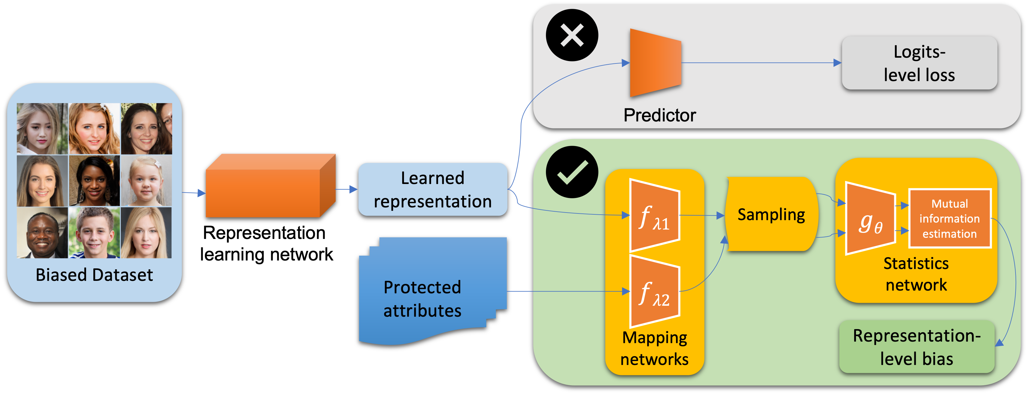
Figure 1: We propose an information-theoretic model to assess the bias involving protected attributes in facial recognition systems. Our approach directly establishes the correlation between learned representation $\mathcal{R}$ and protected attributes $\mathcal{Z}$ with mutual information without relying on any predictors at the logits level.

Mitigating bias, commonly referred to as debiasing in face recognition literature, has, therefore, garnered tremendous interest [28, 6, 40]. Without loss of generality, methods addressing algorithmic bias can be grouped into two families. First, a group of methods that attempt to mitigate bias by improving the diversity and inclusion of training datasets by resampling [28] or adding diversity [44, 38, 6]. Second, a group of methods that attempt to explicitly produce models that factor in protected attribute information to close the performance gap between different demographics [38, 15, 40].

Meanwhile, adopting a precise, universally applicable and acceptable metric for the degree of bias is both intrinsically difficult and important. Without loss of generality, three main approaches for bias assessment are based on either (1) classification accuracy across cohorts [2, 35, 38], (2) information leakage from protected attributes to prediction logits of labels [16, 45, 40], or (3) estimated correlations between prediction logits and protected attributes using shallow classifiers [28, 41, 20]. Classification accuracy-based bias assessment metrics may not be accurate because accuracy across cohorts must be listed and compared together. Moreover, information leakage-based methods, such as Demographic Parity, Equality of Odds, and Equality of Opportunity [16] strictly define fairness of a classification model as the independence between protected attributes and prediction logits of labels, which may not be appropriate to compare debiased models directly, as discussed in Section IV-A. Besides, quantitative metrics, relying on estimated correlations [18] using a shallow predictor, may find correlations even in unbiased data and would then mistakenly identify them as biased, as discussed in Section IV-B. Further, most of proposed bias assessment metrics are rarely used to evaluate other debiased models, as a mean to show universality. To the best of our knowledge, there is no universal way to assess the degree of bias for existing debiased models as these models have been evaluated on different benchmarks under varying conditions.

Prior work [2, 15, 38] mainly focus on bias mitigation instead of bias assessment, particularly neglecting representation/embedding level bias. Therefore, we propose an effective representation-level method to assess the demographic bias of any pretrained backbone (possibly debiased) facial recognition systems and design a series of experiments as a protocol to validate the rationality and effectiveness of bias assessment metrics in face recognition. We use entropy to assess dataset bias and mutual information to assess model bias from learned representation extracted by backbone models, rather than simply establishing correlations by training a shallow predictor using logits, as illustrated in Fig. 1. We combine dataset bias and representation-level model bias to comprehensively assess the percentage of remaining bias after a debiased backbone model, given the overall dataset bias. In other words, large remaining bias represents inferior debiasing performance. In this respect, our method can also help assess the bias using representations/embeddings in a layer-by-layer fashion inside any model. The proposed metric is not intended to be combined with other debiasing methods, but to actually independently evaluate debiasing methods as shown in Section V-E. The effectiveness of our method is verified with experiments on Colored MNIST [26], FairFace [21], CelebA [29] and synthetic datasets generated by StyleGAN2 [23]. Our key contributions can be summarized as follows:

• Theoretical and empirical arguments that bias assessment should be applied at the representation level instead of the logits level.

• An independent bias assessment metric at the representation level to help study bias mitigation.

• A performance evaluation for a wide range of debiasing techniques using the proposed independent metric.

• A synthetic dataset that mitigates the issue of insufficient samples in certain subsets.

• A categorization of different bias metrics.

II Related work

Protected attributes. Protected attributes are qualities, traits or characteristics that, by law, cannot be discriminated against [33]. Many studies [7, 36, 14] show that facial recognition systems have divergent recognition accuracy for different demographic groups. Meanwhile, using existing datasets [29, 30], which are dominated by sufficient samples in specific racial or sex groups, may also lead to unfairness against specific such groups.

Debiasing face recognition. The fairness of face recognition may be dramatically impacted by the bias issues in existing datasets in terms of the long-tail distribution [46] of demographic groups. To address bias issues, some studies introduce fairness into face recognition to mitigate demographic bias. The mainstream debiasing models belong to either (1) strategic sampling method [28] via oversampling or re-weighting to keep the training data balanced across cohorts, (2) representation disentanglement methods [12, 2, 19] to remove the specific demographic attribute by adversarial training, (3) domain adaptation methods [38, 15] for learning demographic-group invariant representations by maximizing the recognition performance of identity and minimizing the capability to predict protected attributes using a discrimination loss, or (4) domain independent training method [40] by learning an ensemble that constitutes separate classifiers per demographic group with representation sharing.

Bias assessment metrics. While many debiased models have been developed for face recognition, there has been limited progress in establishing an objective, quantitative and universally acceptable bias assessment metric. In particular, most of bias assessments rely on cross-cohort-terms based on classification accuracy [2], False Positive Rate (FPR) [43], Receiver Operating Characteristic (ROC) [15] and Area under the ROC Curve (AUC) [38]. Besides, information leakage from protected attributes to predicted labels has also been used to assess bias. For example, Demographic Parity, Equality of Odds, and Equality of Opportunity [16] use independence between protected attributes and prediction logits of labels to define fairness. Likewise, the difference between dataset leakage (i.e. the predictability of sex from ground truth labels) and model leakage (i.e. the predictability of sex from model predictions) [39] have also been used to assess the bias. Similarly, bias amplification [45] is defined as the difference of bias score (i.e. the percentage of occurrences of a given outcome and a demographic variable in the corpus) between training data and testing data. Moreover, several bias assessment metrics based on the estimated correlation using a shallow network at the logits level have been proposed. For example, dataset bias [28, 27] captures the bias of a dataset, measured by the classification performance with the cross entropy loss. More generally, the metric used in [41, 20] assesses bias based on prediction logits to predict protected attributes from representations. However, all aforementioned metrics are implicitly or explicitly based on accuracy or logits loss after the predictor at the logits level instead of the representation/embedding level, and therefore we call them logits-level bias assessment metrics.

Distance correlation $dcor^{2}$ [34] has been used to assess the bias at the representation level in [1] . However, in [1], the usage of distance correlation only considers model bias from the representations without a correction of dataset bias if the distribution of protected attributes varies as discussed in Section V-B, and yields more variation than our proposed metric as discussed in Section V-E.

III Representation-Level Bias Assessment

As discussed in Section II, most of the existing bias assessment methods depend on training shallow predictors that could overfit to spurious correlations between the input data and protected attributes, as illustrated in Fig. 1. Our goal is therefore to develop an independent (i.e. method-agnostic) bias assessment metric which can be applied at the representation/embedding level of pretrained (possibly debiased) models, and considers training dataset bias.

Consider a face recognition task for which, given a dataset $\mathcal{D}$ containing instances $(x_{i},y_{i},z_{i})$, where $x_{i}\in\mathcal{X}$ is an image annotated with a set of task-specific labels $y_{i}\in\mathcal{Y}$ (e.g. identity), and other protected attributes $z_{i}\in\mathcal{Z}$ (e.g. sex), the representation learning network $F_{\theta}:\mathcal{X}\to\mathcal{R}$ parametrized by $\theta\in\Theta$ first produces a learned representation $r_{i}\in\mathcal{R}$, and then a classifier $C_{\phi}:\mathcal{R}\to\mathcal{Y^{\prime}}$ with parameters $\phi\in\Phi$ produces the predicted label $y^{\prime}_{i}\in\mathcal{Y^{\prime}}$. The learned representation $r_{i}\in\mathcal{R}$ produced by representation learning sub-network $F_{\theta}$ may contain information about $z_{i}$, due to the end-to-end nature of training, which encourages models to exploit any information (including protected attributes) if it leads to lower empirical loss. Demographic parity (DP) [16] seeks to find information leakage between $\mathcal{Z}$ and $\mathcal{Y^{\prime}}$.

Definition 1: DEMOGRAPHIC PARITY. A classification model $\hat{T}$ is said to satisfy demographic parity if predicted label $Y^{\prime}=\hat{T}(X)$ and protected attribute $Z$ are independent.

However, DP does not completely ensure fairness [10] since the logits-level parity can arise naturally when there is little training data for one protected attribute $z_{i}$, and may impair the achievable utility of better classification accuracy since some correct predictions may contradict DP in general if the testing dataset is not strictly balanced, which will be further elaborated in Section IV-A. In order to overcome these drawbacks, we therefore propose:

Definition 2: REPRESENTATION-LEVEL DEMOGRAPHIC PARITY. A classifier $\hat{T}$ is said to satisfy representation-level demographic parity if learned representation $\hat{R}=\hat{F}(X)$ and protected attribute $Z$ are independent.

Representation-level demographic parity means that for all values of the protected attributes $Z$: $P(\hat{F}(X)=\hat{r})=P(\hat{F}(X)=\hat{r}|Z=z)$ where $\hat{F}$ is a representation learning sub-network. Mutual information (MI) which is widely used in representation disentanglement and debiasing [38, 24, 32], is then a natural approach for assessing the mutual dependence between $\mathcal{R}$ and $\mathcal{Z}$, and produce an information-theoretic fairness score. Independence is achieved when the representation space $\mathcal{R}$ contains no information about protected attributes $\mathcal{Z}$. More generally, we can say that $B\propto I(R,Z)$, where $B$ is the representation-level bias and $I$ is mutual information.

Facial recognition bias [37] stems from a biased trained model $T_{biased}$ and/or an imbalanced training dataset $\mathcal{D}_{biased}$. Representation-level bias reveals the degree of bias for the model $T_{biased}$ reflected in the learned representation $R$ extracted by the feature extraction sub-network $F$ inside $T_{biased}$. We use mutual information between $R$ and $Z$ to estimate the representation-level bias for the biased trained model $T_{biased}$, i.e. $I(R,Z)$. Furthermore, since a more imbalanced training dataset leads to more bias in the trained model, we use the entropy of $Z$ to assess the imbalance of the dataset $\mathcal{D}_{biased}$, i.e. $H(Z)$. Greater entropy implies a more balanced dataset. Therefore, we define the representation-level bias as follows.

Definition 3: REPRESENTATION-LEVEL BIAS (RLB). The representation-level bias $B$ of a classification model $T$ trained with a dataset $\mathcal{D}$, with respect to protected attribute $Z$, is defined as,

$$B(R,Z)=\frac{I(R,Z)}{H(Z)},$$ (1)

where $H(Z)$ is the entropy of $Z$, estimated empirically by:

$$H(Z)=-\frac{1}{|\mathcal{Z}|}\sum_{z\in\mathcal{Z}}\log{P_{z}},$$ (2)

and $I(R,Z)$ is the mutual information between $R$ and $Z$, estimated based on Definition 3.1 in  [5]:

$$I(R,Z)=\sup_{\theta\in\Theta}\mathop{{}\mathbb{E}_{\mathbb{P}_{\mathcal{RZ}}}}[T_{\theta}]-\log(\mathop{{}\mathbb{E}_{{\mathbb{P}_{\mathcal{R}}\otimes{\mathbb{P}_{\mathcal{Z}}}}}}[e^{T_{\theta}}]),$$ (3)

which estimates MI by training a neural network $T_{\theta}$ to distinguish between joint samples $\mathbb{P}_{\mathcal{RZ}}$ and the product of marginals $\mathbb{P}_{\mathcal{R}}\otimes\mathbb{P}_{\mathcal{Z}}$, of random variables $R$ and $Z$. The ratio $B$ is bounded ($[0,1]$) and easy to interpret, rather than the uncertain and negative range for mutual information minus entropy (since entropy is greater than mutual information). Mutual information neural estimation (MINE) [5] offers a lower-bound based on the Donsker-Varadhan representation [9] of KL-divergence.

We improve the mutual information estimate of  [5] by adding a mapping network followed by the statistics network to improve the robustness. Given a pair of $(r,z)\in(\mathcal{R},\mathcal{Z})$, the non-linear mapping networks $f_{\lambda_{1}}:\mathcal{R}\to\mathcal{W}$ and $f_{\lambda_{2}}:\mathcal{Z}\to\mathcal{S}$ first produce $w\in\mathcal{W}$ and $s\in\mathcal{S}$. The mapping networks $f_{\lambda_{1}}$ and $f_{\lambda_{2}}$ are implemented using one fully connected layer with parameters $\lambda_{1}$ and $\lambda_{2}$. Input dimensionality are adapted with $(\mathcal{R},\mathcal{Z})$ and output dimensionality is kept same. Then, $k$ minibatch samples are draw from the joint distribution, i.e. $(w^{J}_{1},s^{J}_{1}),...,(w^{J}_{k},s^{J}_{k})\sim\mathbb{P}_{\mathcal{WS}}$. Similarly, we keep the same $k$ samples from the marginal distribution $\mathbb{P}_{\mathcal{S}}$, i.e. $s^{J}_{1},..,s^{J}_{k}\sim\mathbb{P}_{\mathcal{S}}$, and draw $k$ samples from the marginal distribution $\mathbb{P}_{\mathcal{W}}$, i.e. $w^{M}_{1},..,w^{M}_{k}\sim\mathbb{P}_{\mathcal{W}}.$ The statistics network $g_{\theta}:\mathcal{W}\times\mathcal{Z}\to\mathbb{R}$ parametrized by $\theta\in\Theta$ is designed to evaluate the lower-bound of mutual information as a real number. Mutual information approximation is estimated by,

$$I_{\theta}(W,S)=\frac{1}{k}\sum_{i=1}^{k}o^{J}_{i}-\log(\frac{1}{k}\sum_{i=1}^{k}e^{o^{M}_{i}}),$$ (4)

where

$$o^{J}_{i}=g_{\theta}(w^{J}_{i},s^{J}_{i}),\quad\textrm{and}\quad o^{M}_{i}=g_{\theta}(w^{M}_{i},s^{J}_{i}).$$ (5)

In each training iteration, the gradient propagates through the statistics and the mapping networks, and the parameters $[\lambda_{1},\lambda_{2},\theta]$ are updated by the gradient of loss function

$$\begin{split}L=-(\overline{O}^{J}_{i}-\frac{\overline{O}^{M}_{i}}{EMA^{M}_{t}}),\end{split}$$ (6)

where $EMA^{M}_{t}$ is the exponential moving average (EMA) of marginal sample outputs, i.e.

$$\begin{split}EMA^{M}_{t}=\left\{\begin{array}[]{lr}\overline{O}^{M}_{t},&t=0\\ \alpha\overline{O}^{M}_{t}+(1-\alpha)\overline{O}^{M}_{t-1},&t>1\\ \end{array}\right.\end{split}$$ (7)

where $\overline{O}^{M}_{t}$ is the moving average at iteration $t$ and $\alpha$ is smoothing coefficient. We optimize by simultaneously estimating and maximizing the mutual information until convergence as follows:

$$I(R,Z)=\max_{\theta\in\Theta}I_{\theta}(W,S).$$ (8)

Finally, Representation-Level Bias (RLB) $B(R,Z)$ can be given according to Def. 3.

IV Comparing Bias Assessment Metrics

TABLE I: Taxonomy of different bias metrics.

Taxonomy	Usage	Examples
Accuracy across cohorts	$R,Y$	Standard deviation of accuracy [3, 13], other metrics across cohorts (ROC [15], AUC [38], F1 score [1]).
Information leakage	$Z,Y^{\prime}$	Demographic Parity, Equality of Odds, Equality of Opportunity [16], Dataset leakage, Model leakage [39], Bias amplification [45].
Estimated correlation	$R,Z$	Dataset bias [28], logits-level loss [20, 41].
Statistical dependence	$R,Z$	Distance Correlation [34], Representation-Level Bias (RLB).

Having introduced RLB, we will theoretically discuss the advantages of RLB compared to several representative bias assessment metrics at the logits level. Table I summarizes the comparison.

IV-A Information Leakage Fairness Criterion

Information leakage-based metrics assess bias by measuring information leakage from $\mathcal{Z}$ to $\mathcal{Y^{\prime}}$. For example, Demographic Parity, Equality of Odds, and Equality of Opportunity [16] use independence between protected attributes $\mathcal{Z}$ and prediction logits of labels $\mathcal{Y^{\prime}}$, which are commonly used as the strict definition of fairness for data-driven classification models. Demographic parity (DP) requires the classification to be independent of protected attributes. Specifically, besides the predictor $P$ estimating $Y$ as accurately as possible, an additional adversarial network $G$ is introduced to predict a value for $Z$ from $Y^{\prime}$. DP is achieved when limiting any information about $Z$ leaking to $Y^{\prime}$. However, as argued in [10], DP has two limitations. First, the fairness may not be completely ensured under DP since the logits-level parity can arise naturally with little training data of $z_{i}$. By contrast, representation-level DP does not arise naturally since it is an ideal criterion which requires independence of high-dimensional learned representations and protected attributes, which is naturally unattainable in practice. Further, in contrast to $Z$, $R$ are high dimensional vectors with much higher capacity to tolerate noise than predicted labels $Y^{\prime}$ in original demographic parity. Second, DP may harshly forbid some correct predictions if they violate the criterion in general, which hinders achievable better classification accuracy. The failure case of pursuing DP is that some correct predictions may be forced to be incorrect since DP requires strict probability equality across cohorts. Further, compared to the harsh DP, RLB is a soft metric.

IV-B Correlation Estimation

Correlation estimation-based metrics assess bias by estimating the correlation between $\mathcal{R}$ and $\mathcal{Z}$ using a shallow network. As mentioned in [41, 20] to assess model bias by logits-level loss, they try to estimate the correlation by training a mapping $M$ from the family of shallow predictors $P_{\psi}$ parametrized by $\psi\in\Psi$ such that $Z^{l}\approx M(R^{k})$, where $M\in\{P_{\psi}\}_{\psi\in\Psi}$, $R^{k}$ is the learned representation with dimension $k$ and $Z^{l}$ is the protected attributes with dimension $l$ $(l<k)$. Model bias can then be assessed at the logits level by minimizing the loss or maximizing prediction accuracy from the predictor $P_{\hat{\psi}}$ that learns to predict $\mathcal{Z}$ from $\mathcal{R}$, with parameters $\hat{\psi}$ such that

$$\hat{\psi}=\underset{\psi\in\Psi}{\operatorname{arg\,min}}~{}Loss(P_{\psi}(R^{k}),Z^{l}).$$ (9)

However, this correlation is unstable and capricious since, the predictor $P_{\hat{\psi}}$ with parameters $\hat{\psi}$ is easily trained as a projection from $\mathcal{R}^{k}$ to $\mathcal{Z}^{l}$, i.e. from a high dimensional space to a low dimensional space.

Furthermore, we may arbitrarily construct a spurious or uncorrelated representation space $\tilde{\mathcal{R}}^{k}$ with the same dimension $k$ as real representation space $\mathcal{R}^{k}$ to confuse the shallow network $P_{\psi}$, as shown in Section V-A. The confused shallow network may also find a correlation between $\tilde{\mathcal{R}}^{k}$ and $\mathcal{Z}^{l}$ such that $Z_{i}^{l}\approx\tilde{M}(\tilde{R}^{k}_{i})$, where $\tilde{M}\in\{P_{\psi}\}_{\psi\in\Psi}$. Unfortunately, the spurious mapping $\tilde{M}$ would offer a minimum loss or a maximum prediction accuracy as the degree of bias even for the uncorrelated representation and protected attributes.

By contrast, the principal idea of RLB is that the correlation between $\mathcal{R}$ and $\mathcal{Z}$ should be independently estimated by mutual information, instead of a neural network in [41, 20]. The drawback that an auxiliary neural network in logits-level loss may produce spurious correlations is addressed by mutual information lower-bound estimation, for which consistency of the Donsker-Varadhan representation and the network parameters choice over $\{\theta\in\Theta\}$ for MI supremum in (3) are proved in [5]. The limitation of logits-level loss using a neural network predictor is a preconceived latent assumption that the correlation is determined by a mapping $M$ as a neural network with a specific architecture and parameters, such that $Z^{l}\approx M(R^{k})$ where $M=\{P_{\psi}\}_{\psi\in\Psi}$. By contrast, using mutual information, we do not care about what the mapping $M$ is explicitly so that we can relax the mapping $M$ of $\mathcal{Z}$ from $\mathcal{R}$ without regarding it as a specific neural network. Furthermore, the neural network in RLB initializes with the lowest estimated bias, and in each iteration, strives to increase it by exhaustively traversing different mapping functions $T_{\theta}$, as shown in Fig. 3(a). The curve eventually converges to the greatest estimated bias which is approximately the lower bound of the actual bias, which explains the fact that, in Table II, the estimated bias stays at the lowest point with synthesized representations. Contrastively, there is no lower-bound guarantee for the logits-level metrics based on the prediction accuracy or logits loss so that it may exceed the actual bias.

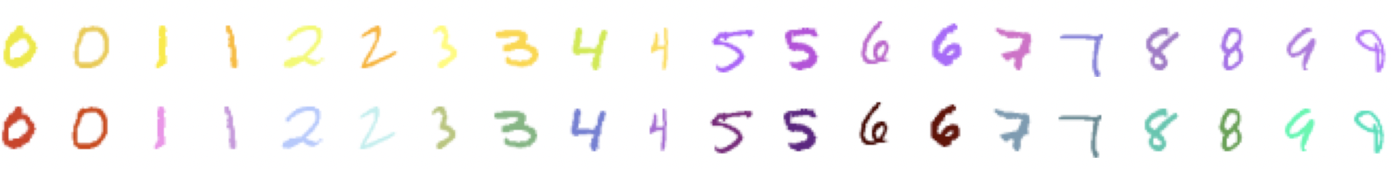
Figure 2: Examples of Colored MNIST, moderately biased (top) and extremely biased (bottom).

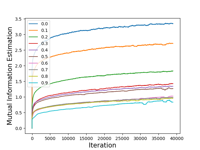
(a) Convergence lines of mutual information estimation.

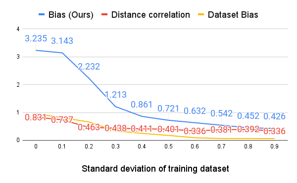
(b) Bias assessment of testing dataset with different standard deviations.

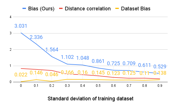
(c) Bias assessment of testing dataset with the fixed standard deviation.

Figure 3: Verification experiments on Colored MNIST Dataset.

V Experimental Evaluation

Prior work [44, 38, 6] argues that any bias assessment metrics must be capable of evaluating both dataset (im)balance and model bias. Therefore, we empirically demonstrate that our independent bias assessment metric at the representation level is more effective than other bias assessment metrics at the logits level in these two aspects with experiments on (1) Colored MNIST [26], (2) FairFace [21], (3) CelebA [29], and (4) synthetic datasets generated by StyleGAN2 [23]. First, a number of synthesized representations are used to test the robustness of our method compared to the estimated-correlation metrics, i.e. logits-level loss [41, 20] in Section V-A. Second, we verify that our method outperforms another estimated-correlation metric, i.e. dataset bias [27, 28] and a statistical-independence metric, i.e. distance correlation ${dcor}^{2}$ [34] by showing different bias scores for imbalanced datasets in Section V-B and reflecting the model bias at the representation level, which is further demonstrated in Section V-C and Section V-D. Finally, we show that RLB is generic and capable of evaluating different debiased models compared to the methods based on accuracy across cohorts, information leakage, i.e. bias amplification (BA) [45] and statistical dependence, i.e. ${dcor}^{2}$ [34] in Section V-E.

V-A Robustness Against Spurious Correlations

To verify the robustness of RLB and show that correlations could be found between both true or spurious protected attributes and both true or spurious representations, we introduce several synthesized representations using the Aligned & Cropped subset of CelebA dataset [29] since the learned representations extracted from cropped images focus more on demographic appearances (e.g. hair type, colors) and avoid the interference from other features (clothes). First, we train a ResNet-50 [17] to recognize attributes on CelebA dataset and use the qualified network $F$ to construct learned representation space $\mathcal{R}$. Then, we introduce several synthesized representations, including (1) $R_{S}$, shuffling learned representation over the feature dimension; (2) $R_{G}$, generating unpaired representations from a different but same-sample-size batch; (3) $Z_{S}$, shuffling protected attributes over the samples; and (4) $Z_{G}$, generating unpaired but overall-entropy-unchanged protected attributes labels, to confuse the bias assessment metric based on logits-level loss.

In Table II, we compare the proposed RLB with the logits-level loss (estimated-correlation metric) for sex bias. The results show that the correlations exist whether or not the synthesized representations are applied. There is no discrimination capability for testing prediction accuracy since several accuracy with synthesized representations approximate or exceed the accuracy without synthesized representations. Furthermore, the logits loss with synthesized representations is expected to be at least greater than that without synthesized representations since the spurious representation space $\tilde{\mathcal{R}}^{k}$ is fabricated at random and should be uncorrelated to protected attributes space $\mathcal{Z}^{l}$. However, the logits-level loss is crude to construct spurious correlations between unrelated samples. On the other hand, as we add spurious correlations, RLB declines, which means the correlation constructed by mutual information only exists between $\mathcal{R}$ and $\mathcal{Z}$ instead of any spurious representation space.

TABLE II: Comparison between correlations established by predictor and mutual information.

	Normal	$R_{S}$	$R_{G}$	$Z_{S}$	$Z_{G}$
	Correlation
Testing Acc.	99.7	63.8	99.9	92.3	99.8
Logits Loss	0.054	0.412	0.23e-05	0.179	0.026
Bias (Ours)	0.874	2.42e-05	0.34e-05	1.28e-05	1.09e-05

V-B Colored MNIST

To obtain intuitive insights and demonstrate the effectiveness of RLB for evaluating the (im)balance of training datasets and capturing dataset bias, we conduct experiments on a modified version of MNIST [26], Colored MNIST, where assigned colors are sampled from digit-dependent distributions. Since the digits are tied up with the colors, color classification can facilitate digit classification; and therefore, Colored MNIST is biased with color representations and the intensity can be controlled by the color assignment scheme. The moderately biased case (assigning two colors to two groups of digits) and extremely biased case (assigning ten distinct colors to each digit) are shown in Fig. 2.

Experiment Setup. We introduce color bias by assigning RGB colors $z_{i}=(r_{i},g_{i},b_{i})$ to each digit as the center color and provide a standard deviation (STD) $\sigma$ as its range; therefore, the color spectrum covered by each digit is $(r_{i}\pm\sigma,g_{i}\pm\sigma,b_{i}\pm\sigma)$. Increasing the STD $\sigma$ reduces bias since a larger STD will produce more overlap between the colors of different categories, thereby reducing the discriminability of colors. We train a LeNet-5 CNN [25] to recognize digits on Colored MNIST training set with different STDs $\sigma_{train}^{(i)}$ and use the qualified representation learning networks $F_{\sigma_{train}^{(i)}}$ to construct learned representation space $\mathcal{R}$ for representation-level bias assessment usage on the testing set with both different STDs $\sigma_{test}^{(i)}$ but same with training data and a fixed STD $\sigma_{test}=0.5$. Experiments with different STDs in testing data demonstrate that our method reflects the degree of bias in dataset, and other experiments with a fixed STD verify that the estimation of mutual information reflects bias in the trained model since the color entropy of the testing data is same, i.e. the denominator in (1) is same and the bias issues can only come from different biased models trained with different STDs.

Results. Fig. 3(a) shows that MI estimation, for a training dataset with different STDs and a testing dataset with a fixed STD, converge as several straight lines. Fig. 3(b) shows that in the case that the STD of training and testing datasets are similar, both dataset bias [28] and RLB decrease as the STD increases. However, ${dcor}^{2}$ does not yield this trend in high STD since it only considers model bias without a correction of dataset bias. In Fig. 3(c), the decrease of dataset bias [28] with the increase of STD does not happen with a fixed STD $\sigma_{test}$, and in nature it only assesses the bias from testing dataset with $\sigma_{test}=0.5$. On the other hand, the bias in the trained model is reflected in the representations of the testing dataset and captured by RLB as increase of the STD $\sigma_{train}$ of training dataset reduces RLB.

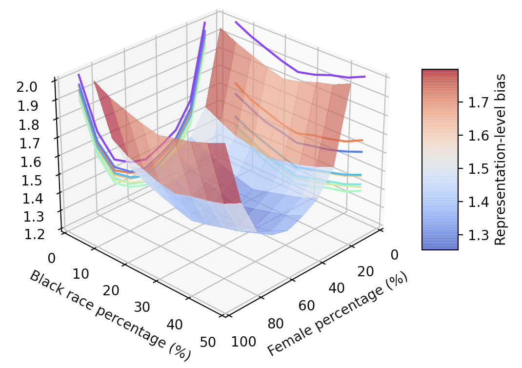
(a) Sampled FairFace datasets.

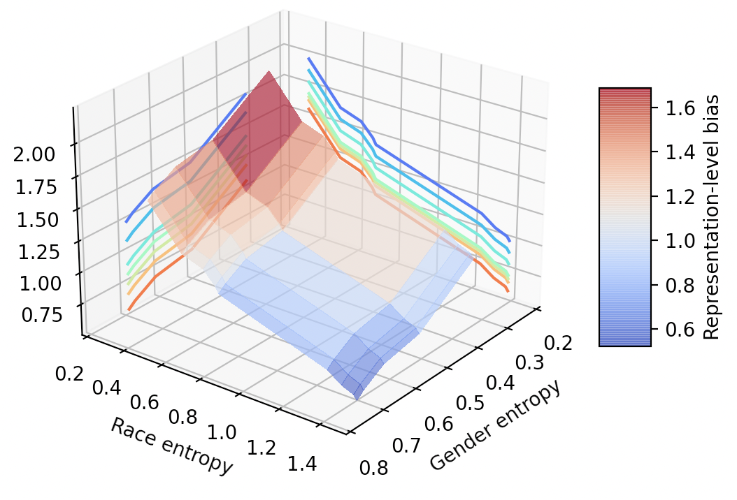
(b) Synthetic datasets.

Figure 4: Representation-level bias for sex and race.

V-C FairFace Dataset

Sampled datasets from FairFace dataset [21] are used to assess the bias induced by imbalanced datasets and explain the discrepancy due to imbalanced training [2, 37].

Experiment Setup. We emulate sex and racial bias by controlling female percentage $s^{f}_{i}$ in all sex attributes or black race percentage $r^{b}_{i}$ among all race attributes (Black, White, Indian and East Asian in this experiment). Approaching a balance point ($s^{f}_{i}=0.5$ and $r^{b}_{i}=0.25$) reduces the bias since more balanced datasets imply less bias. We train a ResNet-34 [17] to recognize identities on sampled FairFace datasets with different $s^{f}_{i}$ and use the qualified representation learning networks $F_{s^{f}_{i}}$ to extract representation $\mathcal{R}$ for representation-level bias assessment usage. Further, a dataset considering imbalance of multiple protected attributes, which is similar to other imbalanced datasets [29, 30] and the real world demographic distribution, is sampled based on $s^{f}_{i}$ and a specific race percentage $r_{i}$, such as black race percentage $r^{b}_{i}$. Meanwhile, the other races are sampled equally.

Figure 5: Three-stage experiment pipeline of Synthetic datasets.

Results. The results of RLB considering multiple protected attributes are shown in Fig. 4(a), as a basin shape in 3-D space, with the lowest RLB when $s^{f}=s^{m}=0.5$ and $r^{b}=r^{w}=r^{a}=r^{i}=0.25$, which is desired since the dataset is balanced in both race and sex at these percentages. Furthermore, Fig. 4(a) shows that the projection curve of the basin shape in the female percentage plane is a V curve, but the projection curve in the black race percentage plane is flatter, which means that changes in female percentage has a stronger effect on RLB than changes in black race percentage. This difference is also desirable since female percentage of two sex groups may lead to greater imbalance than black race percentage of four race groups.

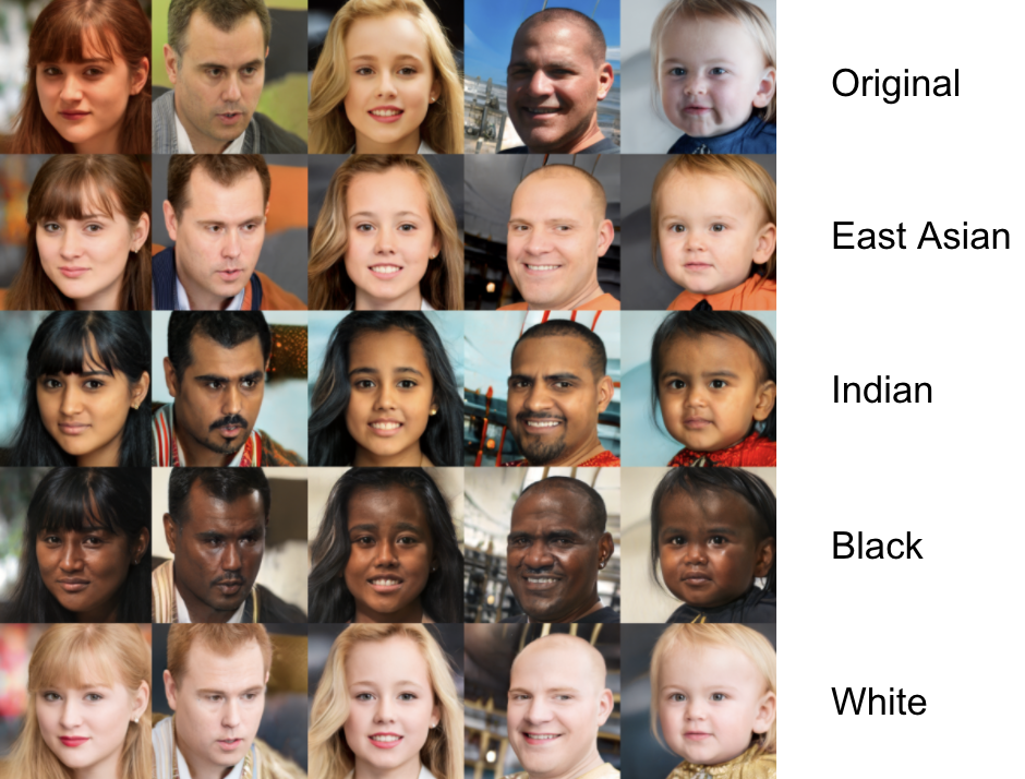
Figure 6: Examples of Synthetic datasets.

V-D Synthetic Datasets Generated Using StyleGAN2

Due to the insufficiency of samples after splitting by several protected attributes, existing datasets may not be sufficient. Inspired by [4], we propose a new synthetic dataset generated by StyleGAN2 [23] with a more complicated distribution, to facilitate experimental rather than observational analyses of the presented method.

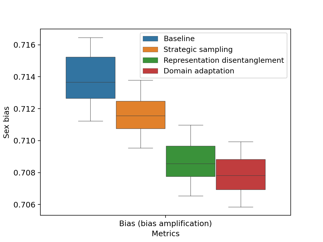
(a) Bias (bias amplification [45]).

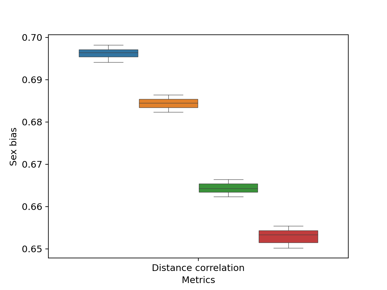
(b) Distance correlation [34].

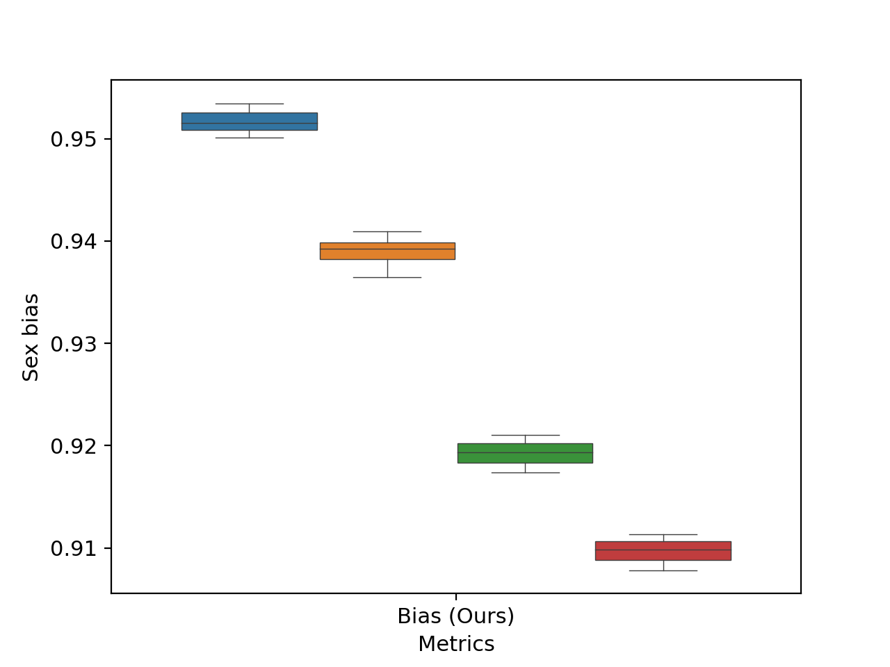
(c) RLB (MI baseline).

(d) RLB (adding mapping network).

Figure 7: Debiasing performance comparison of debiasing models on CelebA Dataset using box plots.

TABLE III: Debiasing performance comparison of debiasing models on CelebA Dataset.

	mAP			Bias (BA [45])	${dcor}^{2}$ [34]	MI / RLB (Ours)
	Female	Male	Overall	Sex	Sex	Sex
Baseline	75.8	72.2	74.3	0.714	0.697	0.636 / 0.954
Strategic sampling [28]	75.4	72.3	74.1	0.712	0.672	0.628 / 0.942
Representation disentanglement [12, 2, 19]	73.1	70.2	71.9	0.708	0.659	0.620 / 0.929
Domain adaptation [38, 15]	74.7	72.5	73.8	0.707	0.643	0.612 / 0.918
Domain independent training [40]	76.5	76.1	76.3	0.702	0.578	0.553 / 0.829

TABLE IV: Debiasing performance comparison of debiasing models on FairFace Dataset.

	Accuracy									Bias (BA [45])		${dcor}^{2}$ [34]		MI / RLB (Ours)
	Black		White		East Asian		Indian		Overall	Sex	Race	Sex	Race	Sex	Race
	F	M	F	M	F	M	F	M
Baseline	79.3	79.2	84.2	88.2	80.4	80.3	79.1	81.2	81.3	0.510	0.259	0.573	0.314	0.480 / 0.693	0.762 / 0.550
Strategic sampling [28]	80.5	80.3	83.7	86.4	79.5	79.6	79.2	81.1	80.7	0.508	0.257	0.552	0.309	0.468 / 0.675	0.757 / 0.546
Representation disentanglement [12, 2, 19]	78.6	78.5	82.5	84.5	78.5	78.6	78.1	79.3	78.6	0.505	0.255	0.546	0.286	0.448 / 0.646	0.736 / 0.531
Domain adaptation [38, 15]	80.7	80.6	83.9	85.6	79.7	79.8	79.9	80.1	79.8	0.504	0.255	0.531	0.281	0.437 / 0.631	0.729 / 0.526
Domain independent training [40]	82.5	82.4	85.3	87.1	82.5	82.5	82.3	82.5	83.5	0.501	0.253	0.478	0.247	0.361 / 0.521	0.658 / 0.475

Experiment Setup. We simulate the degree of bias by assigning the entropy of protected attributes, such as sex entropy $H^{s}_{i}=-[P(z^{f})logP(z^{f})+P(z^{m})logP(z^{m})]$ where $P(z^{f})$ is the percentage of female in the whole dataset. Next, given a source $\mathcal{S}_{0}$ from which the generated images are distinctive and high-quality, and a source $\mathcal{S}_{1}$ with four manually selected latent vectors as representatives for races, inside StyleGAN2 [23] pretrained on FFHQ [22], the mapping network $f$ produces $e_{0}^{(i)}$ and $e_{1}^{(j)}$ from $u_{0}^{(i)}\in\mathcal{S}_{0}$ and $u_{1}^{(j)}\in\mathcal{S}_{1}$, and the synthesis network $p$ generates an image $I_{ij}$ by taking $e_{0}^{(i)}$ at coarse spatial resolution $(4^{2}-8^{2})$ to bring high-level appearances (hair style, face shape) from $\mathcal{S}_{0}$, and $e_{1}^{(j)}$ at fine spatial resolution $(16^{2}-1024^{2})$ to obtain racial appearances (colors of eyes, hair, skin) from $\mathcal{S}_{1}$. Further, we generate a specific dataset according to the preset entropy. Finally, we train a ResNet-50 [17] on generated datasets with different sex entropy $H^{g}_{i}$ or race entropy $H^{r}_{i}$ to construct learned representation space $\mathcal{R}$ for evaluating our representation-level independent bias assessment on the balanced testing set with $H^{g}_{i}=0.693$ and $H^{r}_{i}=1.386$ at the balance point. We use skin color as a proxy to race in this experiment, same as Pilot Parliaments Benchmark (PPB) [6]. The end-to-end three-stage pipeline is shown in Fig. 5.

Results. As shown in Fig. 6, benefiting from mapping network to reduce feature entanglement, the generated images in different races maintain the similar appearance with different skin tone, which mitigates interference of appearance. A few observations can be drawn from the Fig. 4(b). First, RLB declines as the entropy increases. According to the definition of entropy, larger entropy implies a more balanced dataset, and therefore, RLB is consistent with degree of imbalance. Second, compared to sex entropy, race entropy has a stronger influence on RLB.

V-E Comparison With Debiased Models

Inspired by [40], we compare bias assessment metrics on four mainstream families of debiasing methods — (1) strategic sampling, (2) representation disentanglement, (3) domain adaptation and (4) domain independent training, with BA [45] and ${dcor}^{2}$ [34]. The ResNet-50 [17] pre-trained on ImageNet [8] (as baseline model) is used to predict attributes. We assess RLB of sex on CelebA dataset and both sex and race on FairFace dataset. Mean average precision (mAP) across cohorts is also presented as metric comparison for this multi-label classification.

Results. In order to illustrate the ability to capture model bias, the degree of imbalance of testing dataset is kept same, i.e. sex entropy of CelebA dataset is $0.667$, sex entropy and race entropy of FairFace dataset is $0.693$ and $1.386$. Besides, mutual information estimation (MI) corresponding with RLB is separably presented as ablation study of bias assessment with and without entropy. In Table III and Table IV, debiasing models are compared across rows and metrics are compared across columns. The results show that domain-independent training [40] performs the best with the most balanced mAP across all cohorts. In order to present variation and mean of different metrics in a more straightforward way, we conduct experiments with 50 different random seeds and calculate statistics of different metrics for sex bias in CelebA dataset [29] using box plot, as shown in Fig. 7. Comparing Fig. 7(a) with Fig. 7(d), we find that the confused four groups under BA [45] are clearly distinguished under RLB due to a larger range which can be used to stratify different degree of bias from more models without aliasing. Furthermore, comparing with ${dcor}^{2}$ in Fig. 7(b), RLB assesses sex bias with small variation. Also, comparing Fig. 7(c) and Fig. 7(d), RLB (adding mapping network) yields smaller variation and more robustness than MI baseline. Theoretically, different metrics for demographic bias construct a metric space rather than a normed space since there is no definition of zero point. Furthermore, in the absence of standard unit of bias and proper conversion between different metrics, we need to consider the absolute value instead of the relative value and the advantages (clear discrepancy and small variation) of RLB demonstrate a better precision.

VI Conclusion

We present a bias assessment metric to assess demographic bias in face recognition at the representation level and empirically demonstrate that RLB reflects the bias issues induced from imbalanced datasets and biased models. Our results show that the conclusions of previous work that use mAP across cohorts, BA and ${dcor}^{2}$ show large variation and may produce contradictory bias assessment scores when comparing more debiasing models since these metrics have not yielded clear discrepancy. Furthermore, the conclusions of prior work that use logits loss to evaluate debiasing performance may be inaccurate since spurious correlations may lead to inaccurate logits-level metrics. On the other hand, our independent representation-level bias can be not only used to evaluate the overall performance for bias mitigation, but also used to detect bias inside debiased models, which allows a more flexible and wider-range usage for studying bias in classification models.

References

- [1] E. Adeli, Q. Zhao, A. Pfefferbaum, E. V. Sullivan, L. Fei-Fei, J. C. Niebles, and K. M. Pohl. Representation learning with statistical independence to mitigate bias. In Proc. of the IEEE/CVF Winter Conf. on Applications of Computer Vision, pages 2513–2523, 2021.
- [2] M. Alvi, A. Zisserman, and C. Nellåker. Turning a blind eye: Explicit removal of biases and variation from deep neural network embeddings. In Proc. of the European Conf. on Computer Vision (ECCV) Workshops, pages 0–0, 2018.
- [3] A. Amini, A. P. Soleimany, W. Schwarting, S. N. Bhatia, and D. Rus. Uncovering and mitigating algorithmic bias through learned latent structure. In Proc. of the 2019 AAAI/ACM Conf. on AI, Ethics, and Society, pages 289–295, 2019.
- [4] G. Balakrishnan, Y. Xiong, W. Xia, and P. Perona. Towards causal benchmarking of bias in face analysis algorithms. In European Conf. on Computer Vision, pages 547–563. Springer, 2020.
- [5] M. I. Belghazi, A. Baratin, S. Rajeshwar, S. Ozair, Y. Bengio, A. Courville, and D. Hjelm. Mutual information neural estimation. In ICML, pages 531–540. PMLR, 2018.
- [6] J. Buolamwini and T. Gebru. Gender shades: Intersectional accuracy disparities in commercial gender classification. In S. A. Friedler and C. Wilson, editors, Proc. of the 1st Conf. on Fairness, Accountability and Transparency, volume 81 of Proc. of Machine Learning Research, pages 77–91. PMLR, 23–24 Feb 2018.
- [7] C. M. Cook, J. J. Howard, Y. B. Sirotin, J. L. Tipton, and A. R. Vemury. Demographic effects in facial recognition and their dependence on image acquisition: An evaluation of eleven commercial systems. IEEE Trans. on Biometrics, Behavior, and Identity Science, 1(1):32–41, 2019.
- [8] J. Deng, W. Dong, R. Socher, L. Li, Kai Li, and Li Fei-Fei. Imagenet: A large-scale hierarchical image database. In 2009 IEEE Conf. on Computer Vision and Pattern Recognition, pages 248–255, 2009.
- [9] M. D. Donsker and S. S. Varadhan. Asymptotic evaluation of certain markov process expectations for large time, i. Communications on Pure and Applied Mathematics, 28(1):1–47, 1975.
- [10] C. Dwork, M. Hardt, T. Pitassi, O. Reingold, and R. Zemel. Fairness through awareness. In Proc. of the 3rd innovations in theoretical computer science conf., pages 214–226, 2012.
- [11] C. Garvie and J. Frankle. Facial-recognition software might have a racial bias problem. The Atlantic, 7, 2016.
- [12] S. Gong, X. Liu, and A. K. Jain. Jointly de-biasing face recognition and demographic attribute estimation. In European Conf. on Computer Vision, pages 330–347. Springer, 2020.
- [13] S. Gong, X. Liu, and A. K. Jain. Mitigating face recognition bias via group adaptive classifier. In Proc. of the IEEE/CVF Conf. on Computer Vision and Pattern Recognition, pages 3414–3424, 2021.
- [14] P. Grother, M. Ngan, and K. Hanaoka. Face Recognition Vendor Test (FVRT): Part 3, Demographic Effects. National Institute of Standards and Technology, 2019.
- [15] J. Guo, X. Zhu, C. Zhao, D. Cao, Z. Lei, and S. Z. Li. Learning meta face recognition in unseen domains. In CVPR, pages 6163–6172, 2020.
- [16] M. Hardt, E. Price, and N. Srebro. Equality of opportunity in supervised learning. In Proc. of the 30th International Conf. on Neural Information Processing Systems, NIPS’16, page 3323–3331, Red Hook, NY, USA, 2016. Curran Associates Inc.
- [17] K. He, X. Zhang, S. Ren, and J. Sun. Deep residual learning for image recognition. In Proc. of the IEEE conf. on computer vision and pattern recognition, pages 770–778, 2016.
- [18] N. O. Hodas and P. Stinis. Doing the impossible: Why neural networks can be trained at all. Frontiers in psychology, 9:1185, 2018.
- [19] A. Jaiswal, D. Moyer, G. Ver Steeg, W. AbdAlmageed, and P. Natarajan. Invariant representations through adversarial forgetting. In Proc. of the AAAI Conf. on Artificial Intelligence, volume 34, pages 4272–4279, 2020.
- [20] A. Jaiswal, R. Y. Wu, W. Abd-Almageed, and P. Natarajan. Unsupervised Adversarial Invariance. In S. Bengio, H. Wallach, H. Larochelle, K. Grauman, N. Cesa-Bianchi, and R. Garnett, editors, Advances in Neural Information Processing Systems 31, pages 5097–5107. Curran Associates, Inc., 2018.
- [21] K. Karkkainen and J. Joo. Fairface: Face attribute dataset for balanced race, gender, and age for bias measurement and mitigation. In Proc. of the IEEE/CVF Winter Conf. on Applications of Computer Vision, pages 1548–1558, 2021.
- [22] T. Karras, S. Laine, and T. Aila. A style-based generator architecture for generative adversarial networks. In Proc. of the IEEE/CVF Conf. on Computer Vision and Pattern Recognition, pages 4401–4410, 2019.
- [23] T. Karras, S. Laine, M. Aittala, J. Hellsten, J. Lehtinen, and T. Aila. Analyzing and improving the image quality of stylegan. In Proc. of the IEEE/CVF Conf. on Computer Vision and Pattern Recognition, pages 8110–8119, 2020.
- [24] B. Kim, H. Kim, K. Kim, S. Kim, and J. Kim. Learning not to learn: Training deep neural networks with biased data. In Proc. of the IEEE/CVF Conf. on Computer Vision and Pattern Recognition, pages 9012–9020, 2019.
- [25] Y. LeCun, L. Bottou, Y. Bengio, and P. Haffner. Gradient-based learning applied to document recognition. Proc. of the IEEE, 86(11):2278–2324, 1998.
- [26] Y. LeCun, C. Cortes, and C. Burges. Mnist handwritten digit database, 2010.
- [27] Y. Li, Y. Li, and N. Vasconcelos. Resound: Towards action recognition without representation bias. In Proc. of the European Conf. on Computer Vision (ECCV), pages 513–528, 2018.
- [28] Y. Li and N. Vasconcelos. Repair: Removing representation bias by dataset resampling. In Proc. of the IEEE/CVF Conf. on Computer Vision and Pattern Recognition, pages 9572–9581, 2019.
- [29] Z. Liu, P. Luo, X. Wang, and X. Tang. Deep learning face attributes in the wild. In Proc. of the IEEE International Conf. on computer vision, pages 3730–3738, 2015.
- [30] B. Maze, J. Adams, J. A. Duncan, N. Kalka, T. Miller, C. Otto, A. K. Jain, W. T. Niggel, J. Anderson, J. Cheney, et al. Iarpa janus benchmark-c: Face dataset and protocol. In 2018 International Conf. on Biometrics (ICB), pages 158–165. IEEE, 2018.
- [31] K. Pezdek, I. Blandón-Gitlin, and C. Moore. Children’s face recognition memory: more evidence for the cross-race effect. The J. of applied psychology, 88 4:760–3, 2003.
- [32] R. Ragonesi, R. Volpi, J. Cavazza, and V. Murino. Learning unbiased representations via mutual information backpropagation. In Proc. of the IEEE/CVF Conf. on Computer Vision and Pattern Recognition, pages 2729–2738, 2021.
- [33] A. Romanov, M. De-Arteaga, H. Wallach, J. Chayes, C. Borgs, A. Chouldechova, S. Geyik, K. Kenthapadi, A. Rumshisky, and A. T. Kalai. What’s in a name? reducing bias in bios without access to protected attributes. arXiv preprint arXiv:1904.05233, 2019.
- [34] G. J. Székely, M. L. Rizzo, N. K. Bakirov, et al. Measuring and testing dependence by correlation of distances. The annals of statistics, 35(6):2769–2794, 2007.
- [35] A. Torralba and A. A. Efros. Unbiased look at dataset bias. In CVPR 2011, pages 1521–1528. IEEE, 2011.
- [36] K. Vangara, M. C. King, V. Albiero, K. Bowyer, et al. Characterizing the variability in face recognition accuracy relative to race. In Proc. of the IEEE/CVF Conf. on Computer Vision and Pattern Recognition Workshops, pages 0–0, 2019.
- [37] M. Wang and W. Deng. Deep face recognition: A survey. Neurocomputing, 429:215–244, 2021.
- [38] M. Wang, W. Deng, J. Hu, X. Tao, and Y. Huang. Racial faces in the wild: Reducing racial bias by information maximization adaptation network. In Proc. of the IEEE/CVF International Conf. on Computer Vision, pages 692–702, 2019.
- [39] T. Wang, J. Zhao, M. Yatskar, K.-W. Chang, and V. Ordonez. Balanced datasets are not enough: Estimating and mitigating gender bias in deep image representations. In Proc. of the IEEE/CVF International Conf. on Computer Vision, pages 5310–5319, 2019.
- [40] Z. Wang, K. Qinami, I. C. Karakozis, K. Genova, P. Nair, K. Hata, and O. Russakovsky. Towards fairness in visual recognition: Effective strategies for bias mitigation. In Proc. of the IEEE/CVF Conf. on Computer Vision and Pattern Recognition, pages 8919–8928, 2020.
- [41] Q. Xie, Z. Dai, Y. Du, E. Hovy, and G. Neubig. Controllable invariance through adversarial feature learning. In I. Guyon, U. V. Luxburg, S. Bengio, H. Wallach, R. Fergus, S. Vishwanathan, and R. Garnett, editors, Advances in Neural Information Processing Systems, volume 30. Curran Associates, Inc., 2017.
- [42] Ya Wang, Tianlong Bao, Chunhui Ding, and Ming Zhu. Face recognition in real-world surveillance videos with deep learning method. In 2017 2nd International Conf. on Image, Vision and Computing (ICIVC), pages 239–243, 2017.
- [43] B. H. Zhang, B. Lemoine, and M. Mitchell. Mitigating unwanted biases with adversarial learning. In Proc. of the 2018 AAAI/ACM Conf. on AI, Ethics, and Society, pages 335–340, 2018.
- [44] Z. Zhang, Y. Song, and H. Qi. Age progression/regression by conditional adversarial autoencoder. In Proc. of the IEEE Conf. on computer vision and pattern recognition, pages 5810–5818, 2017.
- [45] J. Zhao, T. Wang, M. Yatskar, V. Ordonez, and K.-W. Chang. Men also like shopping: Reducing gender bias amplification using corpus-level constraints. In Proc. of the 2017 Conf. on Empirical Methods in Natural Language Processing, pages 2941–2951, 2017.
- [46] X. Zhu, D. Anguelov, and D. Ramanan. Capturing long-tail distributions of object subcategories. In 2014 IEEE Conf. on Computer Vision and Pattern Recognition, pages 915–922, 2014.