Orientability of space from electromagnetic quantum fluctuations

Abstract

Whether the $3-$space where we live is a globally orientable manifold $M_{3}$, and whether the local laws of physics require that $M_{3}$ be equipped with a canonical orientation, are among the important unsettled questions in cosmology and quantum field theory. It is often assumed that a test for spatial orientability requires a global journey across the whole $3-$space to check for orientation-reversing closed paths. Since such a global expedition is not feasible, physically motivated theoretical arguments are usually offered to support the choice of canonical time orientation for the $4-$dimensional spacetime manifold, and space orientation for $3-$space. One can certainly take advantage of such theoretical arguments to support these assumptions on orientability, but the ultimate answer should rely on cosmological observations or local experiments, or can come from a topological fundamental theory of physics. In a recent paper we have argued that it is potentially possible to locally access the the $3-$space orientability of Minkowski empty spacetime through physical effects involving point-like ’charged’ objects under vacuum quantum electromagnetic fluctuations. More specifically, we have studied the stochastic motions of a charged particle and an electric dipole subjected to these fluctuations in Minkowski spacetime, with either an orientable or a non-orientable $3-$space topology, and derived analytical expressions for a statistical orientability indicator in these two flat topologically inequivalent manifolds. For the charged particle, we have shown that it is possible to distinguish the two topologies by contrasting the evolution of their respective indicators. For the point electric dipole we have found that a characteristic inversion pattern exhibited by the curves of the orientability indicator is a signature of non-orientability, making it possible to locally probe the orientability of Minkowski $3-$space in itself. Here, to shed some additional light on the spatial orientability, we briefly review these results, and also discuss some of its features and consequences. The results might be seen as opening the way to a conceivable experiment involving quantum vacuum electromagnetic fluctuations to look into the spatial orientability of Minkowski empty spacetime.

1 Introduction

In the framework of general relativity the Universe is described as a four-dimensional differentiable manifold locally endowed with a spatially homogeneous and isotropic Friedmann–Lemaître–Robertson–Walker (FLRW) metric. Geometry is a local attribute that brings about intrinsic curvature, whereas topology is a global feature of a manifold related, for example, to compactness and orientability. The FLRW spatial geometry constrains but does not specify the topology of the spatial sections, $M_{3}$, of the space-time manifold, which we assume to be of the form $\mathcal{M}_{4}=\mathbb{R}\times M_{3}$. In the FLRW description of the Universe, two diverse sets of fundamental questions are related to, first, the $3-$geometry; second, to the topology of spatial sections $M_{3}$. Regarding the latter, at the cosmological level it is expected that one should be able to detect the spatial topology through cosmic microwave background radiation (CMB) or (and) stochastic primordial gravitational waves [1, 2]. However, so far, direct searches for a nontrivial topology of $M_{3}$, using CMB data from Wilkinson Microwave Anisotropy Probe (WMAP) and Planck collaborations, have found no convincing evidence of nontrivial topology below the radius of the last scattering surface [3, 4, 5, 6, 7, 8, 9]. This absence of evidences does not exclude the possibility of a FLRW  universe with a detectable nontrivial spatial topology [10, 11, 12].

It is well-known that the topological properties of a manifold antecede its geometrical features and the differential tensor structure with which the physical theories are formulated. Thus, it is relevant to determine whether, how and to what extent physical results depend upon or are somehow affected by a nontrivial topology. Since the net role played by the spatial topology is more properly examined in static space-times, the dynamical degrees of freedom of which are frozen, here we focus on the static Minkowski space-time, whose spatial geometry is Euclidean. However, rather than the general topology of the spatial sections $M_{3}$ of Minkowski space-time, in this work we investigate its topological property called orientability, which is related to the existence of orientation-reversing closed paths on the spatial section $M_{3}$. Questions as to whether the $3-$space of Minkowski space-time, which is the standard arena of quantum field theory, is necessarily an orientable manifold, or to what extent the known laws of physics require a canonical spatial orientation are among the underlying primary concerns of this work.

To be more precise regarding the setting of the present work, let us first briefly provide some mathematical results. The spatial section $M_{3}$ of the Minkowski spacetime manifold $\mathcal{M}_{4}=\mathbb{R}\times M_{3}$ is usually taken to be the simply-connected Euclidean space $\mathbb{E}^{3}$, but it is known mathematical result that it can also be any one of the possible $17$ topologically distinct quotient manifolds $M_{3}=\mathbb{E}^{3}/\Gamma$, where $\Gamma$ is a discrete group of isometries or holonomies acting freely on the covering space $\mathbb{E}^{3}$. The action of $\Gamma$ tiles the covering manifold $\mathbb{E}^{3}$ into identical cells which are copies of what is known as fundamental domain (FD) fundamental cell or polyhedron (FC or FP). So, the multiple-connectedness gives rise to periodic conditions (repeated cells) in the simply-connected covering manifold $\mathbb{E}^{3}$ that are defined by the action of the group $\Gamma$ on $\mathbb{E}^{3}$. Different groups $\Gamma$ give rise to different periodicities on the covering manifold $\mathbb{E}^{3}$, which in turn define different Euclidean spatial topologies $M_{3}$ for Minkowski spacetime. These mathematical results make it explicit that besides the simply-connected $\mathbb{E}^{3}$ there is a variety of topological possibilities ($17$ classes) for the spatial section of Minkowski spacetime. The potential consequences of multiple-connectedness for physics come about when, for example, one takes into account that in a manifold with periodic boundary conditions only certain modes of fields can exist. In this way, a nontrivial topology may leave its signature on the expectation values of local physical quantities[19]. So, for example, the energy density for a scalar field in Minkowski space-time with nontrivial spatial section is shifted from the corresponding result for the Minkowski space-time with trivial spatial topology. This is the Casimir effect of topological origin [20, 21, 22, 23, 24, 25].

Regarding orientability, the central issue of this work, three important points should be emphasized. First, we mention that it is widely assumed, implicitly or explicitly, that a four-dimensional manifold $\mathcal{M}_{4}=\mathbb{R}\times M_{3}$ that models the physical world is spacetime orientable and, additionally, that it is separately time and space orientable. Second, eight out of the above-mentioned $17$ quotient flat $3-$manifolds are non-orientable [13, 14, 15, 16, 17, 18]. A non-orientable $3-$space is then a concrete mathematical possibility among the quotient manifolds $M_{3}=\mathbb{E}^{3}/\Gamma$, and it comes about when the holonomy group $\Gamma$ contains at least a flip or reflexion as one of its elements. Finally, it is generally assumed that, being a global property, the $3-$space orientability cannot be tested locally. In this way, to disclose the spatial orientability of our physical world one would have to make trips along some specific closed paths around $3-$space to check, for example, whether one returns with left- and right-hand sides exchanged.

Since such a global journey across the whole $3-$space is not feasible one might think that spatial orientability cannot be probed. In this way, one would have either to answer the orientability question through cosmological observations or local experiments. Hence, assuming that spatial orientability is a falsifiable property of $3-$space, a question that arises is whether spatial orientability can be subjected to local tests. Our main goal in this work is to present a way to tackle this question. To this end, we have investigated[26] stochastic motions of a charge particle and an electric dipole under vacuum quantum fluctuations of the electromagnetic field in Minkowski spacetime with two inequivalent spatial topologies, namely the non-orientable slab with flip and the orientable slab, which are often denoted by the symbols $E_{17}$ and $E_{16}$, respectively [17, 18]. Manifolds endowed with these topologies turned out to be appropriate to identify orientability or non-orientability signatures through the stochastic motions of point-like particles in Minkowski spacetime. In the next section, to shed some additional light on spatial orientability, we briefly review the most significant results of our article, Ref. Lemos-Reboucas2021, and discuss some of their consequences.

2 Main results and their interpretation

The general idea underlying our work is to perform a comparative study of the time evolution of physical systems in Minkowski spacetime with orientable and non-orientable spatial sections. To this end, the physical systems chosen are a point charged particle and a point electric dipole under vacuum quantum electromagnetic fluctuations. We shall describe the results for the dipole only because they are more significant — see Ref. Lemos-Reboucas2021 for the point charge case.

2.1 The setting and the physical system

We begin by recalling that simply-connected spacetime manifolds are necessarily orientable. On the other hand, the product of two manifolds is simply-connected if and only if the factors are. Thus, the space-orientability of Minkowski spacetime manifold $\mathcal{M}_{4}=\mathbb{R}\times M_{3}$ reduces to orientability of the $3-$space $M_{3}$. In this paper, we shall consider the topologically nontrivial spaces $E_{16}$ and $E_{17}$. The slab space $E_{16}$ is constructed by tessellating $\mathbb{E}^{3}$ by equidistant parallel planes, so it has only one compact dimension associated with a direction perpendicular to those planes. Taking the $x$-direction as compact, one has that, with $n_{x}\in\mathbb{Z}$ and $a>0$, points $(x,y,z)$ and $(x+n_{x}a,y,z)$ are identified in the case of the slab space $E_{16}$. The slab space with flip $E_{17}$ involves an additional inversion of a direction orthogonal to the compact direction, that is, one direction in the tessellating planes is flipped as one moves from one plane to the next. Letting the flip be in the $y$-direction, the identification of points $(x,y,z)$ and $(x+n_{x}a,(-1)^{n_{x}}y,z)$ defines the $E_{17}$ topology. The slab space $E_{16}$ is orientable whereas the slab space with flip $E_{17}$ is non-orientable.

The physical system we consider consists of a point electric dipole with moment $\bf p$ and mass $m$ that is locally subject to vacuum fluctuations of the electric field ${\bf E}({\bf x},t)$ in Minkowski spacetime $\mathcal{M}_{4}$ with the metric $\eta_{\mu\nu}=\mbox{diag}(+1,-1,-1,-1)$. The topology of the spatial section $M_{3}$ is taken to be either $E_{16}$ (orientable) or $E_{17}$ (non-orientable) instead of $\mathbb{E}^{3}$.

The nonrelativistic motion of the dipole is locally determined by

$$m\frac{d{\bf v}}{dt}={\bf p}\cdot{\mbox{\boldmath$\nabla$}}{\bf E}({\bf x},t)\,,$$ (1)

where $\mathbf{v}$ is the dipole’s velocity and $\mathbf{x}$ its position at time $t$. We assume that the dipole practically does not move on the time scales of interest. Thus the dipole has a negligible displacement, and we can ignore the time dependence of $\mathbf{x}$. So, $\mathbf{x}$ is taken to be constant in what follows [27, 28].

Assuming the dipole is initially at rest, integration of Eq. (1) yields

$${\bf v}({\bf x},t)=\frac{1}{m}p_{j}\int_{0}^{t}\partial_{j}{\bf E}({\bf x},t^{\prime})\,dt^{\prime}$$ (2)

with $\partial_{j}=\partial/\partial x_{j}$ and summation over repeated indices implied.

The mean squared speed in each of the three independent directions $i=x,y,z$ is given by

$$\Bigl{\langle}\Delta v^{2}_{i}\Bigr{\rangle}=\frac{p_{j}p_{k}}{m^{2}}\int_{0}^{t}\int_{0}^{t}\Bigl{\langle}\bigl{(}\partial_{j}E_{i}({\bf x},t^{\prime})\bigr{)}\bigl{(}\partial_{k}E_{i}({\bf x},t^{\prime\prime})\bigr{)}\Bigr{\rangle}\,dt^{\prime}dt^{\prime\prime}\,,$$ (3)

which can be conveniently rewritten as

$$\Bigl{\langle}\Delta v^{2}_{i}\Bigr{\rangle}=\lim_{{\bf x}^{\prime}\to{\bf x}}\frac{p_{j}p_{k}}{m^{2}}\int_{0}^{t}\int_{0}^{t}\partial_{j}\partial_{k}^{\,\prime}\Bigl{\langle}E_{i}({\bf x},t^{\prime})E_{i}({\bf x}^{\prime},t^{\prime\prime})\Bigr{\rangle}\,dt^{\prime}dt^{\prime\prime}$$ (4)

where $\partial_{k}^{\,\prime}=\partial/\partial x_{k}^{\prime}$ and there is no summation over $i$. Following Ref. yf04, we assume that the electric field is a sum of quantum $\mathbf{E}_{q}$ and classical $\mathbf{E}_{c}$ parts. Since ${\bf E}_{c}$ is not subject to quantum fluctuations and $\langle{\bf E}_{q}\rangle=0$, the two-point function $\langle E_{i}({\bf x},t)E_{i}({\bf x}^{\prime},t^{\prime})\rangle$ in equation (4) involves only the quantum part $\mathbf{E}_{q}$ of the electric field.

In Minkowski spacetime with a topologically nontrivial spatial section, the spatial separation $r^{2}$ that enters the electric field correlation functions takes a form that captures the periodic boundary conditions imposed on the covering space $\mathbb{E}^{3}$ by the covering group $\Gamma$, which characterize the spatial topology. In consonance with Ref. st06, the spatial separations for $E_{16}$ and $E_{17}$ are

$$E_{16}:\qquad r^{2} = (x-x^{\prime}-n_{x}a)^{2}+(y-y^{\prime})^{2}+(z-z^{\prime})^{2},$$ (5)

$$E_{17}:\qquad r^{2} = (x-x^{\prime}-n_{x}a)^{2}+(y-(-1)^{n_{x}}y^{\prime})^{2}+(z-z^{\prime})^{2}.$$ (6)

2.2 Orientability indicator

The orientability indicator that we will consider is defined by replacing the electric field correlation functions in Eq. (4) by their renormalized counterparts[26]. For a dipole oriented along the $y$-axis the dipole moment is ${\bf p}=(0,p,0)$ and we have

$$^{{}^{(y)}}{\!}\mbox{\large$I$}_{v^{2}_{i}}^{E_{17}}({\bf x},t)=\lim_{{\bf x}^{\prime}\to{\bf x}}\frac{p^{2}}{m^{2}}\int_{0}^{t}\int_{0}^{t}\partial_{y}\partial_{y^{\prime}}\Bigl{\langle}E_{i}({\bf x},t^{\prime})E_{i}({\bf x}^{\prime},t^{\prime\prime})\Bigr{\rangle}_{ren}^{E_{17}}\,dt^{\prime}dt^{\prime\prime}\,,$$ (7)

where the left superscript within parentheses indicates the dipole’s orientation.

The renormalized correlation functions are given by[26]

$$\bigl{\langle}E_{i}({\bf x},t)E_{i}({\bf x}^{\prime},t^{\prime})\bigr{\rangle}_{ren}=\frac{\partial}{\partial x_{i}}\frac{\partial}{\partial{x^{\prime}}_{i}}D_{ren}({\bf x},t;{\bf x}^{\prime},t^{\prime})-\frac{\partial}{\partial t}\frac{\partial}{\partial t^{\prime}}D_{ren}({\bf x},t;{\bf x^{\prime}},t^{\prime})$$ (8)

where

$$D_{ren}({\bf x},t;{\bf x}^{\prime},t^{\prime})=\sum\limits_{{n_{x}=-\infty}}^{{\infty\;\;\prime}}\frac{1}{4\pi^{2}(\Delta t^{2}-r^{2})}$$ (9)

and where $\Delta t=t-t^{\prime}$, $\,\sum^{\;{}^{\prime}}$ indicates that the Minkowski contribution term $n_{x}=0$ is excluded from the summation, and the spatial separation for $E_{17}$ is given by Eq. (6).

The Hadamard function $D({\bf x},t;{\bf x}^{\prime},t^{\prime})$ for the multiply-connected space is defined by including the term with $n_{x}=0$ in the summation (9). Thus, $D_{ren}=D-D_{0}$, where $D_{0}$ is the Hadamard function for the simply-connected space.

Before calculating the components of the orientability indicator in equation (7), we point out that from equations (4) and (7) – (9) one can figure out a general definition of the orientability indicator as

$$\mbox{\large$I$}_{v^{2}_{i}}^{MC}=\Bigl{\langle}\Delta v_{i}^{2}\Bigr{\rangle}^{MC}-\;\,\Bigl{\langle}\Delta v_{i}^{2}\Bigr{\rangle}^{SC},$$ (10)

where $\bigl{\langle}\Delta v_{i}^{2}\bigr{\rangle}$ is the mean square velocity dispersion, and the superscripts $SC$ and $MC$ stand for simply- and multiply-connected manifold, respectively. The right-hand side of (10) is defined by first taking the difference of the two terms with ${\bf x}^{\prime}\neq{\bf x}$ and then setting ${\bf x}^{\prime}={\bf x}$ (coincidence limit).

The components of the orientability indicator for the dipole in $E_{17}$ are [26]

$$^{{}^{(y)}}{\!}\mbox{\large$I$}_{v^{2}_{x}}^{E_{17}}({\bf x},t)=-\frac{4p^{2}}{\pi^{2}m^{2}}\sum\limits_{{n_{x}=-\infty}}^{{\infty\;\;\prime}}(-1)^{n_{x}}\bigg{\{}2I_{1}+3(r^{2}-r_{x}^{2}+6r_{y}^{2})I_{2}+24(r^{2}-r_{x}^{2})r_{y}^{2}I_{3}\bigg{\}},$$ (11)

$${}^{{}^{(y)}}{\!}\mbox{\large$I$}_{v^{2}_{y}}^{E_{17}}({\bf x},t) = -\frac{2p^{2}}{\pi^{2}m^{2}}\sum\limits_{{n_{x}=-\infty}}^{{\infty\;\;\prime}}(-1)^{n_{x}}\bigg{\{}(5-3(-1)^{n_{x}})I_{1}$$ (12)

$$+ 6[r^{2}+(7-6(-1)^{n_{x}})r_{y}^{2}]I_{2}+48[r^{2}-(-1)^{n_{x}}r_{y}^{2}]r_{y}^{2}I_{3}\bigg{\}}$$

and

$$^{{}^{(y)}}{\!}\mbox{\large$I$}_{v^{2}_{z}}^{E_{17}}({\bf x},t)=-\frac{4p^{2}}{\pi^{2}m^{2}}\sum\limits_{{n_{x}=-\infty}}^{{\infty\;\;\prime}}(-1)^{n_{x}}\bigg{\{}2I_{1}+3(r^{2}+6r_{y}^{2})I_{2}+24r^{2}r_{y}^{2}I_{3}\bigg{\}}.$$ (13)

where, with $\Delta t=t^{\prime}-t^{\prime\prime}$,

$$I_{1}=\int_{0}^{t}\int_{0}^{t}\frac{dt^{\prime}dt^{\prime\prime}}{(\Delta t^{2}-r^{2})^{3}}=\frac{t}{16}\bigg{[}\frac{4t}{r^{4}(t^{2}-r^{2})}+\frac{3}{r^{5}}\ln\frac{(r-t)^{2}}{(r+t)^{2}}\bigg{]},$$ (14)

$$I_{2}=\int_{0}^{t}\int_{0}^{t}\frac{dt^{\prime}dt^{\prime\prime}}{(\Delta t^{2}-r^{2})^{4}}=\frac{1}{6r}\frac{\partial I_{1}}{\partial r}=\frac{t}{96}\bigg{[}\frac{4t(9r^{2}-7t^{2})}{r^{6}(t^{2}-r^{2})^{2}}-\frac{15}{r^{7}}\ln\frac{(r-t)^{2}}{(r+t)^{2}}\bigg{]},$$ (15)

$$I_{3}=\int_{0}^{t}\int_{0}^{t}\frac{dt^{\prime}dt^{\prime\prime}}{(\Delta t^{2}-r^{2})^{5}}=\frac{1}{8r}\frac{\partial I_{2}}{\partial r}=\frac{t}{768}\bigg{[}\frac{4t(57t^{4}-136r^{2}t^{2}+87r^{4})}{r^{8}(t^{2}-r^{2})^{3}}+\frac{105}{r^{9}}\ln\frac{(r-t)^{2}}{(r+t)^{2}}\bigg{]}.$$ (16)

In Eqs. (11) to (16) one must put

$$r = \sqrt{n_{x}^{2}a^{2}+2(1-(-1)^{n_{x}})y^{2}},$$

$$r_{x}^{2} = n_{x}^{2}a^{2},\qquad r_{y}^{2}=2(1-(-1)^{n_{x}})y^{2}.$$ (17)

The components of the dipole orientability indicator for the slab space $E_{16}$ are obtained from those for $E_{17}$ by setting $r_{x}^{2}=r^{2},r_{y}=0$, and replacing $(-1)^{n_{x}}$ by $1$ everywhere. Therefore, we have

$${}^{{}^{(y)}}{\!}\mbox{\large$I$}_{v^{2}_{x}}^{E_{16}}({\bf x},t) = -\frac{8p^{2}}{\pi^{2}m^{2}}\sum\limits_{{n_{x}=-\infty}}^{{\infty\;\;\prime}}I_{1},$$ (18)

$${}^{{}^{(y)}}{\!}\mbox{\large$I$}_{v^{2}_{y}}^{E_{16}}({\bf x},t) = -\frac{4p^{2}}{\pi^{2}m^{2}}\sum\limits_{{n_{x}=-\infty}}^{{\infty\;\;\prime}}(I_{1}+3r^{2}I_{2}),$$ (19)

$${}^{{}^{(y)}}{\!}\mbox{\large$I$}_{v^{2}_{z}}^{E_{16}}({\bf x},t) = -\frac{4p^{2}}{\pi^{2}m^{2}}\sum\limits_{{n_{x}=-\infty}}^{{\infty\;\;\prime}}(2I_{1}+3r^{2}I_{2}),$$ (20)

in which $r=|n_{x}|a$.

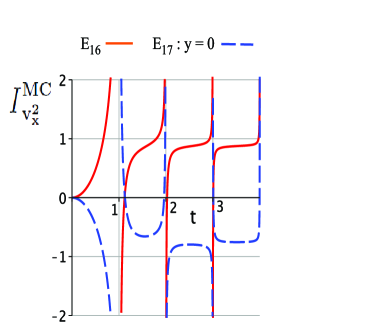
Figure 1: Time evolution of the orientability indicator (11), in units of $p^{2}/m^{2}$, for a point electric dipole with mass $m$ and dipole moment $p$, oriented in the flip $y-$direction, in Minkowski spacetime with non-orientable $E_{17}$ and orientable $E_{16}$ spatial topologies, with compact length $a=1$. The solid and dashed lines stand for the indicator curves for a dipole in $3-$space with $E_{16}$ and $E_{17}$ topologies, respectively. For the inhomogeneous topology $E_{17}$ the dipole is at $P_{0}=(x,0,z)$ to freeze out the topological inhomogeneity degree of freedom[26]. Both orientability indicator curves do present a periodicity pattern, but the curve for the non-orientable $E_{17}$ exhibits a different kind of periodicity characterized by a distinctive inversion pattern. Non-orientability is responsible for this pattern of sequential inversions, which is absent in the indicator curve for the orientable $E_{16}$.

2.3 Analysis of the results

Since equations (11)-(13) and (18)-(20) are too complicated to allow a straightforward interpretation, we plot figures for the components of the orientability indicator. Figures 1 and 2 arise from Eqs.  (11) – (13) as well as (18) – (20), with the topological length $a=1$ and $n_{x}\neq 0$ ranging from $-50$ to $50$. In Fig. 1 and Fig. 2 the solid lines stand for the curves of the orientability indicator for the dipole in Minkowski spacetime with $E_{16}$ orientable spatial topology, whereas the dashed lines correspond to the curves of the orientability indicator curves for the dipole located at $P_{0}=(x,0,z)$ in a $3-$space with $E_{17}$ non-orientable topology.

In the case of the $x$-component, the time evolution curves of the orientability indicator for $E_{16}$ and $E_{17}$, shown in Fig. 1, present a common periodicity but with distinguishable patterns. The orientability indicator curve for $E_{17}$ displays a distinctive sort of periodicity characterized by an inversion pattern. Non-orientability gives rise to this pattern of successive inversions, which does not occurs in the case of the orientable $E_{16}$.

The differences become more conspicuous when one considers the $y$-component of the orientability indicator, shown in Fig. 2. The non-orientability of $E_{17}$ is disclosed by an inversion pattern whose structure is more striking than the one for the $x$-component. The orientability indicator curves for $E_{17}$ form a pattern of alternating upward and downward “horns”, making the non-orientability of $E_{17}$ unmistakably identifiable. The $z$-component of the indicator behaves the same way [26].

The characteristic inversion pattern exhibited exhibited by the dipole indicator curves makes it possible to identify the non-orientability of the manifold $E_{17}$ in itself, with no need of a comparison with the indicator curves for its orientable counterpart $E_{16}$. However, this sort of comparison is necessary in the point charge case, as discussed in detail in Ref. Lemos-Reboucas2021.

In brief, it may be possible to unveil a putative non-orientability of the spatial section of Minkowski spacetime by local means, namely by the stochastic motions of charged point-like particles caused by electromagnetic quantum vacuum fluctuations. If the motion of a point electric dipole is taken as probe, non-orientability can be intrinsically detected by the inversion pattern of the dipole curves of the orientability indicator (10).

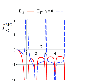
Figure 2: Time evolution of the orientability indicator (12) under the same conditions as those of Fig. 1. The orientability indicator curve for $E_{17}$ again exhibits a characteristic inversion pattern but now different from the one for the $v_{x}$-component shown in Fig. 1. For the $v_{y}$-component displayed here the non-orientability signature can be recognized in the pattern of consecutive upward and downward horn-like figures formed by the dashed curve.

3 Concluding remarks

In general relativity and quantum field theory spacetime is modeled as a differentiable manifold, which is a topological space endowed with a differential structure. It is generally assumed that the spacetime manifolds involved in these frameworks are entirely orientable, meaning that they are separately space and time orientable. The theoretical arguments used to adopt these assumptions on orientability combine the space-and-time universality of the basic local rules of physics with physically well-defined (thermodynamically) local arrow of time, CP violation and CPT invariance [42, 43, 44]. One can certainly use such reasonings in support of the standard assumptions on the global orientability structure of spacetimes. Nevertheless, it is legitimate to expect that the ultimate answer to questions regarding the orientability of spacetime manifolds should rely on astro-cosmological observations or local experiments, or even might come from a fundamental topological theory in physics.

In the physics at daily and even astrophysical length and time scales, we do not encounter signs or hints of non-orientability. This being true, the open question that remains is whether the physically well-defined local orientations can be extended to microscopic or cosmological scales.

At the cosmological scale, one would think at first sight that to disclose spatial orientability one would have to make a trip around the whole $3-$space to check for orientation-reversing paths. However, a determination of the spatial topology (detection and subsequent reconstruction of the topology) through the so-called circles in the sky [47], for example, would bring out as a bonus an answer to the $3-$space orientability problem at the cosmological scale. However, no convincing evidence of nontrivial spatial topology below the radius of the last scattering surface has been found up to now[3, 4, 5, 6, 7, 8, 9].

Parallel to these works, in this article we have addressed the question as to whether electromagnetic quantum vacuum fluctuations can be used to bring out the spatial orientability of Minkowski spacetime, in which the possible effects of the dynamical degree of freedom of FLRW spacetime is frozen in order to separate the topological and dynamical roles on the orientability problem. We have found that there exists a characteristic inversion pattern exhibited by the the curves of our orientability indicator (10) for a dipole in the case of $E_{17}$, signaling that the non-orientability of $E_{17}$ can be detected by per se, that is, with no need for comparisons. Thus, the inversion pattern of the orientability indicator curves for the dipole is a signature of the reflection holonomy, which is expected to be present in the orientability indicator curves for the dipole in all remaining seven non-orientable topologies that contain a flip holonomy, namely the four Klein spaces ($E_{7}$ to $E_{10}$) and the chimney-with-flip class ($E_{13}$ to $E_{15}$).

Observation of physical phenomena and controlled experiments are essential to our understanding of nature. Our results indicate the possibility of a local experiment to unveil spatial non-orientability through stochastic motions of point-like particles under electromagnetic quantum vacuum fluctuations. The present paper may be seen as a hint of a possible way to locally probe the spatial orientability of Minkowski spacetime.

References

- [1] G.F.R. Ellis, Gen. Rel. Grav. 2, 7 (1971); M. Lachièze-Rey and J.P. Luminet, Phys. Rep. 254, 135 (1995); G.D. Starkman, Class. Quantum Grav. 15, 2529 (1998); J. Levin, Phys. Rep. 365, 251 (2002); M.J. Rebouças and G.I. Gomero, Braz. J. Phys. 34, 1358 (2004); M.J. Rebouças, A Brief Introduction to Cosmic Topology, in Proc. XIth Brazilian School of Cosmology and Gravitation, eds. M. Novello and S.E. Perez Bergliaffa (Americal Institute of Physics, Melville, NY, 2005) AIP Conference Proceedings vol. 782, p 188, also: arXiv:astro-ph/0504365; J.P. Luminet, Universe 2016, 2(1), 1.
- [2] M.J. Rebouças, Detecting cosmic topology with primordial gravitational waves, in preparation (2022).
- [3] P.A.R. Ade et al. (Planck Collaboration 2013), Astron. Astrophys. 571, A26 (2014).
- [4] P.A.R. Ade et al. (Planck Collaboration 2015), Astron. Astrophys. 594, A18 (2016).
- [5] N.J. Cornish, D.N. Spergel, G.D. Starkman and E. Komatsu, Phys. Rev. Lett. 92, 201302 (2004).
- [6] J.S. Key, N.J. Cornish, D.N. Spergel, and G D. Starkman, Phys. Rev. D 75, 084034 (2007).
- [7] P. Bielewicz and A.J. Banday, M.N.R.A.S. 412, 2104 (2011).
- [8] P.M. Vaudrevange, G.D. Starkman, N.J. Cornish, and D.N. Spergel, Phys. Rev. D 86, 083526 (2012).
- [9] R. Aurich and S. Lustig, M.N.R.A.S. 433, 2517 (2013).
- [10] A. Bernui, C.P. Novaes, T.S. Pereira, G.D. Starkman, arXiv:1809.05924 [astro-ph.CO].
- [11] R. Aurich, T. Buchert, M.J. France, and F.Steiner, arXiv:2106.13205 [astro-ph.CO].
- [12] G. Gomero, B. Mota, and M.J. Rebouças, Phys. Rev. D 94, 043501 (2016).
- [13] J.A. Wolf, Spaces of Constant Curvature (McGraw-Hill, New York, 1967).
- [14] W.P. Thurston, Three-Dimensional Geometry and Topology. Vol.1, Edited by Silvio Levy (Princeton University Press, Princeton, 1997).
- [15] C. Adams and J. Shapiro, American Scientist 89, 443 (2001).
- [16] B. Cipra, What’s Happening in the Mathematical Sciences (American Mathematical Society, Providence, RI, 2002).
- [17] A. Riazuelo, J. Weeks, J.P. Uzan, R. Lehoucq, and J.P. Luminet, Phys. Rev. D 69, 103518 (2004).
- [18] H. Fujii and Y. Yoshii, Astron. Astrophys. 529, A121 (2011).
- [19] C.H.G. Bessa and M.J. Rebouças, Class. Quantum Grav. 37, 125006 (2020).
- [20] B.S. DeWitt, C.F. Hart and C.J. Isham, Physica 96A, 197 (1979).
- [21] J.S. Dowker and R. Critchley, J. Phys. A 9, 535 (1976).
- [22] P.M. Sutter and T. Tanaka, Phys. Rev. D 74, 024023 (2006).
- [23] M.P. Lima and D. Muller, Class. Quant. Grav. 24, 897 (2007).
- [24] D. Muller, H.V. Fagundes, and R. Opher, Phys. Rev. D 66, 083507 (2002).
- [25] D. Muller, H.V. Fagundes, and R. Opher, Phys. Rev. D 63, 123508 (2001).
- [26] N. A. Lemos and M. J. Rebouças, Eur. Phys. J. C 81, 618 (2021).
- [27] H. Yu and L.H. Ford, Phys. Rev. D 70, 065009 (2004). 062501 (2009).
- [28] V.A. De Lorenci, C.C.H. Ribeiro, and M. M. Silva, Phys. Rev. D 94, 105017 (2016).
- [29] M. Seriu and C.H. Wu, Phys. Rev. A 77, 022107 (2008).
- [30] G. Gour and L. Sriramkumar, Found. Phys. 29, 1917 (1999).
- [31] M. T. Jaekel and S. Reynaud, Quant. Opt. 4, 39 (1992).
- [32] J.R. Weeks, The Shape of Space, 3rd ed. (CRC Press, Boca Raton, FL, 2020).
- [33] N.D. Birrel and P.C.W. Davies, Quantum Fields in Curved Space (Cambridge University Press, Cambridge, 1982).
- [34] J. Chen and H.W. Yu, Chin. Phys. Lett. 37, 2362 (2004).
- [35] R. Lehoucq, M. Lachièze-Rey & J.-P. Luminet, Astron. Astrophys. 313, 339 (1996).
- [36] G.I. Gomero, M.J. Rebouças, and A.F.F. Teixeira, Class. Quantum Grav. 18, 1885 (2001).
- [37] G.I. Gomero, A.F.F. Teixeira, M.J. Rebouças, and A. Bernui, Int. J. Mod. Phys. D 11, 869 (2002).
- [38] M.J. Rebouças Int. J. Mod. Phys. D 9 561 (2000).
- [39] L.S Brown and G.J. Maclay, Phys. Rev. 184, 1272 (1969).
- [40] V.A. De Lorenci, and C.C.H. Ribeiro, JHEP 1904, 072 (2019).
- [41] O. Boada, A. Celi, J. Rodríguez-Laguna, J. Latorre, M. Lewenstein, New J. Phys. 17, 045007 (2015).
- [42] Ya.B. Zeldovich and I.D. Novikov, JETP Letters 6, 236 (1967).
- [43] S.W. Hawking and G.F.R. Ellis, The Large Scale Structure of Space-Time (Cambridge University Press, Cambridge, 1973).
- [44] R. Geroch and G.T. Horowitz, Global structure of spacetimes in General relativity: An Einstein centenary survey, pp. 212-293, Eds. S. Hawking and W. Israel (Cambridge University Press, Cambridge, 1979).
- [45] M. Hadley, Testing the Orientability of Time. Preprints 2018, 2018040240.
- [46] M. Hadley, Class. Quantum Grav. 19, 4565 (2002).
- [47] N.J. Cornish, D. Spergel, and G. Starkman, Class. Quantum Grav. 15, 2657 (1998).