Dynamics of two-dimensional liquid bridges

Abstract

We have simulated the motion of a single vertical, two-dimensional liquid bridge spanning the gap between two flat, horizontal solid substrates of given wettabilities, using a multicomponent pseudopotential lattice Boltzmann method. For this simple geometry, the Young–Laplace equation can be solved (quasi-)analytically to yield the equilibrium bridge shape under gravity, which provides a check on the validity of the numerical method. In steady-state conditions, we calculate the drag force exerted by the moving bridge on the confining substrates as a function of its velocity, for different contact angles and Bond numbers. We also study how the bridge deforms as it moves, as parametrized by the changes in the advancing and receding contact angles at the substrates relative to their equilibrium values. Finally, starting from a bridge within the range of contact angles and Bond numbers in which it can exist at equilibrium, we investigate how fast it must move in order to break up.

1 Introduction

A liquid bridge, also called capillary bridge, is a wall or column of liquid connecting two bodies, which may be solid surfaces (flat or curved), particles, or other liquids [1]. Liquid bridges are relevant in many contexts, such as sand art [2]; atomic-force microscopy in high-humidity environments [3]; soldering [4]; the testing of weakly-adhesive solid surfaces [5]; in lungs, where they may close small airways and impair gas exchange [6]; the wet adhesion of insects and tree frogs [7]; the feeding of shore birds [8]; the spontaneous filling of porous materials [9]; or as tools for contact angle measurements [10].

In an earlier paper [11], we investigated the stability of two-dimensional (2D) liquid bridges under gravity: a slab of liquid between two flat, unbounded horizontal substrates at which the contact angles are fixed. Because of the very simple geometry, we were able to compute analytically the range of gap widths (as described by a Bond number ${\rm Bo}$) for which the liquid bridge can exist, as well as the conditions for the occurrence of necks, bulges and inflection points on its surface, for given contact angles at the top and bottom substrates. In addition, the shapes of these bridges could be computed by straightforward numerical integration.

At least as important as equilibrium bridges are moving bridges in some of the above situations [12], as well as in microfluidic devices [13] or in the treatment of certain pulmonary diseases [14], which requires liquid plugs to be mobilised, and eventually broken, in order to re-open the airways. In particular, it would be useful to know how easily a bridge (also called a ‘liquid plug’) slides along a gap, i.e, what force must be applied to make it move at a certain velocity, as a function of gap width and the contact angles at the substrates. Intuitively, one might expect this force to be smaller if the liquid does not wet the substrates. One other question that may be asked is, how hard does one have to push in order to break a bridge that is a stable equilibrium state? Here we address these problems using a popular numerical method for the simulation of multicomponent flows.

This paper is organized as follows: in section 2 we describe our general simulation method (2.1), how we implement two-phase flows (2.2), tune the wettabilities of substrates (2.3) and compute the drag force exerted by the moving liquid bridge on the solid substrates (2.4). Our results are presented in section 3: first we validate our method by comparing the shapes it yields for static bridges with the semi-analytical solutions of the Young-Laplace equation [11] (3.1); then we establish how the drag force (3.2) and contact angles (3.3) scale with the bridge velocity, for different combinations of Bond numbers and substrate wettabilities; finally, we investigate the stability of many types of bridges (i.e., the maximum velocity needed to break them) (3.4). We conclude in section 4.

2 Method

2.1 Lattice-Boltzmann method

We simulate the liquid bridges using a multicomponent lattice Boltzmann method based on the Shan-Chen model, also known as pseudopotential model [15, 16], sandwiched between two flat, horizontal solid substrates a distance $L_{y}$ apart. Let us denote the two components as $A$, the liquid bridge component, and $B$, the surrounding fluid, or, generically as $\sigma$ (where $\bar{\sigma}$ is the other component). Each component has its own distribution function $f_{i}^{(\sigma)}$ and is evolved independently according to the Boltzmann-BGK equation:

$$f_{i}^{(\sigma)}(\mathbf{x}+\mathbf{c}_{i}\Delta t,t+\Delta t)-f_{i}^{(\sigma)}(\mathbf{x},t)=$$

$$-\frac{\Delta t}{\tau^{(\sigma)}}\left[f_{i}^{(\sigma)}(\mathbf{x},t)-f_{i}^{eq(\sigma)}(\mathbf{x},t)\right]+S_{i}^{(\sigma)}(\mathbf{x},t)\Delta t,$$ (1)

where $\mathbf{c}_{i}$ is the $i$-th velocity vector of the D3Q19 lattice, $\Delta t$ is the time step, $\tau$ is the relaxation time, which controls the kinematic viscosity $\nu=(\tau-1/2)/3$, and $S_{i}$ is the forcing term. We set $\tau=1.2$ in our simulations. Notice that we use a more generic 3D lattice, but we set $L_{z}=1$ with periodic boundary conditions in the $z$-direction, which is equivalent to simulating a 2D system [16]. The equilibrium distribution function is given by

$${f^{eq}_{i}}^{(\sigma)}=$$

$$\rho^{(\sigma)}w_{i}\left[1+\frac{\mathbf{c}_{i}\cdot\mathbf{u}^{eq}}{c_{s}^{2}}+\frac{(\mathbf{c}_{i}\cdot{\mathbf{u}^{eq}})^{2}}{2c_{s}^{4}}-\frac{(\mathbf{u}^{eq})^{2}}{2c_{s}^{2}}\right],$$ (2)

where $\rho^{(\sigma)}$ is the density of component $\sigma$, $w_{i}$ are the weights of the D3Q19 lattice ($w_{0}=1/3$ for $|\mathbf{c}|^{2}=0$, $w_{s}=1/18$ for $|\mathbf{c}|^{2}=1$ and $w_{l}=1/36$ for $|\mathbf{c}|^{2}=2$) and $c_{s}=1/\sqrt{3}$ is the speed of sound in this lattice. Equation (2) is the second-order expansion of the Maxwell-Boltzmann distribution in Hermite polynomials [16, 17]. The two fluids interact in two ways: through a common macroscopic velocity, and via the internal forces. The common macroscopic velocity that enters the equilibrium distribution is

$$\mathbf{u}^{eq}=\frac{1}{\rho}\sum_{\sigma}\left(\sum_{i}f_{i}^{(\sigma)}\mathbf{c}_{i}+\frac{\mathbf{F}^{(\sigma)}\Delta t}{2}\right),$$ (3)

where

$$\rho=\sum_{\sigma}\rho^{(\sigma)}$$ (4)

is the total density of the fluid. The total force acting on each component $\mathbf{F}^{(\sigma)}$ is a sum of the external force applied to the fluid and internal forces which are responsible for fluid segregation. The external force $\mathbf{F}^{\tiny{\mbox{ext}}}$ on each component is $\mathbf{F}^{\tiny{\mbox{ext}},(\sigma)}=\rho^{(\sigma)}\mathbf{F}^{\tiny{\mbox{ext}}}/\rho$. The forces are implemented in the distribution function space using the Guo forcing term [18]:

$$S_{i}^{(\sigma)}= w_{i}\left(1-\frac{\Delta t}{2\tau^{(\sigma)}}\right)$$ (5)

$$\times\left[\frac{\mathbf{c}_{i}}{c_{s}^{2}}\left(1+\frac{\mathbf{c}_{i}\cdot\mathbf{u}^{eq}}{c_{s}^{2}}\right)-\frac{\mathbf{u}^{eq}}{c_{s}^{2}}\right]\cdot\mathbf{F}^{(\sigma)}.$$

The dimensional quantities in this paper are given in lattice units, in which the density $\rho$, the time step $\Delta t$ and the lattice spacing $\Delta x$ are all unity. The lattice Boltzmann method described here recovers the Navier-Stokes and continuity equations in the macroscopic limit [16].

2.2 Internal forces

The pseudopotential models consider internal forces which are responsible for the segregation between the two components. These forces are calculated using pseudopotentials that depend on the local density of each component. The inter-component force reads:

$$\mathbf{F}^{\tiny{\mbox{inter}},(\sigma)}(\mathbf{x})=$$

$$-\rho^{(\sigma)}(\mathbf{x})\,G_{\sigma\bar{\sigma}}\sum_{i}w_{i}\,\rho^{(\bar{\sigma})}(\mathbf{x}+\mathbf{c}_{i}\Delta t)\,\mathbf{c}_{i}\,\Delta t,$$ (6)

where $G_{\sigma\bar{\sigma}}$ controls the force strength and needs to be above a certain threshold in order to drive segregation. We set $G_{\sigma\bar{\sigma}}=G_{\bar{\sigma}\sigma}\equiv G_{AB}=1.3$ in this work, in which the positive sign leads to a repulsive force.

Equation (6) is sufficient to simulate two immiscible fluids. However, because we also want to investigate the effect of gravity on the liquid bridges, we need the two components to have different densities. For this purpose, we also consider an intra-component cohesive force acting only on component $A$:

$$\mathbf{F}^{\tiny{\mbox{intra}},(A)}(\mathbf{x})=$$

$$-\psi^{(A)}(\mathbf{x})\,G_{AA}\sum_{i}w_{i}\,\psi^{(A)}(\mathbf{x}+\mathbf{c}_{i}\Delta t)\,\mathbf{c}_{i}\,\Delta t,$$ (7)

where $G_{AA}$ is the strength of the intra-component force and we set it to $G_{AA}=-2$. The minus sign means the force is attractive, and therefore $\rho^{(A)}>\rho^{(B)}$. The pseudopotential is $\psi^{(A)}=\rho_{0}[1-\exp(-\rho^{(A)}/\rho_{0})]$, where we set the reference density as $\rho_{0}=1.5$. The resulting equation of state is

$$p= c_{s}^{2}\rho^{(A)}+c_{s}^{2}\rho^{(B)}+G_{AB}c_{s}^{2}\Delta t^{2}\rho^{(A)}\rho^{(B)}$$ (8)

$$+\frac{1}{2}G_{AA}c_{s}^{2}\Delta t^{2}\psi^{(A)}\psi^{(A)},$$

where $p$ is the pressure.

2.3 Wetting

We implement the wetting boundary condition as in Refs. [19, 20], which is summarized as follows. A field $\phi(\mathbf{x})$ is set to one at the solid nodes and zero at the fluid nodes. This scheme consists in setting a virtual solid density at the solid nodes which will control the contact angle. It is calculated using a weighted average of the density of the fluid neighbours:

$$\tilde{\rho}^{(\sigma)}(\mathbf{x})=$$

$$\chi^{(\sigma)}\frac{\sum_{i}w_{i}\rho^{(\sigma)}(\mathbf{x}+\mathbf{c}_{i}\Delta t)(1-\phi(\mathbf{x}+\mathbf{c}_{i}\Delta t))}{\sum_{i}w_{i}(1-\phi(\mathbf{x}+\mathbf{c}_{i}\Delta t))}.$$ (9)

The parameter $\chi$ is different for each component: $\chi^{(A)}=1-\xi$ and $\chi^{(B)}=1+\xi$, where $\xi$ is the wetting parameter that controls the contact angle. If $\xi<0$, the substrate attracts (wants to be wetted by) component $A$, whereas if $\xi>0$, the substrate attracts (wants to be wetted by) component $B$. By abuse of language we shall refer to these two situations as ‘hydrophilic’ and ‘hydrophobic’ substrates, respectively, although neither component need be water. The weights and velocity vectors are those of the D3Q19 lattice. The adhesion force is already accounted for in Eqs. (6) and (7) where the sums also extend over the solid nodes. Thus, this scheme treats fluid-fluid and fluid-solid interactions in the same way provided that the solid density is calculated as in equation (9). The no-slip boundary condition applies to the fluid at the solid nodes, which is implemented using the half-way bounce-back conditions.

2.4 Drag force

A moving bridge exerts a hydrodynamic drag force on the substrates, which is calculated using the moment exchange method [21], as (assuming the plates to be at rest):

$$\mathbf{F}_{s}=\frac{\Delta x^{3}}{\Delta t}\sum_{\mathbf{x}_{s},i}2\left[{f_{i}}^{\ast,(A)}(\mathbf{x}_{s},t)+{f_{i}}^{\ast,(B)}(\mathbf{x}_{s},t)\right]\mathbf{c}_{i},$$ (10)

where ${f_{i}}^{\ast,(\sigma)}$ are the reflected distributions in the bounce-back boundary condition and $\mathbf{x}_{s}$ are the positions of the solid nodes.

3 Results

3.1 Static liquid bridges

In this section, we validate our hydrodynamic model by comparing its results with predictions for static (equilibrium) liquid bridges [11]. For the simple 2D geometry under study, the Young-Laplace equation can be solved quasi-analytically to yield the equilibrium bridge shape under gravity. In [11] it was assumed that the bridge is immersed in air, i.e., that the density of the surrounding medium is much lower than that of the bridge and can be neglected. However, it is straightforward to show that exactly the same equation, and hence the same solution, is obtained if the Bond number, which measures the relative importance of gravity and surface tension, is redefined as

$${\rm Bo}=\frac{\Delta\rho\,F^{\tiny{\mbox{ext}}}_{y}\,L_{Y}^{2}}{\gamma},$$ (11)

where $\Delta\rho$ is the density difference between the bridge and the surrounding medium, and $F^{\tiny{\mbox{ext}}}$ is the force density (or acceleration) applied in the vertical direction (perpendicular to the substrates). The shape of the right-hand surface bounding the bridge is then [11]

$$x^{\prime}(y^{\prime})=x^{\prime}(0)-$$

$$\int_{0}^{y^{\prime}}\frac{[-\cos\theta_{T}y^{\prime\prime}+(1-y^{\prime\prime})\left(\cos\theta_{B}+\frac{\rm Bo}{2}y^{\prime\prime}\right)]dy^{\prime\prime}}{\sqrt{1-\left[-\cos\theta_{T}y^{\prime\prime}+(1-y^{\prime\prime})\left(\cos\theta_{B}+\frac{\rm Bo}{2}y^{\prime\prime}\right)\right]^{2}}},$$ (12)

where $x^{\prime}=x/L_{Y}$ and $y^{\prime}=y/L_{Y}$ are scaled coordinates, and $\theta_{T}$ and $\theta_{B}$ are the contact angles at the top and bottom substrates, respectively. One important consequence of equation (3.1) is that, for given $\theta_{T}$ and $\theta_{B}$, the bridge can only exist if ${\rm Bo}$ lies between zero and

$${\rm Bo}_{max} = 2\left(2-\cos\theta_{B}+\cos\theta_{T}\right)$$ (13)

$$+4\sqrt{\left(1-\cos\theta_{B}\right)\left(1+\cos\theta_{T}\right)}.$$

This is plotted in figure 2 of Ref. [11].

In the simulations, we initialize the densities of the two components as follows: inside the liquid bridge $\rho^{(A)}=4$ and $\rho^{(B)}=0.001$, and outside $\rho^{(A)}=0.001$ and $\rho^{(B)}=2$; the density difference is thus $\Delta\rho\approx 2$. Except where stated otherwise, the simulation box dimensions are $L_{x}\times L_{Y}=1024\times 64$ and the two initially flat interfaces which bound the liquid bridges are placed at $x_{1}=3L_{x}/8$ and $x_{2}=5L_{x}/8$. Using the Laplace test, we obtain for the surface tension between the two fluids with the internal forces described in the previous section $\gamma=0.342\pm 0.001$.

We start by comparing the shape of the liquid bridges obtained analytically and numerically. Figure 1 shows this comparison for two liquid contact angles $\theta=\theta_{T}=\theta_{B}$, corresponding to fairly hydrophilic ($\theta\approx 51^{\circ}$) and fairly hydrophobic ($\theta\approx 112^{\circ}$) substrates, and for each of these three different Bond numbers. For ${\rm Bo}=0$, the bridge surfaces – the interfaces between $A$-rich and $B$-rich liquids – are circular arcs; they become more top-down asymmetric as ${\rm Bo}$ is increased. For each contact angle, the largest Bond number considered is close to the maximum for which a bridge can exist. We conclude that our numerical model faithfully reproduces the shape of a static bridge, except when the Bond number approaches its maximum value.

In figure 2 we plot the contact angle $\theta$ of the static liquid bridges versus the wetting parameter $\xi$, for ${\rm Bo}=0$. This curve provides a mapping between $\xi$ and $\theta$ under these conditions. Note that $\xi$ controls a material property of the solid surface and not the angle itself. Thus, the angle may vary for the same $\xi$ depending on Bond number, as will be discussed in the next sections.

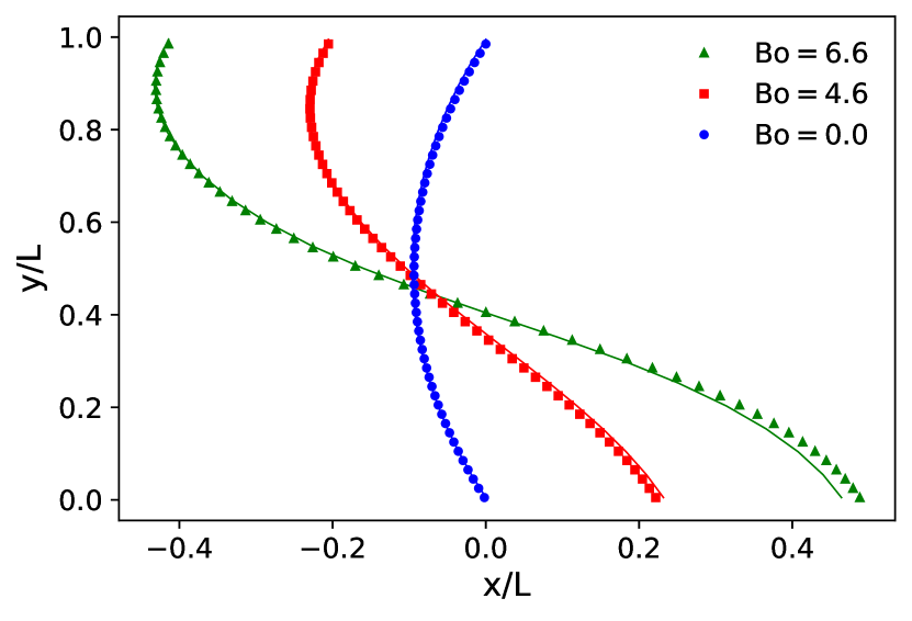
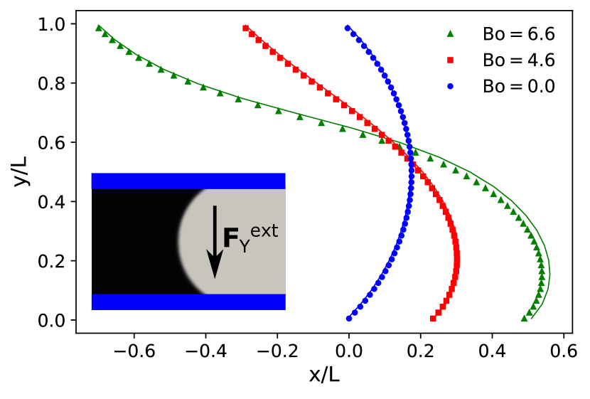
Figure 1: Interface shape for $\theta\approx 51^{\circ}$ (top) and $112^{\circ}$ (bottom) and three different Bond numbers. Symbols are simulation results, solid lines are the semi-analytical predictions for each Bond number. The inset shows a sketch of the system. Here $L=L_{Y}=200$.

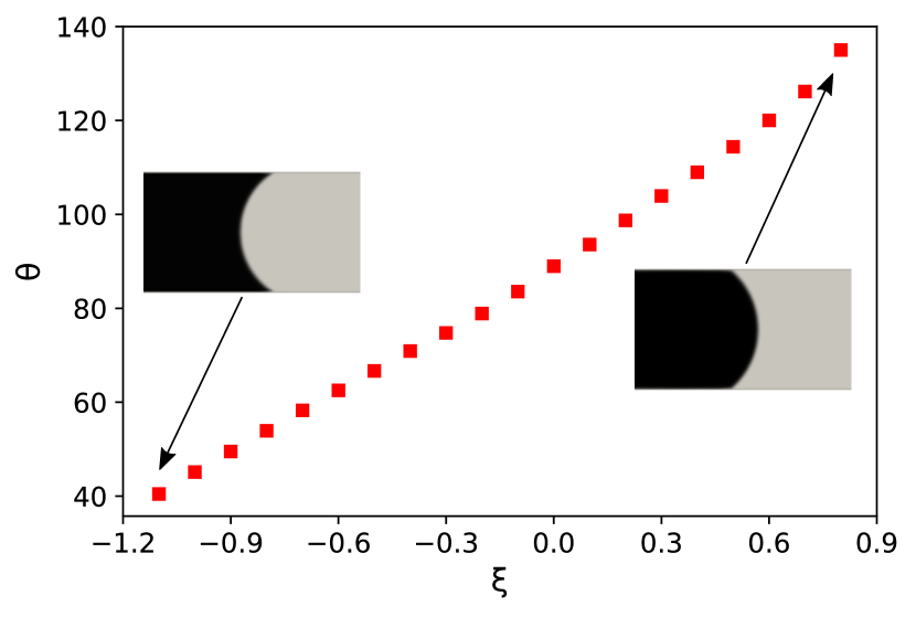
Figure 2: Mapping between the wetting parameter $\xi$ and the contact angle $\theta$ of the liquid bridge (in degrees). The insets show two examples of bridge shape for a hydrophilic and a hydrophobic substrate with wetting parameter and contact angle indicated by the arrows.

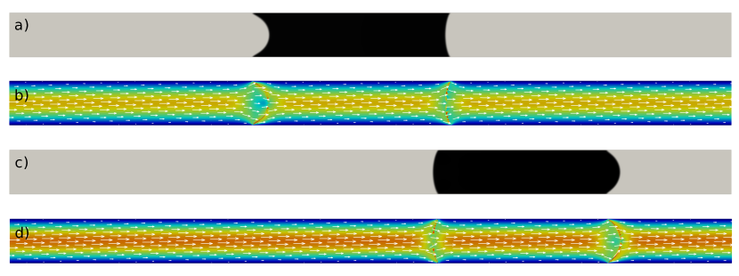
Figure 3: Example of two liquid bridges moving due to a force $F^{\tiny{\mbox{ext}}}=10^{-5}$ lattice units between (a) two hydrophilic substrates, with $\xi=-0.8$, and (c) two hydrophobic substrates, with $\xi=0.7$. Panels (b) and (d) show the velocity fields corresponding to panels (a) and (c) respectively, where the colours denote the velocity magnitude (red for fast and blue for slow) and the arrows indicate its direction. Note that the velocity is approximately the same for both fluids and that they are incompressible.

3.2 Force on substrates

We now analyze the fluid friction forces exerted on the substrates by a moving bridge. In order to make our results generic, we express them in terms of two non-dimensional quantities. The capillary number, ${\rm Ca}$, quantifies the relative importance of the viscous forces over the surface tension forces. In our simulations, since the surface tension is constant, ${\rm Ca}$ will be a measure of the bridge velocity. We define it as:

$${\rm Ca}=\frac{\langle\rho\rangle\langle u\rangle\nu}{\gamma},$$ (14)

where $\langle\rho\rangle$ is the average density in the simulation domain, and $\langle u\rangle$ is the average velocity of the fluid in the $x$-direction, which, as we have checked, is the same as the interface velocity of the liquid bridge in the steady state. The other non-dimensional quantity is the drag coefficient, ${\rm Cd}$, which is a measure of the drag, or frictional, force exerted by the liquid on the substrates:

$${\rm Cd}=\frac{F^{\tiny{\mbox{drag}}}}{\langle\rho\rangle\langle u\rangle^{2}L_{x}}.$$ (15)

By dimensional analysis, the drag force on the substrates is of the form $F^{\tiny{\mbox{drag}}}\propto\langle\rho\rangle\langle u\rangle\nu L_{x}$. Note that this is similar to Stokes’ law for a sphere immersed in a viscous fluid, with the sphere radius replaced by $L_{x}$ and a proportionality constant equal to $6\pi$. For the liquid bridges, the proportionality constant depends on the contact angle. We expect that the drag force will be smaller for hydrophobic substrates than for hydrophilic ones. Therefore

$${\rm Cd}\sim\frac{\langle\rho\rangle\nu^{2}}{\gamma}{\rm Ca^{-1}}.$$ (16)

We initialize the liquid bridges as described in section 3.1 and apply an external force in the direction $x$ parallel to the substrates. After an initial transient, whose duration depends on the contact angles and the magnitude of the applied force, a steady-state is established in which the bridge moves with a constant velocity. This requires that the drag force on the substrates must have equal magnitude to the force applied on the bridge, which provides a check on the consistency of our results. Figure 3 shows two examples of moving liquid bridges, between hydrophilic or hydrophobic substrates. The interfaces are set far enough apart that they do not interact with each other and a Poiseuille flow develops inside and outside the bridges. Only close to the interfaces are there disruptions to the velocity field. This occurs because the two fluids are immiscible, and therefore there is no relative velocity in the direction normal to the interface of the liquid bridge.

In figure 4, the expected power law ${\rm Cd}\propto{\rm Ca}^{-1}$ is confirmed, where the linear fits assume a slope of $-1$. We note that the hydrophilic substrate ($\xi=-0.8$) results in a greater drag force on the plates than the hydrophobic substrate ($\xi=0.7$) with the neutral wetting substrate ($\xi=0$) lying in between.

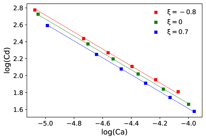
Figure 4: Plot of the drag coefficient ${\rm Cd}$ vs capillary number ${\rm Ca}$ for three wetting parameters $\xi$. The squares are simulation results, the solid lines are linear fits of the form $f(x)=-x+b$.

3.3 Dynamic contact angle

In this section, we measure the changes in contact angle when the bridge is moving, with respect to the bridge at rest. We consider three cases: same wetting parameter at both top, $\xi_{T}$, and bottom, $\xi_{B}$, substrates and ${\rm Bo}=0$; different wetting parameters at top and bottom and ${\rm Bo}=0$; and same wetting parameter at top and bottom but with ${\rm Bo}\neq 0$. We point out that the flow of liquid bridges is laminar: the Reynolds number, defined as ${\rm Re}=\langle u\rangle L_{Y}/\nu$, varies between $1.1$ and $3.1$.

3.3.1 Identical substrates, no gravity.

As illustrated in figure 3, the contact angles become different from those of the bridges at rest. Additionally, the angles of the advancing interface (on the right) increase while those of the retreating interface (on the left) decrease, for both hydrophilic and hydrophobic substrates. The top and bottom contact angles are the same if ${\rm Bo}=0$ and $\xi_{T}=\xi_{B}$ as here. In figure 5(a), we show how the angle changes as a function of ${\rm Ca}$ (varying velocities) for three different wetting parameters. We note that the slopes of $\Delta\theta$ for the advancing contact angles are always positive, but they might vary slightly with the wetting parameter and the slopes of $\Delta\theta$ for the receding contact angles are negative. Since $\Delta\theta\times{\rm Ca}$ is almost linear (except for receding angles with $\xi=-0.8$), we use the slope of a linear fit $\Delta\theta(x)=\alpha\,{\rm Ca}$ as a measure of the angles’ dependence on the wetting parameter. These slopes are shown in Figs. 5(b) and (c) for receding ($\alpha_{L}$) and advancing ($\alpha_{R}$) angles, respectively. (The fit of $\Delta\theta$ for receding angles with $\xi=-0.8$ did not use the four points with largest ${\it Ca}$). Slopes $\alpha_{L}$ vary more strongly with $\xi$ than $\alpha_{R}$. We note that $|\alpha_{L}|$ is larger for smaller equilibrium contact angles. This happens because the receding angles tend to decrease and this is easier if they are already small due to the tendency of the interface to become more curved for higher velocities. Curiously, $\alpha_{R}$ has a minimum close to $\xi=0$. This means that it is more difficult to change the interface shape when it is flat ($\theta=90^{\circ}$).

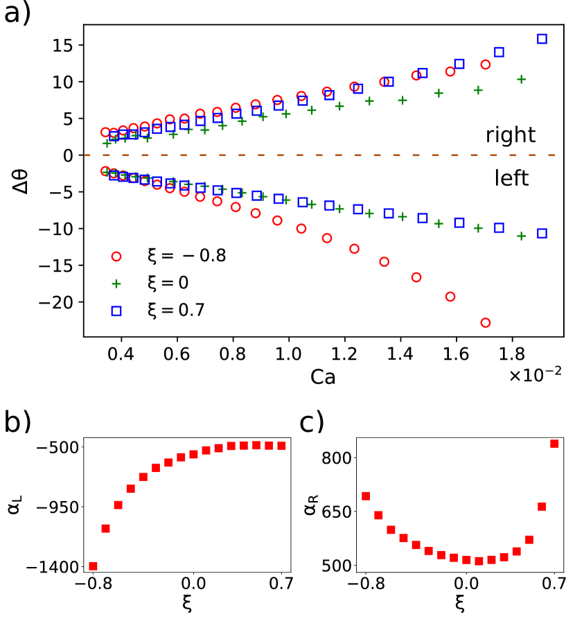
Figure 5: (a) Change in contact angle $\Delta\theta$ relative to equilibrium vs capillary number ${\rm Ca}$ for three wetting parameters $\xi$. $\Delta\theta>0$ for the advancing interface (on the right) and $\Delta\theta<0$ for the receding interface (on the left). The contact angles are the same at the top and bottom substrates. The slopes of the linear fits of $\Delta\theta$ vs ${\rm Ca}$ are plotted in (b) and (c) for the receding (left) and advancing (right) angles, respectively.

3.3.2 Different substrates, no gravity.

Here we consider different wetting parameters at the top and bottom substrates, $\xi_{T}$ and $\xi_{B}$ respectively. We proceed as in section 3.3.1 and apply an external force in the direction parallel to the flow. Then we relate the change $\Delta\theta$ to the capillary number ${\rm Ca}$ and measure the slope of the linear fit for each combination of $\xi_{T}$ and $\xi_{B}$, see in figure 6. Because the bridge is moving and the top and bottom wettabilities are different, all four contact angles are different and their slopes are shown separately. For the contact angles on the right (advancing), the slopes vary over a narrower range, and therefore the errors of the linear fits and other numerical errors in contact angle measurements are more visible. These figures have a symmetry: the bottom angle on each side (left and right) for a given combination $\xi_{T}=\xi_{1}$ and $\xi_{B}=\xi_{2}$ is the same as the top angle on the same side with exchanged parameters $\xi_{T}=\xi_{2}$ and $\xi_{B}=\xi_{1}$. This does not hold for ${\rm Bo\neq 0}$ since the force in the $y$ direction breaks the top-bottom symmetry. For the angles on the left, which vary over a wider range, the slopes of the fits are only weakly affected by the wetting on the bottom substrate and vice-versa. Hydrophilic substrates ($\xi<0$) yield larger absolute slopes on the left-hand side. For the angles on the right, the slopes are smaller close to neutral wetting ($\xi=0$).

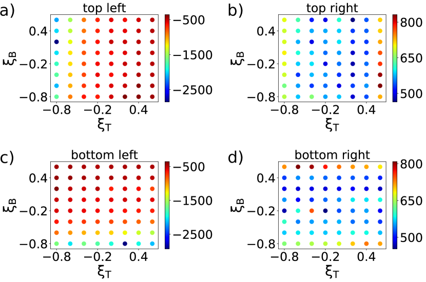
Figure 6: Slopes of the linear fits of $\Delta\theta$ vs ${\rm Ca}$ for the four contact angles of the liquid bridge with different wetting parameters at top and bottom, $\xi_{T}$ and $\xi_{B}$ respectively.

3.3.3 Identical substrates, ${\rm Bo}\neq 0$.

Now we consider bridges with the same wetting parameter at top and bottom but with an external force (e.g., gravity) perpendicular to the plates. We measure the contact angle change $\Delta\theta$ as a function of the capillary number $Ca$ as before. Figure 7 shows the variations of the four angles for three different Bond numbers and two wetting parameters. The external force in the $y$ direction increases some angles and decreases others. Those angles that decrease on the left interface vary more strongly with capillary number than those on the right interface. For instance, the top left (TL) angle increases for a hydrophilic top substrate as ${\rm Bo}$ increases. Thus, its variation with ${\rm Ca}$ is smaller for larger ${\rm Bo}$ as shown in figure 7(a). The opposite happens for a hydrophobic top substrate: as the TL angle decreases with ${\rm Bo}$, its variation with ${\rm Ca}$ is greater for larger ${\rm Bo}$. The same analysis holds for the other three angles.

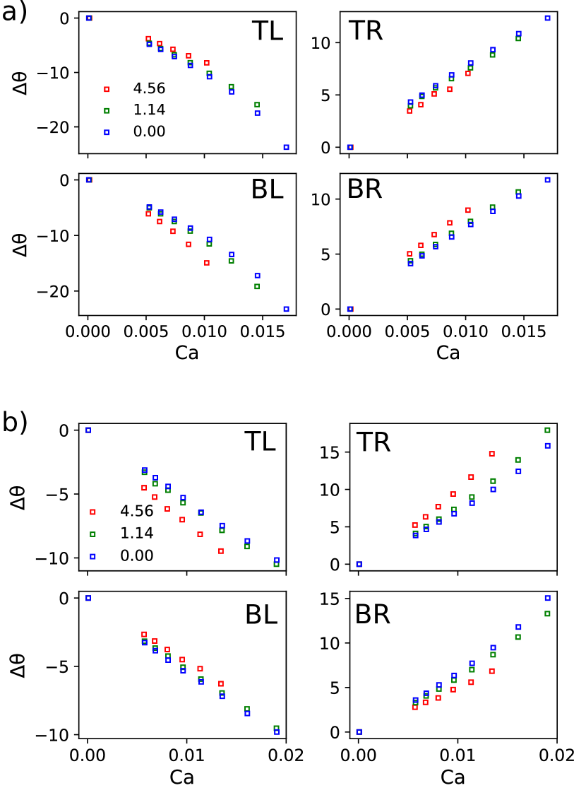
Figure 7: Changes in contact angles $\Delta\theta$ vs capillary number ${\rm Ca}$ for different Bond numbers (see legend: top left (TL), top right (TR), bottom left (BL), bottom right (BR). The wetting parameter is the same on the top and bottom substrates: (a) $\xi=-0.8$ and (b) $\xi=0.7$.

3.4 Breaking bridges

In this section we examine the maximum capillary number ${\rm Ca}_{\tiny{\mbox{max}}}$ for which the liquid bridge is stable and does not break. Thus, using the same setup as in the previous sections, we simulate bridges with larger external forces applied in the $x$ direction to observe bridge rupture. We say the bridge has broken if, after a long enough time ($t=5\times 10^{5}$), there is no possible path inside the liquid bridge component connecting the top and bottom substrates.

Figure 8(a) shows ${\rm Ca}_{\tiny{\mbox{max}}}$ for liquid bridges between identical substrates and different Bond numbers. We notice that bridges with wetting parameters around $\xi=0$ (neutral wetting) are, in general, more stable for any ${\rm Bo}$. This is because the interface is straight for $\xi=0$ and increasing ${\rm Bo}$ does not much affect its shape. Bridges between hydrophilic substrates are also more resilient, presumably owing to the larger liquid-solid contact area that provides greater adhesion. Increasing ${\rm Bo}$ makes bridges more unstable, especially far from $\xi=0$. To have an idea of what these numbers mean in physical units, let us consider a liquid bridge made of a commercially available aqueous surfactant solution (Pustefix, Germany) in air, for which $\Delta\rho\sim 10^{3}$ kg m^-3, $\gamma\sim 28$ mJ m^-2 and $\nu\sim 10^{-6}$ m² s^-1. For $\xi=-0.6$ and ${\rm Bo}=1.1$, which corresponds to $L_{y}=1.8$ mm, the maximum capillary number is ${\rm Ca}_{\tiny{\mbox{max}}}\approx 0.1$, which gives a bridge velocity of $3$ m/s. In this case, the drag coefficient is ${\rm Cd}=0.95$, whence the drag force on the plates is $250$ N. For the same $\xi$ and ${\rm Bo}=6.8$, which corresponds to $L_{y}=4.6$ mm, ${\rm Ca}_{\tiny{\mbox{max}}}\approx 0.012$, which gives a velocity of $0.36$ m/s. The drag coefficient in this case is ${\rm Cd}=9.1$ and the corresponding drag force is $87$ N. Finally, note that, according to our earlier work [11], the maximum span of a liquid bridge at equilibrium is four capillary lengths.

In figure 8(b), we plot ${\rm Ca}_{\tiny{\mbox{max}}}$ for bridges with ${\rm Bo}=0$, but different wetting parameters at top and bottom. Bridges with $\xi_{T}\neq\xi_{B}$ are more unstable, which effect is stronger close to the extremes, with $\xi_{T}=0.6$ and $\xi_{B}=-0.6$ and $\xi_{T}=-0.6$ and $\xi_{B}=0.6$.

It is interesting to note that, in all cases considered here, the smallest capillary number for which a bridge breaks is less than that needed to break a thin liquid lamella, ${\rm Ca}\sim 0.26$ [22].

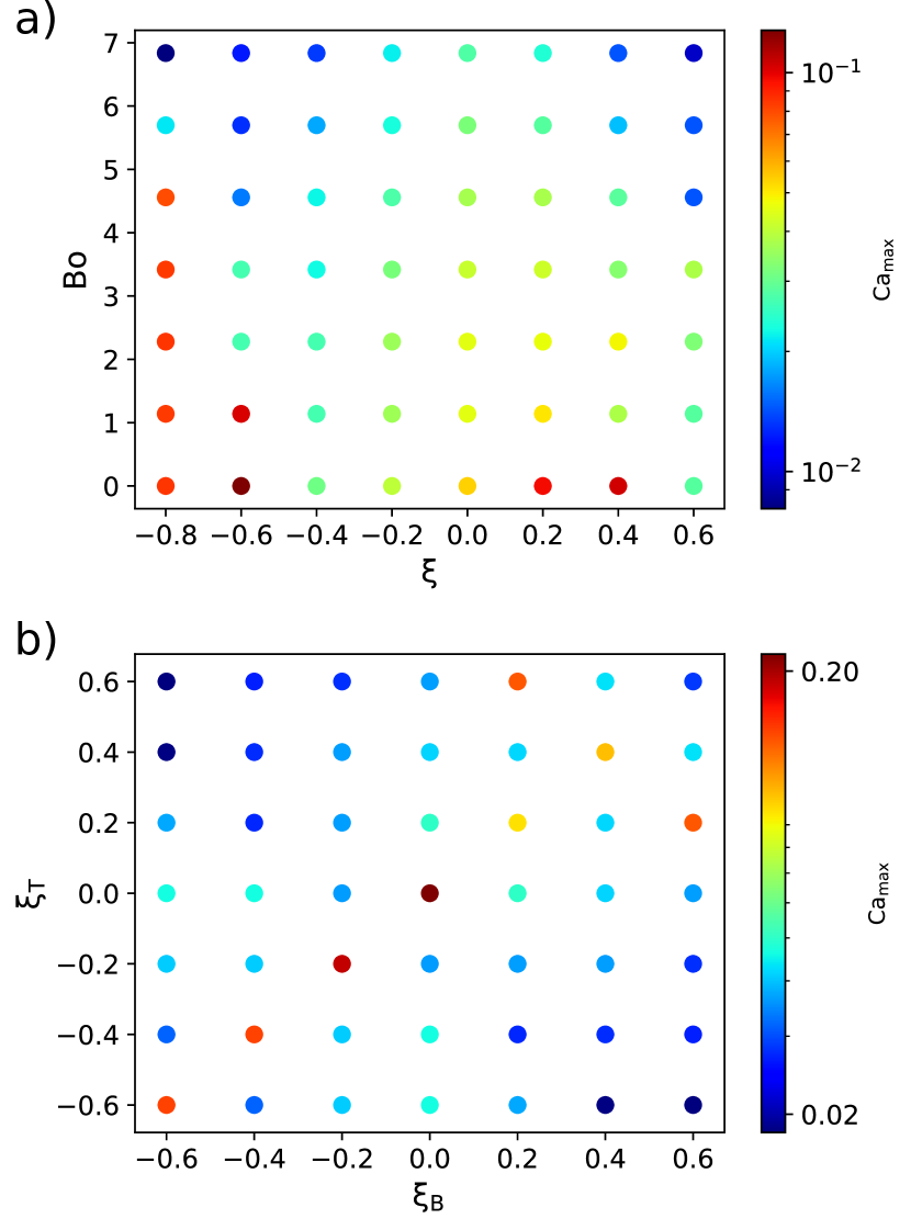
Figure 8: Maximum capillary number ${\rm Ca}_{\tiny{\mbox{max}}}$ for which the liquid bridge does not break. (a) Same wetting parameter $\xi$ at top and bottom substrates and varying Bond number ${\rm Bo}$. (b) ${\rm Bo}=0$ and different wetting parameters on top and bottom.

4 Conclusions

We have simulated the motion of a two-dimensional liquid bridge sandwiched between flat horizontal substrates of tunable wettability, using the lattice Boltzmann method. This was validated by comparison with quasi-analytic results for equilibrium (static) bridges [11], and found to be reliable except for Bond numbers very close to the maximum above which an equilibrium bridge breaks.

For steady-state bridges moving between identical substrates, ${\rm Cd}\sim{\rm Ca}^{-1}$ as required by dimensional analysis. However the prefactor depends on the liquid contact angles, being larger for hydrophilic than for hydrophobic substrates. This accords with the intuitive expectation that bridges of a given volume should have a larger contact area with a hydrophilic than with a hydrophobic substrate, thus leading to higher drag in the former case than in the latter. The effect is, however, not very pronounced: drag reduction due to hydrophobicity is at most about $20\%$.

Moving bridges deform from their equilibrium shapes. We quantified this by measuring the deviations of contact angles from their equilibrium values. For not-too-fast moving bridges these deviations are proportional to the capillary number with slopes that are always negative on the receding side of a bridge and positive on the advancing side, but exhibit a complex dependence on the contact angles.

Finally, we investigated bridge stability by mapping the largest capillary number for which a bridge will not break, for given contact angles at the top and bottom substrates and given Bond number. Interestingly, the most stable bridges appear to be those with equilibrium contact angles around $90^{\circ}$. Stability (i.e, breakup deferred to larger ${\rm Ca}$) is also favoured by hydrophilicity and small Bond numbers.

One possible area of future research would be the detailed breakup of bridges, either as a result of increasing their velocity (i.e., ${\rm Ca}$) or substrate separation (i.e., ${\rm Bo}$). One possible extension would be to non-Newtonian fluids, which occur in many industrial and biological contexts.

References

- [1] J. N. Israelachvili. Intermolecular and Surface Forces. Elsevier, Inc.,, Amsterdam, third edition, 2011.
- [2] M. Pakpour, M. Habib, P. Møller, and D. Bonn. How to construct the perfect sandcastle. Scientific Reports, 2:545, 2012.
- [3] Y. Men, X. Zhang, and W. Wang. Capillary liquid bridges in atomic force microscopy (afm): Formation, rupture, and hysteresis. J. Chem. Phys., 131:184702, 2009.
- [4] R. B. Edwards. Joint tolerances in capillary copper piping joints. Welding Journal, 6:321–324, 1972.
- [5] L. Vagharchakian, F. Restagno, and L. Léger. Capillary bridge formation and breakage: a test to characterize antiadhesive surfaces. J. Phys. Chem. B, 113:3769–3775, 2009.
- [6] A. M. Alencar, A. Majumdar, Z. Hantos, S. V. Buldyrev, H. E. Stanley, and B. Suki. Crackles and instabilities during lung inflation. Physica A, 357:18–26, 2005.
- [7] B. N. Persson. Wet adhesion with application to tree frog adhesive toe pads and tires. J. Phys.: Condens. Matter, 19:376110, 2007.
- [8] M. Prakash, D. Queré, and J. W. M. Bush. Surface tension transport of prey by feeding shorebirds: The capillary ratchet. Science, 320:931–934, 2008.
- [9] E. W. Washburn. The dynamics of capillary flow. Phys. Rev., 17:273–283, 1921.
- [10] N. Nagy. Contact angle determination on hydrophilic and superhydrophilic surfaces by using -type capillary bridges. Langmuir, 35:5202–5212, 2019.
- [11] P. I. C. Teixeira and M. A. C. Teixeira. The shape of two-dimensional liquid bridges. J. Phys.: Condens. Matter, 32(3):034002, oct 2019.
- [12] P. D. Howell, S. L. Waters, and J. B. Grotberg. The propagation of a liquid bolus along a liquid-lined flexible tube. J. Fluid Mech., 406:309–335, 2000.
- [13] C. N. Baroud, F. Gallaire, and R. Dangla. Dynamics of microfluidic droplets,. La. Chip, 10:2032–2045, 2010.
- [14] D. Halpern, H. Fujioka, S. Takayama, and J. B. Grotberg. Respir. Physiol. Neurobiol., 163:222–231, 2008.
- [15] X. Shan and H. Chen. Lattice boltzmann model for simulating flows with multiple phases and components. Phys. Rev. E, 47:1815–1819, Mar 1993.
- [16] T. Krüger, H. Kusumaatmaja, A. Kuzmin, O. Shardt, G. Silva, and E. Magnus Viggen. The Lattice Boltzmann Method - Principles and Practice. Springer International Publishing, 10 2016.
- [17] R. C. V. Coelho and M. M. Doria. Lattice boltzmann method for semiclassical fluids. Computers & Fluids, 165:144 – 159, 2018.
- [18] Z. Guo, C. Zheng, and B. Shi. Discrete lattice effects on the forcing term in the lattice boltzmann method. Phys. Rev. E, 65.
- [19] R. C. V. Coelho, C. B. Moura, M. M. Telo da Gama, and N. A. M. Araújo. Wetting boundary conditions for multicomponent pseudopotential lattice boltzmann. Int. J. Numer. Methods Fluids, 93(8):2570–2580, 2021.
- [20] M. Sedahmed, R. C. V. Coelho, and H. A. Warda. An improved multicomponent pseudopotential lattice boltzmann method for immiscible fluid displacement in porous media. Physics of Fluids, 34(2):023102, 2022.
- [21] R. Mei, D. Yu, W. Shyy, and L.S. Luo. Force evaluation in the lattice boltzmann method involving curved geometry. Phys. Rev. E, 65.
- [22] I. Cantat. Liquid meniscus friction on a wet plate: Bubbles, lamellae, and foams. Phys. Fluids, 25.