A PTAS for Capacitated Vehicle Routing on Trees

Abstract

We give a polynomial time approximation scheme (PTAS) for the unit demand capacitated vehicle routing problem (CVRP) on trees, for the entire range of the tour capacity. The result extends to the splittable CVRP.

1 Introduction

Given an edge-weighted graph with a vertex called depot, a subset of vertices with demands, called terminals, and an integer tour capacity $k$, the capacitated vehicle routing problem (CVRP) asks for a minimum length collection of tours starting and ending at the depot such that those tours together cover all the demand and the total demand covered by each tour is at most $k$. In the unit demand version, each terminal has unit demand, which is covered by a single tour; in the splittable version, each terminal has a positive integer demand and the demand at a terminal may be covered by multiple tours.

The CVRP was introduced by Dantzig and Ramser in 1959 [DR59] and is arguably one of the most important problems in Operations Research. Books have been dedicated to vehicle routing problems, e.g., [TV02, GRW08, CL12, AGM16]. Yet, these problems remain challenging, both from a practical and a theoretical perspective.

Here we focus on the special case when the underlying metric is a tree. That case has been the object of much research. The splittable tree CVRP was proved NP-hard in 1991 [LLM91], so researchers turned to approximation algorithms. Hamaguchi and Katoh [HK98] gave a simple lower bound: every edge must be traversed by enough tours to cover all terminals whose shortest paths to the depot contain that edge. Based on this lower bound, they designed a 1.5-approximation in polynomial time [HK98]. The approximation ratio was improved to $(\sqrt{41}-1)/4$ by Asano, Katoh, and Kawashima [AKK01] and further to $4/3$ by Becker [Bec18], both results again based on the lower bound from [HK98]. On the other hand, it was shown in [AKK01] that using this lower bound one cannot achieve an approximation ratio better than $4/3$. More recently, researchers tried to go beyond a constant factor so as to get a $(1+\epsilon)$-approximation, at the cost of relaxing some of the constraints. When the tour capacity is allowed to be violated by an $\epsilon$ fraction, there is a bicriteria PTAS for the unit demand tree CVRP due to Becker and Paul [BP19]. When the running time is allowed to be quasi-polynomial, Jayaprakash and Salavatipour [JS22] very recently gave a quasi-polynomial time approximation scheme (QPTAS) for the unit demand and the splittable versions of the tree CVRP. In this paper, we close this line of research by obtaining a $(1+\epsilon)$-approximation without relaxing any of the constraints – in other words, a polynomial-time approximation scheme (PTAS).

Theorem 1.

There is an approximation scheme for the unit demand capacitated vehicle routing problem (CVRP) on trees with polynomial running time.

Corollary 2.

There is an approximation scheme for the splittable capacitated vehicle routing problem (CVRP) on trees with running time polynomial in the number of vertices $n$ and the tour capacity $k$.

To the best of our knowledge, this is the first PTAS for the CVRP in a non-trivial metric and for the entire range of the tour capacity. Previously, PTASs for small capacity as well as QPTASs were given for the CVRP in several metrics, see Section 1.1.3.

1.1 Related Work

Our algorithms build on [JS22] and [BP19] but with the addition of significant new ideas, as we now explain.

1.1.1 Comparison with the QPTAS in [JS22]

Jayaprakash and Salavatipour noted in [JS22] that

“it is not clear if it (the QPTAS) can be turned into a PTAS without significant new ideas.”

The running time in [JS22] is $n^{O_{\epsilon}(\log^{4}n)}$. Where do those four $\log n$ factors in the exponent come from? At a high level, the QPTAS in [JS22] consists of three parts: (1) reducing the height of the tree; (2) designing a bicriteria QPTAS; (3) going from the bicriteria QPTAS to a true QPTAS. Our approach builds on [JS22] but differs from it in each of the three parts, so that in the end we get rid of all of four $\log n$ factors, hence a PTAS.

(1) Jayaprakash and Salavatipour [JS22] reduce the input tree height from $O(n)$ to $O_{\epsilon}(\log^{2}n)$; whereas instead of the input tree, we consider a tree of components (Lemma 9) and reduce its height to $O_{\epsilon}(1)$, see Fig. 1. Pleasingly, the height reduction (Section 4) is much simpler than in [JS22]. The analysis differs from [JS22] and uses the structure of a near-optimal solution established in Section 3 and the bounded distance property (Definition 3 and Theorem 5).

(2) In the adaptive rounding used in [JS22], they consider the entire range $[1,k]$ of the demands of subtours and partition the subtour demands into buckets, resulting in $\Omega_{\epsilon}(\log k)$ different subtour demands after rounding. In our approach, we define large and small subtours inside components, depending on whether their demands are $\Omega_{\epsilon}(k)$ (Definition 14). Then we transform the solution structure to eliminate small subtours (Section 3), hence only $O_{\epsilon}(1)$ different subtour demands after rounding. This elimination requires a delicate handling of small subtours. Thanks to the additional structure, our analysis of the adaptive rounding is simpler than in [JS22], and in particular, we do not need the concept of buckets.

(3) Jayaprakash and Salavatipour show that the orphan tokens, which are removed from the tours exceeding capacity, can probably be covered by duplicating a small random set of tours in the optimal solution. Their approach requires remembering the demands of $\Omega(\log n)$ subtours passing through each edge. To avoid this $\Omega(\log n)$ factor, our approach to cover the orphan tokens (Section 3.1) is different, see Fig. 2. The analysis of our approach (Sections 3.2 and 3.3) contains several novelties of this paper.

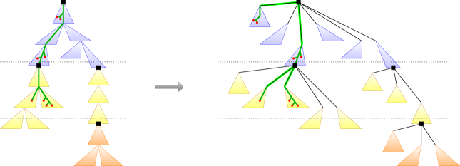
Figure 1: Height reduction for a tree of components. The left figure represents the initial tree of components, where each triangle represents a component. We partition the components into classes (indicated by blue, yellow, and orange), according to the distances from the roots of the components to the root of the tree, and we reduce the height within each class to 1 (right figure), see Section 4. The thick green path in the left figure represents a tour in an optimal solution. The red circular nodes are the terminals visited by that tour. The corresponding tour in the new tree (right figure) spans the same set of terminals.

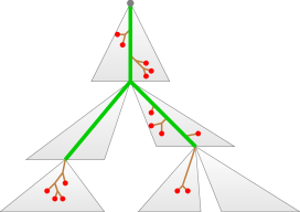
(a)

(b)

Figure 2: Covering the orphan tokens (in red). In Fig. 2(a), the orphan tokens are contained in the small pieces (in brown) that are removed from the tours exceeding capacity. We add the thick paths (in green) to connect all of the small pieces to the root of the tree. The cost of the thick paths is an $O(\epsilon)$ fraction of the optimal cost (Lemmas 17 and 18), thanks to the bounded distance property. The induced traveling salesman tour is a double cover of the tree spanning the orphan tokens. Next, we apply the iterated tour partitioning (ITP) algorithm on that tour. In Fig. 2(b), the two paths (in blue and in orange) represent the connections to the depot added by the ITP algorithm. Their cost is again an $O(\epsilon)$ fraction of the optimal cost (Lemma 19), thanks to the bound on the number of orphan tokens and the bounded distance property.

1.1.2 Comparison with the Bicriteria PTAS in [BP19]

Why is the algorithm in [BP19] a bicriteria PTAS, but not a PTAS?

Becker and Paul [BP19] start by decomposing the tree into clusters. (1) They require that each leaf cluster is visited by a single tour. When the violation of the tour capacity is not allowed, this requirement does not preserve a $(1+\epsilon)$-approximate solution, see Fig. 5. (2) They also require that each small internal cluster is visited by a single tour. To that end, they modify the optimal solution by reassigning all terminals of a small cluster to some existing tour at the cost of possibly violating the tour capacity. Such modifications do not seem achievable in the design of a PTAS.

In this paper, we start by defining components (Lemma 9), inspired by clusters in [BP19]. Unlike [BP19], we allow terminals in any component to be visited by multiple tours. However, allowing many subtours inside a component could result in an exponential running time for a dynamic program. To prevent that, we modify the solution structure inside a component so that the number of subtours becomes bounded (Theorem 13). Instead of considering all subtours simultaneously as in [BP19], we distinguish small subtours from large subtours (Definition 14). Inspired by [BP19], we combine small subtours and reallocate them to existing tours such that the violation of the tour capacity is an $O(\epsilon)$ fraction, see Steps 1 to 3 of the construction in Section 3.1. Next, we use the iterated tour partitioning (ITP) and its postprocessing to reduce the demand of the tours exceeding capacity (Fig. 2), which is a novelty in this paper, see Steps 4 to 6 of the construction in Section 3.1. The ITP algorithm and its postprocessing are analyzed in Sections 3.2 and 3.3. In particular, we bound the cost due to the ITP algorithm thanks to the bounded distance property (Theorem 5) and to the parameters in our component decomposition that are different from those in [BP19], see Remark 10. Besides the above novelties in our approach, the height reduction (Fig. 1, see also Section 4), the adaptive rounding (Section 5), the reduction to bounded distances (Section 7), as well as part of the dynamic program (Section 6) are new compared with [BP19]. These additional techniques are essential in the design of our PTAS, because of the more complicated solution structure inside components in our approach compared with the solution structure inside clusters in [BP19].

1.1.3 Other Related Work

Constant-factor approximations in general metric spaces.

The CVRP is a generalization of the traveling salesman problem (TSP). In general metric spaces, Haimovich and Rinnooy Kan [HR85] introduced a simple heuristics, called iterated tour partitioning (ITP). Altinkemer and Gavish [AG90] showed that the approximation ratio of the ITP algorithm for the unit demand and the splittable CVRP is at most $1+\left(1-\frac{1}{k}\right)C_{\mathrm{TSP}}$, where $C_{\mathrm{TSP}}\geq 1$ is the approximation ratio of a TSP algorithm. Bompadre, Dror, and Orlin [BDO06] improved this bound to $1+\left(1-\frac{1}{k}\right)C_{\mathrm{TSP}}-\Omega\left(\frac{1}{k^{3}}\right)$. The ratio for the unit demand and the splittable CVRP on general metric spaces was recently improved by Blauth, Traub, and Vygen [BTV21] to $1+C_{\mathrm{TSP}}-\epsilon$, for some small constant $\epsilon>0$.

QPTASs.

Das and Mathieu [DM15] designed a QPTAS for the CVRP in the Euclidean space; Jayaprakash and Salavatipour [JS22] designed a QPTAS for the CVRP in trees and extended that algorithm to QPTASs in graphs of bounded treewidth, bounded doubling or highway dimension. When the tour capacity is fixed, Becker, Klein, and Saulpic [BKS17] gave a QPTAS for planar graphs and bounded-genus graphs.

PTASs for small capacity.

In the Euclidean space, there have been PTAS algorithms for the CVRP with small capacity $k$: work by Haimovich and Rinnooy Kan [HR85], when $k$ is constant; by Asano et al. [AKTT97] extending techniques in [HR85], for $k=O(\log n/\log\log n)$; and by Adamaszek, Czumaj, and Lingas [ACL10], when $k\leq 2^{\log^{f(\epsilon)}(n)}$. For higher dimensional Euclidean metrics, Khachay and Dubinin [KD16] gave a PTAS for fixed dimension $\ell$ and $k=O(\log^{\frac{1}{\ell}}(n))$. Again when the capacity is bounded, Becker, Klein and Schild [BKS19] gave a PTAS for planar graphs; Becker, Klein, and Saulpic [BKS18] gave a PTAS for graphs of bounded highway dimension; and Cohen-Addad et al. [CFKL20] gave PTASs for bounded genus graphs and bounded treewidth graphs.

Unsplittable CVRP.

In the unsplittable version of the CVRP, every terminal has a positive integer demand, and the entire demand at a terminal should be served by a single tour. On general metric spaces, the best-to-date approximation ratio for the unsplittable CVRP is roughly $3.194$ due to the recent work of Friggstad et al. [FMRS21]. For tree metrics, the unsplittable CVRP is APX-hard: indeed, it is NP-hard to approximate the unsplittable tree CVRP to better than a 1.5 factor [GW81] using a reduction from the bin packing problem. Labbé, Laporte and Mercure [LLM91] gave a 2-approximation for the unsplittable tree CVRP. The approximation ratio for the unsplittable tree CVRP was improved to $(1.5+\epsilon)$ very recently by Mathieu and Zhou [MZ22], building upon several techniques in the current paper.

1.2 Overview of Our Techniques

The main part of our work focuses on the unit demand tree CVRP, and we extend our results to the splittable tree CVRP in the end of this work.

Definition 3 (bounded distances).

Let $D_{\min}$ (resp. $D_{\max}$) denote the minimum (resp. maximum) distance between the depot and any terminal in the tree. We say that an instance has bounded distances if $D_{\max}<\left(\frac{1}{\epsilon}\right)^{\frac{1}{\epsilon}-1}\cdot D_{\min}.$

Theorem 1 follows directly from Theorems 4 and 5.

Theorem 4.

There is a polynomial time $(1+4\epsilon)$-approximation algorithm for the unit demand CVRP on the tree $T$ with bounded distances.

Theorem 5.

For any $\rho\geq 1$, if there is a polynomial time $\rho$-approximation algorithm for the unit demand (resp. splittable, or unsplittable) CVRP on trees with bounded distances, then there is a polynomial time $(1+5\epsilon)\rho$-approximation algorithm for the unit demand (resp. splittable, or unsplittable) CVRP on trees with general distances.

Theorem 5 may be of independent interest for the splittable and the unsplittable versions of the tree CVRP.

Outline of the PTAS for unit demand instances with bounded distances (Theorem 4).

In Sections 3, 4 and 5, we show that there exists a near-optimal solution with a simple structure, and in Section 6, we use a dynamic program to compute the best solution with that structure.

In Section 3, we consider the components of the tree $T$ (Lemma 9) and we show that there exists a near-optimal solution such that terminals within each component are visited by a constant $O_{\epsilon}(1)$ number of tours and that each of those tours visits $\Omega_{\epsilon}(k)$ terminals in that component (Theorem 13). The proof of Theorem 13 contains several novelties in our work. We start by defining large and small subtours inside a component, depending on the number of terminals visited by the subtours. To construct a near-optimal solution with that structure, first, we detach small subtours from their initial tours, combine small subtours in the same component, and reallocate the combined subtours to existing tours. Then we remove subtours from tours exceeding capacity. To connect the removed subtours to the root of the tree, we include the spines subtours (Definition 12) of all internal components, and we obtain a traveling salesman tour. Next, we apply the iterated tour partitioning (ITP) algorithm on that tour, see Fig. 2. Finally, in a postprocessing step, we eliminate the small subtours created due to the ITP algorithm. The complete construction is in Section 3.1; the feasibility of the construction is in Section 3.2; and the analysis on the constructed solution is in Section 3.3, which in particular uses the bounded distance property.

In Section 4, we transform the tree $T$ into a tree $\hat{T}$ that has $O_{\epsilon}(1)$ levels of components (Fig. 1) and satisfies the following property.

Fact 6.

The tree $\hat{T}$ defined in Section 4 can be computed in polynomial time. The components in the tree $\hat{T}$ are the same as those in the tree $T$. Any solution for the unit demand CVRP on the tree $\hat{T}$ can be transformed in polynomial time into a solution for the unit demand CVRP on the tree $T$ without increasing the cost.

Thanks to the structure of the near-optimal solution on $T$ (Section 3) and to the bounded distance property, the optimal cost for $\hat{T}$ is increased by an $O(\epsilon)$ fraction compared with the optimal cost for $T$ (Theorem 23).

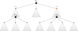
Figure 3: At each vertex of the tree, the dynamic program memorizes the capacities used by the subtours in the subtree and their total cost. Terminals within each component are visited by $O_{\epsilon}(1)$ tours and each of those tours visits $\Omega_{\epsilon}(k)$ terminals in that component. Here is an example of the flow of execution in the dynamic program. First, independent computation in each component (Algorithm 2). Next, computation in the subtrees rooted at vertices $v_{4}$ and $v_{5}$ (Algorithm 4). Then computation for the subtrees rooted at vertices $v_{2}$ and $v_{3}$ (Algorithm 3). Finally, computation for the subtree rooted at vertex $v_{1}$ (Algorithm 4). The output is the best solution in the subtree rooted at $v_{1}$. Vertices $v_{1},v_{4}$, and $v_{5}$, whose degrees may be arbitrarily large, are where adaptive rounding of the subtour demands is needed to maintain polynomial time (Algorithm 4). The cost due to the rounding is small thanks to the way components are defined and the bounded distance property, and does not accumulate excessively because the height is bounded (Section 4).

In Section 5, we apply the adaptive rounding on the demands of the subtours in a near-optimal solution on $\hat{T}$. Recall that in the design of the QPTAS by Jayaprakash and Salavatipour [JS22], the main technique is to show the existence of a near-optimal solution in which the demand of a subtour can be rounded to the nearest value from a set of only poly-logarithmic threshold values. In our work, we reduce the number of threshold values to a constant $O_{\epsilon}(1)$ (Theorem 26). To analyze the adaptive rounding, observe that an extra cost occurs whenever we detach a subtour and complete it into a separate tour by connecting it to the depot. We bound the extra cost thanks to the structure of a near-optimal solution inside components (Section 3), the reduced height of the components (Section 4), as well as the bounded distance property.

In Section 6, we design a polynomial-time dynamic program that computes the best solution on the tree $\hat{T}$ that satisfies the constraints on the solution structure imposed by previous sections. The algorithm combines a dynamic program inside components (Section 6.1) and two dynamic programs in subtrees (Section 6.2), see Fig. 3. Thus we obtain the following Theorem 7.

Theorem 7.

Consider the unit demand CVRP on the tree $\hat{T}$. There is a dynamic program that computes in polynomial time a solution with cost at most $(1+4\epsilon)\cdot\mathrm{opt}$, where $\mathrm{opt}$ denotes the optimal cost for the unit demand CVRP on the tree $T$.

Theorem 4 follows directly from Theorem 7 and 6.

Reduction from general distances to bounded distances (Theorem 5).

In Section 7, we prove Theorem 5. We use Baker’s technique to split tours into pieces such that each piece covers terminals that are within a certain range of distances from the depot. This requires duplicating some parts of the tours so that each piece of the tour is connected to the depot.

Extension to the splittable setting (Corollary 2).

In Section 8, we extend the result in Theorem 1 to the splittable setting, thus obtaining Corollary 2.

Open questions.

Previously, Jayaprakash and Salavatipour [JS22] extended their QPTAS on trees to QPTASs on graphs of bounded treewidth and beyond, including Euclidean spaces. While some of our techniques extend to those settings, others do not seem to carry over without significant additional ideas, so it is an interesting open question whether the techniques in our paper could be used in the design of PTAS algorithms for other metrics, such as graphs of bounded treewidth, planar graphs, and Euclidean spaces.

2 Preliminaries

Let $T$ be a rooted tree $(V,E)$ with root $r\in V$ and edge weights $w(u,v)\geq 0$ for all $(u,v)\in E$. The root $r$ represents the depot of the tours. Let $n$ denote the number of vertices in $V$. Let $V^{\prime}\subseteq V$ denote the set of terminals, such that a token is placed on each terminal $v\in V^{\prime}$. Let $k\in[1,n]$ be an integer capacity of the tours. The cost of a tour $t$, denoted by $\mathrm{cost}(t)$, is the overall weight of the edges on that tour. We say that a tour visits a terminal $v\in V^{\prime}$ if the tour picks up the token at $v$.

Definition 8 (unit demand tree CVRP).

An instance of the unit demand version of the capacitated vehicle routing problem (CVRP) on trees consists of

• an edge weighted tree $T=(V,E)$ with $n=|V|$ and with root $r\in V$ representing the depot,

• a set $V^{\prime}\subseteq V$ of terminals,

• a positive integer tour capacity $k$ such that $k\leq n$.

A feasible solution is a set of tours such that

• each tour starts and ends at $r$,

• each tour visits at most $k$ terminals,

• each terminal is visited by one tour.

The goal is to find a feasible solution such that the total cost of the tours is minimum.

Let $\mathrm{OPT}$ (resp. $\mathrm{OPT}_{1}$, $\mathrm{OPT}_{2}$, or $\mathrm{OPT}_{3}$) denote an optimal (resp. near-optimal) solution to the unit demand CVRP, and let $\mathrm{opt}$ (resp. $\mathrm{opt}_{1}$, $\mathrm{opt}_{2}$, or $\mathrm{opt}_{3}$) denote the value of that solution.

Without loss of generality, we assume that every vertex in the input tree $T$ has exactly two children, and that the terminals are the same as the leaf vertices of the tree. Indeed, general instances can be reduced to instances with these properties by inserting edges of weight 0, removing leaf vertices that are not terminals, and slicing out internal vertices of degree two, see, e.g. [BP19] for details.

For any vertex $v\in V$, a subtour at the vertex $v$ is a path that starts and ends at $v$ and only visits vertices in the subtree rooted at $v$. The demand of a subtour is the number of terminals visited by that subtour. For each vertex $v\in V$, let $\mathrm{dist}(v)$ denote the distance between $v$ and the depot in the tree $T$. For technical reasons, we allow dummy terminals to be included in the solution at internal vertices of the tree.

Throughout the paper, we define several constants depending on $\epsilon$: $\Gamma$ (Lemma 9), $\alpha$ (Theorem 13), $H_{\epsilon}$ (Lemma 21), and $\beta$ (Theorem 26). They satisfy the relation that $H_{\epsilon}\gg\Gamma\gg 1\gg\epsilon\gg\alpha\gg\beta$.

Decomposition of the Tree into Components.

The component decomposition (Lemma 9) is inspired by the cluster decomposition by Becker and Paul [BP19]. The proof of Lemma 9 is similar to arguments in [BP19]; we give its proof in Appendix B for completeness.

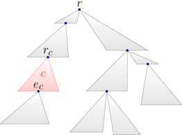
Figure 4: Decomposition into components. In this example, the tree is decomposed into four leaf components and six internal components. An internal component $c$ has a root vertex $r_{c}$ and an exit vertex $e_{c}$.

Lemma 9.

Let $\Gamma=\frac{12}{\epsilon}$. There is a polynomial time algorithm to compute a partition of the edges of the tree $T$ into a set $\mathcal{C}$ of components (see Fig. 4), such that all of the following properties are satisfied:

• Every component $c\in\mathcal{C}$ is a connected subgraph of $T$; the root vertex of the component $c$, denoted by $r_{c}$, is the vertex in $c$ that is closest to the depot.

• We say that a component $c\in\mathcal{C}$ is a leaf component if all descendants of $r_{c}$ in tree $T$ are in $c$, and is an internal component otherwise. A leaf component $c$ interacts with other components at vertex $r_{c}$ only. An internal component $c$ interacts with other components at two vertices only: at vertex $r_{c}$, and at another vertex, called the exit vertex of the component $c$, and denoted by $e_{c}$.

• Every component $c\in\mathcal{C}$ contains at most $2\Gamma\cdot k$ terminals. We say that a component is big if it contains at least $\Gamma\cdot k$ terminals. Each leaf component is big.

• If the number of components in $\mathcal{C}$ is strictly greater than one, then we have: (1) there exists a map from all components to big components, such that the image of a component is among its descendants (including itself), and each big component has at most three pre-images; and (2) the number of components in $\mathcal{C}$ is at most $3/\Gamma$ times the total demand in the tree $T$.

Remark 10.

The root and the exit vertices of components are a rough analog of portals used in approximation schemes for other problems: they are places where the dynamic program will gather and synthesize information about partial solutions before passing it on.

Compared with [BP19], the decomposition in Lemma 9 uses different parameters: the number of terminals inside a leaf component is $\Theta(k/\epsilon)$, whereas in [BP19] the number of terminals inside a leaf cluster is $\Theta(\epsilon\cdot k)$; the threshold demand to define big components is $\Theta(k/\epsilon)$, whereas in [BP19] the threshold demand to define small clusters is $\Theta(\epsilon^{2}\cdot k)$.

Definition 11 (subtours in components and subtour types).

Let $c$ be any component. A subtour in the component $c$ is a path that starts and ends at the root $r_{c}$ of the component, and such that every vertex on the path is in $c$. The type of a subtour is “passing” if $c$ is an internal component and the exit vertex $e_{c}$ belongs to that subtour; and is “ending” otherwise.

A passing subtour in $c$ is to be combined with a subtour at $e_{c}$. In a leaf component, there is no passing subtour.

Definition 12 (spine subtour).

For an internal component $c$, we define the spine subtour in the component $c$, denoted by $\mathrm{spine}_{c}$, to be the connection (in both directions) between the root vertex $r_{c}$ and the exit vertex $e_{c}$ of the component $c$, without visiting any terminal.

From the definition, a spine subtour in a component is also a passing subtour in that component.

Without loss of generality, we assume that any subtour in a component $c$ either visits at least one terminal in $c$ or is a spine subtour; that any tour traverses each edge of the tree at most twice (once in each direction); and that any tour contains at most one subtour in any component.

3 Solutions Inside Components

In this section, we prove Theorem 13, which is a main novelty in this paper.

Theorem 13.

Let $\alpha=\epsilon^{(\frac{1}{\epsilon}+1)}$. Consider the unit demand CVRP on the tree $T$ with bounded distances. There exist dummy terminals and a solution $\mathrm{OPT}_{1}$ visiting all of the real and the dummy terminals, such that all of the following holds:

1. For each component $c$, there are at most $\frac{2\Gamma}{\alpha}+1$ tours visiting terminals in $c$;

2. For each component $c$ and each tour $t$ visiting terminals in $c$, the number of the terminals in $c$ visited by $t$ is at least $\alpha\cdot k$;

3. We have $\mathrm{opt}_{1}\leq(1+\epsilon)\cdot\mathrm{opt}$.

3.1 Construction of $\mathrm{OPT}_{1}$

Definition 14 (large and small subtours).

We say that a subtour is large if its demand is at least $\alpha\cdot k$, and small otherwise.

The construction of $\mathrm{OPT}_{1}$, starting from an optimal solution $\mathrm{OPT}$, is in several steps.

Step 1: Detaching small subtours.

Prune each tour of $\mathrm{OPT}$ so that it only visits the terminals that do not belong to a small subtour in any component, and is minimal. In other words, if a tour $t$ in $\mathrm{OPT}$ contains a small ending subtour $t_{e}$ in a component $c$, then we remove $t_{e}$ from $t$; and if a tour $t$ in $\mathrm{OPT}$ contains a non-spine small passing subtour $t_{p}$ in a component $c$, then we remove $t_{p}$ from $t$, except for the spine subtour of $c$.

Let $A$ denote the set of the resulting tours. Note that each tour in $A$ is connected. The removed pieces of a non-spine small passing subtour $t_{p}$ may be disconnected from one another.

The parts of $\mathrm{OPT}$ that have been pruned consist of the set $\mathcal{E}$, each element being a small ending subtours in a component, and of the set $\mathcal{P}$, each element being a group of pieces in a component obtained from a non-spine small passing subtour by removing the corresponding spine subtour. The demand of a group of pieces in $\mathcal{P}$ is the number of terminals in all of the pieces in that group.

Step 2: Combining small subtours within components.

• For each component $c$, repeatedly concatenate subtours in $c$ from the set $\mathcal{E}$ so that in the end, all resulting subtours in $c$ from the set $\mathcal{E}$ have demands between $\alpha\cdot k$ and $2\alpha\cdot k$ except for at most one subtour.

• For each component $c$, repeatedly merge groups in $c$ from the set $\mathcal{P}$ so that in the end, all resulting groups in $c$ from the set $\mathcal{P}$ have demands between $\alpha\cdot k$ and $2\alpha\cdot k$ except for at most one group.

Let $\mathcal{E}^{\prime}$ and $\mathcal{P}^{\prime}$ denote the corresponding sets after the modifications for all components $c$. Let $B=\mathcal{E}^{\prime}\cup\mathcal{P}^{\prime}$. An element of $B$ is either a subtour or a group of pieces in a component $c$. For each component $c$, all elements of $B$ in the component $c$ have demands between $\alpha\cdot k$ and $2\alpha\cdot k$ except for at most two elements with smaller demands.

Step 3: Reassigning small subtours.

Construct a bipartite graph with vertex sets $A$ and $B$ and with edge set $E$. Let $a$ be any tour in $A$, and let $a_{0}$ denote the corresponding tour in $\mathrm{OPT}$. Let $b$ be any element in $B$. The set $E$ contains an edge between $a$ and $b$ if and only if the element $b$ contains terminals from $a_{0}$; the weight of the edge $(a,b)$ is the number of terminals in both $b$ and $a_{0}$. By Lemma 1 from [BP19], there exists an assignment $f:B\rightarrow A$ such that each element $b\in B$ is assigned to a tour $a\in A$ with $(a,b)\in E$ and that, for each tour $a\in A$, the demand of $a$ plus the overall demand of the elements $b\in B$ that are assigned to $a$ is at most the demand of the corresponding tour $a_{0}$ plus the maximum demand of any element in $B$.

Let $A_{1}$ denote the set of pseudo-tours induced by the assignment $f$. Each pseudo-tour in $A_{1}$ is the union of a tour $a\in A$ and the elements $b\in B$ that are assigned to $a$.

Step 4: Correcting tour capacities.

For each pseudo-tour $a_{1}$ in $A_{1}$, if the demand of $a_{1}$ exceeds $k$, we repeatedly remove an element $b\in B$ from $a_{1}$, until the demand of $a_{1}$ is at most $k$.

Let $A_{2}$ denote the resulting set of pseudo-tours. Every pseudo-tour in $A_{2}$ is a connected tour of demand at most $k$ (Lemma 15). Let $B^{*}\subseteq B$ denote the set of the removed elements $b\in B$. The elements in $B^{*}$ are represented by the small pieces in Fig. 2(a) (Fig. 2(a)).

Step 5: Creating additional tours.

We connect the elements of $B^{*}$ to the depot by creating additional tours as follows.

• Let $Q$ denote the union of the spine subtours for all internal components. $Q$ is represented by the green thick paths in Fig. 2(a). Let $X$ denote a multi-subgraph of $T$ that is the union of the elements in $B^{*}$ and the edges in $Q$. Observe that each element in $B^{*}$ is connected to the depot through edges in $Q$. Thus $X$ is connected, and induces a traveling salesman tour $t_{\mathrm{TSP}}$ visiting all terminals in $B^{*}$. Without loss of generality, we assume that, for any component $c$, if $t_{\mathrm{TSP}}$ visits terminals in $c$, then those terminals belong to a single subpath $p_{c}$ of $t_{\mathrm{TSP}}$, such that $p_{c}$ does not visit any terminal from other components.

• If the traveling salesman tour $t_{\mathrm{TSP}}$ is within the tour capacity, then let $A_{3}$ denote the set consisting of a single tour $t_{\mathrm{TSP}}$. Otherwise, we apply the iterated tour partitioning (ITP) algorithm [HR85] on $t_{\mathrm{TSP}}$: we partition $t_{\mathrm{TSP}}$ into segments with exactly $k$ terminals each, except possibly the last segments containing less than $k$ terminals. For each segment, we connect its endpoints to the depot so as to make a tour, see Fig. 2(b). Let $A_{3}$ denote the resulting set of tours.

Let $A_{4}=A_{2}\cup A_{3}$.

Step 6: Postprocessing.

For each component $c$, we rearrange the small subtours in $A_{4}$ as follows.

• For each tour $t$ in $A_{4}$ that contains a small subtour in $c$, letting $t_{c}$ denote this small subtour, if $t_{c}$ is an ending subtour, we remove $t_{c}$ from $t$; if $t_{c}$ is a passing subtour, we remove $t_{c}$ from $t$, except for the spine subtour in $c$. The total demand of all of the removed small subtours in $c$ is at most $k$ (Lemma 16).

• We create an additional tour $t^{*}_{c}$ from the depot that connects all of the removed small subtours in $c$. If the demand of $t^{*}_{c}$ is less than $\alpha\cdot k$, then we include dummy terminals at $r_{c}$ into the tour $t^{*}_{c}$ so that its demand is exactly $k$.

Let $A_{5}$ denote the resulting set of tours after removing small subtours from $A_{4}$. Let $A_{6}$ denote the set of newly created tours $\{t^{*}_{c}\}_{c\in\mathcal{C}}$.

Finally, let $\mathrm{OPT}_{1}=A_{5}\cup A_{6}$.

In Section 3.2, we show that $\mathrm{OPT}_{1}$ is a feasible solution to the unit demand tree CVRP; in Section 3.3, we prove the three properties of $\mathrm{OPT}_{1}$ in the claim of Theorem 13.

3.2 Feasibility of the Construction

Lemma 15.

Every pseudo-tour in $A_{2}$ is a connected tour of demand at most $k$.

Proof.

Let $a_{2}$ be any pseudo-tour in $A_{2}$. By the construction in Step 4, the demand of $a_{2}$ is at most $k$. It suffices to show that $a_{2}$ is a connected tour.

Observe that $a_{2}$ is the union of a tour $a\in A$ and some elements $b_{1},\dots,b_{q}$ from $B$, for $q\geq 0$. From the construction, any tour $a\in A$ is connected. Consider any $b_{i}$ for $i\in[1,q]$. Observe that $f(b_{i})=a$, so the edge $(a,b_{i})$ belongs to the bipartite graph $(A,B)$. If $b_{i}$ is a subtour at $r_{c}$ for some component $c$, then $r_{c}$ must belong to the tour $a$; and if $b_{i}$ is a group of pieces in some component $c$, then the spine subtour of $c$ must belong to the tour $a$. So the union of $a$ and $b_{i}$ is connected. Thus $a_{2}=a\cup b_{1}\cup\dots\cup b_{q}$ is a connected tour. ∎

Lemma 16.

In any component $c$, the total demand of all of the removed small subtours in $c$ at the beginning of Step 6 is at most $k$.

Proof.

Let $c$ be any component. The key is to show that the number of non-spine small subtours in $c$ that are contained in tours in $A_{4}$ is at most 4. Since $A_{4}=A_{2}\cup A_{3}$, we analyze the number of non-spine small subtours in $c$ that are contained in tours in $A_{2}$ and in $A_{3}$, respectively.

The tours in $A_{2}$ contain at most two non-spine small subtours in $c$, since at most two elements of $B$ in component $c$ have demands less than $\alpha\cdot k$.

We claim that the tours in $A_{3}$ contain at most two non-spine small subtours in $c$. If $A_{3}$ consists of a single tour $t_{\mathrm{TSP}}$, the claim follows trivially since any tour contains at most one subtour in $c$ from our assumption. Next, we consider the case when $A_{3}$ is generated by the ITP algorithm. From our assumption, if $t_{\mathrm{TSP}}$ visits terminals in $c$, then those terminals belong to a single subpath $p_{c}$ of $t_{\mathrm{TSP}}$, such that $p_{c}$ does not visit any terminal from other components. By applying the ITP algorithm on $t_{\mathrm{TSP}}$, we obtain a collection of segments. All segments that intersect $p_{c}$ visit exactly $k$ terminals in $c$, except for possibly the first and the last of those segments visiting less than $k$ terminals in $c$. Hence at most two non-spine small subtours in $c$ among the tours in $A_{3}$.

Therefore, the number of non-spine small subtours in $c$ in the solution $A_{4}$ is at most 4. Since each small subtour has demand at most $\alpha\cdot k$, the total demand of the removed small subtours is at most $4\cdot\alpha\cdot k<k$. ∎

3.3 Analysis of $\mathrm{OPT}_{1}$

Let $c\in\mathcal{C}$ be any component. From Lemma 9, $c$ contains at most $2\Gamma\cdot k$ real terminals. Each tour in $A_{5}$ visiting terminals in $c$ visits at least $\alpha\cdot k$ real terminals in $c$, so there are at most $\frac{2\Gamma}{\alpha}$ tours in $A_{5}$ visiting terminals in $c$. There is a single tour in $A_{6}$, the tour $t_{c}^{*}$, that visits terminals in $c$. Hence the first property of the claim. From the construction of $t_{c}^{*}$, the second property of the claim follows.

It remains to analyze the cost of $\mathrm{OPT}_{1}$. Compared with $\mathrm{OPT}$, the extra cost in $\mathrm{OPT}_{1}$ is due to Step 5 and Step 6 of the construction. This extra cost consists of the cost of the edges in $Q$ (Step 5), the cost in the ITP algorithm to connect the endpoints of all segments to the depot (Step 5), and the cost of the postprocessing (Step 6), which we bound in Corollaries 18, 19 and 20, respectively. Both Corollary 18 and Lemma 20 are based on Lemma 17.

Lemma 17.

We have $\displaystyle\sum_{\text{component $c$}}\mathrm{dist}(r_{c})\leq\frac{\epsilon}{8}\cdot\mathrm{opt}.$

Proof.

For any edge $e$ in $T$, let $u$ and $v$ denote the two endpoints of $e$ such that $u$ is the parent of $v$. Let $T_{e}$ denote the subtree of $T$ rooted at $v$. Let $n_{e}$ denote the number of terminals in $T_{e}$. From the lower bound in [HK98], we have

$$\mathrm{opt}\geq\sum_{e\in T}2\cdot w(e)\cdot\frac{n_{e}}{k}.$$

Since each big component contains at least $\Gamma\cdot k$ terminals, we have

$$n_{e}\geq\sum_{\text{big component }c\subseteq T_{e}}\Gamma\cdot k.$$

Thus

$$\mathrm{opt} \geq\sum_{e\in T}2\cdot w(e)\cdot\sum_{\text{big component }c\subseteq T_{e}}\Gamma$$

$$=\sum_{\text{big component }c}\Gamma\cdot\sum_{e\in T\text{ such that }c\subseteq T_{e}}2\cdot w(e)$$

$$=\sum_{\text{big component }c}\Gamma\cdot 2\cdot\mathrm{dist}(r_{c}).$$

From Lemma 9, there exists a map from all components to big components such that the image of a component is among its descendants (including itself) and each big component has at most three pre-images. Thus

$$3\cdot\sum_{\text{big component $c$}}\mathrm{dist}(r_{c})\geq\sum_{\text{component $c$}}\mathrm{dist}(r_{c}).$$

Therefore,

$$\mathrm{opt}\geq\frac{2\cdot\Gamma}{3}\cdot\sum_{\text{component $c$}}\mathrm{dist}(r_{c}).$$

The claim follows since $\Gamma=\frac{12}{\epsilon}$. ∎

Corollary 18.

We have $\mathrm{cost}(Q)\leq\frac{\epsilon}{4}\cdot\mathrm{opt}$.

Proof.

Observe that every edge in $Q$ belongs to the connection (in both directions) between the depot and the root of some component $c$. By Lemma 17, we have

$$\mathrm{cost}(Q)\leq 2\cdot\sum_{\text{component $c$}}\mathrm{dist}(r_{c})\leq\frac{\epsilon}{4}\cdot\mathrm{opt}.$$

Lemma 19.

Let $\Delta_{1}$ denote the cost in the ITP algorithm to connect the endpoints of all segments to the depot in Step 5. We have $\Delta_{1}\leq\frac{\epsilon}{4}\cdot\mathrm{opt}$.

Proof.

Let $n^{\prime}$ denote the number of terminals in the tree $T$. First, we show that the number of terminals on $t_{\mathrm{TSP}}$ is at most $4\alpha\cdot n^{\prime}$. Observe that the number of terminals on $t_{\mathrm{TSP}}$ is the overall removed demand in Step 4. Consider any pseudo-tour $a_{1}\in A_{1}$ whose demand exceeds $k$. Let $a_{0}$ denote the corresponding tour in $\mathrm{OPT}$. By the construction, the demand of $a_{1}$ is at most the demand of $a_{0}$ plus the maximum demand of any element in $B$. Since the demand of $a_{0}$ is at most $k$ and the demand of any element in $B$ is at most $2\alpha\cdot k$, the demand of $a_{1}$ is at most $k+2\alpha\cdot k$. Let $a_{2}$ denote the corresponding tour after the correction of capacity in Step 4. Since any element in $B$ has demand at most $2\alpha\cdot k$, the demand of $a_{2}$ is at least $k-2\alpha\cdot k$. So the total removed demand from $a_{1}$ in Step 4 is at most $4\alpha\cdot k$. There are at most $\frac{n^{\prime}}{k}$ pseudo-tours $a_{1}\in A_{1}$ whose demands exceed $k$. Summing over all those pseudo-tours, the overall removed demand in Step 4 is at most $\frac{n^{\prime}}{k}\cdot 4\alpha\cdot k=4\alpha\cdot n^{\prime}$. Hence the number of terminals on $t_{\mathrm{TSP}}$ is at most $4\alpha\cdot n^{\prime}$.

If $4\alpha\cdot n^{\prime}\leq k$, then $t_{\mathrm{TSP}}$ is within the tour capacity, so the ITP algorithm is not applied and $\Delta_{1}=0$. It remains to consider the case in which $4\alpha\cdot n^{\prime}>k$. By the construction in the ITP algorithm, every segment visits exactly $k$ terminals except possibly the last segment. Thus the number $\ell_{\text{ITP}}$ of resulting tours in the ITP algorithm is

$$\ell_{\text{IPT}}\leq\frac{4\alpha\cdot n^{\prime}}{k}+1.$$ (1)

Since $4\alpha\cdot n^{\prime}>k$, we have $\ell_{\text{IPT}}<\frac{8\alpha\cdot n^{\prime}}{k}$. Since $\Delta_{1}\leq\ell_{\text{ITP}}\cdot 2\cdot D_{\max}$ and using Definition 3 and the definition of $\alpha$ in the claim of Theorem 13, we have

$$\Delta_{1}<\frac{8\alpha\cdot n^{\prime}}{k}\cdot 2\cdot\left(\frac{1}{\epsilon}\right)^{\frac{1}{\epsilon}-1}\cdot D_{\min}<\frac{\epsilon}{2}\cdot\frac{n^{\prime}}{k}\cdot D_{\min}.$$

On the other hand, the solution $\mathrm{OPT}$ consists of at least $\frac{n^{\prime}}{k}$ tours, so $\mathrm{opt}\geq\frac{2n^{\prime}}{k}\cdot D_{\min}.$ Therefore, $\Delta_{1}\leq\frac{\epsilon}{4}\cdot\mathrm{opt}$. ∎

Lemma 20.

Let $\Delta_{2}$ denote the cost of the postprocessing (Step 6). Then $\Delta_{2}\leq\frac{\epsilon}{2}\cdot\mathrm{opt}$.

Proof.

For each leaf component $c$, the cost to connect the small subtours in $c$ to the depot in Step 6 is at most $2\cdot\mathrm{dist}(r_{c})$; and for each internal component $c$, the cost to connect the small subtours in $c$ to the depot is at most $2\cdot\mathrm{dist}(r_{c})+\mathrm{cost}(\mathrm{spine}_{c})$. Summing over all components, we have

$$\Delta_{2}\leq\sum_{\text{component }c}2\cdot\mathrm{dist}(r_{c})+\sum_{\text{internal component }c}\mathrm{cost}(\mathrm{spine}_{c}).$$

By Lemma 17, we have

$$\sum_{\text{component }c}2\cdot\mathrm{dist}(r_{c})\leq\frac{\epsilon}{4}\cdot\mathrm{opt}$$

and

$$\sum_{\text{internal component }c}\mathrm{cost}(\mathrm{spine}_{c})=\mathrm{cost}(Q)\leq\frac{\epsilon}{4}\cdot\mathrm{opt}.$$

Thus $\Delta_{2}\leq\frac{\epsilon}{2}\cdot\mathrm{opt}$. ∎

From Corollaries 18, 19 and 20, we have $\mathrm{opt}_{1}\leq\mathrm{opt}+\mathrm{cost}(Q)+\Delta_{1}+\Delta_{2}\leq(1+\epsilon)\cdot\mathrm{opt}$. This completes the proof for Theorem 13.

4 Height Reduction

In this section, we transform the tree $T$ into a tree $\hat{T}$ so that $\hat{T}$ has $O_{\epsilon}(1)$ levels of components, see Fig. 1. We assume that the tree $T$ has bounded distances. To begin with, we partition the components according to the distances from their roots to the depot.

Lemma 21.

Let $\tilde{D}=\alpha\cdot\epsilon\cdot D_{\min}$. Let $H_{\epsilon}=(\frac{1}{\epsilon})^{\frac{2}{\epsilon}+1}$. For each $i\in[1,H_{\epsilon}]$, let $\mathcal{C}_{i}\subseteq\mathcal{C}$ denote the set of components $c\in\mathcal{C}$ such that $\mathrm{dist}(r_{c})\in\left[(i-1)\cdot\tilde{D},i\cdot\tilde{D}\right)$. Then any component $c\in\mathcal{C}$ belongs to a set $\mathcal{C}_{i}$ for some $i\in[1,H_{\epsilon}]$.

Proof.

Let $c\in\mathcal{C}$ be any component. We have

$$\mathrm{dist}(r_{c})\leq D_{\max}<\left(\frac{1}{\epsilon}\right)^{\frac{1}{\epsilon}-1}\cdot D_{\min}=H_{\epsilon}\cdot\tilde{D},$$

where the second inequality follows from Definition 3, and the equality follows from the definition of $\alpha$ in Theorem 13 and the definitions of $\tilde{D}$ and $H_{\epsilon}$. Thus there exists $i\in[1,H_{\epsilon}]$ such that $c\in\mathcal{C}_{i}$. ∎

Definition 22 (maximally connected sets and critical vertices).

We say that a set of components $\tilde{\mathcal{C}}\subseteq\mathcal{C}_{i}$ is maximally connected if the components in $\tilde{\mathcal{C}}$ are connected to each other and $\tilde{\mathcal{C}}$ is maximal within $\mathcal{C}_{i}$. For a maximally connected set of components $\tilde{\mathcal{C}}\subseteq\mathcal{C}_{i}$, we define the critical vertex of $\tilde{\mathcal{C}}$ to be the root vertex of the component $c\in\tilde{\mathcal{C}}$ that is closest to the depot.

Fig. 1 (Fig. 1) is an example with three levels of components: $\mathcal{C}_{1}$, $\mathcal{C}_{2}$, and $\mathcal{C}_{3}$, indicated by different colors. There are four maximally connected sets of components. The critical vertices are represented by rectangular nodes.

Algorithm 1 Construction of the tree $\hat{T}$ (see Fig. 1).

1:for each $i\in[1,H_{\epsilon}]$ do

2:     for each maximally connected set of components $\tilde{\mathcal{C}}\subseteq\mathcal{C}_{i}$ do

3:         $z\leftarrow$ critical vertex of $\tilde{\mathcal{C}}$

4:         for each component $c\in\tilde{\mathcal{C}}$ do

5:              $\delta\leftarrow r_{c}$-to-$z$ distance in $T$

6:              Split the tree $T$ at the root vertex $r_{c}$ of the component $c$ $\triangleright$ vertex $r_{c}$ is duplicated

7:              Add an edge between the root of the component $c$ and $z$ with weight $\delta$               

8:$\hat{T}\leftarrow$the resulting tree

Let $\hat{T}$ be the tree constructed in Algorithm 1. We observe that Algorithm 1 is in polynomial time, and 6 follows from the construction. We show in Theorem 23 that the optimal cost for $\hat{T}$ is increased by an $O(\epsilon)$ fraction compared with the optimal cost for $T$.

Theorem 23.

Consider the unit demand CVRP on the tree $\hat{T}$. There exist dummy terminals and a solution $\mathrm{OPT}_{2}$ visiting all of the real and the dummy terminals, such that all of the following holds:

1. For each component $c$, there are at most $\frac{2\Gamma}{\alpha}+1$ tours visiting terminals in $c$;

2. For each component $c$ and each tour $t$ visiting terminals in $c$, the number of the terminals in $c$ visited by $t$ is at least $\alpha\cdot k$;

3. We have $\mathrm{opt}_{2}<(1+3\epsilon)\cdot\mathrm{opt}$, where $\mathrm{opt}$ denotes the optimal cost for the unit demand CVRP on the tree $T$.

In the rest of the section, we prove Theorem 23.

4.1 Construction of $\mathrm{OPT}_{2}$

Consider any tour $t$ in $\mathrm{OPT}_{1}$. Let $U$ denote the set of terminals visited by $t$. We define the tour $\hat{t}$ as the minimal tour in the tree $\hat{T}$ that spans all terminals in $U$, see Fig. 1. Let $\mathrm{OPT}_{2}$ denote the set of the resulting tours on the tree $\hat{T}$ constructed from every tour $t$ in $\mathrm{OPT}_{1}$. Then $\mathrm{OPT}_{2}$ is a feasible solution to the unit demand CVRP on $\hat{T}$.

4.2 Analysis of $\mathrm{OPT}_{2}$

The first two properties in Theorem 23 follow from the construction and Theorem 13.

In the rest of the section, we analyze the cost of $\mathrm{OPT}_{2}$.

Lemma 24.

Let $t$ denote any tour in $\mathrm{OPT}_{1}$. Let $\hat{t}$ denote the corresponding tour in $\mathrm{OPT}_{2}$. Then $\mathrm{cost}(\hat{t})\leq(1+\epsilon)\cdot\mathrm{cost}(t)$.

Proof.

We follow the notation on $U$ from Section 4.1. Let $\mathcal{C}(U)$ denote the set of components $c\in\mathcal{C}$ that contains a (possibly spine) subtour of $\hat{t}$. Observe that the cost of $\hat{t}$ consists of the following two parts:

1. for each component $c\in\mathcal{C}(U)$, the cost of the subtour in $c$ from the tour $t$; we charge that cost to the subtour in $t$;

2. for each component $c\in\mathcal{C}(U)$, the cost of the edge $(r_{c},z)$, where $z$ denotes the father vertex of $r_{c}$ in $\hat{T}$. Note that $z$ is a critical vertex on $\hat{t}$. We analyze that cost over all components $c\in\mathcal{C}(U)$ as follows.

Let $Z\subseteq V$ denote the set of critical vertices $z\in V$ on $\hat{t}$. For any critical vertex $z\in Z$, let $Y(z)$ denote the set of edges $(z,v)$ in the tree $\hat{T}$ such that $v$ is a child of $z$ and that the edge $(z,v)$ belongs to the tour $\hat{t}$. The overall cost of the second part is the total cost of the edges in $Y(z)$ for all $z\in Z$.

Fix a critical vertex $z\in Z$. Let $(z,v_{1})$ denote the edge in $Y(z)$ such that $\mathrm{dist}(v_{1})$ is minimized, breaking ties arbitrarily. From the minimality of $\mathrm{dist}(v_{1})$, the $z$-to-$v_{1}$ path in $T$ does not go through any component in $\mathcal{C}(U)$. From the construction, the cost of the edge $(z,v_{1})$ in $\hat{T}$ equals the cost of the $z$-to-$v_{1}$ path in $T$. It is easy to see that the $z$-to-$v_{1}$ path in $T$ belongs to the tour $t$. Indeed, tour $\hat{t}$ traverses the edge $(z,v_{1})$ on its way to visit some terminals of $U$ in the subtree rooted at $v_{1}$. In order to visit the corresponding terminals in $T$, tour $t$ must traverse the $z$-to-$v_{1}$ path. We charge the cost of the edge $(z,v_{1})$ in $\hat{T}$ to the $z$-to-$v_{1}$ path in $T$. Next, we analyze the cost due to the other edges in $Y(z)$. Consider one such edge $(z,v)$. From the construction, there exists $i\in[1,H_{\epsilon}]$, such that both $\mathrm{dist}(z)$ and $\mathrm{dist}(v)$ belong to $\left[(i-1)\cdot\tilde{D},i\cdot\tilde{D}\right)$. Thus the cost of the $z$-to-$v$ path in $T$ equals $\mathrm{dist}(v)-\mathrm{dist}(z)<\tilde{D}$, so the extra cost in $\hat{t}$ due to the edge $(z,v)$ is at most $2\cdot\tilde{D}$ (for both directions). Therefore, the extra cost in $\hat{t}$ due to those $|Y(z)|-1$ edges in $Y(z)$ is at most $2\cdot\tilde{D}\cdot(|Y(z)|-1)$.

Summing over all vertices $z\in Z$, and observing that all charges are to disjoint parts of $t$, we have

$$\mathrm{cost}(\hat{t})\leq\mathrm{cost}(t)+2\cdot\tilde{D}\cdot\sum_{z\in Z}(|Y(z)|-1).$$ (2)

It remains to bound $\sum_{z\in Z}(|Y(z)|-1)$. The analysis uses the following basic fact in trees.

Fact 25.

Let $H$ be a tree with $L$ leaves. For each vertex $u$ in $H$, let $m(u)$ denote the number of children of $u$ in $H$. Then

$$\sum_{u\in H}(m(u)-1)\leq L-1.$$

We construct a tree $H$ as follows. Starting from the tree spanning $U$ in $\hat{T}$, we contract vertices in each component $c\in\mathcal{C}(U)$ into a single vertex; let $H$ denote the resulting tree. It is easy to see that each leaf in $H$ corresponds to a component $c\in\mathcal{C}(U)$ that contains at least one terminal in $U$ (using the definition of $\mathcal{C}(U)$ and the fact that any descending component of $c$ do not belong to $\mathcal{C}(U)$). From the second property of Theorem 23 (which follows from Theorem 13), terminals in $U$ belong to at most $1/\alpha$ components. Thus, by 25 we have

$$\sum_{z\in Z}(|Y(z)|-1)\leq(1/\alpha)-1.$$

Combined with Eq. 2, we have

$$\mathrm{cost}(\hat{t})-\mathrm{cost}(t)<2\cdot\tilde{D}\cdot(1/\alpha)=2\cdot\alpha\cdot\epsilon\cdot D_{\min}\cdot(1/\alpha)=2\epsilon\cdot D_{\min},$$

using the definition of $\tilde{D}$ in Lemma 21. Since $\mathrm{cost}(t)\geq 2\cdot D_{\min}$, the claim follows. ∎

Applying Lemma 24 on each tour $t$ in $\mathrm{OPT}_{1}$ and summing, we have $\mathrm{opt}_{2}\leq(1+\epsilon)\cdot\mathrm{opt}_{1}$. By Theorem 13, $\mathrm{opt}_{1}\leq(1+\epsilon)\cdot\mathrm{opt}$, thus $\mathrm{opt}_{2}\leq(1+3\epsilon)\cdot\mathrm{opt}$. This completes the proof of Theorem 23.

5 Adaptive Rounding on the Subtour Demands

In this section, we prove Theorem 26. We use the adaptive rounding to show that, in a near-optimal solution, the demands of the subtours at any critical vertex are from a set of $O_{\epsilon}(1)$ values. This property enables us to later guess those values in polynomial time by a dynamic program (see Section 6).

Theorem 26.

Let $\beta=\frac{1}{4}\cdot\epsilon^{(\frac{4}{\epsilon}+1)}$. Consider the unit demand CVRP on the tree $\hat{T}$. There exist dummy terminals and a solution $\mathrm{OPT}_{3}$ visiting all of the real and the dummy terminals, such that all of the following holds:

1. For each component $c$, there are at most $\frac{2\Gamma}{\alpha}+1$ tours visiting terminals in $c$;

2. For each critical vertex $z$, there exist $\frac{1}{\beta}$ integer values in $[\alpha\cdot k,k]$ such that the demands of the subtours at the children of $z$ are among these values;

3. We have $\mathrm{opt}_{3}<(1+4\epsilon)\cdot\mathrm{opt}$, where $\mathrm{opt}$ denotes the optimal cost for the unit demand CVRP on the tree $T$.

5.1 Construction of $\mathrm{OPT}_{3}$

We construct the solution $\mathrm{OPT}_{3}$ by modifying the solution $\mathrm{OPT}_{2}$.

Let $I\subseteq V$ denote the set of vertices $v\in V$ that is either the root of a component or a critical vertex. Consider any vertex $v\in I$ in the bottom up order. Let $\mathrm{OPT}_{2}(v)$ denote the set of subtours at $v$ in $\mathrm{OPT}_{2}$. We construct a set $A(v)$ of subtours at $v$ satisfying the following invariants:

• the subtours in $A(v)$ have a one-to-one correspondence with the subtours in $\mathrm{OPT}_{2}(v)$; and

• the demand of each subtour of $A(v)$ is at most that of the corresponding subtour in $\mathrm{OPT}_{2}(v)$.

The construction of $A(v)$ is according to one of the following three cases on $v$.

Case 1: $v$ is the root vertex $r_{c}$ of a leaf component $c$ in $\hat{T}$.

Let $A(v)=\mathrm{OPT}_{2}(v)$.

Case 2: $v$ is the root vertex $r_{c}$ of an internal component $c$ in $\hat{T}$.

For each subtour $a\in\mathrm{OPT}_{2}(v)$, if $a$ contains a subtour at the exit vertex $e_{c}$ of component $c$, letting $t$ denote this subtour and $t^{\prime}$ denote the subtour in $A(e_{c})$ corresponding to $t$, we replace the subtour $t$ in $a$ by the subtour $t^{\prime}$. Let $A(v)$ be the resulting set of subtours at $v$.

Case 3: $v$ is a critical vertex in $\hat{T}$.

We apply the technique of the adaptive rounding, previously used by Jayaprakash and Salavatipour [JS22] in their design of a QPTAS the tree CVRP. The idea is to round up the demands of the subtours at the children of $v$ so that the resulting demands are among $\frac{1}{\beta}$ values.

Let $r_{1},\dots,r_{m}$ be the children of $v$ in $\hat{T}$. For each subtour $a\in\mathrm{OPT}_{2}(v)$ and for each $i\in[1,m]$, if $a$ contains a subtour at $r_{i}$, letting $t$ denote this subtour and $t^{\prime}$ denote the subtour in $A(r_{i})$ corresponding to $t$, we replace $t$ in $a$ by $t^{\prime}$. Let $A_{1}(v)$ denote the resulting set of subtours at $v$.

Let $W_{v}$ denote the set of the subtours at the children of $v$ in $A_{1}(v)$, i.e., $W_{v}=A(r_{1})\cup\dots\cup A(r_{m})$. If $|W_{v}|\leq\frac{1}{\beta}$, let $A(v)=A_{1}(v)$. In the following, we consider the non-trivial case when $|W_{v}|>\frac{1}{\beta}$. We sort the subtours in $W_{v}$ in non-decreasing order of their demands, and partition these subtours into $\frac{1}{\beta}$ groups of equal cardinality. We round the demands of the subtours in each group to the maximum demand in that group. The demand of a subtour is increased to the rounded value by adding dummy terminals at the children of $v$. We rearrange the subtours in $W_{v}$ as follows.

• Each subtour $t\in W_{v}$ in the last group is discarded, i.e., detached from the subtour in $A_{1}(v)$ to which it belongs.

• Each subtour $t\in W_{v}$ in other groups is associated in a one-to-one manner to a subtour $t^{\prime}\in W_{v}$ in the next group. Letting $a$ (resp. $a^{\prime}$) denote the subtour in $A_{1}(v)$ to which $t$ (resp. $t^{\prime}$) belongs, we detach $t$ from $a$ and reattach $t$ to $a^{\prime}$.

Let $A(v)$ be the set of the resulting subtours at $v$ after the rearrangement for all $t\in W_{v}$.

For each subtour $t$ that is discarded in the construction, we complete $t$ into a separate tour by adding the connection (in both directions) to the depot. Let $B$ denote the set of these newly created tours. Let $\mathrm{OPT}_{3}=A(r)\cup B$.

It is easy to see that $\mathrm{OPT}_{3}$ is a feasible solution to the unit demand CVRP, i.e., each tour in $\mathrm{OPT}_{3}$ is connected and visits at most $k$ terminals, and each terminal is covered by some tour in $\mathrm{OPT}_{3}$.

5.2 Analysis of $\mathrm{OPT}_{3}$

From the construction, in any component $c\in\mathcal{C}$, the non-spine subtours in $\mathrm{OPT}_{3}$ are the same as those in $\mathrm{OPT}_{2}$. From Theorem 23, we obtain the first property in Theorem 26, and in addition, each subtour at a child of a critical vertex in $\mathrm{OPT}_{2}$ has demand at least $\alpha\cdot k$. The second property of the claim follows from the construction of $\mathrm{OPT}_{3}$.

It remains to analyze the cost of $\mathrm{OPT}_{3}$. Let $\Delta=\mathrm{opt}_{3}-\mathrm{opt}_{2}$. Observe that $\Delta$ is due to adding connections to the depot to create the tours in the set $B$.

Fix any $i\in[1,H_{\epsilon}]$. Let $Z\subseteq V$ denote the set of vertices $v\in V$ such that $v$ is the critical vertex of a maximally connected component $\tilde{\mathcal{C}}\subseteq\mathcal{C}_{i}$. For any $v\in Z$, we analyze the number of discarded subtours in the set $W_{v}$ defined in Section 5.1. If $|W_{v}|\leq\frac{1}{\beta}$, there is no discarded subtour in $W_{v}$; if $|W_{v}|>\frac{1}{\beta}$, the number of discarded subtours in $W_{v}$ is $\lceil\beta\cdot|W_{v}|\rceil<\beta\cdot|W_{v}|+1<2\beta\cdot|W_{v}|$. Let $W$ denote the disjoint union of $W_{v}$ for all vertices $v\in Z$. Thus $W$ contains at most $2\beta\cdot|W|$ discarded subtours. Let $\Delta_{i}$ denote the cost to connect the discarded subtours in $W$ to the depot. We have

$$\Delta_{i}\leq 2\beta\cdot|W|\cdot 2\cdot D_{\max}<\frac{1}{2}\cdot\epsilon^{(\frac{4}{\epsilon}+1)}\cdot|W|\cdot 2\cdot\left(\frac{1}{\epsilon}\right)^{\frac{1}{\epsilon}-1}\cdot D_{\min}=\frac{\epsilon}{H_{\epsilon}}\cdot\alpha\cdot|W|\cdot D_{\min},$$ (3)

where the second inequality follows from the definition of $\beta$ (Theorem 26) and Definition 3, and the equality follows from the definitions of $\alpha$ (Theorem 13) and of $H_{\epsilon}$ (Lemma 21). From the second property of the claim, each subtour in $W$ has demand at least $\alpha\cdot k$, so there are at least $\alpha\cdot|W|$ tours in $\mathrm{OPT}_{3}$. Any tour in $\mathrm{OPT}_{3}$ has cost at least $2\cdot D_{\min}$, so we have

$$\mathrm{opt}_{3}\geq 2\cdot\alpha\cdot|W|\cdot D_{\min}.$$ (4)

From Eqs. 3 and 4, we have

$$\Delta_{i}<\frac{\epsilon}{2\cdot H_{\epsilon}}\cdot\mathrm{opt}_{3}.$$

Summing over all integers $i\in[1,H_{\epsilon}]$, we have $\Delta=\sum_{i}\Delta_{i}\leq\frac{\epsilon}{2}\cdot\mathrm{opt}_{3}$. Thus

$$\mathrm{opt}_{3}\leq\frac{2}{2-\epsilon}\cdot\mathrm{opt}_{2}.$$

By Theorem 23, $\mathrm{opt}_{2}\leq(1+3\epsilon)\cdot\mathrm{opt}$. Therefore, $\mathrm{opt}_{3}\leq(1+4\epsilon)\cdot\mathrm{opt}$. This completes the proof of Theorem 26.

6 Dynamic Programming

In this section, we show Theorem 7. In our dynamic program, we consider all feasible solutions on the tree $\hat{T}$ satisfying the properties of $\mathrm{OPT}_{3}$ in Theorem 26, and we output the solution with minimum cost. The first property of Theorem 26 is used in Section 6.1 in the computation of solutions inside components, and the second property of Theorem 26 is used in Section 6.2 in the computation of solutions in the subtrees rooted at critical vertices. These two properties ensure the polynomial running time of the dynamic program. The cost of the output solution is at most the cost of $\mathrm{OPT}_{3}$, which is at most $(1+4\epsilon)$ times the optimal cost on the tree $T$ by the third property of Theorem 26.

6.1 Local Configurations

In this subsection, we compute values at local configurations (Definition 27), which are solutions restricted locally to a component. We require that the terminals in any component are visited by at most $\frac{2\Gamma}{\alpha}+1$ tours, using the first property in Theorem 26. Thus the number of local configurations is polynomially bounded.

Definition 27 (local configurations).

Let $c\in\mathcal{C}$ be any component. A local configuration $(v,A)$ is defined by a vertex $v\in c$ and a list $A$ of $\ell(A)$ pairs $(s_{1},b_{1}),(s_{2},b_{2}),\ldots,(s_{\ell(A)},b_{\ell(A)})$ such that

• $\ell(A)\leq\frac{2\Gamma}{\alpha}+1$;

• for each $i\in[1,\ell(A)]$, $s_{i}$ is an integer in $[0,k]$ and $b_{i}\in\{``\hbox{passing}",``\hbox{ending}"\}$.

When $v=r_{c}$, the local configuration $(r_{c},A)$ is also called a local configuration in the component $c$.

The value of a local configuration $(v,A)$, denoted by $f(v,A)$, equals the minimum cost of a collection of $\ell(A)$ subtours in the subtree of $c$ rooted at $v$, each subtour starting and ending at $v$, that together visit all of the terminals of the subtree of $c$ rooted at $v$, where the $i$-th subtour visits $s_{i}$ terminals and that $b_{i}=\text{``passing''}$ if and only if the $i$-th subtour visits $e_{c}$.

Let $v$ be any vertex in $c$. We compute the function $f(v,\cdot)$ according to one of the three cases.

Case 1: $v$ is the exit vertex $e_{c}$ of the component $c$.

For each $\ell\in[0,2\Gamma/\alpha+1]$, letting $A$ denote the list consisting uniquely of $\ell$ identical pairs of $(0,\text{``passing''})$, we set $f(v,A)=0$; for the remaining lists $A$, we set $f(v,A)=+\infty$.

Case 2: $v$ is a leaf vertex of the tree $\hat{T}$.

From Section 2 and the construction of $\hat{T}$, the leaf vertices in $\hat{T}$ are the same as the terminals in $\hat{T}$. Thus $v$ is a terminal in $\hat{T}$. For the list $A$ consisting of a single pair of $(1,\text{``ending''})$, we set $f(v,A)=0$; for the remaining lists $A$, we set $f(v,A)=+\infty$.

Case 3: $v$ is a non-leaf vertex of the tree $\hat{T}$ and $v\neq e_{c}$.

Let $v_{1}$ and $v_{2}$ be the two children of $v$. We say that the local configurations $(v_{1},A_{1})$, $(v_{2},A_{2})$, and $(v,A)$ are compatible if there is a partition $\mathcal{P}$ of $A_{1}\cup A_{2}$ into parts, each part consisting of one or two pairs, and a one-to-one correspondence between every part in $\mathcal{P}$ and every pair in $A$ such that:

• a part in $\mathcal{P}$ consisting of one pair $(s^{(1)},b^{(1)})$ corresponds to a pair $(s,b)$ in $A$ if and only if $s^{(1)}=s$ and $b^{(1)}=b$;

• a part in $\mathcal{P}$ consisting of two pairs $(s^{(1)},b^{(1)})$ and $(s^{(2)},b^{(2)})$ corresponds to a pair $(s,b)$ in $A$ if and only if $s=s^{(1)}+s^{(2)}$ and

  $$b=\begin{cases}\text{``passing'',}&\text{if $b^{(1)}$ is ``passing'' or $b^{(2)}$ is ``passing''},\\ \text{``ending'',}&\text{if $b^{(1)}$ is ``ending'' and $b^{(2)}$ is ``ending''.}\\ \end{cases}$$

We set

$$f(v,A)=\min\big{\{}f(v_{1},A_{1})+f(v_{2},A_{2})+2\cdot\ell(A_{1})\cdot w(v,v_{1})+2\cdot\ell(A_{2})\cdot w(v,v_{2})\big{\}},$$

where the minimum is taken over all local configurations $(v_{1},A_{1})$ and $(v_{2},A_{2})$ that are compatible with $(v,A)$.

The algorithm is very simple. See Algorithm 2.

Algorithm 2 Computation for local configurations in a component $c$.

1:for each vertex $v\in c$ and each list $A$ do

2:     $f(v,A)=+\infty$.

3:for each leaf vertex $v$ of $c$ do$\triangleright$ Cases 1 & 2

4:     Initialize $f(v,\cdot)$

5:for each non-leaf vertex $v$ of $c$ in the bottom-up order  do$\triangleright$ Case 3

6:     Let $v_{1}$ and $v_{2}$ denote the two children of $v$

7:     for each local configurations $(v_{1},A_{1})$, $(v_{2},A_{2})$, and $(v,A)$ do

8:         if $(v_{1},A_{1})$, $(v_{2},A_{2})$, and $(v,A)$ are compatible then

9:              $f(v,A)\leftarrow\min(f(v,A),f(v_{1},A_{1})+f(v_{2},A_{2})+2\cdot\ell(A_{1})\cdot w(v,v_{1})+2\cdot\ell(A_{2})\cdot w(v,v_{2}))$               

10:return $f(r_{c},\cdot)$

Running time.

For each vertex $v$, since $\ell(A)=O_{\epsilon}(1)$, the number of local configurations $(v,A)$ is $n^{O_{\epsilon}(1)}$. For fixed $(v_{1},A_{1}),(v_{2},A_{2})$, and $(v,A)$, there are $O_{\epsilon}(1)$ partitions of $A_{1}\cup A_{2}$ into parts, so checking compatibility takes time $O_{\epsilon}(1)$. Thus the running time to compute the values at local configurations in a component $c$ is $n^{O_{\epsilon}(1)}$. Since the number of components $c\in\mathcal{C}$ is at most $n$, the overall running time to compute the local configurations in all components $c\in\mathcal{C}$ is $n^{O_{\epsilon}(1)}$.

6.2 Subtree Configurations

In this subsection, we combine local configurations in the bottom up order to obtain subtree configurations (Definition 28), which are solutions restricted to subtrees of $\hat{T}$. The number of subtree configurations is polynomially bounded. When the subtree equals the tree $\hat{T}$, we obtain the entire solution to the CVRP.

Definition 28.

A subtree configuration $(v,A)$ is defined by a vertex $v$ and a list $A$ consisting of $\ell(A)$ pairs $(\tilde{s}_{1},n_{1})$, $(\tilde{s}_{2},n_{2}),\ldots,(\tilde{s}_{\ell},n_{\ell(A)})$ such that

• $v$ belongs to the set $I$ (defined in Section 5.1); in other words, $v$ is either the root of a component or a critical vertex;

• $\ell(A)\leq\left(\frac{1}{\beta}\right)^{\frac{1}{\alpha}}+\frac{2\Gamma}{\alpha}+1$ if $v$ is the root of a component, and $\ell(A)\leq\left(\frac{1}{\beta}\right)^{\frac{1}{\alpha}}$ if $v$ is a critical vertex;

• for each $i\in[1,\ell(A)]$, $\tilde{s}_{i}$ is an integer in $[0,k]$ and $n_{i}$ is an integer in $[0,n]$.

The value of the subtree configuration $(v,A)$, denoted by $g(v,A)$, is the minimum cost of a collection of $\ell(A)$ subtours in the subtree of $\hat{T}$ rooted at $v$, each subtour starting and ending at $v$, that together visit all of the real terminals of the subtree rooted at $v$, such that $n_{i}$ subtours visit $\tilde{s}_{i}$ (real and dummy) terminals each.

To compute the values of subtree configurations, we consider the vertices $v\in I$ in the bottom up order. See Fig. 3 (Fig. 3). For each vertex $v\in I$ that is the root of a component, we compute the values $g(v,\cdot)$ using the algorithm in Section 6.2.1; and for each vertex $v\in I$ that is a critical vertex, we compute the values $g(v,\cdot)$ using the algorithm in Section 6.2.2.

6.2.1 Subtree Configurations at the Root of a Component

In this subsection, we compute the values of the subtree configurations at the root $r_{c}$ of a component $c$. From Section 6.1, we have already computed the values of the local configurations in the component $c$.

If $c$ is a leaf component, the local configurations in $c$ induce the subtree configurations at $r_{c}$, in which $\tilde{s}_{i}=s_{i}$ and $n_{i}=1$ for all $i$. Thus we obtain the values of the subtree configurations at $r_{c}$.

In the following, we consider the case when $c$ is an internal component. We observe that the exit vertex $e_{c}$ of the component $c$ is a critical vertex. Thus the values of subtree configurations at $e_{c}$ have already been computed using Algorithm 4 in Section 6.2.2 according to the bottom up order of the computation. To compute the value of a subtree configuration at $r_{c}$, we combine a subtree configuration at $e_{c}$ and a local configuration in $c$, in the following way.

Let $A_{e}=((\tilde{s}_{1},n_{1}),(\tilde{s}_{2},n_{2}),\ldots,(\tilde{s}_{\ell_{e}},n_{\ell_{e}}))$ be the list from a subtree configuration $(e_{c},A_{e})$. Let $A_{c}=((s_{1},b_{1}),(s_{2},b_{2}),\dots,(s_{\ell_{c}},b_{\ell_{c}}))$ be the list from a local configuration $(r_{c},A_{c})$. To each $i\in[1,\ell_{c}]$ such that $b_{i}$ is “passing”, we associate $s_{i}$ with $\tilde{s}_{j}$ for some $j\in[1,\ell_{e}]$ with the constraints that $s_{i}+\tilde{s}_{j}\leq k$ (to guarantee that when we combine the two subtours, the result respects the capacity constraint) and that for each $j\in[1,\ell_{e}]$ at most $n_{j}$ elements are associated to $\tilde{s}_{j}$ (because in the subtree rooted at $e_{c}$ we only have $n_{j}$ subtours of demand $\tilde{s}_{j}$ at our disposal). As a result, we obtain the list $A$ of a subtree configuration $(r_{c},A)$ as follows:

• For each association $(s_{i},\tilde{s}_{j})$, we put in $A$ the pair $(s_{i}+\tilde{s}_{j},1)$.

• For each pair $(\tilde{s}_{j},n_{j})\in A_{e}$, we put in $A$ the pair $(\tilde{s}_{j},n_{j}-(\text{number of $s_{i}$'s associated to $\tilde{s}_{j}$}))$.

• For each pair $(s_{i},``\text{ending}")\in A_{c}$, we put in $A$ the pair $(s_{i},1)$.

From the construction, $\ell(A)\leq\ell(A_{e})+\ell(A_{c})$. Since $e_{c}$ is a critical vertex, $\ell(A_{e})\leq\left(\frac{1}{\beta}\right)^{\frac{1}{\alpha}}$ by Definition 28. From Definition 27, $\ell(A_{c})\leq\frac{2\Gamma}{\alpha}+1$. Thus $\ell(A)\leq\left(\frac{1}{\beta}\right)^{\frac{1}{\alpha}}+\frac{2\Gamma}{\alpha}+1$ as claimed in Definition 28.

Next, we compute the cost of the combination of $(e_{c},A_{e})$ and $(r_{c},A_{c})$; let $x$ denote this cost. For any subtour $t$ at $e_{c}$ that is not associated to any non-spine passing subtour in the component $c$, we pay an extra cost to include the spine subtour of the component $c$, which is combined with the subtour $t$. The number of times that we include the spine subtour of $c$ is the number of subtours at $e_{c}$ minus the number of passing subtours in $A_{c}$, which is $\sum_{j\leq\ell_{e}}n_{j}-\sum_{i\leq\ell_{c}}\mathbbm{1}\left[b_{i}\text{ is ``passing''}\right]$. Thus we have

$$x=f(r_{c},A_{c})+g(e_{c},A_{e})+\mathrm{cost}(\mathrm{spine}_{c})\cdot\left(\bigg{(}\sum_{j\leq\ell_{e}}n_{j}\bigg{)}-\bigg{(}\sum_{i\leq\ell_{c}}\mathbbm{1}\left[b_{i}\text{ is ``passing''}\right]\bigg{)}\right).$$ (5)

The algorithm is described in Algorithm 3.

Algorithm 3 Computation for subtree configurations at the root of a component $c$.

1:for each list $A$ do

2:     $g(r_{c},A)=+\infty$.

3:for each subtree configuration $(e_{c},A_{e})$ and each local configuration $(r_{c},A_{c})$ do

4:     for each way to combine $(e_{c},A_{e})$ and $(r_{c},A_{c})$ do

5:         $A\leftarrow$ the resulting list

6:         $x\leftarrow$ the cost computed in Equation (5)

7:         $g(r_{c},A)\leftarrow\min(g(r_{c},A),x)$.      

8:return $g(r_{c},\cdot)$

Running time.

The number of subtree configurations $(e_{c},A_{e})$ and the number of local configurations $(r_{c},A_{c})$ are both $n^{O_{\epsilon}(1)}$. For fixed $(e_{c},A_{e})$ and $(r_{c},A_{c})$, the number of ways to combine them is $O_{\epsilon}(1)$. Thus the running time of the algorithm is $n^{O_{\epsilon}(1)}$.

6.2.2 Subtree Configurations at a Critical Vertex

In this subsection, we compute the values of the subtree configurations at a critical vertex.

Let $z$ denote any critical vertex. By Property 2 in Theorem 26, there exists a set $X$ of $\frac{1}{\beta}$ integer values in $[\alpha\cdot k,k]$ such that the demands of the subtours in $\mathrm{OPT}_{3}$ at the children of $z$ are among the values in $X$. Thus the demand of a subtour at $z$ in $\mathrm{OPT}_{3}$ is the sum of at most $\frac{1}{\alpha}$ values in $X$. Therefore, the number of distinct demands of the subtours at $z$ in $\mathrm{OPT}_{3}$ is at most $(\frac{1}{\beta})^{\frac{1}{\alpha}}=O_{\epsilon}(1)$.

To compute a solution satisfying Property 2 in Theorem 26, a difficulty arises since the set $X$ is unknown. Our approach is to enumerate all sets $X$ of $\frac{1}{\beta}$ integer values in $[\alpha\cdot k,k]$, compute a solution with respect to each set $X$, and return the best solution found. Unless explicitly mentioned, we assume in the following that the set $X$ is fixed.

Definition 29 (sum list).

A sum list $A$ consists of $\ell(A)$ pairs $(s_{1},n_{1})$, $(s_{2},n_{2})$, …, $(s_{\ell(A)},n_{\ell(A)})$ such that

1. $\ell(A)\leq(\frac{1}{\beta})^{\frac{1}{\alpha}}$;

2. For each $i\in[1,\ell(A)]$, $s_{i}\in[\alpha\cdot k,k]$ is the sum of a multiset of values in $X$ and $n_{i}$ is an integers in $[0,n]$.

We require that in any subtree configuration $(z,A)$, the list $A$ is a sum list.

Let $r_{1},r_{2},\ldots,r_{m}$ be the children of $z$. For each $i\in[1,m]$, let

$$A_{i}=((s_{1}^{(i)},n_{1}^{(i)}),(s_{2}^{(i)},n_{2}^{(i)}),\ldots,(s_{\ell_{i}}^{(i)},n_{\ell_{i}}^{(i)}))$$

denote the list in a subtree configuration $(r_{i},A_{i})$. We round the list $A_{i}$ to a list

$$\overline{A_{i}}=((\overline{s_{1}^{(i)}},n_{1}^{(i)}),\overline{(s_{2}^{(i)}},n_{2}^{(i)}),\ldots,(\overline{s_{\ell_{i}}^{(i)}},n_{\ell_{i}}^{(i)})),$$

where $\overline{x}$ denotes the smallest value in $X$ that is greater than or equal to $x$, for any integer value $x$. The rounding is represented by adding $\overline{x}-x$ dummy terminals at vertex $r_{i}$ to each subtour initially consisting of $x$ terminals. Let $\mathcal{S}\subseteq[1,k]$ denote a multiset such that for each $i\in[1,m]$ and for each $j\in[1,\ell_{i}]$, the multiset $\mathcal{S}$ contains $n_{j}^{(i)}$ copies of $\overline{s_{j}^{(i)}}$.

Definition 30 (compatibility).

A multiset $\mathcal{S}\subseteq[1,k]$ and a sum list $((s_{1},n_{1}),(s_{2},n_{2}),\ldots,(s_{\ell},n_{\ell}))$ are compatible if there is a partition of $\mathcal{S}$ into $\sum_{i}n_{i}$ parts and a correspondence between the parts of the partition and the values $s_{i}$’s, such that for each $s_{i}$, there are $n_{i}$ associated parts, and for each of those parts, the elements in that part sum up to $s_{i}$.

Let $A=((s_{1},n_{1}),(s_{2},n_{2}),\ldots,(s_{\ell(A)},n_{\ell(A)}))$ be a sum list. The value $g(z,A)$ of the subtree configuration $(z,A)$ equals the minimum, over all sets $X$ and all subtree configurations $\{(r_{i},A_{i})\}_{1\leq i\leq m}$ such that $\mathcal{S}$ and $A$ are compatible, of

$$\sum_{i=1}^{m}g(r_{i},A_{i})+2\cdot n(A_{i})\cdot w(r_{i},z),$$ (6)

where $n(A_{i})$ denotes $\sum_{j}n_{j}^{(i)}$. We note that $n_{1}s_{1}+n_{2}s_{2}+\cdots+n_{\ell(A)}s_{\ell(A)}$ is equal to the number of (real and dummy) terminals in the subtree rooted at $z$.

Algorithm 4 Computation for subtree configurations at a critical vertex $z$.

1:for each list $A$ do

2:     $g(z,A)\leftarrow+\infty$

3:for each set $X$ of $\frac{1}{\beta}$ integer values in $[\alpha\cdot k,k]$ do

4:     for each $i\in[0,m]$ and each list $A$ do

5:         $\mathrm{DP}_{i}(A)\leftarrow+\infty$      

6:     $\mathrm{DP}_{0}(\emptyset)\leftarrow 0$

7:     for each $i\in[1,m]$ do

8:         for each subtree configuration $(r_{i},A_{i})$ do

9:              $\overline{A_{i}}\leftarrow round(A_{i})$

10:              for each sum list $A_{\leq i-1}$ do

11:                  for each way to combine $A_{\leq i-1}$ and $\overline{A_{i}}$ do

12:                       $A_{\leq i}\leftarrow$ the resulting sum list

13:                       $x\leftarrow\mathrm{DP}_{i-1}(A_{\leq i-1})+g(r_{i},A_{i})+2\cdot n(A_{i})\cdot w(r_{i},z)$

14:                       $\mathrm{DP}_{i}(A_{\leq i})\leftarrow\min(\mathrm{DP}_{i}(A_{\leq i}),x)$                                               

15:     for each list $A$ do

16:         $g(z,A)\leftarrow\min(g(z,A),\mathrm{DP}_{m}(A))$      

17:return $g(z,\cdot)$

Fix any set $X$ of $\frac{1}{\beta}$ integer values in $[\alpha\cdot k,k]$. We show how to compute the minimum cost of Eq. 6 over all subtree configurations $\{(r_{i},A_{i})\}_{1\leq i\leq m}$ such that $\mathcal{S}$ and $A$ are compatible. For each $i\in[1,m]$ and for each subtree configuration $(r_{i},A_{i})$, the value $g(r_{i},A_{i})$ has already been computed using the algorithm in Section 6.2.1, according to the bottom up order of the computation. We use a dynamic program that scans $r_{1},\dots,r_{m}$ one by one: those are all siblings, so here the reasoning is not bottom-up but left-right. Fix any $i\in[1,m]$. Let $\mathcal{S}_{i}\subseteq[1,k]$ denote a multiset such that for each $i^{\prime}\in[1,i]$ and for each $j\in[1,\ell_{i^{\prime}}]$, the multiset $\mathcal{S}_{i}$ contains $n_{j}^{(i^{\prime})}$ copies of $\overline{s_{j}^{(i^{\prime})}}$. We define a dynamic program table $\mathrm{DP}_{i}$. The value $\mathrm{DP}_{i}(A_{\leq i})$ at a sum list $A_{\leq i}$ equals the minimum, over all subtree configurations $\{(r_{i^{\prime}},A_{i^{\prime}})\}_{1\leq i^{\prime}\leq i}$ such that $\mathcal{S}_{i}$ and $A_{\leq i}$ are compatible, of

$$\sum_{i^{\prime}=1}^{i}g(r_{i^{\prime}},A_{i^{\prime}})+2\cdot n(A_{i^{\prime}})\cdot w(r_{i^{\prime}},z).$$

When $i=m$, the values $\mathrm{DP}_{m}(\cdot)$ are those that we are looking for. It suffices to fill in the tables $\mathrm{DP}_{1},\mathrm{DP}_{2},\dots,\mathrm{DP}_{m}$.

To compute the value $\mathrm{DP}_{i}$ at a sum list $A_{\leq i}$, we use the value $\mathrm{DP}_{i-1}$ at a sum list $A_{\leq i-1}$ and the value $g(r_{i},A_{i})$ of a subtree configuration $(r_{i},A_{i})$. Let $A_{\leq i-1}=((\hat{s}_{1},\hat{n}_{1}),(\hat{s}_{2},\hat{n}_{2}),\ldots,(\hat{s}_{\ell},\hat{n}_{\ell}))$. We combine $A_{\leq i-1}$ and $\overline{A_{i}}$ as follows. For each $p\in[1,\ell]$ and each $j\in[1,\ell_{i}]$ such that $\hat{s}_{p}+\overline{s_{j}^{(i)}}\leq k$, we observe that $\hat{s}_{p}+\overline{s_{j}^{(i)}}$ is the sum of a multiset of values in $X$. We create $n_{p,j}$ copies of the association of $(\hat{s}_{p},\overline{s_{j}^{(i)}})$, where $n_{p,j}\in[0,n]$ is an integer variable that we enumerate in the algorithm. We require that for each $p\in[1,\ell]$, $\sum_{j}n_{p,j}\leq\hat{n}_{p}$; and for each $j\in[1,\ell_{i}]$, $\sum_{p}n_{p,j}\leq n_{j}^{(i)}$. The resulting sum list $A_{\leq i}$ is obtained as follows.

• For each association $(\hat{s}_{p},\overline{s_{j}^{(i)}})$, we put in $A_{\leq i}$ the pair $(\hat{s}_{p}+\overline{s_{j}^{(i)}},n_{p,j})$.

• For each pair $(\hat{s}_{p},\hat{n}_{p})\in A_{\leq i-1}$, we put in $A_{\leq i}$ the pair $(\hat{s}_{p},\hat{n}_{p}-\sum_{j}n_{p,j})$.

• For each pair $(\overline{s_{j}^{(i)}},n_{j}^{(i)})\in\overline{A_{i}}$, we put in $A_{\leq i}$ the pair $(\overline{s_{j}^{(i)}},n_{j}^{(i)}-\sum_{p}n_{p,j})$.

The algorithm is described in Algorithm 4.

Running time.

Since the numbers of sets $X$, of subtree configurations, of sum lists, and of ways to combine them, are each $n^{O_{\epsilon}(1)}$, the running time of the algorithm is $n^{O_{\epsilon}(1)}$.

7 Reduction to Bounded Distances

In this section, we prove Theorem 5. We reduce the tree CVRP with general distances to the tree CVRP with bounded distances. The reduction holds for the unit demand version, the splittable version, and the unsplittable version of the tree CVRP.

7.1 Algorithm

For any subset $U\subseteq V^{\prime}$ of terminals, a subproblem on $U$ is an instance to the tree CVRP, in which the tree is $T=(V,E)$ and the set of terminals is $U$. To simplify the presentation, we assume that $1/\epsilon$ is an integer. For each integer $i\in\mathbb{Z}$, let $U_{i}\subseteq V^{\prime}$ denote the set of terminals $v\in V^{\prime}$ such that $\mathrm{dist}(v)\in[(1/\epsilon)^{i},(1/\epsilon)^{i+1})$.

Choose an integer $i_{0}\in[0,(1/\epsilon)-1]$ uniformly at random. For each integer $j\in\mathbb{Z}$, let $Y_{j}=U_{(1/\epsilon)\cdot j+i_{0}}$, and let $Z_{j}\subseteq V^{\prime}$ denote the union of $U_{i}$ for $i=(1/\epsilon)\cdot j+i_{0}+1,(1/\epsilon)\cdot j+i_{0}+2,\ldots,(1/\epsilon)\cdot(j+1)+i_{0}-1$. Let $W$ denote the collection of the non-empty sets $Y_{j}$’s and the non-empty sets $Z_{j}$’s. Note that $W$ is a partition of the terminals in $V^{\prime}$.

Let $\mathcal{A}$ denote any polynomial time $\rho$-approximation algorithm for the tree CVRP with bounded distances from the assumption in Theorem 5. Consider any set $U\in W$. From the construction, we have

$$\frac{\max_{v\in U}\mathrm{dist}(v)}{\min_{v\in U}\mathrm{dist}(v)}<\left(\frac{1}{\epsilon}\right)^{\frac{1}{\epsilon}-1}.$$

Thus the subproblem on $U$ has bounded distances. We apply the algorithm $\mathcal{A}$ on the subproblem on $U$ to obtain a solution $\mathrm{SOL}(U)$.

Let $\mathrm{SOL}=\bigcup_{U\in W}\mathrm{SOL}(U)$.

It is easy to see that $\mathrm{SOL}$ is a feasible solution to the CVRP. Since the number of subproblems is at most $n$ and each subproblem is solved in polynomial time by $\mathcal{A}$, the overall running time is polynomial.

Remark 31.

The algorithm can be derandomized by enumerating all of the $1/\epsilon$ values of $i_{0}$, and returning the best solution found.

7.2 Analysis

We analyze the cost of the solution $\mathrm{SOL}$.

For any subset $U\subseteq V^{\prime}$ of terminals, let $\mathrm{opt}(U)$ denote the optimal value for the subproblem on $U$. For each set $U\in W$, $\mathrm{SOL}(U)$ is a $\rho$-approximate solution to the subproblem on $U$. Thus we have

$$\mathrm{cost}(\mathrm{SOL})=\sum_{U\in W}\mathrm{cost}(\mathrm{SOL}(U))\leq\rho\cdot\sum_{U\in W}\mathrm{opt}(U)=\rho\cdot\left(\sum_{j}\mathrm{opt}(Y_{j})+\sum_{j}\mathrm{opt}(Z_{j})\right).$$ (7)

In the following, we bound $\sum_{j}\mathrm{opt}(Y_{j})$ and $\sum_{j}\mathrm{opt}(Z_{j})$.

For each $i\in\mathbb{Z}$, define $F_{i}\subseteq E$ to be

$$F_{i}=\big{\{}(u,v)\in E\mid\min(\mathrm{dist}(u),\mathrm{dist}(v))\in\left[(1/\epsilon)^{i},(1/\epsilon)^{i+1}\right)\big{\}}.$$

We assume without loss of generality that, for each $i\in\mathbb{Z}$ and for each $(u,v)\in F_{i}$, $\max(\mathrm{dist}(u),\mathrm{dist}(v))\leq(1/\epsilon)^{i+1}$. Indeed, if $\max(\mathrm{dist}(u),\mathrm{dist}(v))>(1/\epsilon)^{i+1}$, we may replace the edge $(u,v)$ by a path of edges whose total weight equals $w(u,v)$, and such that each edge on that path satisfies the assumption.

Let $F_{\leq i}$ denote the union of $F_{i^{\prime}}$ for all $i^{\prime}\leq i$.

Lemma 32.

$\sum_{i}\mathrm{opt}(U_{i})\leq 2(1+\epsilon)\cdot\mathrm{opt}$.

Proof.

Consider any tour $t$ in $\mathrm{OPT}$. Let $i^{*}$ be the maximum index $i$ such that $t\cap U_{i}\neq\emptyset$. Let $t_{i^{*}}$ denote the tour obtained by pruning $t$ so that it visits only the root and the terminals in $U_{i^{*}}$. Let $t_{\leq i^{*}-1}$ denote the tour obtained by pruning $t$ so that it visits only the root and the remaining terminals, i.e., the terminals in $U_{i}$ for all $i\leq i^{*}-1$. Let $t^{\prime}$ denote the common part of $t_{i^{*}}$ and $t_{\leq i^{*}-1}$. We duplicate $t^{\prime}$ and charge the cost of $t^{\prime}$ to $t\cap F_{i^{*}-1}$. We have

$$\mathrm{cost}(t^{\prime})\leq\mathrm{cost}(t_{i^{*}}\cap F_{\leq i^{*}-1})\leq\frac{1}{1-\epsilon}\cdot\mathrm{cost}(t_{i^{*}}\cap F_{i^{*}-1})\leq\frac{1}{1-\epsilon}\cdot\mathrm{cost}(t\cap F_{i^{*}-1}),$$

where the second inequality follows from the definition of $\{F_{i}\}_{i}$ and using the tree structure. We repeat on $t_{\leq i^{*}-1}$. We end up with a collection of tours, each visiting only terminals in the same set $U_{i}$ for some $i$. Since the charges are to disjoint parts of $t$, the overall cost of the duplicated parts is at most $\frac{1}{1-\epsilon}\cdot\mathrm{cost}(t)<(1+2\epsilon)\cdot\mathrm{cost}(t)$. Summing over all tours in $\mathrm{OPT}$ concludes the proof. ∎

Using Lemma 32 and since $i_{0}\in[0,(1/\epsilon)-1]$ is chosen uniformly at random, we have

$$\mathbb{E}\bigg{[}\sum_{j}\mathrm{opt}(Y_{j})\bigg{]}=\epsilon\cdot\sum_{i}\mathrm{opt}(U_{i})\leq\epsilon\cdot 2(1+\epsilon)\cdot\mathrm{opt}.$$ (8)

Next, we analyze $\sum_{j}\mathrm{opt}(Z_{j})$. Consider any tour $t$ in $\mathrm{OPT}$. First prune $t$ so that it does not visit terminals in the set $Y_{j}$ for any $j$. The rest of the analysis is similar to the proof of Lemma 32. Let $j^{*}$ be the maximum index $j$ such that $t\cap Z_{j}\neq\emptyset$. Let $t_{j^{*}}$ denote the tour obtained by pruning $t$ so that it visits only the root and the terminals in $Z_{j^{*}}$. Let $t_{\leq j^{*}-1}$ denote the tour obtained by pruning $t$ so that it visits only the root and the remaining terminals, i.e, the terminals in $Z_{j}$ for all $j\leq j^{*}-1$. Let $t^{\prime}$ denote the common part of $t_{j^{*}}$ and $t_{\leq j^{*}-1}$. We duplicate $t^{\prime}$ and we charge the cost of $t^{\prime}$ to $t\cap F_{(1/\epsilon)\cdot j^{*}+i_{0}}$. We have

$$\mathrm{cost}(t^{\prime})\leq\mathrm{cost}(t_{j^{*}}\cap F_{\leq(1/\epsilon)\cdot j^{*}+i_{0}-1})\leq\frac{\epsilon}{1-\epsilon}\cdot\mathrm{cost}(t_{j^{*}}\cap F_{(1/\epsilon)\cdot j^{*}+i_{0}})\leq\frac{\epsilon}{1-\epsilon}\cdot\mathrm{cost}(t\cap F_{(1/\epsilon)\cdot j^{*}+i_{0}}),$$

where the second inequality follows from the definition of $\{F_{i}\}_{i}$ and using the tree structure. We repeat on $t_{\leq j^{*}-1}$. We end up with a collection of tours, each visiting only terminals in the same set $Z_{j}$ for some $j$. Since the charges are to disjoint parts of $t$, the overall cost of the duplicated parts is at most $\frac{\epsilon}{1-\epsilon}\cdot\mathrm{cost}(t)<2\epsilon\cdot\mathrm{cost}(t)$. Summing over all tours in $\mathrm{OPT}$, we have

$$\sum_{j}\mathrm{opt}(Z_{j})<(1+2\epsilon)\cdot\mathrm{opt}.$$ (9)

From Eqs. 7, 8 and 9, we have

$$\mathbb{E}\big{[}\mathrm{cost}(\mathrm{SOL})\big{]}\leq\rho\cdot(\epsilon\cdot 2(1+\epsilon)+(1+2\epsilon))\cdot\mathrm{opt}<(1+5\epsilon)\rho\cdot\mathrm{opt}.$$

This completes the proof of Theorem 5.

8 Extension to the Splittable Tree CVRP

In this section, we prove Corollary 2 by extending the PTAS in Theorem 1 to the splittable setting.

Definition 33 (splittable tree CVRP).

An instance of the splittable version of the capacitated vehicle routing problem (CVRP) on trees consists of

• an edge weighted tree $T=(V,E)$ with $n=|V|$ and with root $r\in V$ representing the depot,

• a set $V^{\prime}\subseteq V$ of terminals,

• a positive integer demand $d(v)$ of each terminal $v\in V^{\prime}$,

• a positive integer tour capacity $k$.

A feasible solution is a set of tours such that

• each tour starts and ends at $r$,

• each tour visits at most $k$ demand,

• the demand of each terminal is covered, where we allow the demand of a terminal to be covered by multiple tours.

The goal is to find a feasible solution such that the total cost of the tours is minimum.

We use a reduction from the splittable tree CVRP to the unit demand tree CVRP. The reduction was introduced by Jayaprakash and Salavatipour [JS22], which we summarize. First, we reduce an instance of the splittable tree CVRP to another instance of the splittable tree CVRP in which $d(v)\leq k\cdot n$ for any terminal $v$. Next, we replace each terminal $v$ of $T$ by a complete binary tree $T(v)$ of $d(v)$ leaves, such that each leaf of $T(v)$ is a terminal, and each edge of $T(v)$ has weight 0. Let $\tilde{T}$ denote the resulting tree. From the construction, $\tilde{T}$ contains at most $k\cdot n^{2}$ vertices. As observed in [JS22], the unit-demand CVRP on $\tilde{T}$ is equivalent to the splittable CVRP on $T$.

From Theorem 1, there is an approximation scheme for the unit demand tree CVRP with running time polynomial in the number of vertices. Therefore, we obtain an approximation scheme for the splittable tree CVRP with running time polynomial in $n$ and $k$.

Appendix A Fig. 5

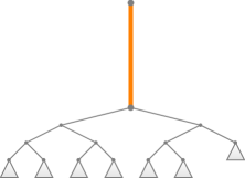
Figure 5: Bad instance for the cluster decomposition in [BP19]. Let $m=2\lceil\frac{1}{\delta}\rceil+1$, where $\delta=\Theta(\epsilon)$ is defined in [BP19]. Let the number of terminals in the tree be $2k$. The $2k$ terminals belong to $m$ subtrees of $2k/m$ terminals each (assuming that $2k$ is a multiple of $m$). Each of the $m$ subtrees (represented by a triangle) is a leaf cluster according to the decomposition in [BP19]. The unique edge incident to the root vertex (thick orange edge) has weight 1, and all other edges in the tree have weight 0. The optimal solution consists of two tours (each visiting exactly $k$ vertices), thus has cost 4. When the violation of tour capacity is not allowed and when each leaf cluster is required to be visited by a single tour, the solution contains at least 3 tours, hence a cost of at least 6.

Appendix B Proof of Lemma 9

A leaf component is a subtree rooted at a vertex $v\in V$ containing at least $\Gamma\cdot k$ terminals and such that each of the subtrees rooted at the children of $v$ contains strictly less than $\Gamma\cdot k$ terminals. Observe that the leaf components are disjoint subtrees of $T$. The backbone of $T$ is the partial subtree of $T$ consisting of all edges on paths from the root of $T$ to the root of some leaf component.

Definition 34 (key vertices).

We say that a vertex $v\in V$ is a key vertex if $v$ is of one of the three cases: (1) the root of a leaf component; (2) a branch point of the backbone; (3) the root of the tree $T$.

We say that two key vertices $v_{1},v_{2}$ are consecutive if the $v_{1}$-to-$v_{2}$ path in the tree does not contain any other key vertex. For each pair of consecutive key vertices $(v_{1},v_{2})$, we consider the subgraph between $v_{1}$ and $v_{2}$, and decompose that subgraph into internal components, each of demand at most $2\Gamma\cdot k$, such that all of these components are big (i.e., of demand at least $\Gamma\cdot k$) except for the upmost component.

A formal description of the construction is given in Algorithm 5. The first three properties in the claim follow from the construction.

Algorithm 5 Decomposition into components.

1:for each vertex $v\in V$ do

2:     $T(v)\leftarrow$ subtree of $T$ rooted at $v$

3:     $n(v)\leftarrow$ number of terminals in $T(v)$

4:for each non-leaf vertex $v\in V$ do

5:     Let $v_{1}$ and $v_{2}$ denote the two children of $v$ in $T$

6:     if $n(v)\geq\Gamma\cdot k$ and $n(v_{1})<\Gamma\cdot k$ and $n(v_{2})<\Gamma\cdot k$ then

7:         Let $T(v)$ be a leaf component with root vertex $v$      

8:

9:$B\leftarrow$ set of key vertices $\triangleright$ Definition 34

10:for each vertex $v_{2}\in B$ such that $v_{2}\neq r$ do

11:     $v_{1}\leftarrow$ lowest ancestor of $v_{2}$ among vertices in $B$ $\triangleright$ $v_{1}$ and $v_{2}$ are consecutive key vertices

12:     for each vertex $v$ on the $v_{1}$-to-$v_{2}$ path do $H(v)\leftarrow(T(v)\setminus T(v_{2}))\cup\{v_{2}\}$      

13:     $x\leftarrow v_{2}$

14:     while $H(v_{1})$ contains at least $\Gamma\cdot k$ terminals do

15:         $v\leftarrow$ the deepest vertex on the $v_{1}$-to-$x$ path such that $H(v)$ contains at least $\Gamma\cdot k$ terminals

16:         Let $H(v)$ be an internal component with root vertex $v$ and exit vertex $x$

17:         $x\leftarrow v$

18:         for each vertex $v^{\prime}$ on the $v_{1}$-to-$x$ path do $H(v^{\prime})\leftarrow(T(v^{\prime})\setminus T(x))\cup\{x\}$               

19:     if $v_{1}\neq x$ then

20:         Let $H(v_{1})$ be an internal component with root vertex $v_{1}$ and exit vertex $x$      

It remains to show the last property in the claim. For each big component $c$, we define the image of $c$ to be itself. It remains to consider the components that are not big, called bad components. Observe that the root vertex $r_{c}$ of any bad component $c$ is a key vertex. We say that a bad component $c$ is a left bad component (resp. right bad component) if $c$ contains the left child (resp. right child) of $r_{c}$. We define a map from left bad components to leaf components, such that the image of a left bad component is the leaf component that is rightmost among its descendants, and we show that this map is injective. Let $c_{1}$ and $c_{2}$ be any left bad components. Observe that $r_{c_{1}}$ and $r_{c_{2}}$ are distinct key vertices. If $r_{c_{1}}$ is ancestor of $r_{c_{2}}$ (the case when $r_{c_{2}}$ is ancestor of $r_{c_{1}}$ is similar), then the image of $c_{2}$ is in the left subtree of $r_{c_{2}}$ whereas the image of $c_{1}$ is outside the left subtree of $r_{c_{2}}$, so the images of $c_{1}$ and of $c_{2}$ are different. In the remaining case, the subtrees rooted at $r_{c_{1}}$ and at $r_{c_{2}}$ are disjoint, so the images of $c_{1}$ and of $c_{2}$ are different. Thus the map for left bad components is injective. Note that every leaf component is big. Therefore, we obtain an injective map from left bad components to big components such that the image of a left bad component is among its descendants. The map for right bad components is symmetric. Hence the first part of the last property. The second part of the last property follows from the first part of that property and the fact that the number of components with demands at least $\Gamma$ is at most $1/\Gamma$ times the total demand in the tree $T$. This completes the proof of the claim.

References

- [ACL10] Anna Adamaszek, Artur Czumaj, and Andrzej Lingas. PTAS for -tour cover problem on the plane for moderately large values of . International Journal of Foundations of Computer Science, 21(06):893–904, 2010.
- [AG90] Kemal Altinkemer and Bezalel Gavish. Heuristics for delivery problems with constant error guarantees. Transportation Science, 24(4):294–297, 1990.
- [AGM16] S. P. Anbuudayasankar, K. Ganesh, and Sanjay Mohapatra. Models for practical routing problems in logistics. Springer, 2016.
- [AKK01] Tetsuo Asano, Naoki Katoh, and Kazuhiro Kawashima. A new approximation algorithm for the capacitated vehicle routing problem on a tree. Journal of Combinatorial Optimization, 5(2):213–231, 2001.
- [AKTT97] Tetsuo Asano, Naoki Katoh, Hisao Tamaki, and Takeshi Tokuyama. Covering points in the plane by -tours: towards a polynomial time approximation scheme for general . In Proceedings of the twenty-ninth annual ACM symposium on Theory of computing, pages 275–283, 1997.
- [BDO06] Agustín Bompadre, Moshe Dror, and James B. Orlin. Improved bounds for vehicle routing solutions. Discrete Optimization, 3(4):299–316, 2006.
- [Bec18] Amariah Becker. A tight 4/3 approximation for capacitated vehicle routing in trees. In Approximation, Randomization, and Combinatorial Optimization. Algorithms and Techniques (APPROX/RANDOM), volume 116 of LIPIcs, pages 3:1–3:15, Dagstuhl, Germany, 2018. Schloss Dagstuhl–Leibniz-Zentrum fuer Informatik.
- [BKS17] Amariah Becker, Philip N. Klein, and David Saulpic. A quasi-polynomial-time approximation scheme for vehicle routing on planar and bounded-genus graphs. In 25th Annual European Symposium on Algorithms (ESA 2017). Schloss Dagstuhl-Leibniz-Zentrum fuer Informatik, 2017.
- [BKS18] Amariah Becker, Philip N. Klein, and David Saulpic. Polynomial-time approximation schemes for -center, -median, and capacitated vehicle routing in bounded highway dimension. In 26th Annual European Symposium on Algorithms (ESA 2018). Schloss Dagstuhl-Leibniz-Zentrum fuer Informatik, 2018.
- [BKS19] Amariah Becker, Philip N. Klein, and Aaron Schild. A PTAS for bounded-capacity vehicle routing in planar graphs. In Workshop on Algorithms and Data Structures, pages 99–111. Springer, 2019.
- [BP19] Amariah Becker and Alice Paul. A framework for vehicle routing approximation schemes in trees. In Workshop on Algorithms and Data Structures, pages 112–125. Springer, 2019.
- [BTV21] Jannis Blauth, Vera Traub, and Jens Vygen. Improving the approximation ratio for capacitated vehicle routing. In International Conference on Integer Programming and Combinatorial Optimization, pages 1–14. Springer, 2021.
- [CFKL20] Vincent Cohen-Addad, Arnold Filtser, Philip N. Klein, and Hung Le. On light spanners, low-treewidth embeddings and efficient traversing in minor-free graphs. In 2020 IEEE 61st Annual Symposium on Foundations of Computer Science (FOCS), pages 589–600. IEEE, 2020.
- [CL12] Teodor G. Crainic and Gilbert Laporte. Fleet management and logistics. Springer Science & Business Media, 2012.
- [DM15] Aparna Das and Claire Mathieu. A quasipolynomial time approximation scheme for Euclidean capacitated vehicle routing. Algorithmica, 73(1):115–142, 2015.
- [DR59] George B. Dantzig and John H. Ramser. The truck dispatching problem. Management Science, 6(1):80–91, 1959.
- [FMRS21] Zachary Friggstad, Ramin Mousavi, Mirmahdi Rahgoshay, and Mohammad R. Salavatipour. Improved approximations for CVRP with unsplittable demands. arXiv preprint arXiv:2111.08138, 2021.
- [GRW08] Bruce Golden, S. Raghavan, and Edward Wasil. The vehicle routing problem: latest advances and new challenges, volume 43 of Operations Research/Computer Science Interfaces Series. Springer, 2008.
- [GW81] Bruce L. Golden and Richard T. Wong. Capacitated arc routing problems. Networks, 11(3):305–315, 1981.
- [HK98] Shin-ya Hamaguchi and Naoki Katoh. A capacitated vehicle routing problem on a tree. In International Symposium on Algorithms and Computation, pages 399–407. Springer, 1998.
- [HR85] Mordecai Haimovich and Alexander H. G. Rinnooy Kan. Bounds and heuristics for capacitated routing problems. Mathematics of Operations Research, 10(4):527–542, 1985.
- [JS22] Aditya Jayaprakash and Mohammad R. Salavatipour. Approximation schemes for capacitated vehicle routing on graphs of bounded treewidth, bounded doubling, or highway dimension. In ACM-SIAM Symposium on Discrete Algorithms (SODA), pages 877–893, 2022.
- [KD16] Michael Khachay and Roman Dubinin. PTAS for the Euclidean capacitated vehicle routing problem in . In International Conference on Discrete Optimization and Operations Research, pages 193–205. Springer, 2016.
- [LLM91] Martine Labbé, Gilbert Laporte, and Hélene Mercure. Capacitated vehicle routing on trees. Operations Research, 39(4):616–622, 1991.
- [MZ22] Claire Mathieu and Hang Zhou. A tight -approximation for unsplittable capacitated vehicle routing on trees. https://arxiv.org/abs/2202.05691, 2022.
- [TV02] Paolo Toth and Daniele Vigo. The Vehicle Routing Problem. Society for Industrial and Applied Mathematics, 2002.