Controller Reduction for Nonlinear Systems by Generalized Differential Balancing

Abstract

In this paper, we aim at developing computationally tractable methods for nonlinear model/controller reduction. Recently, model reduction by generalized differential (GD) balancing has been proposed for nonlinear systems with constant input-vector fields and linear output functions. First, we study incremental properties in the GD balancing framework. Next, based on these analyses, we provide GD LQG balancing and GD $H_{\infty}$-balancing as controller reduction methods for nonlinear systems by focusing on linear feedback and observer gains. Especially for GD $H_{\infty}$-balancing, we clarify when the closed-loop system consisting of the full-order system and a reduced-order controller is exponentially stable. All provided methods for controller reduction can be relaxed to linear matrix inequalities.

I Introduction

An important but difficult challenge for model/controller reduction of nonlinear systems is to establish computationally tractable methods while guaranteeing stability properties of reduced-order systems/systems controlled by reduced-order controllers. Most of existing methods focus on one aspect; see e.g. [1, 2, 3, 4, 5] for computational tractability and e.g.,[6, 7, 8, 9, 10, 11] for theoretical analysis. A few papers [12, 13, 14, 15] aim at balancing these two. It is worth emphasizing that these papers study model reduction only. In contrast to linear systems [16, 17, 18, 19], controller reduction has been rarely studied for nonlinear systems. A few papers [20, 21] proceed with theoretical analysis based on solutions to Hamilton-Jacobi equations/inequalities (HJE/HJI). As well recognized, solving HJE/HJI is a computationally challenging problem.

As computationally tractable nonlinear model reduction methods with theoretical analysis, generalized incremental (GI) balancing [12] and generalized differential (GD) balancing [13] are proposed for nonlinear systems with constant input-vector fields and linear output functions, in the contraction [22, 23, 24, 25, 26, 27, 28, 29] and incremental stability [30] frameworks, respectively. However, in GD balancing [13], the main focus is not on the original systems, but their variational systems. In other words, properties of the full/reduced-order original (i.e. non-variational) systems are not well studied in GD balancing [13].

Toward developing controller reduction methods for nonlinear systems in the GD balancing framework, the first objective in this paper is to study incremental stability (IS) properties [23, 30] (i.e. stability properties of any pair of trajectories) for the original system based on GD balancing. We show that a system admitting a GD controllability Gramian is incrementally exponentially stable as a control system, and a similar statement holds for a GD observability Gramian. The IS properties guaranteed by this paper are preserved under model reduction by GD balanced truncation. Moreover, an upper bound on the reduction error is estimated. Note that [12] for GI balancing does not study a convergence between a pair of trajectories.

GD balancing is applicable only for stable systems. In the linear case, linear quadratic Gaussian (LQG) balanced truncation [16, 17] is known to be a model reduction method for unstable systems. The second objective in this paper is to extend LQG balancing in the GD balancing framework; the proposed approach is called GD LQG balancing. As for linear systems, GD LQG balancing has strong connections with GD coprime factorizations proposed in this paper, as extensions of coprime factorizations. As a byproduct of GD LQG balancing analysis with GD coprime factorizations, we present an observer-based dynamic stabilizing controller while the separation principle does not hold for nonlinear systems in general. This dynamic controller raises the question of whether its reduced-order controller stabilizes the full-order system. However, the answer is not clear even in the linear case while there are researches in this direction [16, 17].

For stabilizing reduced-order control design, $H_{\infty}$-balancing has been proposed for linear systems [18] and extended to nonlinear systems [20, 21] with HJE/HJI. The last and main objective of this paper is to develop GD $H_{\infty}$-balancing based on GD balancing and GD LQG balancing. The main difference from [20, 21] is that the proposed method can be achieved by solving sets of linear matrix inequalities instead of nonlinear partial differential equations/inequalities. In other words, this paper can be viewed as the first paper that provides a computationally tractable method for controller reduction of nonlinear systems while guaranteeing the stability of the closed-loop systems consisting of the full-order systems and reduced-order controllers. Such analyzable and computationally tractable methods are developed by focusing on linear feedback and observer gains.

The remainder of this paper is organized as follows. In Section II, we proceed with IS analysis of GD balancing. In Sections III and IV, GD LQG balancing and GD $H_{\infty}$-balancing are developed, respectively. Proposed methods are illustrated by means of examples in Section V. Concluding remarks are given in Section VI. All proofs are shown in Appendices.

Notation: The sets of real numbers and nonnegative real numbers are denoted by ${\mathbb{R}}$ and ${\mathbb{R}}_{+}$, respectively. For symmetric $P\in{\mathbb{R}}^{n\times n}$, $\lambda_{\max}(P)$ denotes its maximum eigenvalue. The inequality $P\succ 0$ ($P\succeq 0$) means that $P$ is symmetric and positive (semi) definite. For a vector $x\in{\mathbb{R}}^{n}$, the weighted norm by a matrix $P\succ 0$ is denoted by $|x|_{P}:=\sqrt{x^{\top}Px}$. If $P$ is identity, this is simply denoted by $|x|$. Also, the $\infty$-norm is denoted by $|x|_{\infty}:=\max_{i=1,\dots,n}|x_{i}|$. For a signal $u:{\mathbb{R}}_{+}\to{\mathbb{R}}^{m}$, the $L_{2}$-norm is denoted by $\|u\|:=(\int_{0}^{\infty}|u(t)|^{2}dt)^{1/2}$. The set of signals $u$ for which $(\int_{a}^{b}|u(t)|^{2}dt)^{1/2}$ (resp. $\sup_{t\in[a,b]}|u(t)|_{\infty}$) is bounded, is denoted by $L_{2}^{m}[a,b]$ (resp. $L_{\infty}^{m}[a,b]$). We define another set of signals by ${\mathcal{U}}:=\{\int_{0}^{t}v(\tau)d\tau:v\in L_{2}^{m}[0,\infty)\}\cap L_{\infty}^{m}[0,\infty)$.

II Generalized Differential Balancing

In this section, we proceed with analysis of generalized differential (GD) balancing [13, 9]. In particular, we study incremental stability properties based on a so-called GD controllability/observability Gramian. Then, we establish the bridge between those GD Gramians and incremental energy functions. After that, we study GD balanced truncation and provide an upper error bound for model reduction.

II-A Generalized Differential Gramians

Consider the system:

$$\left\{\begin{array}[]{l}\dot{x}=f(x)+Bu,\\ y=Cx,\end{array}\right.$$ (3)

where $x(t)\in{\mathbb{R}}^{n}$, $u(t)\in{\mathbb{R}}^{m}$, and $y(t)\in{\mathbb{R}}^{p}$ denote the state, input, and output, respectively. The function $f:{\mathbb{R}}^{n}\to{\mathbb{R}}^{n}$ is of class $C^{1}$, $B\in{\mathbb{R}}^{n\times m}$, and $C\in{\mathbb{R}}^{p\times n}$. Let $\phi(t,x_{0},u)$ denote the solution $x(t)$ to the system (3) at time $t\in{\mathbb{R}}_{+}$ starting from $x(0)=x_{0}\in{\mathbb{R}}^{n}$ with $u(t)\in{\mathbb{R}}^{m}$. Note that if $u(\cdot)$ is continuous, the solution $\phi(t,x_{0},u)$ is a class $C^{1}$ function of $t$ and $x_{0}$ as long as it exists.

The differential balancing framework is developed by using the system (3) and its variational system:

$$\left\{\begin{array}[]{l}\dot{\delta x}=\partial f(x)\delta x+B\delta u,\\ \delta y=C\delta x,\end{array}\right.$$ (6)

where $\delta x(t)\in{\mathbb{R}}^{n}$, $\delta u(t)\in{\mathbb{R}}^{m}$, and $\delta y(t)\in{\mathbb{R}}^{p}$ denote the state, input, and output of the variational system, respectively, and $\partial f(x):=\partial f(x)/\partial x$, $x\in{\mathbb{R}}^{n}$.

Using the variational system, a GD controllability Gramian and GD observability Gramian are respectively defined as solutions $X\succ 0$ and $Y\succ 0$ ($X,Y\in{\mathbb{R}}^{n\times n}$) to the following GD Lyapunov inequalities for $\varepsilon\geq 0$:

$$\partial f(x)X+X\partial^{\top}f(x)+BB^{\top}+\varepsilon X\preceq 0, \;\;\forall x\in{\mathbb{R}}^{n},$$ (7)

$$Y\partial f(x)+\partial^{\top}f(x)Y+C^{\top}C+\varepsilon Y\preceq 0, \;\;\forall x\in{\mathbb{R}}^{n}.$$ (8)

The above inequalities look like slight extensions of the original definitions of GD Gramians [13, 9], where $\varepsilon=0$ is assumed. However, our main interest is in the case $\varepsilon>0$. In this case, we can guarantee stability properties of the system (3) based on the GD Gramians (i.e., based on the variational system (6)), as is investigated in the next subsection.

At present, the existence of each GD Gramian is not clear. For another GD Lyapunov inequality, [26, Proposition 3] shows that an IES system admits a matrix-valued solution. It is not yet clear when this becomes a constant. On the other hand, there can be multiple GD controllability/observability Gramians. In bounded real or positive real balancing, the corresponding Riccati equations admit multiple solutions, and the concept of the minimal and maximal solutions have been introduced [31]. However, for the inequalities, the minimal or maximal solutions may not exist because the inequality relaxation makes the class of solutions wider, which allows us to impose additional requirements for model reduction such as structure-preservation; see e.g. Remark II.12 below.

II-B Incremental Stability Analysis

In the original work for differential balancing, properties of variational systems are investigated [13, 9]. As known in contraction analysis [23, 24], properties of variational systems have strong connections with incremental properties, i.e., system properties stated in terms of a pair of trajectories. In this section, we investigate incremental stability (IS) by using GD Gramians. To this end, we use the auxiliary system [30] consisting of the system (3) and its copy:

$$\left\{\begin{array}[]{ll}\dot{x}=f(x)+Bu,\\ \dot{x}^{\prime}=f(x^{\prime})+Bu^{\prime},\\ y=Cx,\\ y^{\prime}=Cx^{\prime}.\end{array}\right.$$ (13)

First, we recall the definition of incremental exponential stability as a property of trajectories $(x(t),x^{\prime}(t))$ of the auxiliary system for the same input $u(t)=u^{\prime}(t)$.

Definition II.1 (​​[23, 30])

The system (3) is said to be incrementally exponentially stable (IES) (with respect to $u(t)\in{\mathbb{R}}^{m}$) if $\phi(t,x_{0},u)\in{\mathbb{R}}^{n}$ for each $x_{0}\in{\mathbb{R}}^{n}$ and $t\in{\mathbb{R}}_{+}$, and there exist $k,\lambda>0$ such that

$$|\phi(t,x_{0},u)-\phi(t,x^{\prime}_{0},u)|\leq ke^{-\lambda t}|x_{0}-x^{\prime}_{0}|,\;\forall t\in{\mathbb{R}}_{+},$$

for any $(x_{0},x^{\prime}_{0})\in{\mathbb{R}}^{n}\times{\mathbb{R}}^{n}$. $\lhd$

Now, we are ready to state the first result. Thanks to newly introduced $\varepsilon>0$, IS properties can be studied by using the GD controllability Gramian, differently from the existing works for GD balancing [13, 9].

Theorem II.2

Given $\varepsilon>0$, if the system (3) has a GD controllability Gramian $X\succ 0$, then

1. $|\phi(t,x_{0},u)-\phi(t,x^{\prime}_{0},u^{\prime})|$, $t\in{\mathbb{R}}_{+}$ exists for any $(x_{0},x^{\prime}_{0})\in{\mathbb{R}}^{n}\times{\mathbb{R}}^{n}$ and $(u,u^{\prime})$ such that $u-u^{\prime}\in L_{2}^{m}[0,\infty)$ and $u^{\prime}\in{\mathcal{U}}$;

2. $\lim_{t\to\infty}|\phi(t,x_{0},u)-\phi(t,x^{\prime}_{0},u^{\prime})|=0$ for any $(x_{0},x^{\prime}_{0})\in{\mathbb{R}}^{n}\times{\mathbb{R}}^{n}$ and $(u,u^{\prime})\in{\mathcal{U}}\times{\mathcal{U}}$ such that $u-u^{\prime}\in L_{2}^{m}[0,\infty)$;

3. the system is IES with respect to each $u\in{\mathcal{U}}$;

4. for each constant input $u=u^{*}\in{\mathbb{R}}^{m}$, the system has the globally exponentially stable (GES) equilibrium point $x^{*}\in{\mathbb{R}}^{n}$;

5. for each $x_{0}\in{\mathbb{R}}^{n}$ and $u\in L_{2}^{m}[0,\infty)$, $|\phi(t,x_{0},u)|$ is a bounded function of $t\in{\mathbb{R}}_{+}$. $\lhd$

Remark II.3

As can be noticed from the proof of Theorem II.2, the condition $u\in{\mathcal{U}}$ (resp. $u^{\prime}\in{\mathcal{U}}$) can be replaced with $u\in L_{2}^{m}[0,\infty)$ (resp. $u^{\prime}\in L_{2}^{m}[0,\infty)$) in items 1) – 3). $\lhd$

We have a similar result for observability.

Theorem II.4

Given $\varepsilon>0$, if the system (3) has a GD observability Gramian $Y\succ 0$, then

1. $|\phi(t,x_{0},u^{*})-\phi(t,x^{\prime}_{0},u^{*})|$, $t\in{\mathbb{R}}_{+}$ exists for any $(x_{0},x^{\prime}_{0})\in{\mathbb{R}}^{n}\times{\mathbb{R}}^{n}$ and $u^{*}\in{\mathbb{R}}^{m}$;

2. for each constant input $u=u^{*}\in{\mathbb{R}}^{m}$, the system is IES and has the GES equilibrium point $x^{*}\in{\mathbb{R}}^{n}$. $\lhd$

Remark II.5

In contraction analysis of autonomous systems, a considered set (${\mathbb{R}}^{n}$ in this case) is typically assumed to be positively invariant, see e.g., [23, 25, 26]. However, we do not assume that ${\mathbb{R}}^{n}$ is robustly positively invariant [32] (positive invariance as a control system) in Theorems II.2 and II.4. Namely, IES is guaranteed without any assumption for positive invariance. Furthermore, we can conclude that the system has a unique equilibrium point for each constant input, which is also a new finding of this paper. These are benefits of newly introduced $\varepsilon>0$. In fact, this is the first paper studying IES in the balancing framework. In particular, there is no study for IS properties based on a controllability Gramian other than Theorem II.2; even the paper [12] on generalized incremental balancing has not studied IS properties. Only a statement similar to that of item 1) in Theorem II.4 for an observability Gramian is found in [12, Lemma 2]. In other words, item 2) is also a new finding of this paper. $\lhd$

Remark II.6

Even when $\varepsilon=0$, item 1) of each Theorems II.2 and II.4 can be shown. Moreover, the existence of a GD observability Gramian $Y\succ 0$ for $\varepsilon=0$ implies

$$\lim_{t\to\infty}|y(t)-y^{\prime}(t)|=0$$

for each constant input $u=u^{\prime}=u^{*}$. In addition, if the system has the detectability property:

$$\lim_{t\to\infty}|u(t)-u^{\prime}(t)|=0,\;\lim_{t\to\infty}|y(t)-y^{\prime}(t)|=0$$

$$\hskip 14.22636pt\implies\lim_{t\to\infty}|\phi(t,x_{0},u)-\phi(t,x^{\prime}_{0},u^{\prime})|=0,$$ (14)

then $\lim_{t\to\infty}|\phi(t,x_{0},u)-\phi(t,x^{\prime}_{0},u^{\prime})|=0$ is guaranteed. $\lhd$

The inequality (7) or (8) is not only helpful for studying stability properties, but also characterizes structures of the mapping $f$ itself.

Corollary II.7

Given $\varepsilon>0$, if either (7) or (8) holds, then $f:{\mathbb{R}}^{n}\to{\mathbb{R}}^{n}$ is a globally diffeomorphism. $\lhd$

II-C Connections with Incremental Energy Functions

Linear/nonlinear balancing has a strong connection with the so-called controllability and observability functions [33, 6]. By using the auxiliary system, define the following incremental controllability and observability functions, respectively,

$$J_{u}(x_{0},x^{\prime}_{0}):=\inf_{\begin{subarray}{c}u-u^{\prime}\in L_{2}^{m}[0,\infty)\\ (x(0),x^{\prime}(0))=(x_{0},x^{\prime}_{0})\\ x(-\infty)=x^{\prime}(-\infty)\end{subarray}}\int_{-\infty}^{0}|u(t)-u^{\prime}(t)|^{2}dt,$$ (15)

and

$$J_{y}(x_{0},x^{\prime}_{0},u^{*}) :=\int_{0}^{\infty}|y(t)-y^{\prime}(t)|^{2}dt,$$ (16)

$$(x(0),x^{\prime}(0))=(x_{0},x^{\prime}_{0}),\;u=u^{\prime}=u^{*}\in{\mathbb{R}}^{m}.$$

Remark II.8

The incremental controllability and observability functions (15) and (16) are slightly different from those in [8]. When compared to the incremental controllability function based on the sum $u+u^{\prime}$ in [8, Definition 6], (15) can be regarded in a more natural incremental function as the difference $u-u^{\prime}$ is considered (and we do not require additionally $x(-\infty)=x^{\prime}(-\infty)=0$). The incremental observability function in [8, Definition 5] is defined as the supremum over all input functions. $\lhd$

A GD controllability/observability Gramian naturally provides a lower/upper bound on these incremental energy functions, as is stated next.

Theorem II.9

Consider the system (3) and its auxiliary system (13). Suppose that

1. $J_{u}(x_{0},x^{\prime}_{0})$ in (15) exists for any $(x_{0},x^{\prime}_{0})\in{\mathbb{R}}^{n}\times{\mathbb{R}}^{n}$;

2. given $\varepsilon\geq 0$, a GD controllability Gramian $X\succ 0$ exists.

Then,

$$|x_{0}-x^{\prime}_{0}|_{X^{-1}}^{2}\leq J_{u}(x_{0},x^{\prime}_{0})$$ (17)

for any $(x_{0},x^{\prime}_{0})\in{\mathbb{R}}^{n}\times{\mathbb{R}}^{n}$. $\lhd$

Theorem II.10

Consider the system (3) and its auxiliary system (13). Suppose that

1. $J_{y}(x_{0},x^{\prime}_{0},u^{*})$ in (16) exists for some constant input $u^{*}\in{\mathbb{R}}^{m}$ and for any $(x_{0},x^{\prime}_{0})\in{\mathbb{R}}^{n}\times{\mathbb{R}}^{n}$;

2. given $\varepsilon\geq 0$, a GD observability Gramian $Y\succ 0$ exists;

3. the system (3) has the detectability property (14).

Then,

$$J_{y}(x_{0},x^{\prime}_{0},u^{*})\leq|x_{0}-x^{\prime}_{0}|_{Y}^{2}$$ (18)

for any $(x_{0},x^{\prime}_{0})\in{\mathbb{R}}^{n}\times{\mathbb{R}}^{n}$. $\lhd$

II-D Model Reduction

GD balanced truncation has been developed based on the following proposition. Originally, this is shown for $\varepsilon=0$ [13, Theorem 19.17], but holds for each $\varepsilon\geq 0$.

Proposition II.11

Given $\varepsilon\geq 0$, if a system (3) has both GD controllability and observability Gramians $X\succ 0$ and $Y\succ 0$, then there exist GD balanced coordinates in which

$$X=Y=\Sigma:={\rm diag}\{\sigma_{1},\dots,\sigma_{n}\},\;\sigma_{1}\geq\cdots\geq\sigma_{n}>0$$

hold. $\lhd$

A change of coordinates $z=Tx$ into GD balanced coordinates can be constructed similarly as for balanced coordinates between the controllability and observability Gramians of linear systems [34, 33]. Hereafter in this subsection, suppose that the system (3) has both positive definite GD controllability and observability Gramians $X$ and $Y$. For the sake of simplicity of the description, we further suppose that a realization (3) is GD balanced, namely $X=Y=\Sigma$.

For $r$ satisfying $\sigma_{r}>\sigma_{r+1}$, define

$$\Sigma_{1}:={\rm diag}\{\sigma_{1},\dots,\sigma_{r}\},\;\Sigma_{2}:={\rm diag}\{\sigma_{r+1},\dots,\sigma_{n}\}.$$ (19)

Correspondingly, we divide the system (3) into

$$x=\begin{bmatrix}x_{1}\\ x_{2}\end{bmatrix},\;f(x)=\begin{bmatrix}f_{1}(x_{1},x_{2})\\ f_{2}(x_{1},x_{2})\end{bmatrix},\;B=\begin{bmatrix}B_{1}\\ B_{2}\end{bmatrix},$$

$$C=\begin{bmatrix}C_{1}&C_{2}\end{bmatrix}.$$ (20)

A reduced-order model by GD balancing is constructed as

$$\left\{\begin{array}[]{l}\dot{x}_{r}=f_{1}(x_{r}+c_{1},c_{2})+B_{1}u,\\ y_{r}=C_{1}(x_{r}+c_{1})+C_{2}c_{2},\end{array}\right.$$ (23)

where $c:=[c_{1}^{\top}c_{2}^{\top}]^{\top}\in{\mathbb{R}}^{n}$ is arbitrary.

In the balanced coordinates, $\Sigma$ is both GD controllability and observability Gramians. Namely, the system (20) satisfies (7) and (8) for $X=Y=\Sigma$. Now, the GD Lyapunov inequality (7) becomes

$$\begin{bmatrix}\partial_{x_{1}}f_{1}&\partial_{x_{2}}f_{1}\\ \partial_{x_{1}}f_{2}&\partial_{x_{2}}f_{2}\end{bmatrix}\begin{bmatrix}\Sigma_{1}&0\\ 0&\Sigma_{2}\end{bmatrix}+\begin{bmatrix}\Sigma_{1}&0\\ 0&\Sigma_{2}\end{bmatrix}\begin{bmatrix}\partial_{x_{1}}f_{1}&\partial_{x_{2}}f_{1}\\ \partial_{x_{1}}f_{2}&\partial_{x_{2}}f_{2}\end{bmatrix}^{\top}$$

$$+\begin{bmatrix}B_{1}B_{1}^{\top}&B_{1}B_{2}^{\top}\\ B_{1}B_{2}^{\top}&B_{2}B_{2}^{\top}\end{bmatrix}+\varepsilon\begin{bmatrix}\Sigma_{1}&0\\ 0&\Sigma_{2}\end{bmatrix}\preceq 0,$$

where $\partial_{x_{i}}f_{j}:=\partial f_{j}/\partial x_{i}$, $i,j=1,2$. From the $(1,1)$-th block diagonal element, one notices that $\Sigma_{1}\succ 0$ is a GD controllability Gramian for the reduced-order model (23). A similar discussion holds for a GD observability Gramian. Therefore, similar statements as Theorems II.2 and II.4 hold for the reduced-order model. That is, GD balanced truncation preserves stability properties.

Remark II.12

As mentioned in the previous subsection, there can be multiple GD Gramians. This is beneficial, for instance, for structure-preserving model reduction. Consider the interconnection of two subsystems:

$$\left\{\begin{array}[]{l}\dot{x}_{1}=f_{1}(x_{1})+g_{1}(x_{2})+B_{1}u_{1},\\ \dot{x}_{2}=g_{2}(x_{1})+f_{2}(x_{2})+B_{2}u_{2},\\ y_{1}=C_{1}x_{1},\;y_{2}=C_{2}x_{2}.\end{array}\right.$$

If we specify the structures of GD Gramians $X$ and $Y$ as block-diagonal matrices, i.e. $X={\rm diag}\{X_{1},X_{2}\}$ and $Y={\rm diag}\{Y_{1},Y_{2}\}$ with the compatible dimensions, then we can achieve model reduction of each subsystem separately, which preserves the interconnection structure. $\lhd$

An error between the full-order system and reduced-order model can be estimated for a specific drift vector field. In fact, a similar error bound can be established by combining [8, Theorem 3] and [8, Theorem 18]. However, our result is more general, and the proof is used later in analysis of controller reduction.

Theorem II.13

Suppose that

1. given $\varepsilon\geq 0$, the system (3) has both GD controllability and observability Gramians $X\succ 0$ and $Y\succ 0$;

2. $\sigma_{r}>\sigma_{r+1}$;

3. in GD balanced coordinates, there exists $c\in{\mathbb{R}}^{n}$ such that $f(x_{r}+c_{1},c_{2})=-f(-x_{r}+c_{1},c_{2})$ for all $x_{r}\in{\mathbb{R}}^{r}$.

Then, the outputs of the system (3) and its reduced-order model (23) satisfy

$$\|y-y_{r}\|\leq 2\sum_{i=r+1}^{n}\sigma_{i}\|u\|.$$ (24)

for any $u\in L_{2}^{m}[0,\infty)$ under the initial states $x(0)=c$ and $x_{r}(0)=0$. $\lhd$

Remark II.14

In Theorem II.13, if $\varepsilon>0$, the constant $c$ can be chosen as zero without loss of generality. First, item 4) of Theorem II.2 for $u=0$ implies that there exists a unique equilibrium $x^{*}$. Next, for $x_{r}=0$, the condition in item III) of Theorem II.13 becomes $2f(c_{1},c_{2})=0$, which implies $c=x^{*}$. In the new coordinates $\hat{x}:=x-x^{*}$, the equilibrium point is zero, and the condition in item III) of Theorem II.13 holds for $c=0$. On the other hand, in the $\hat{x}$-coordinates, the output becomes an affine function $y=C(\hat{x}+x^{*})$. However, one can define the new outputs $\hat{y}:=y-Cx^{*}=C\hat{x}$. Note that the GD Gramians do not depend on the shifts of coordinates $\hat{x}=x-x^{*}$ and outputs $\hat{y}=y-Cx^{*}$, since the variational system (6) is independent from them. $\lhd$

Hereafter, to reduce the complexity of discussions, we impose the following without loss of generality.

Standing Assumption II.15

$f(0)=0$ in (3) and $c=0$ in (23). $\lhd$

Remark II.16

Under $f(0)=0$, if (7) has a solution $X\succ 0$ on a convex set $D\subset{\mathbb{R}}^{n}$ containing the origin, then any trajectory starting from $D$ with the zero input converges to the origin. More generally, as long as $\phi(t,x_{0},u)\in D$, $t\in{\mathbb{R}}_{+}$, the trajectory converges to the origin for any $x_{0}\in D$ and $u\in{\mathcal{U}}$. Therefore, the obtained results for GD balancing in this section can be extended to model reduction on $D$. $\lhd$

Under Assumption II.15, item III) of Theorem II.13 requires that $f$ is an odd function. That is, each $f_{i}$, $i=1,\dots,n$ is odd. Odd nonlinearities naturally appear in physical systems such as nonlinear pendulums [35], ball and beam systems [36], mass-spring-damper systems with hardening springs [35], and van der Pol oscillators (or more generally negative resistance oscillators) [35]. Moreover, relays and saturations, standard static nonlinearities [35] can be approximated by $\arctan(x)$ that is an odd function.

Note that we assume $f$ to be odd in error analysis of model reduction and later in controller reduction to guarantee the stability of the closed-loop system with a reduced-order controller. Otherwise, this assumption is not required. In fact, (7) and (8) can have solutions without this assumption. Consider the following scaler system: $\dot{x}=-x-x^{2}-x^{3}+u$, where $f$ is not odd. One can confirm that $X=2$ is a solution to (7) for $\varepsilon=0.1$.

III Generalized Differential LQG Balancing

As balanced truncation for linear systems is applicable only for stable systems, GD balancing requires that the system (3) has IS properties. For unstable linear/nonlinear systems, so-called LQG balancing has been proposed [16, 37, 17]. In this section, to deal with non-IES systems, we develop a new LQG balancing method in the GD balancing framework, which we call GD LQG balancing. Next, inspired by results on LQG balancing, we also propose GD coprime factorizations and investigate its GD balancing in terms of GD LQG balancing of the system (3). Based on the results on coprime factorizations, we study stabilizing dynamic controller design.

III-A Generalized Differential Riccati Equations

Motivated by LQG balancing [16, 37, 17], we consider the following past energy function,

$$J_{-}(x_{0},x^{\prime}_{0})=\inf_{\begin{subarray}{c}u-u^{\prime}\in L_{2}^{m}(-\infty,0]\\ (x(0),x^{\prime}(0))=(x_{0},x^{\prime}_{0})\\ x(-\infty)=x^{\prime}(-\infty)\end{subarray}}\int_{-\infty}^{0}\eta(t)dt,$$ (25)

and post energy function,

$$J_{+}(x_{0},x^{\prime}_{0})=\inf_{\begin{subarray}{c}u-u^{\prime}\in L_{2}^{m}[0,\infty)\\ (x(0),x^{\prime}(0))=(x_{0},x^{\prime}_{0})\\ x(\infty)=x^{\prime}(\infty)\end{subarray}}\int_{0}^{\infty}\eta(t)dt,$$ (26)

where $\eta(t):=|y(t)-y^{\prime}(t)|^{2}+|u(t)-u^{\prime}(t)|^{2}$.

As done for the incremental controllability/observability function in the previous section, we first estimate their lower/upper bound by using each solution $P\succ 0$ or $Q\succ 0$ ($P$, $Q\in{\mathbb{R}}^{n\times n}$) to the following GD control Riccati inequality or GD filter Riccati inequality for $\varepsilon\geq 0$:

$$P\partial f(x)+\partial^{\top}f(x)P -PBB^{\top}P$$

$$+C^{\top}C+\varepsilon P\preceq 0,\;\forall x\in{\mathbb{R}}^{n},$$ (27)

$$\partial f(x)Q+Q\partial^{\top}f(x) -QC^{\top}CQ$$

$$+BB^{\top}+\varepsilon Q\preceq 0,\;\forall x\in{\mathbb{R}}^{n}.$$ (28)

An upper bound on $J_{+}(x_{0},x^{\prime}_{0})$ can be estimated by using the GD control Riccati inequality (27) as stated below.

Theorem III.1

For the system (3) and its auxiliary system (13), suppose that

1. $J_{+}(x_{0},x^{\prime}_{0})$ in (26) exists for any $(x_{0},x^{\prime}_{0})\in{\mathbb{R}}^{n}\times{\mathbb{R}}^{n}$;

2. given $\varepsilon\geq 0$, the GD control Riccati inequality (27) admits a solution $P\succ 0$;

3. the system has the detectability property (14).

Then,

$$J_{+}(x_{0},x^{\prime}_{0})\leq|x_{0}-x^{\prime}_{0}|_{P}^{2}$$ (29)

for any $(x_{0},x^{\prime}_{0})\in{\mathbb{R}}^{n}\times{\mathbb{R}}^{n}$. $\lhd$

A similar result is obtained for a lower bound on $J_{-}(x_{0},x^{\prime}_{0})$ and the GD filter Riccati inequality (28) as stated below.

Theorem III.2

For the system (3) and its auxiliary system (13), suppose that

1. $J_{-}(x_{0},x^{\prime}_{0})$ in (25) exists for any $(x_{0},x^{\prime}_{0})\in{\mathbb{R}}^{n}\times{\mathbb{R}}^{n}$;

2. given $\varepsilon\geq 0$, the GD filter Riccati inequality (28) admits a solution $Q\succ 0$.

Then

$$|x_{0}-x^{\prime}_{0}|_{Q^{-1}}^{2}\leq J_{-}(x_{0},x^{\prime}_{0})$$ (30)

for any $(x_{0},x^{\prime}_{0})\in{\mathbb{R}}^{n}\times{\mathbb{R}}^{n}$. $\lhd$

If GD Riccati inequalities (27) and (28) have solutions $P\succ 0$ and $Q\succ 0$, respectively, then as for GD Gramians $X,Y\succ 0$, there exist coordinates, named GD LQG balanced coordinates, in which

$$P=Q=\Pi:={\rm diag}\{\pi_{1},\dots,\pi_{n}\},$$ (31)

$$\pi_{1}\geq\cdots\geq\pi_{n}>0.$$

Let $\pi_{r}>\pi_{r+1}$, and define $\Pi_{1}:={\rm diag}\{\pi_{1},\dots,\pi_{r}\}$. Then, in the GD LQG balanced coordinates, model reduction of the system (3) can be achieved in a similar manner as GD balancing. Furthermore, $\Pi_{1}$ satisfies both GD Riccati inequalities (27) and (28) for the reduced-order model (23).

Finally, it is remarked that the GD controllability and observability Gramians $X$ and $Y$ satisfy the GD Riccati inequalities (28) and (27), respectively. This implies that GD LQG balancing can be applied to a wider class of systems than GD balancing.

III-B Generalized Differential Right Coprime Representations

LQG balancing has been understood as balanced truncation of the so-called right coprime representation, i.e. the closed-loop system designed by the stabilizing solution to the control Riccati equation [37, 17]. Motivated by this, we define a GD right coprime representation (RCR) with a solution $P\succ 0$ to the GD control Riccati inequality (27) as follows:

$$\left\{\begin{array}[]{l}\dot{x}=f(x)-BB^{\top}Px+Bv,\\ \begin{bmatrix}y\\ u\end{bmatrix}=\begin{bmatrix}C\\ -B^{\top}P\end{bmatrix}x+\begin{bmatrix}0\\ I_{m}\end{bmatrix}v,\end{array}\right.$$ (34)

where $v(t)\in{\mathbb{R}}^{m}$ is the new input.

Similarly to the linear case, both GD controllability and observability Gramians for the GD RCR are constructed from solutions to the GD Riccati inequalities (27) and (28) as stated below.

Theorem III.3

Consider the system (3). Suppose that given $\varepsilon\geq 0$, the GD Riccati inequalities (27) and (28) admit solutions $P\succ 0$ and $Q\succ 0$, respectively. Then, $(P+Q^{-1})^{-1}$ (resp. $P$) is a GD controllability (resp. observability) Gramian of the GD RCR (34). $\lhd$

Remark III.4

Theorem III.3 implies that the GD RCR (34) satisfies similar statements as Theorems II.2 and II.4 for stability. That is, $u=-B^{\top}Px$ is a stabilizing controller of the system (3) if $\varepsilon>0$. In fact, in Theorem III.1, the detectability property is not necessarily if $\varepsilon>0$. $\lhd$

From Theorem III.3, GD LQG balanced coordinates of the system (3) are also GD balanced coordinates of the GD RCR (34). Indeed, from (31), it follows that

$$(P+Q^{-1})^{-1}=(\Pi+\Pi^{-1})^{-1}$$

$$={\rm diag}\{\pi_{1}/(1+\pi_{1}^{2}),\dots,\pi_{n}/(1+\pi_{n}^{2})\}.$$

Therefore, in GD LQG balanced coordinates, the GD controllability Gramian $(\Pi+\Pi^{-1})^{-1}$ and GD observability Gramian $\Pi$ of the GD RCR (34) are diagonal. In these coordinates, one can achieve GD balanced truncation of the GD RCR. A reduced-order model of the GD RCR is a GD RCR of the reduced-order model (23), i.e., a constructing reduced order model and computing a GD RCR are commutative. Furthermore, an error bound for GD balanced truncation of the GD RCR can be estimated as in Theorem II.13.

III-C Generalized Differential Left Coprime Representations

Next, we consider an extension of the left coprime representation (LCR) [37, 17], which is defined by using a solution $Q\succ 0$ to the GD Riccati inequality (28) as follows:

$$\left\{\begin{array}[]{l}\dot{x}=f(x)-QC^{\top}Cx+\begin{bmatrix}B&QC^{\top}\end{bmatrix}\begin{bmatrix}u\\ y\end{bmatrix},\\ z=Cx+\begin{bmatrix}0&-I_{p}\end{bmatrix}\begin{bmatrix}u\\ y\end{bmatrix},\end{array}\right.$$ (37)

where $z(t)\in{\mathbb{R}}^{p}$ is the new output.

As for the GD RCR, both GD controllability and observability Gramians of the GD LCR are obtained from the GD Riccati inequalities (27) and (28) as follows.

Theorem III.5

Consider the system (3). Suppose that given $\varepsilon\geq 0$, the GD Riccati inequalities (27) and (28) admit solutions $P\succ 0$ and $Q\succ 0$, respectively. Then, $Q$ (resp. $(Q+P^{-1})^{-1}$) is a GD controllability (resp. observability) Gramian of the GD LCR (37). $\lhd$

GD LQG balanced coordinates of the system (3) are also GD balanced coordinates for the GD LCR (37). Therefore, one can achieve GD balanced truncation, and the obtained reduced-order model is a GD LCR of the reduced-order model (23).

As briefly mentioned in Remark III.4, the GD RCR (34) corresponds to the closed-loop system with a stabilizing controller $u=-B^{\top}Px$. In fact, the GD LCR (37) corresponds to observer dynamics. Consider the following system having the same dynamics as the GD LCR:

$$\dot{\hat{x}}=f(\hat{x})-QC^{\top}C\hat{x}+\begin{bmatrix}B&QC^{\top}\end{bmatrix}\begin{bmatrix}u\\ y\end{bmatrix}.$$ (38)

If its initial state is the same as the initial state of the system (3), i.e., $\hat{x}(0)=x_{0}$, then $\hat{x}=x$. Therefore, if (38) is IES with respect to the external inputs $(u,y)$, then $\hat{x}(t)-x(t)\to 0$ as $t\to\infty$ for arbitrary $x_{0}$, $\hat{x}(0)\in{\mathbb{R}}^{n}$, which implies that (38) is an observer of (3). If $\varepsilon>0$, the IES of (38) can be shown by combining Theorems II.2 and III.5.

III-D Dynamic Stabilizing Controllers

As mentioned in the previous subsections, the GD RCR and LCR correspond to a static stabilizing controller and observer, respectively. Thus, it is expected that a dynamic stabilizing controller can be constructed by combining them. In this subsection, we show that this is true even though the separation principle does not hold for nonlinear systems in general.

As a dynamic controller, we consider the following observer based stabilizing controller:

$$\left\{\begin{array}[]{l}\dot{x}_{c}=f(x_{c})+Bu-QC^{\top}(Cx_{c}-y),\\ u=-B^{\top}Px_{c}.\end{array}\right.$$ (41)

The closed-loop system consisting of (3) and (41) is

$$\left\{\begin{array}[]{l}\dot{x}=f(x)-BB^{\top}Px_{c},\\ \dot{x}_{c}=f(x_{c})-BB^{\top}Px_{c}-QC^{\top}C(x_{c}-x).\end{array}\right.$$ (44)

This closed-loop system is stable, which is stated formally.

Theorem III.6

Consider the system (3). Suppose that given $\varepsilon>0$, the GD Riccati inequalities (27) and (28) admit solutions $P\succ 0$ and $Q\succ 0$, respectively. Then, the closed-loop system (44) is GES at the origin (recall Assumption II.15).  $\lhd$

Since $\Pi_{1}$ satisfies both GD Riccqti inequalities (27) and (28) for the reduced-order model (23) (constructed by GD LQG balancing), the following controller:

$$\left\{\begin{array}[]{l}\dot{x}_{cr}=f_{1}(x_{cr},0)-B_{1}u-\Pi_{1}C_{1}^{\top}(C_{1}x_{cr}-y_{r}),\\ u=-B_{1}^{\top}\Pi_{1}x_{cr},\end{array}\right.$$

is a dynamic stabilizing controller of the reduced-order model (23) with $c=0$. Then, one may ask whether this reduced-order controller stabilizes the full-order system (3). However, the answer is not very clear even in the linear case while there are researches in this direction, e.g., [16, 17]. Toward designing a reduced-order stabilizing controller, in the next section, we develop another balancing method as an extension of $H_{\infty}$-balancing [18].

IV Generalized Differential $H_{\infty}$-Balancing

In this section, we extend the so-called $H_{\infty}$-balancing in the GD balancing framework. The objective is to design a reduced-order controller which stabilizes the system (3). We first design a full-order dynamic stabilizing controller and then consider reducing its dimension while guaranteeing closed-loop stability.

IV-A Full-Order Dynamic Controller Design

Now, we consider the generalized plant corresponding to the system (3):

$$G:\left\{\begin{array}[]{l}\dot{x}=f(x)+Bu+Bw_{u},\\ z_{u}=u,\\ z_{y}=Cx,\\ y=Cx+w_{y},\end{array}\right.$$ (49)

where $w(t):=[w_{u}^{\top}(t)\;w_{y}^{\top}(t)]^{\top}\in{\mathbb{R}}^{m+p}$ and $z:=[z_{u}^{\top}(t)\;z_{y}^{\top}(t)]^{\top}\in{\mathbb{R}}^{m+p}$.

The first goal is to design an output feedback controller solving a standard $L_{2}$ ($H_{\infty}$) control problem [38, 39].

Problem IV.1

For the system (49), find a controller such that

1. the $L_{2}$-gain of the closed-loop system from $w$ to $z$ is not greater than a prescribed value $\gamma>1$, namely $\|z\|\leq\gamma\|w\|$ for the zero initial state;

2. the closed-loop system is GES at the origin when $w=0$ (recall Assumption II.15). $\lhd$

This problem can be solved by the following procedure. Define

$$\beta:=\sqrt{1-\gamma^{-2}}>0.$$ (50)

First, given $\varepsilon\geq 0$, we find a solution $P_{\infty}\succ 0$ ($P_{\infty}\in{\mathbb{R}}^{n\times n}$) to the following GD Riccati inequality:

$$P_{\infty}\partial f(x)+\partial^{\top}f(x)P_{\infty}-\beta^{2}P_{\infty}BB^{\top}P_{\infty}$$

$$+C^{\top}C+\varepsilon P_{\infty}\preceq 0,\;\forall x\in{\mathbb{R}}^{n}.$$ (51)

This corresponds to the $H_{\infty}$-control algebraic Riccati equation in the linear case. Similarly, one can infer a counterpart of the $H_{\infty}$-filter algebraic Riccati equation (HFARE). However, when an equality is relaxed to an inequality, we need a modification to solve Problem IV.1; a similar modification can be found in the Hamilton-Jacobi approach [39]. In fact, we use a lower bound on the left-hand side of (51), namely the following $R_{\infty}(x)\succeq 0$ ($R_{\infty}(x)\in{\mathbb{R}}^{n\times n}$), $x\in{\mathbb{R}}^{n}$:

$$-R_{\infty}(x)\preceq \;P_{\infty}\partial f(x)+\partial^{\top}f(x)P_{\infty}-\beta^{2}P_{\infty}BB^{\top}P_{\infty}$$

$$+C^{\top}C+\varepsilon P_{\infty},\;\forall x\in{\mathbb{R}}^{n}.$$ (52)

Then, we consider the following inequality for $Q_{\infty}\succ 0$ ($Q_{\infty}\in{\mathbb{R}}^{n\times n}$) as an extension of HFARE:

$$\partial f(x)Q_{\infty}+Q_{\infty}\partial^{\top}f(x)-\beta^{2}Q_{\infty}C^{\top}CQ_{\infty}$$

$$+BB^{\top}+\varepsilon Q_{\infty}\preceq-\gamma^{-2}Q_{\infty}R_{\infty}(x)Q_{\infty},\;\forall x\in{\mathbb{R}}^{n}.$$ (53)

As the first result of this section, we show that if the above GD Riccati inequalities (51) and (53) have solutions, then Problem IV.1 can be solved.

Theorem IV.2

For the system (49), suppose that

1. given $\varepsilon\geq 0$, the GR Riccati inequality (51) admits a solution $P_{\infty}\succ 0$;

2. for $R_{\infty}(x)\succeq 0$, $x\in{\mathbb{R}}^{n}$ satisfying (52), the GR Riccati inequality (53) admits a solution $Q_{\infty}\succ 0$;

3. $\gamma^{2}>\lambda_{\max}(P_{\infty}Q_{\infty})$.

Then, the following dynamic controller solves item 1) of Problem IV.1:

$$K:\left\{\begin{array}[]{l}\dot{x}_{c}=f(x_{c})-\beta^{2}BB^{\top}P_{\infty}x_{c}\\ \hskip 28.45274pt-(Q_{\infty}^{-1}-\gamma^{-2}P_{\infty})^{-1}C^{\top}(Cx_{c}-y),\\ u=-B^{\top}P_{\infty}x_{c}.\end{array}\right.$$ (57)

Moreover, if $\varepsilon>0$, this controller solves item 2) of Problem IV.1. $\lhd$

Next, we investigate the connection between the $L_{2}$-gain of the closed-loop system $\gamma>0$ and $\varepsilon>0$. It is possible to show that $\gamma$ can be made smaller by selecting a smaller $\varepsilon$.

Theorem IV.3

For the system (49), suppose that items I) – III) of Theorem IV.2 hold for $\varepsilon>0$. Next, consider $\varepsilon_{1},\varepsilon_{2}>0$ and $0<\alpha<\beta^{2}$ such that $\varepsilon=\varepsilon_{1}+2\varepsilon_{2}$ and

$$\alpha P_{\infty}BB^{\top}P_{\infty}\preceq\varepsilon_{2}P_{\infty},$$ (58)

$$\alpha Q_{\infty}C^{\top}CQ_{\infty}\preceq\varepsilon_{2}Q_{\infty}.$$ (59)

Then, $P_{\infty}$, $\bar{R}_{\infty}(x):=R_{\infty}(x)+\varepsilon_{2}P_{\infty}$, and $Q_{\infty}$ satisfy (51), (52), and (53) for $\bar{\gamma}:=\gamma/\sqrt{1+\alpha\gamma^{2}}$, respectively. $\lhd$

Theorem IV.3 implies that $\gamma$ can be made smaller by finding $\alpha>0$ and $\varepsilon_{2}>0$ under the constraints (58), (59), $\alpha<\beta^{2}$, and $2\varepsilon_{2}<\varepsilon$. Namely, the GD Riccati inequalities (51) and (53) hold for $\gamma=\bar{\gamma}$ if such $\alpha$ and $\varepsilon_{2}$ exist. Finding $\alpha$ and $\varepsilon_{2}$ can be formulated as a convex problem by relaxing $>$ to $\geq$ with a small positive constant. Furthermore, the maximum $\alpha$ can be computed. A larger $\alpha$ gives a smaller $\bar{\gamma}$, and a small $\gamma$ is beneficial to reduce the dimension of a controller while guaranteeing closed-loop stability as will be clear in Theorem IV.4. Moreover, for the new $\gamma=\bar{\gamma}$, we can again solve the GD Riccati inequalities to obtain better solutions, e.g., for reducing the dimension of a stabilizing controller.

IV-B Controller Reduction

As for GD balancing/LQG balancing, if the GD Riccati inequalities (51) and (53) have solutions $P_{\infty}\succ 0$ and $Q_{\infty}\succ 0$, respectively, then there exist coordinates, named GD $H_{\infty}$-balanced coordinates, in which

$$P_{\infty}=Q_{\infty}=\Pi:={\rm diag}\{\pi_{1},\dots,\pi_{n}\},$$ (60)

$$\pi_{1}\geq\cdots\geq\pi_{n}>0,$$

where we use the same symbol $\Pi$ as GD LQG balancing by abuse of notation. Let $\pi_{r}>\pi_{r+1}$, and define $\Pi_{1}:={\rm diag}\{\pi_{1},\dots,\pi_{r}\}$. Hereafter, suppose that the realization (49) is GD $H_{\infty}$-balanced. Then, in a similar manner as GD balancing/GD LQG balancing, a reduced-order model of the generalized plant (49) can be constructed as follows:

$$G_{r}:\left\{\begin{array}[]{l}\dot{x}_{r}=f_{1}(x_{r},0)+B_{1}u+B_{1}w_{ur},\\ z_{ur}=u,\\ z_{yr}=y_{r}=C_{1}x_{r},\\ y=C_{1}x_{r}+w_{yr},\end{array}\right.$$ (65)

where $w_{r}(t):=[w_{ur}^{\top}(t)\;w_{yr}^{\top}(t)]^{\top}\in{\mathbb{R}}^{m+p}$ and $z_{r}(t):=[z_{ur}^{\top}(t)\;z_{yr}^{\top}(t)]^{\top}\in{\mathbb{R}}^{m+p}$. For the sake of later analysis, we use different symbols from $w$ and $z$.

Note that $\Pi_{1}$ satisfies both GD Riccati inequalities (51) and (53) for the reduced-order model (65), where the $(1,1)$-th block diagonal element of $R_{\infty}(x)$ in the GD $H_{\infty}$-balanced coordinates is considered. Moreover, $\gamma^{2}>\lambda_{\max}(P_{\infty}Q_{\infty})=\lambda_{\max}(\Pi^{2})=\pi_{1}^{2}$ implies $\gamma^{2}>\lambda_{\max}(\Pi_{1}^{2})=\pi_{1}^{2}$. Therefore, if all conditions in Theorem IV.2 and $\pi_{r}>\pi_{r+1}$ hold, the following reduced-order controller solves Problem IV.1 for the reduced-order model (65):

$$K_{r}:\left\{\begin{array}[]{l}\dot{x}_{cr}=f_{1}(x_{cr},0)-\beta^{2}B_{1}B_{1}^{\top}\Pi_{1}x_{cr}\\ \hskip 28.45274pt-(\Pi_{1}^{-1}-\gamma^{-2}\Pi_{1})^{-1}C_{1}^{\top}(C_{1}x_{cr}-y),\\ u=-B_{1}^{\top}\Pi_{1}x_{cr}.\end{array}\right.$$ (69)

If this reduced-order controller satisfies some additional conditions, the closed-loop system consisting of the full-order plant (49) and reduced-order controller (69), denoted by $\Gamma(G,K_{r})$, is exponentially stable. The following theorem is the main result of this section, and the next subsection is dedicated to proving this.

Theorem IV.4

For the system (49), suppose that

1. items I) – III) of Theorem IV.2 hold;

2. $\pi_{r}>\pi_{r+1}$;

3. $f$ is an odd function;

4. $\rho_{r}(1+\gamma\beta^{-1})<1$, where

   $$\rho_{r}:=2\sum_{i=r+1}^{n}\frac{\beta\pi_{i}}{\sqrt{1+\beta^{2}\pi_{i}^{2}}}.$$ (70)

Then, the following holds.

1. the closed-loop system $\Gamma(G,K_{r})$ consisting of the full-order plant (49) and reduced-order controller (69) satisfies

   $$\|z\|\leq\beta^{-1}\frac{\beta\gamma+\rho_{r}(\gamma+\beta)}{\beta-\rho_{r}(\gamma+\beta)}\|w\|$$ (71)

   for the initial states $x(0)=0$ and $x_{r}(0)=0$.

Furthermore, if $\varepsilon>0$ and $w=0$, then

1. $\Gamma(G,K_{r})$ is GES at the origin. $\lhd$

Remark IV.5

Even in the linear case, there is no inequality relaxation of $H_{\infty}$-balancing. Therefore, Theorem IV.4 is a new result even for linear systems. $\lhd$

Item IV) of Theorem IV.4 can be useful for deciding the dimension $r$ of a reduced-order controller. Given $\gamma>0$, (50) determines $\beta$. Then, $\pi_{i}$ is obtained by solving the GD Riccati inequalities (51) and (53) and by computing GD $H_{\infty}$-balanced coordinates as in (60). Thus, $r$ is only the design parameter in item IV) of Theorem IV.4. The smallest $r$ satisfying the condition is the lowest dimension of a reduced-order controller for which Theorem IV.4 guarantees the closed-loop stability.

Note that our methods are based on matrix inequalities (51) – (53). They can be reduced into linear matrix inequalities (LMIs). For instance, consider (51) and define $\hat{P}_{\infty}:=P_{\infty}^{-1}$. Multiplying $P_{\infty}^{-1}$ from both sides leads to the following LMIs for $\hat{P}_{\infty}$:

$$\left\{\begin{array}[]{l}\hat{P}_{\infty}\succ 0,\\ \begin{bmatrix}\partial f(x)\hat{P}_{\infty}+\hat{P}_{\infty}\partial^{\top}f(x)-\beta^{2}BB^{\top}+\varepsilon\hat{P}_{\infty}&\hat{P}_{\infty}C^{\top}\\ C\hat{P}_{\infty}&-I\end{bmatrix}\preceq 0.\end{array}\right.$$ (74)

This consists of an infinite family of LMIs for each fixed $x\in{\mathbb{R}}^{n}$. An approximation solution can be constructed for instance by taking finite sampling points $x_{(i)}\in{\mathbb{R}}^{n}$, $i=1,\dots,D$. To find an exact solution, a convex relaxation can be used. Let ${\mathbb{A}}:=\{A_{1},\dots,A_{L}\}\subset{\mathbb{R}}^{n\times n}$ be a family of matrices such that

$$\partial f(x)\in{\rm ConvexHull}({\mathbb{A}}),\;\forall x\in{\mathbb{R}}^{n}.$$ (75)

Then, any solution $\hat{P}_{\infty}\in{\mathbb{R}}^{n\times n}$ to the following matrix inequalities

$$\left\{\begin{array}[]{l}\hat{P}_{\infty}\succ 0,\\ \begin{bmatrix}A_{i}\hat{P}_{\infty}+\hat{P}_{\infty}A_{i}^{\top}-\beta^{2}BB^{\top}+\varepsilon\hat{P}_{\infty}&\hat{P}_{\infty}C^{\top}\\ C\hat{P}_{\infty}&-I\end{bmatrix}\preceq 0,\\ \hskip 170.71652pti=1,\dots,L.\end{array}\right.$$ (79)

satisfies (74). Indeed, from (75), for each $x\in{\mathbb{R}}^{n}$, there exist $\theta_{i}(x)\geq 0$, $i=1,\dots,L$ such that $\partial f(x)=\sum_{i=1}^{L}\theta_{i}(x)A_{i}$ and $\sum_{i=1}^{L}\theta_{i}(x)=1$. Then, multiplying $\theta_{i}(x)$ by the second LMI of (79) and taking the summation for $i=1,\dots,L$ lead to (74).

The set of LMIs (79) can have multiple solutions $\hat{P}_{\infty}$, but our results hold for all solutions. In controller reduction, $P_{\infty}$ having small eigenvalues is useful to guarantee the stability of the closed-loop system with a reduced-order controller. Since $\hat{P}_{\infty}$ corresponds to $P^{-1}_{\infty}$, a reasonable approach is to find $\hat{P}_{\infty}$ having the largest trace. This can be formulated as a convex optimization problem.

Similar statements hold for (52) and (53). Therefore, our methods can be applied by solving finite families of LMIs. In other words, we do not need to solve nonlinear partial differential equations/inequalities differently from existing nonlinear controller reduction methods such as [20, 21]. Depending on the system, $L$ can be large. However, the problem is still convex. In general, solving a convex (optimization) problem is more tractable than that of a nonlinear partial differential equation/inequality. We have similar remarks for GD balancing and GD LQG balancing.

Remark IV.6

A convex relaxation can be utilized for local model/controller reduction. As mention in Remark II.16, under $f(0)=0$, results of GD balancing can be delivered to a convex subset, and this is also true for GD LQG balancing and GD $H_{\infty}$-balancing. Furthermore, the mentioned convex relaxation is always doable on a bounded set, since $\partial f(x)$ is bounded on it. Therefore, we can always utilize the convex relaxation for model/controller reduction on a bounded convex set. $\lhd$

The convex relaxation mentioned above is one approach. Even if $\partial f(x)$ is not bounded, a convex relaxation can be applied depending on problems. For instance, consider $\dot{x}=-x-x^{3}+u$, where $\partial f(x)=-1-3x^{2}$ is not bounded. In this case, we can still find a solution to (7) by solving an LMI. The GD Lyapunov inequality (7) for $X>0$ becomes $2X(-1-3x^{2})+1+\varepsilon X\leq 0$. Since $-Xx^{2}\leq 0$ for all $x\in{\mathbb{R}}$, we only have to solve the following LMI: $-2X+1+\varepsilon X\leq 0$. A solution is for instance $X=1$ for $\varepsilon=0.1$.

IV-C Analysis for Proving Theorem IV.4

The goal of this subsection is to prove Theorem IV.4. The main idea is to utilize the small gain theorem by interpreting the closed-loop system $\Gamma(G,K_{r})$ as the feedback interconnection of the reduced-order closed-loop system (consisting of the reduced-order model (49) and reduced-order controller (69)), denoted by $\Gamma(G_{r},K_{r})$, and its perturbation $\Delta$ as in Fig. 1.

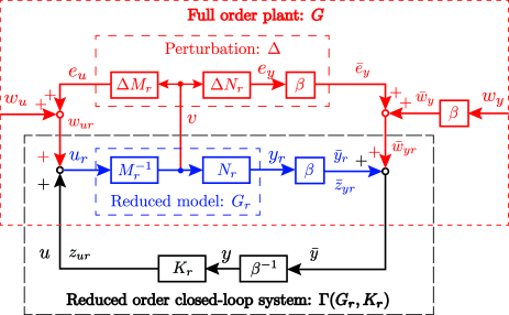
Figure 1: The closed-loop system $\Gamma(G,K_{r})$ consisting of the full-order plant (49) and reduced-order controller (69)

Throughout this subsection, suppose that a realization (49) is GD $H_{\infty}$-balanced, namely (60) holds. As a preliminary step, we summarize signals used in this subsection; also see Fig. 1.

$$w_{r} :=e+w,\;\bar{w}_{r}:=\bar{e}+\bar{w},$$

$$\bar{w}_{y} :=\beta w_{y},\;\bar{w}_{yr}:=\beta w_{yr},\;\bar{e}_{y}:=\beta e_{y},$$

$$e :=\begin{bmatrix}e_{u}\\ e_{y}\end{bmatrix},\;\bar{e}:=\begin{bmatrix}e_{u}\\ \bar{e}_{y}\end{bmatrix},\;\bar{w}:=\begin{bmatrix}w_{u}\\ \bar{w}_{y}\end{bmatrix},\;\bar{w}_{r}:=\begin{bmatrix}w_{ur}\\ \bar{w}_{yr}\end{bmatrix},$$

$$u_{r} :=u+w_{ur}=z_{ur}+w_{ur},$$

$$\bar{y} :=\beta y,\;\bar{y}_{r}:=\beta y_{r},$$

$$y :=y_{r}+w_{yr}=z_{yr}+w_{yr}.$$ (80)

For the analysis of the feedback interconnection of $\Delta$ and $\Gamma(G_{r},K_{r})$, we estimate the gains of $\Delta:v\to\bar{e}$ and $\Gamma(G_{r},K_{r}):\bar{w}+\bar{e}\to v$. Then, the small gain theorem provides a stability condition for the interconnection. However, the definitions of $v$, $e$, and $\Delta$ are still missing. They are defined via a reduced-order model of the following system:

$$\left\{\begin{array}[]{l}\dot{x}=f(x)-\beta^{2}BB^{\top}P_{\infty}x+Bv,\\ \begin{bmatrix}\bar{z}_{y}\\ u\end{bmatrix}=\begin{bmatrix}\beta C\\ -\beta^{2}P_{\infty}\end{bmatrix}x+\begin{bmatrix}0\\ I_{m}\end{bmatrix}v.\end{array}\right.$$ (83)

This is a GD RCR of the system (3) with the weighted output $\bar{z}_{y}=\beta z_{y}=\beta Cx$ by $\beta$. As Theorem III.3 for GD LQG balancing, its reduced-order model can be computed by using GD $H_{\infty}$-balancing of the system (3); the proof is similar and thus is omitted.

Theorem IV.7

Consider the system (49). Suppose that given $\varepsilon\geq 0$, the GD Riccati inequalities (51) and (53) admit solutions $P_{\infty}\succ 0$ and $Q_{\infty}\succ 0$, respectively. Then, $(\beta^{2}P_{\infty}+Q_{\infty}^{-1})^{-1}$ (resp. $\beta^{2}P_{\infty}$) is a GD controllability (resp. observability) Gramian of the GD RCR (83). $\lhd$

From Theorem IV.7, in GD $H_{\infty}$-balanced coordinates of the system (49), the GD RCR (83) is also GD balanced (in the sense of Section II). Therefore, GD $H_{\infty}$-balanced truncation gives a GD balanced truncated reduced-order model of the GD RCR (83):

$$\left\{\begin{array}[]{l}\dot{x}_{r}=f_{1}(x_{r},0)-\beta^{2}B_{1}B_{1}^{\top}\Pi_{1}x_{r}+B_{1}v,\\ \begin{bmatrix}\bar{z}_{yr}\\ u_{r}\end{bmatrix}=\begin{bmatrix}\beta C_{1}\\ -\beta^{2}\Pi_{1}\end{bmatrix}x_{r}+\begin{bmatrix}0\\ I_{m}\end{bmatrix}v.\end{array}\right.$$ (86)

An important fact is that this is a GD RCR of the reduced-order model (65) with the weighted output $\bar{z}_{yr}=\beta z_{yr}=\beta C_{1}x_{r}$ by $\beta$.

Now, we are ready to introduce $v$, $e$, and $\Delta$ in Fig. 1. First, we decompose the reduced-order GD RCR (86) into two subsystems $M_{r}^{-1}:u_{r}\to v$ and $\beta N_{r}:v\to\bar{z}_{yr}$ found in Fig. 1 as follows:

$$M_{r}^{-1} :\left\{\begin{array}[]{l}\dot{x}_{r}=f_{1}(x_{r},0)+B_{1}u_{r},\\ v=\beta^{2}B_{1}^{\top}\Pi_{1}x_{r}+u_{r},\end{array}\right.$$ (89)

$$\beta N_{r} :\left\{\begin{array}[]{l}\dot{x}_{r}=f_{1}(x_{r},0)-\beta^{2}B_{1}B_{1}^{\top}\Pi_{1}x_{r}+B_{1}v,\\ \bar{z}_{yr}=\beta z_{yr}=\beta C_{1}x_{r},\end{array}\right.$$ (92)

where the initial states $x_{r}(0)$ of both subsystems are the same. One notices that their series interconnection $\beta N_{r}\circ M_{r}^{-1}$ is the reduced-order model (23) with the weighted output $\bar{z}_{yr}=\beta z_{yr}=\beta C_{1}x_{r}$ by $\beta$, denoted by $\beta G_{r}$ in Fig. 1.

Now, $v$ is obtained as the output of $M_{r}^{-1}$. To proceed with further analysis, we substitute

$$u_{r}=u+w_{ur}=-B_{1}^{\top}\Pi_{1}x_{cr}+w_{ur}$$

following from (69) and (80) into $v$. Then, $v$ is described as the output of the reduced-order closed-loop system $\Gamma(G_{r},K_{r})$:

$$v=-\beta^{2}B_{1}^{\top}\Pi_{1}(x_{cr}-x_{r})+w_{ur}.$$

According to the previous subsection, the gain from $w_{r}$ to $z_{r}$ of the reduced-order closed-loop system $\Gamma(G_{r},K_{r})$ is not greater than $\gamma$. Based on this, we can estimate an upper bound on the gain of $\Gamma(G_{r},K_{r}):\bar{w}_{r}\to v$ as stated below. For the sake of later analysis, we decompose $\bar{w}_{r}$ as $\bar{w}_{r}=\bar{w}+\bar{e}$, where $\bar{e}$ will be introduced later.

Lemma IV.8

For the system (49), suppose that items I) and II) of Theorem IV.4 hold. Then, for the reduced-order closed-loop system $\Gamma(G_{r},K_{r})$, it holds that

$$\|v\|\leq(1+\gamma\beta^{-1})\|\bar{w}_{r}\|\leq(1+\gamma\beta^{-1})(\|\bar{e}\|+\|\bar{w}\|)$$

for the initial states $x_{r}(0)=0$ and $x_{cr}(0)=0$. $\lhd$

Next, we estimate the gain of the perturbation $\Delta$ in Fig. 1 by using the GR RCR (83) and its reduced-order model (86) again. One notices that $\bar{e}_{y}=\bar{z}_{y}-\bar{z}_{yr}$ and $e_{u}=z_{u}-z_{ur}$, i.e.

$$\Delta:=\begin{bmatrix}\beta\Delta N_{r}&\Delta M_{r}\end{bmatrix}=\begin{bmatrix}\beta N-\beta N_{r}&M-M_{r}\end{bmatrix}.$$

Therefore, $\Delta$ can be represented as error dynamics between the GD RCR (83) and its reduced-order model (86). Since model reduction is achieved by GD balanced truncation, an error bound is obtained as a direct application of Theorems II.13 and IV.7 without the proof.

Corollary IV.9

For the system (49), suppose that items I) – III) of Theorem IV.4 hold. Then, for the GD RCR (83) and its reduced-order model (86), we have

$$\|\bar{e}\|\leq\rho_{r}\|v\|,\;\rho_{r}:=2\sum_{i=r+1}^{n}\frac{\beta\pi_{i}}{\sqrt{1+\beta^{2}\pi_{i}^{2}}},$$ (93)

where $x(0)=0$ and $x_{r}(0)=0$. $\lhd$

Now, upper bounds on the gains of $\Gamma(G_{r},K_{r}):\bar{w}+\bar{e}\to v$ and $\Delta:v\to\bar{e}$ are provided by Lemma IV.8 and Corollary IV.9, respectively. Therefore, the small gain theorem for their interconnection yields Theorem IV.4.

V Examples

V-A Model Reduction by Generalized Differential Balancing

In this subsection, model reduction by GD balanced truncation is illustrated by an example. Consider the following system:

$$\dot{x}_{1} =-3x_{1}+\sin(x_{2}-x_{1})+u,$$

$$\dot{x}_{i} =-3x_{i}+\sin(x_{i-1}-x_{i})+\sin(x_{i+1}-x_{i}),\;i\neq 1,n,$$

$$\dot{x}_{n} =-3x_{n}+\sin(x_{n-1}-x_{n}),$$

$$y =x_{1}.$$ (94)

Then, it follows that

$$\partial f(x)\in{\rm ConvexHull}(\{A_{0},A_{1},\dots,A_{2n-2}\}),\;\forall x\in{\mathbb{R}}^{n}$$

$$\hskip 11.38109ptA_{0}:={\rm diag}\{-3,\dots,-3\},\;K=\begin{bmatrix}1&-1\\ -1&1\end{bmatrix},$$

$$\hskip 11.38109ptA_{1}:=A_{0}+{\rm diag}\{K,0,\dots,0\},$$

$$\hskip 11.38109ptA_{2}:=A_{0}+{\rm diag}\{-K,0,\dots,0\},$$

$$\hskip 11.38109ptA_{3}:=A_{0}+{\rm diag}\{0,K,0,\dots,0\},$$

$$\hskip 11.38109ptA_{4}:=A_{0}+{\rm diag}\{0,-K,0,\dots,0\},\dots,$$

$$\hskip 11.38109ptA_{2n-3}:=A_{0}+{\rm diag}\{0,\dots,0,K\},$$

$$\hskip 11.38109ptA_{2n-2}:=A_{0}+{\rm diag}\{0,\dots,0,-K\}.$$

Since each $A_{i}$ is symmetric and $B=C^{\top}$, both GD controllability and observability Gramians can be chosen to be the same, i.e. $X=Y$.

We consider the case where $n=100$ and solve the GD Lyapunov inequality (7) with the convex relaxation. Since it is difficult to display a solution $X$ due to its size, its eigenvalues are plotted in Fig. 3. Also, the upper error bounds (24) for GD balanced truncation are plotted in Fig. 3. From the error bounds, it is expected that the error can be very large when the dimension of the reduced-order model is less than $5$. To confirm this, we conduct simulations of the output trajectories of the $100$-dimensional original system as well as $5$-dimensional and $2$-dimensional reduced-order models. Fig. 5 shows the output trajectories for $x(0)=0$, $x_{r}(0)=0$, and $u(t)=\sin(t)+\sin(3t)$. Fig. 5 shows the output trajectories for $x(0)=0$, $x_{r}(0)=0$, and $u(t)=1$. As expected, the $2$-dimensional reduced-order model has a different behavior from the original system in contrast to the $5$-dimensional one. In other words, for this specific example, a $100$-dimensional nonlinear system can accurately be approximated by a $5$-dimensional reduced-order model by GD balancing.

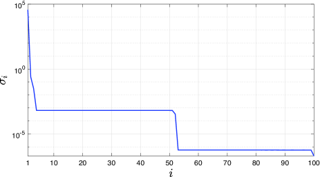
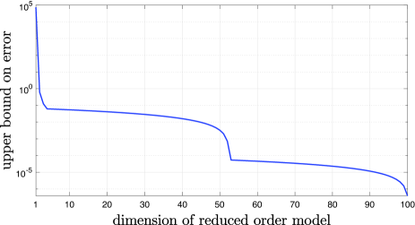
Figure 2: Eigenvalues of a GD controllability/observability Gramian

Figure 3: Upper bounds on model reduction error by GD balanced truncation

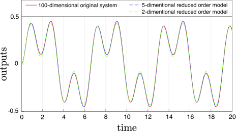
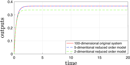
Figure 4: Output trajectories of the system (V-A) and its reduced order models when $x(0)=0$, $x_{r}(0)=0$, and $u(t)=\sin(t)+\sin(3t)$

Figure 5: Output trajectories of the system (V-A) and its reduced order models when $x(0)=0$, $x_{r}(0)=0$, and $u(t)=1$

V-B Controller Reduction by Generalized Differential $H_{\infty}$-Balancing

In this subsection, controller reduction based on GD $H_{\infty}$-balancing is illustrated by an example. Consider the following mechanical model controlled by a DC motor:

$$\left\{\begin{array}[]{l}\ddot{z}+c\dot{z}+k(z)=ai_{c},\\ L\dot{i}_{c}+Ri_{c}+k_{v}\dot{z}=u,\\ y=\begin{bmatrix}z&\dot{z}\end{bmatrix}^{\top},\end{array}\right.$$ (98)

where $z$ and $i_{c}$ denote the position of the mass and the current of the circuit, respectively. The control input $u$ is the voltage. The parameters are $c=2$, $a=1$, $L=1/5$, $R=1$, and $k_{v}=1$. The nonlinear function is chosen as $k(x)=-\sin z$. Then, $\partial k(z)/\partial z\in[-1,1]$ for all $z\in{\mathbb{R}}$.

We take the state as $x:=[z\;\dot{z}\;i_{c}]^{\top}$. To compute $P_{\infty}$ and $Q_{\infty}$, we use the convex relaxations like (79) with

$$A_{1} =\begin{bmatrix}0&1&0\\ 1&-2&1\\ 0&-5&-5\end{bmatrix},\;A_{2}=\begin{bmatrix}0&1&0\\ -1&-2&1\\ 0&-5&-5\end{bmatrix},\;B=\begin{bmatrix}0\\ 0\\ 5\end{bmatrix},$$

$$C =\begin{bmatrix}1&0&0\\ 0&1&0\end{bmatrix},$$

where $A_{1}$ is not Hurwitz.

Let $\gamma^{2}=2$. For $\varepsilon=0.01$, solutions to (79) and a similar relaxation of (53) are obtained as

$$P_{\infty} =\begin{bmatrix}3.20&0.888&0.163\\ 0.888&0.477&0.0778\\ 0.163&0.0778&0.0154\end{bmatrix},$$

$$Q_{\infty} =\begin{bmatrix}0.993&-0.0848&0.104\\ -0.0848&0.338&0.0737\\ 0.104&0.0737&2.43\end{bmatrix}.$$

Then, the matrix $\Pi$ in (60) is computed as follows:

$$\Pi={\rm diag}\{1.78,0.400,0.192\}.$$

The conditions in Theorem IV.4 hold for $r=2$, but not for $r=1$. Therefore, from Theorem IV.4, the system can be stabilized by the full-order or $2$-dimensional reduced-order controller. Fig. 6 shows the trajectories of the system controlled by the full-order or reduced-order controllers. Although Theorem IV.4 does not guarantee the stability for the $1$-dimensional reduced-order controller, all controllers stabilize the system in simulation. This implies that Theorem IV.4 can be conservative, since this theorem is derived based on the small gain theorem. Developing a less conservative stability condition is included in future work.

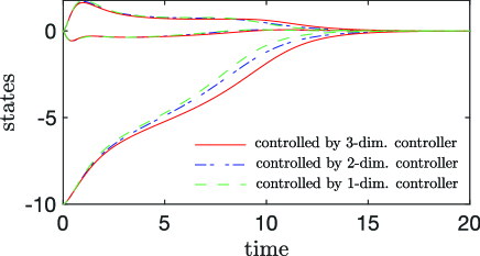
Figure 6: State trajectories of the system (98) controlled by controllers with different dimensions

VI Conclusion

In this paper, we have developed GD balancing methods. First, for GD balancing, we have shown that a nonlinear system admitting a GD controllability Gramian is IES as a control system and have estimated an upper error bound for GD balanced truncation. Next, we have proposed GD LQG balancing that has been studied relating to GD RCR/LCR. As a byproduct, we have obtained observer-based stabilizing controllers while the separation principle does not work for nonlinear systems in general. Finally, we have established GD $H_{\infty}$-balancing for controller reduction and presented a stability condition for the closed-loop system consisting of the full-order system and a reduced-order controller. These three GD balancing methods can be relaxed to LMIs. Future work includes extending the results of this paper to more general nonlinear systems by considering matrix-valued solutions to GD Lyapunov or Riccati inequalities.

Appendix A Proofs for GD Balancing

A-A Proof of Theorem II.2

Before proving each item, we show that for each input $u\in{\mathcal{U}}$, the solution to the system (3) exists. Using (7), compute

$$\frac{d}{dt}|f(x)+Bu|_{X^{-1}}^{2}$$

$$=(f(x)+Bu)^{\top}X^{-1}$$

$$\hskip 28.45274pt\times(\partial f(x)X+X\partial^{\top}f(x))X^{-1}(f(x)+Bu)$$

$$\hskip 11.38109pt+2\dot{u}^{\top}B^{\top}X^{-1}(f(x)+Bu)$$

$$\leq-|B^{\top}X^{-1}(f(x)+Bu)|_{2}-\varepsilon|f(x)+Bu|_{X^{-1}}^{2}$$

$$\hskip 11.38109pt+2\dot{u}^{\top}B^{\top}X^{-1}(f(x)+Bu)$$

$$=-\varepsilon|f(x)+Bu|_{X^{-1}}^{2}-|B^{\top}X^{-1}(f(x)+Bu)-\dot{u}|^{2}+|\dot{u}|^{2}$$

$$\leq-\varepsilon|f(x)+Bu|_{X^{-1}}^{2}+|\dot{u}|^{2}.$$

With the comparison principle [35, Lemma 3.4], the time integration over the interval $[0,t]$ yields

$$|f(x(t))+Bu(t)|_{X^{-1}}^{2}\leq \;e^{-\varepsilon t}|f(x(0))+Bu(0)|_{X^{-1}}^{2}$$

$$+\int_{0}^{t}e^{-\varepsilon(t-\tau)}|\dot{u}(\tau)|^{2}d\tau.$$ (99)

Therefore, $|\dot{x}(t)|=|f(x(t))+Bu(t)|$ is a bounded function of $t\in{\mathbb{R}}_{+}$ for each $u\in{\mathcal{U}}$. This implies that $|x(t)|$ exists for any $t\in{\mathbb{R}}_{+}$, but does not guarantee the boundedness of $|x(t)|$.

Now we are ready to prove each item.

Proof:

Consider the line segment $\gamma(s)=sx+(1-s)x^{\prime}$, $s\in[0,1]$. Then,

$$f(x)-f(x^{\prime}) =\int_{0}^{1}\frac{df(\gamma(s))}{ds}ds$$

$$=\int_{0}^{1}\partial f(\gamma(s))(x-x^{\prime})ds.$$ (100)

Using (7) and (100), similar computations as the previous give

$$\frac{d}{dt}|x-x^{\prime}|_{X^{-1}}^{2}$$

$$=2(x-x^{\prime})^{\top}X^{-1}(f(x)-f(x^{\prime})+B(u-u^{\prime}))$$

$$=\int_{0}^{1}(x-x^{\prime})^{\top}X^{-1}$$

$$\hskip 42.67912pt\times(\partial f(\gamma(s))X+X\partial^{\top}f(\gamma(s)))X^{-1}(x-x^{\prime})ds$$

$$\hskip 14.22636pt+2(x-x^{\prime})^{\top}X^{-1}B(u-u^{\prime})$$

$$\leq-|B^{\top}X^{-1}(x-x^{\prime})|^{2}-\varepsilon|x-x^{\prime}|_{X^{-1}}^{2}$$

$$\hskip 14.22636pt+2(u-u^{\prime})^{\top}B^{\top}X^{-1}(x-x^{\prime})$$

$$=-\big{|}u-u^{\prime}-B^{\top}X^{-1}(x-x^{\prime})\big{|}^{2}+|u-u^{\prime}|^{2}-\varepsilon|x-x^{\prime}|_{X^{-1}}^{2}$$

$$\leq-\varepsilon|x-x^{\prime}|_{X^{-1}}^{2}+|u-u^{\prime}|^{2}.$$ (101)

With the comparison principle, the time integration over the interval $[0,t]$ yields

$$|x(t)-x^{\prime}(t)|_{X^{-1}}^{2}\leq \;e^{-\varepsilon t}|x(0)-x^{\prime}(0)|_{X^{-1}}^{2}$$

$$+\int_{0}^{t}e^{-\varepsilon(t-\tau)}|u(\tau)-u^{\prime}(\tau)|^{2}d\tau.$$ (102)

Recall $x^{\prime}(t)=\phi(t,x^{\prime}_{0},u^{\prime})\in{\mathbb{R}}^{n}$, $t\in{\mathbb{R}}_{+}$ for each $x^{\prime}_{0}\in{\mathbb{R}}^{n}$ and $u^{\prime}\in{\mathcal{U}}$. Thus, (102) implies the statement of item 1). ∎

Proof:

The time integration of (101) over the interval $[0,t]$ yields

$$|x(t)-x^{\prime}(t)|_{X^{-1}}^{2}+\varepsilon\int_{0}^{t}|x(\tau)-x^{\prime}(\tau)|_{X^{-1}}^{2}d\tau$$

$$\leq|x_{0}-x^{\prime}_{0}|_{X^{-1}}^{2}+\int_{0}^{t}|u(\tau)-u^{\prime}(\tau)|^{2}d\tau,\;\forall\tau>0.$$ (103)

Since $\varepsilon>0$ and $u-u^{\prime}\in L_{2}^{m}[0,\infty)$, taking $\tau\to\infty$ implies $x-x^{\prime}\in L_{2}^{n}[0,\infty)$. Note that any $x(t)$ with $u\in{\mathcal{U}}$ is uniformly continuous with respect to $t\in{\mathbb{R}}_{+}$, since its derivative $\dot{x}(t)=f(x(t))+Bu(t)$ is bounded as shown in (99). Therefore, the statement of item 2) follows from Barbalat’s lemma [35, Lemma 8.2]. ∎

Proof:

IES follows from (102) with $u=u^{\prime}$. ∎

Proof:

For $u=u^{\prime}=u^{*}\in{\mathbb{R}}^{m}$, (102) implies that

$$|\phi(t,x(0),u^{*})-\phi(t,x^{\prime}(0),u^{*})|_{X^{-1}}^{2}$$

$$\leq e^{-\varepsilon t}|x(0)-x^{\prime}(0)|_{X^{-1}}^{2},\;\forall t\geq 0,$$ (104)

for any $(x(0),x^{\prime}(0))\in{\mathbb{R}}^{n}\times{\mathbb{R}}^{n}$. Fix some $\bar{t}>0$. Then, $e^{-\varepsilon\bar{t}}<1$, and thus $x\mapsto\phi(\bar{t},x,u^{*})$ is a contraction mapping. From the Banach fixed point theorem [40], there exists a unique $x^{*}\in{\mathbb{R}}^{n}$ such that $\lim_{n\to\infty}\phi(n\bar{t},\hat{x},u^{*})=x^{*}$ as $n=1,2,\dots$ for any $\hat{x}\in{\mathbb{R}}^{n}$. Substituting $x(0)=x^{*}$ and $x^{\prime}(0)=\phi(n\bar{t},\hat{x},u^{*})$ into (104) yields

$$|\phi(t,x^{*},u^{*})-\phi(n\bar{t},\phi(t,\hat{x},u^{*}),u^{*})|_{X^{-1}}^{2}$$

$$=|\phi(t,x^{*},u^{*})-\phi(t,\phi(n\bar{t},\hat{x},u^{*}),u^{*})|_{X^{-1}}^{2}$$

$$\leq e^{-\varepsilon t}|x^{*}-\phi(n\bar{t},\hat{x},u^{*})|_{X^{-1}}^{2},\;\forall t\geq 0.$$

Taking $n\to\infty$ as $n=1,2,\dots$ leads to

$$|\phi(t,x^{*},u^{*})-x^{*}|_{X^{-1}}^{2}=0,\;\forall t\geq 0.$$

Thus, $x^{*}$ is an equilibrium point of the system and GES. ∎

Proof:

This can be confirmed by substituting $u^{\prime}=0$ and the corresponding equilibrium point $x^{\prime}=x^{*}$ into (102). ∎

A-B Proof of Theorem II.4

Proof:

Similarly to the proof of Theorem II.2, one can compute the following with (8),

$$\frac{d}{dt}|f(x)+Bu|_{Y}^{2} \leq-\varepsilon|f(x)+Bu|_{Y}^{2}-|C(f(x)+Bu)|^{2}$$

$$\hskip 14.22636pt+2\dot{u}^{\top}B^{\top}Y(f(x)+Bu).$$

and

$$\frac{d}{dt}|x-x^{\prime}|_{Y}^{2} \leq-\varepsilon|x-x^{\prime}|_{Y}^{2}-|y-y^{\prime}|^{2}$$

$$\hskip 14.22636pt+2(u-u^{\prime})^{\top}B^{\top}Y(x-x^{\prime}).$$ (105)

For $u=u^{\prime}=u^{*}\in{\mathbb{R}}^{m}$, one has the statements of the theorem as the proof of Theorem II.2. ∎

A-C Proof of Corollary II.7

Proof:

According to [41, Corollary 4.3], it suffices to show that $\partial f(x)$ is non-singular at each $x\in{\mathbb{R}}^{n}$, and $\lim_{|x|\to\infty}|f(x)|\to\infty$. From (7), one notices that all real parts of the eigenvalues of $\partial f(x)$ is not greater than $-\varepsilon/2<0$, which implies that $\partial f(x)$ is non-singular at each $x\in{\mathbb{R}}^{n}$.

Next, from item 4) of Theorem II.2, there exists $x^{*}\in{\mathbb{R}}^{n}$ such that $f(x^{*})=0$. Substituting $x^{\prime}=x^{*}$ and $u=u^{\prime}=0$ into (101) leads to

$$|x-x^{*}|_{X^{-1}}^{2}+(2/\varepsilon)(x-x^{*})^{\top}X^{-1}f(x)\leq 0.$$

Adding $|f(x)/\varepsilon|_{X^{-1}}^{2}$ to both sides yields

$$|x-x^{*}+f(x)/\varepsilon|_{X^{-1}}\leq|f(x)/\varepsilon|_{X^{-1}},$$

From the triangular inequality, we have

$$|x-x^{*}|_{X^{-1}}-|f(x)/\varepsilon|_{X^{-1}}\leq|f(x)/\varepsilon|_{X^{-1}}.$$

Therefore, $|f(x)|\to\infty$ as $|x|\to\infty$. ∎

A-D Proof of Theorem II.9

Proof:

In (101), taking the time integration in $[-t,0]$ instead of $[0,t]$ yields

$$|x_{0}-x^{\prime}_{0}|_{X^{-1}}^{2} \leq|x(-t)-x^{\prime}(-t)|_{X^{-1}}^{2}$$

$$\hskip 14.22636pt+\int_{-t}^{0}|u(\tau)-u^{\prime}(\tau)|^{2}d\tau,\;\forall t>0.$$

Therefore, (17) holds for any pair $(u,u^{\prime})$ achieving $\lim_{t\to\infty}(x(-t)-x^{\prime}(-t))=0$. ∎

A-E Proof of Theorem II.10

Proof:

The time integration in $[0,t]$ of (105) with $u=u^{\prime}=u^{*}$ leads to

$$|x(t)-x^{\prime}(t)|_{Y}^{2}+\int_{0}^{t}|y(\tau)-y^{\prime}(\tau)|^{2}d\tau\leq|x_{0}-x^{\prime}_{0}|_{Y}^{2},\;\forall t>0.$$

Since the system has the detectability property (14), we have (18) by taking $t\to\infty$; see Remark II.6 also. ∎

A-F Proof of Theorem II.13

Proof:

Suppose that $r=n-1$. Define a function $V$ as

$$V(x,x_{r})=\sigma_{n}^{-2}\left|x-c-\begin{bmatrix}x_{r}\\ 0\end{bmatrix}\right|_{\Sigma}^{2}+\left|x-c-\begin{bmatrix}-x_{r}\\ 0\end{bmatrix}\right|_{\Sigma^{-1}}^{2}.$$ (106)

Its time derivative along the trajectories of the systems (3) and (23) can be shown to read

$$\frac{dV(x,x_{r})}{dt}=\sigma_{n}^{-2}W_{1}(x,x_{r})+W_{2}(x,x_{r})+W_{3}(x,x_{r}),$$

where

$$W_{1}(x,x_{r}):=\; 2\left(x-c-\begin{bmatrix}x_{r}\\ 0\end{bmatrix}\right)^{\!\top}$$

$$\times\Sigma\left(f(x)-\begin{bmatrix}f_{1}(x_{r}+c_{1},c_{2})\\ 0\end{bmatrix}\right),$$

$$W_{2}(x,x_{r}):=\; 2\left(x-c-\begin{bmatrix}-x_{r}\\ 0\end{bmatrix}\right)^{\!\top}$$

$$\times\Sigma^{-1}\!\left(f(x)+\begin{bmatrix}f_{1}(x_{r}+c_{1},c_{2})\\ 0\end{bmatrix}\right),$$

$$W_{3}(x,x_{r}):=\; 4\left(x-c-\begin{bmatrix}-x_{r}\\ 0\end{bmatrix}\right)^{\!\top}\Sigma^{-1}Bu.$$

In order to proceed with further computations, define

$$\gamma_{-}(s) =sx+(1-s)\left(c+\begin{bmatrix}x_{r}\\ 0\end{bmatrix}\right),$$

$$\gamma_{+}(s) =sx+(1-s)\left(c+\begin{bmatrix}-x_{r}\\ 0\end{bmatrix}\right).$$

Then,

$$f(x)-f(x_{r}+c_{1},c_{2})=\int_{0}^{1}\partial f(\gamma_{-}(s))ds\left(x-c-\begin{bmatrix}x_{r}\\ 0\end{bmatrix}\right).$$ (107)

Also, from $f(x_{r}+c_{1},c_{2})=-f(-x_{r}+c_{1},c_{2})$,

$$f(x)+f(x_{r}+c_{1},c_{2})$$

$$=f(x)-f(-x_{r}+c_{1},c_{2})$$

$$=\int_{0}^{1}\partial f(\gamma_{+}(s))ds\left(x-c-\begin{bmatrix}-x_{r}\\ 0\end{bmatrix}\right).$$ (108)

It follows from (8) and (107) that

$$W_{1}(x,x_{r})$$

$$=2\left(x-c-\begin{bmatrix}x_{r}\\ 0\end{bmatrix}\right)^{\!\top}\Sigma\big{(}f(x)-f(x_{r}+c_{1},c_{2})\big{)}$$

$$\hskip 14.22636pt+2\left(x-c-\begin{bmatrix}x_{r}\\ 0\end{bmatrix}\right)^{\!\top}\Sigma\begin{bmatrix}0\\ f_{2}(x_{r}+c_{1},c_{2})\end{bmatrix}$$

$$=\left(x-c-\begin{bmatrix}x_{r}\\ 0\end{bmatrix}\right)^{\!\top}\int_{0}^{1}\Big{(}\Sigma\partial f(\gamma_{-}(s))$$

$$\hskip 48.36967pt+\partial^{\top}f(\gamma_{-}(s))\Sigma\Big{)}ds\left(x-c-\begin{bmatrix}x_{r}\\ 0\end{bmatrix}\right)$$

$$\hskip 14.22636pt+2\sigma_{n}(x_{2}-c_{2})^{\top}f_{2}(x_{r}+c_{1},c_{2})$$

$$\leq-|y-y_{r}|^{2}+2\sigma_{n}(x_{2}-c_{2})^{\top}f_{2}(x_{r}+c_{1},c_{2})$$

$$\hskip 14.22636pt-\varepsilon\left|x-c-\begin{bmatrix}x_{r}\\ 0\end{bmatrix}\right|_{\Sigma}^{2}.$$

Similarly, it follows from (7) and (108) that

$$W_{2}(x,x_{r})$$

$$=2\left(x-c-\begin{bmatrix}-x_{r}\\ 0\end{bmatrix}\right)^{\!\top}\Sigma^{-1}\big{(}f(x)+f(x_{r}+c_{1},c_{2})\big{)}$$

$$\hskip 14.22636pt-2\left(x-c-\begin{bmatrix}-x_{r}\\ 0\end{bmatrix}\right)^{\!\top}\Sigma^{-1}\begin{bmatrix}0\\ f_{2}(x_{r}+c_{1},c_{2})\end{bmatrix}$$

$$=\left(x-c-\begin{bmatrix}-x_{r}\\ 0\end{bmatrix}\right)^{\!\top}\int_{0}^{1}\Big{(}\Sigma^{-1}\partial f(\gamma_{+}(s))$$

$$\hskip 42.67912pt+\partial f(\gamma_{+}(s))\Sigma^{-1}\Big{)}ds\left(x-c-\begin{bmatrix}-x_{r}\\ 0\end{bmatrix}\right)$$

$$\hskip 14.22636pt-2\sigma_{n}^{-1}(x_{2}-c_{2})^{\top}f_{2}(x_{r}+c_{1},c_{2})$$

$$\leq-\left|B^{\top}\Sigma^{-1}\left(x-c-\begin{bmatrix}-x_{r}\\ 0\end{bmatrix}\right)\right|^{2}$$

$$\hskip 14.22636pt-2\sigma_{n}^{-1}(x_{2}-c_{2})^{\top}f_{2}(x_{r}+c_{1},c_{2})$$

$$\hskip 14.22636pt-\varepsilon\left|x-c-\begin{bmatrix}-x_{r}\\ 0\end{bmatrix}\right|_{\Sigma^{-1}}^{2}.$$

Combining the above computations leads to

$$\frac{dV(x,x_{r})}{dt} \leq-\sigma_{n}^{-2}|y-y_{r}|^{2}+4|u|^{2}-\varepsilon V(x,x_{r})$$

$$\hskip 14.22636pt-\left|2u-B^{\top}\Sigma^{-1}\left(x-c-\begin{bmatrix}-x_{r}\\ 0\end{bmatrix}\right)\right|^{2}$$

$$\leq-\sigma_{n}^{-2}|y-y_{r}|^{2}+4|u|^{2}-\varepsilon V(x,x_{r}).$$

The time integration over the interval $[0,t]$ yields

$$\sigma_{n}^{2}V(x(t),x_{r}(t))$$

$$\hskip 14.22636pt+\varepsilon\int_{0}^{t}\sigma_{n}^{2}V(x(\tau),x_{r}(\tau))d\tau+\int_{0}^{t}|y(\tau)-y_{r}(\tau)|^{2}d\tau$$

$$\leq\sigma_{n}^{2}V(x(0),x_{r}(0))+4\sigma_{n}^{2}\int_{0}^{t}|u(\tau)|^{2}d\tau,\;\forall t>0.$$ (109)

Note that $V(c,0)=0$ and $V(x,x_{r})\geq 0$ for all $(x,x_{r})\in{\mathbb{R}}^{n}\times{\mathbb{R}}^{r}$. Then, for $x(0)=c$ and $x_{r}(0)=0$, we obtain

$$\|y-y_{r}\|\leq 2\sigma_{n}\|u\|.$$

Recursively using the triangular inequality leads to (24). Although $\sigma_{n-1}>\sigma_{n}$ is assumed, the proof can be extended to the case where $\sigma_{r}>\sigma_{r+1}\geq\cdots\geq\sigma_{n}$. ∎

A-G Preliminary Analysis for Proving Theorem IV.4

For the sake of latter analysis, we compute a dissipation type inequality for two-dimensional model reduction obtained from (109) when $c=0$. From the definition of $V(x,x_{r})$ in (106) with $c=0$, there exists $\underline{c}_{n}>0$ such that $\underline{c}_{n}|x|^{2}\leq\sigma_{n}^{2}V(x,x_{r})$. Also, when $x_{r}=0$, there exists $\overline{c}_{n}>0$ such that $\sigma_{n}^{2}V(x,0)\leq\overline{c}_{n}|x|^{2}$. Therefore, (109) with $x_{r}(0)=0$ leads to

$$\underline{c}_{n}|x(t)|^{2}+\varepsilon\int_{0}^{t}\underline{c}_{n}|x(\tau)|^{2}d\tau+\int_{0}^{t}|y(\tau)-y_{r}(\tau)|^{2}d\tau$$

$$\leq\overline{c}_{n}|x(0)|^{2}+4\sigma_{n}^{2}\int_{0}^{t}|u(\tau)|^{2}d\tau,\;\forall t>0.$$

Next, let $\bar{x}_{r}$ and $\bar{y}_{r}$ be the state and output of the $n-2$-dimensional reduced-order model, and $\bar{V}(x_{r},\bar{x}_{r})$ denote the corresponding function to (106) with $c=0$. Again, there exist $\underline{c}_{n-1}>0$ such that $\underline{c}_{n-1}|\bar{x}_{r}|^{2}\leq\sigma_{n-1}^{2}V(x_{r},\bar{x}_{r})$ and $\overline{c}_{n-1}>0$ such that for $x_{r}=0$, $\sigma_{n}^{2}V(0,\bar{x}_{r})\leq\overline{c}_{n-1}|\bar{x}_{r}|^{2}$. Again, (109) with $x_{r}(0)=0$ leads to

$$\underline{c}_{n-1}|\bar{x}_{r}(t)|^{2}+\varepsilon\int_{0}^{t}\underline{c}_{n-1}|\bar{x}_{r}(\tau)|^{2}d\tau+\int_{0}^{t}|y_{r}(\tau)-\bar{y}_{r}(\tau)|^{2}d\tau$$

$$\leq\overline{c}_{n-1}|\bar{x}_{r}(0)|^{2}+4\sigma_{n-1}^{2}\int_{0}^{t}|u(\tau)|^{2}d\tau,\;\forall t>0.$$

Combining these two yields

$$\left(\underline{c}(|x|+|\bar{x}_{r}|)^{2}+\varepsilon\int_{0}^{t}\underline{c}(|x|+|\bar{x}_{r}|)^{2}d\tau+\int_{0}^{t}|y-\bar{y}_{r}|^{2}d\tau\right)^{1/2}$$

$$\leq\left(\underline{c}_{n}|x|^{2}+\varepsilon\int_{0}^{t}\underline{c}_{n}|x|^{2}d\tau+\int_{0}^{t}|y-y_{r}|^{2}d\tau\right)^{1/2}$$

$$\hskip 11.38109pt+\left(\underline{c}_{n-1}|\bar{x}_{r}|^{2}+\varepsilon\int_{0}^{t}\underline{c}_{n-1}|\bar{x}_{r}|^{2}d\tau+\int_{0}^{t}|y_{r}-\bar{y}_{r}|^{2}d\tau\right)^{1/2}$$

$$\leq\left(\overline{c}_{n}|x(0)|^{2}+4\sigma_{n}^{2}\int_{0}^{t}|u(\tau)|^{2}d\tau\right)^{1/2}$$

$$\hskip 11.38109pt+\left(\overline{c}_{n-1}|\bar{x}_{r}(0)|^{2}+4\sigma_{n-1}^{2}\int_{0}^{t}|u(\tau)|^{2}d\tau\right)^{1/2}$$

$$\leq\overline{c}(|x(0)|+|\bar{x}_{r}(0)|)+2(\sigma_{n}+\sigma_{n-1})\|u\|$$

for some constants $\underline{c}$, $\overline{c}>0$, where the triangular inequality is used in the first and last inequalities. Equivalently, we have

$$\underline{c}(|x(t)|+|\bar{x}_{r}(t)|)^{2}+\varepsilon\int_{0}^{t}\underline{c}(|x|+|\bar{x}_{r}|)^{2}d\tau+\int_{0}^{t}|y-\bar{y}_{r}|^{2}d\tau$$

$$\leq(\overline{c}(|x(0)|+|\bar{x}_{r}(0)|)+2(\sigma_{n}+\sigma_{n-1})\|u\|)^{2}.$$

Note that, for any $a,b\in{\mathbb{R}}$ and $\theta>0$, we have $2ab\leq(1/\theta)a^{2}+\theta b^{2}$. Applying this twice to the right-hand side leads to the following for some $\hat{c}>0$,

$$\underline{c}(|x(t)|+|\bar{x}_{r}(t)|)^{2}+\varepsilon\int_{0}^{t}\underline{c}(|x|+|\bar{x}_{r}|)^{2}d\tau+\int_{0}^{t}|y-\bar{y}_{r}|^{2}d\tau$$

$$\leq(1+1/\theta)\hat{c}(|x(0)|^{2}+|\bar{x}_{r}(0)|^{2})$$

$$\hskip 11.38109pt+4(1+\theta)(\sigma_{n-1}+\sigma_{n})^{2}\int_{0}^{t}|u(\tau)|^{2}d\tau.$$

By repeating similar procedure, for the $r$-dimensional reduced-order model, we have

$$\underline{c}(|x(t)|^{2}+|x_{r}(t)|)^{2}+\varepsilon\int_{0}^{t}\underline{c}(|x(\tau)|^{2}+|x_{r}(\tau)|)^{2}d\tau$$

$$+\int_{0}^{t}|y(\tau)-y_{r}(\tau)|^{2}d\tau$$

$$\leq(1+1/\theta)\overline{c}(|x(0)|^{2}+|\bar{x}_{r}(0)|^{2})$$

$$\hskip 11.38109pt+4(1+\theta)\left(\sum_{i=r+1}^{n}\sigma_{i}\right)^{2}\int_{0}^{t}|u(\tau)|^{2}d\tau,\;\forall t\in{\mathbb{R}}_{+}$$ (110)

for any $\theta>0$, where by abuse of notation, $x_{r}$ and $y_{r}$ denote the state and output of the $r$-dimensional reduced-order model, and the initial states of the $n-1$-to $r+1$-reduced-order models are all zero.

Appendix B Proofs for GD LQG Balancing

B-A Proof of Theorem III.1

Proof:

Since $J_{+}$ is defined by taking the infimum, it suffices to show

$$\int_{0}^{\infty}(|u(\tau)-u^{\prime}(\tau)|^{2}+|y(\tau)-y^{\prime}(\tau)|^{2})d\tau\leq|x_{0}-x^{\prime}_{0}|_{P}^{2}.$$

for some pair $(u,u^{\prime})$ satisfying $u-u^{\prime}\in L_{2}^{m}[0,\infty)$ and achieving $x(\infty)=x^{\prime}(\infty)$ for any $(x_{0},x^{\prime}_{0})\in{\mathbb{R}}^{n}\times{\mathbb{R}}^{n}$. As such a pair of inputs, we choose $u=-B^{\top}Px$ and $u^{\prime}=-B^{\top}Px^{\prime}$. One notices that $P^{-1}$ is a GD controllability Gramian of the closed-loop system $\dot{x}=f(x)-BB^{\top}Px+Bv$. Applying (99) to the closed-loop system with $v=0$ implies the existence of its solution for any $t\geq 0$ and initial state $x(0)\in{\mathbb{R}}^{n}$ even when $\varepsilon=0$. In addition, (102) with $x^{\prime}(0)=0$ and $v=v^{\prime}=0$ concludes that the solution is a bounded function of $t\geq 0$, and consequently uniformly continuous, where we use Assumption II.15 that the origin is an equilibrium point.

In a similar manner as the proof of Theorem II.2, it follows from (27) and (100) that

$$\frac{d}{dt}|x-x^{\prime}|_{P}^{2}$$

$$=2(x-x^{\prime})^{\top}P(f(x)-f(x^{\prime})+B(u-u^{\prime}))$$

$$=\int_{0}^{1}(x-x^{\prime})^{\top}(P\partial f(\gamma(s))+\partial^{\top}f(\gamma(s))P)(x-x^{\prime})ds$$

$$\hskip 14.22636pt+2(x-x^{\prime})^{\top}PB(u-u^{\prime})$$

$$\leq(x-x^{\prime})^{\top}PBB^{\top}P(x-x^{\prime})$$

$$\hskip 14.22636pt+2(x-x^{\prime})^{\top}PB(u-u^{\prime})-|y-y^{\prime}|^{2}$$

$$=|u-u^{\prime}+B^{\top}P(x-x^{\prime})|^{2}-|u-u^{\prime}|^{2}-|y-y^{\prime}|^{2}.$$

The time integration over $[0,t]$ yields

$$|x(t)-x^{\prime}(t)|_{P}^{2}-|x_{0}-x^{\prime}_{0}|_{P}^{2}$$

$$\leq\int_{0}^{t}|u(\tau)-u^{\prime}(\tau)+B^{\top}P(x(\tau)-x^{\prime}(\tau))|^{2}dt$$

$$\hskip 11.38109pt-\int_{0}^{t}(|u(\tau)-u^{\prime}(\tau)|^{2}+|y(\tau)-y^{\prime}(\tau)|^{2})d\tau.$$

For $u=-B^{\top}Px$ and $u^{\prime}=-B^{\top}Px^{\prime}$, we have

$$\int_{0}^{t}(|u(\tau)-u^{\prime}(\tau)|^{2}+|y(\tau)-y^{\prime}(\tau)|^{2})d\tau\leq|x_{0}-x^{\prime}_{0}|_{P}^{2}.$$

Taking $t\to\infty$ concludes $u-u^{\prime}=-B^{\top}P(x-x^{\prime})\in L_{2}^{m}[0,\infty)$ for any pair $(x_{0},x_{0}^{\prime})\in{\mathbb{R}}^{n}\times{\mathbb{R}}^{n}$. Since as mentioned above, $x(t)$ and $x^{\prime}(t)$ are uniformly continuous, Barbalat’s lemma concludes

$$\lim_{t\to\infty}|u(t)-u^{\prime}(t)|=0,\;\lim_{t\to\infty}|y(t)-y^{\prime}(t)|=0.$$

The detectability property (14) implies $\lim_{t\to\infty}|x(t)-x^{\prime}(t)|=0$. ∎

B-B Proofs of Theorem III.2

Proof:

In a similar manner as the proof of Theorem II.2, it follows from (28) that

$$\frac{d}{dt}|x-x^{\prime}|_{Q^{-1}}^{2}$$

$$=2(x-x^{\prime})^{\top}Q^{-1}(f(x)-f(x^{\prime})+B(u-u^{\prime}))$$

$$=\int_{0}^{1}(x-x^{\prime})^{\top}Q^{-1}(\partial f(\gamma(s))Q$$

$$\hskip 99.58464pt+Q\partial^{\top}f(\gamma(s)))Q^{-1}(x-x^{\prime})ds$$

$$\hskip 14.22636pt+2(x-x^{\prime})^{\top}Q^{-1}B(u-u^{\prime})$$

$$\leq-(x-x^{\prime})^{\top}Q^{-1}BB^{\top}Q^{-1}(x-x^{\prime})$$

$$\hskip 14.22636pt+2(x-x^{\prime})^{\top}Q^{-1}B(u-u^{\prime})+|y-y^{\prime}|^{2}$$

$$\leq-|u-u^{\prime}-B^{\top}Q^{-1}(x-x^{\prime})|^{2}+|u-u^{\prime}|^{2}+|y-y^{\prime}|^{2}$$

$$\leq|u-u^{\prime}|^{2}+|y-y^{\prime}|^{2}.$$

The time integration over $[-t,0]$ yields

$$|x_{0}-x^{\prime}_{0}|_{Q^{-1}}^{2}\leq \;|x(-t)-x^{\prime}(-t)|_{Q^{-1}}^{2}$$

$$+\int_{-t}^{0}(|u(\tau)-u^{\prime}(\tau)|^{2}+|y(\tau)-y^{\prime}(\tau)|^{2})d\tau.$$

This inequality holds for arbitrary pair $(u,u^{\prime})$. By restricting the class of the pairs into ones achieving $\lim_{t\to\infty}(x(-t)-x^{\prime}(-t))=0$, we obtain (30) for any $(x_{0},x^{\prime}_{0})\in{\mathbb{R}}^{n}\times{\mathbb{R}}^{n}$. ∎

B-C Proof of Theorem III.3

Proof:

First, (27) can be rearranged as

$$P(\partial f(x)-BB^{\top}P)+(\partial f(x)-BB^{\top}P)^{\top}P$$

$$\preceq-\begin{bmatrix}C\\ -B^{\top}P\end{bmatrix}^{\top}\begin{bmatrix}C\\ -B^{\top}P\end{bmatrix}-\varepsilon P,\;\forall x\in{\mathbb{R}}^{n}.$$

Therefore, $P$ is a GD observability Gramian of the GD RCR (34).

Next, direct computations with (27) and (28) yield

$$(P+Q^{-1})(\partial f(x)-BB^{\top}P)$$

$$\hskip 14.22636pt+(\partial f(x)-BB^{\top}P)^{\top}(P+Q^{-1})$$

$$=P(\partial f(x)-BB^{\top}P)+(\partial f(x)-BB^{\top}P)^{\top}P$$

$$\hskip 14.22636pt+Q^{-1}(\partial f(x)Q+Q\partial^{\top}f(x)$$

$$\hskip 56.9055pt-BB^{\top}PQ-QPBB^{\top})Q^{-1}$$

$$\preceq-C^{\top}C-PBB^{\top}P-\varepsilon P$$

$$\hskip 14.22636pt+Q^{-1}(-BB^{\top}+QC^{\top}CQ$$

$$\hskip 56.9055pt-\varepsilon Q-BB^{\top}PQ-QPBB^{\top})Q^{-1}$$

$$=-(P+Q^{-1})BB^{\top}(P+Q^{-1})-\varepsilon(P+Q^{-1}).$$

Multiplying $(P+Q^{-1})^{-1}$ from both sides leads to

$$(\partial f(x)-BB^{\top}P)(P+Q^{-1})^{-1}$$

$$\hskip 14.22636pt+(P+Q^{-1})^{-1}(\partial f(x)-BB^{\top}P)^{\top}$$

$$\preceq-BB^{\top}-\varepsilon(P+Q^{-1})^{-1}.$$ (111)

This implies that $(P+Q^{-1})^{-1}$ is a GD controllability Gramian of the GD RCR (34). ∎

B-D Proof of Theorem III.5

Proof:

First, (28) can be rewritten as

$$(\partial f(x)-QC^{\top}C)Q+Q(\partial f(x)-QC^{\top}C)^{\top}$$

$$\preceq-\begin{bmatrix}B&QC^{\top}\end{bmatrix}\begin{bmatrix}B&QC^{\top}\end{bmatrix}^{\top}-\varepsilon P.$$

Therefore, $Q$ is a GD controllability Gramian of the GR LCR (37).

Next, direct computations with (27) and (28) lead to

$$(Q+P^{-1})^{-1}(\partial f(x)-QC^{\top}C)$$

$$\hskip 11.38109pt+(\partial f(x)-QC^{\top}C)^{\top}(Q+P^{-1})^{-1}$$

$$\preceq-C^{\top}C-\varepsilon(Q+P^{-1})^{-1}.$$

Therefore, $(Q+P^{-1})^{-1}$ is a GD observability Gramian of the GR LCR (37). ∎

B-E Proof of Theorem III.6

Proof:

After the change of coordinates $\xi=x_{c}-x$ for the controller dynamics, the closed-loop system (44) becomes

$$\left\{\begin{array}[]{l}\dot{x}=f(x)-BB^{\top}Px-BB^{\top}P\xi,\\ \dot{\xi}=f(\xi+x)-f(x)-QC^{\top}C\xi.\end{array}\right.$$

This change of coordinates does not affect stability properties, and thus we analyze this system.

First, we consider $\xi$. By using the path $s\xi+x$, we have

$$f(\xi+x)-f(x)=\int_{0}^{1}\partial f(s\xi+x)\xi ds.$$ (112)

Then, it follows from (28) and (112) that

$$\frac{d}{dt}|\xi|_{Q^{-1}}^{2} =2\xi^{\top}Q^{-1}(f(\xi+x)-f(x)-QC^{\top}C\xi)$$

$$=\int_{0}^{1}\xi^{\top}(Q^{-1}\partial f(s\xi+x)+\partial^{\top}f(s\xi+x)Q^{-1})\xi ds$$

$$\hskip 11.38109pt-2|C\xi|^{2}$$

$$\leq\xi^{\top}Q^{-1}(QC^{\top}CQ-BB^{\top}-\varepsilon Q)Q^{-1}\xi-2|C\xi|^{2}$$

$$\leq-\varepsilon|\xi|_{Q^{-1}}^{2}.$$ (113)

Next, we consider $x$. From Assumption II.15, $f(0)=0$. By using the path $sx$, we obtain

$$f(x)-BB^{\top}Px=\int_{0}^{1}(\partial f(sx)-BB^{\top}P)xds.$$ (114)

Then, it follows from (111) and (114) that

$$\frac{d}{dt}|x|_{P+Q^{-1}}^{2}$$

$$=2x^{\top}(P+Q^{-1})(f(x)-BB^{\top}Px)$$

$$\hskip 14.22636pt-2x^{\top}(P+Q^{-1})BB^{\top}P\xi$$

$$=\int_{0}^{1}x^{\top}((P+Q^{-1})(\partial f(sx)-BB^{\top}P)$$

$$\hskip 56.9055pt+(\partial f(sx)-BB^{\top}P)^{\top}(P+Q^{-1}))xds$$

$$\hskip 14.22636pt-2x^{\top}(P+Q^{-1})BB^{\top}P\xi$$

$$\leq-|B^{\top}(P+Q^{-1})x|^{2}$$

$$\hskip 14.22636pt-2x^{\top}(P+Q^{-1})BB^{\top}P\xi-\varepsilon|x|_{P+Q^{-1}}^{2}$$

$$\leq-\varepsilon|x|_{P+Q^{-1}}^{2}+|B^{\top}P\xi|^{2}.$$ (115)

There exists a sufficiently large $c>0$ satisfying

$$-c\varepsilon Q^{-1}+PBB^{\top}P\prec 0.$$

Therefor, from (113) and (115),  $c|\xi^{2}|_{Q^{-1}}+|x|_{P+Q^{-1}}^{2}$ is a Lyapunov function for GES at the origin. ∎

Appendix C Proofs for GD $H_{\infty}$-Balancing

C-A Proof of Theorem IV.2

Proof:

In the new coordinates $\xi=x_{c}-x$, the closed-loop system becomes

$$\left\{\begin{array}[]{l}\dot{x}=f(x)-BB^{\top}P_{\infty}x-BB^{\top}P_{\infty}\xi+Bw_{u},\\ \dot{\xi}=f(\xi+x)-f(x)-(Q_{\infty}^{-1}-\gamma^{-2}P_{\infty})^{-1}C^{\top}(C\xi-w_{y})\\ \hskip 28.45274pt+\gamma^{-2}BB^{\top}P_{\infty}(x+\xi)-Bw_{u}\\ z_{u}=-B^{\top}P_{\infty}(x+\xi),\;z_{y}=Cx.\end{array}\right.$$

From Assumption II.15, $f(0)=0$, and thus the origin is an equilibrium point when $w=0$.

By using the path $sx$ and (51), direct computations with $z_{y}=Cx$ yield

$$\frac{d}{dt}|x|_{P_{\infty}}^{2}$$

$$=2x^{\top}P_{\infty}(f(x)-BB^{\top}P_{\infty}x-BB^{\top}P_{\infty}\xi+Bw_{u})$$

$$\preceq-(1+\gamma^{-2})x^{\top}P_{\infty}BB^{\top}P_{\infty}x$$

$$\hskip 11.38109pt-2x^{\top}P_{\infty}BB^{\top}P_{\infty}\xi+2x^{\top}P_{\infty}Bw_{u}-|Cx|^{2}-\varepsilon|x|_{P_{\infty}}^{2}$$

$$=-x^{\top}P_{\infty}BB^{\top}P_{\infty}x-2x^{\top}P_{\infty}BB^{\top}P_{\infty}\xi$$

$$\hskip 11.38109pt-\gamma^{-2}|B^{\top}P_{\infty}x-\gamma^{2}w_{u}|^{2}+\gamma^{2}|w_{u}|^{2}-|z_{y}|^{2}-\varepsilon|x|_{P_{\infty}}^{2}.$$ (116)

Next, we consider $|\xi|_{\gamma^{2}Q_{\infty}^{-1}-P_{\infty}}^{2}$ that is positive definite because of item III). By using the path $s\xi+x$, direct computations with (52) and (53) yield

$$\frac{d}{dt}|\xi|_{\gamma^{2}Q_{\infty}^{-1}-P_{\infty}}^{2}$$

$$=2\xi^{\top}(\gamma^{2}Q_{\infty}^{-1}-P_{\infty})(f(\xi+x)-f(x))$$

$$\hskip 11.38109pt-2\gamma^{2}\xi^{\top}C^{\top}(C\xi-w_{y})$$

$$\hskip 11.38109pt+2\gamma^{-2}\xi^{\top}(\gamma^{2}Q_{\infty}^{-1}-P_{\infty})B(B^{\top}P_{\infty}(x+\xi)-\gamma^{2}w_{u})$$

$$\preceq\gamma^{2}\xi^{\top}((1-\gamma^{-2})C^{\top}C-Q_{\infty}^{-1}BB^{\top}Q_{\infty}^{-1}-\varepsilon Q_{\infty}^{-1})\xi$$

$$\hskip 11.38109pt+\xi^{\top}(R_{\infty}(x)+C^{\top}C+\varepsilon P_{\infty}-(1-\gamma^{-2})P_{\infty}BB^{\top}P_{\infty})\xi$$

$$\hskip 11.38109pt-\xi^{\top}R_{\infty}(x)\xi-2\gamma^{2}\xi^{\top}C^{\top}(C\xi-w_{y})$$

$$\hskip 11.38109pt+2\gamma^{-2}\xi^{\top}(\gamma^{2}Q_{\infty}^{-1}-P_{\infty})B(B^{\top}P_{\infty}(x+\xi)-\gamma^{2}w_{u})$$

$$=-\xi^{\top}P_{\infty}BB^{\top}P_{\infty}\xi-\gamma^{2}\xi^{\top}Q_{\infty}^{-1}BB^{\top}Q_{\infty}^{-1}\xi$$

$$\hskip 11.38109pt+2\xi^{\top}Q_{\infty}^{-1}BB^{\top}P_{\infty}\xi-\gamma^{-2}\xi^{\top}P_{\infty}BB^{\top}P_{\infty}\xi$$

$$\hskip 11.38109pt+2\gamma^{-2}\xi^{\top}(\gamma^{2}Q_{\infty}^{-1}-P_{\infty})B(B^{\top}P_{\infty}x-\gamma^{2}w_{u})$$

$$\hskip 11.38109pt-\gamma^{2}\xi^{\top}C^{\top}C\xi+2\gamma^{2}\xi^{\top}C^{\top}w_{y}-\varepsilon|\xi|_{\gamma^{2}Q_{\infty}^{-1}-P_{\infty}}^{2}$$

$$=-\xi^{\top}P_{\infty}BB^{\top}P_{\infty}\xi-\gamma^{-2}|B^{\top}(\gamma^{2}Q_{\infty}^{-1}-P_{\infty})\xi|^{2}$$

$$\hskip 11.38109pt+2\gamma^{-2}\xi^{\top}(\gamma^{2}Q_{\infty}^{-1}-P_{\infty})B(B^{\top}P_{\infty}x-\gamma^{2}w_{u})$$

$$\hskip 11.38109pt-\gamma^{2}\xi^{\top}C^{\top}C\xi+2\gamma^{2}\xi^{\top}C^{\top}w_{y}-\varepsilon|\xi|_{\gamma^{2}Q_{\infty}^{-1}-P_{\infty}}^{2}$$

$$\preceq-\xi^{\top}P_{\infty}BB^{\top}P_{\infty}\xi+\gamma^{-2}|B^{\top}P_{\infty}x-\gamma^{2}w_{u}|^{2}$$

$$\hskip 11.38109pt+\gamma^{2}|w_{y}|^{2}-\varepsilon|\xi|_{\gamma^{2}Q_{\infty}^{-1}-P_{\infty}}^{2}.$$

By summing up the above two inequalities with $z_{u}=-B^{\top}P_{\infty}(x+\xi)$, we obtain

$$\frac{d}{dt}\left(|x|_{P_{\infty}}^{2}+|\xi|_{\gamma^{2}Q_{\infty}^{-1}-P_{\infty}}^{2}\right)+\varepsilon\left(|x|_{P_{\infty}}^{2}+|\xi|_{\gamma^{2}Q_{\infty}^{-1}-P_{\infty}}^{2}\right)$$

$$\preceq-x^{\top}P_{\infty}BB^{\top}P_{\infty}x-2x^{\top}P_{\infty}BB^{\top}P_{\infty}\xi$$

$$\hskip 11.38109pt-\xi^{\top}P_{\infty}BB^{\top}P_{\infty}\xi+\gamma^{2}(|w_{u}|^{2}+|w_{y}|^{2})-|z_{y}|^{2}$$

$$=-(|z_{u}|^{2}+|z_{y}|^{2})+\gamma^{2}(|w_{u}|^{2}+|w_{y}|^{2}).$$

By taking the time integration over the interval $[0,t]$, one can conclude that item 1) of Problem IV.1 is solved. Moreover, item 2) is solved when $\varepsilon>0$ for $w=0$. ∎

C-B Proof of Theorem IV.3

Proof:

First, $\varepsilon=\varepsilon_{1}+2\varepsilon_{2}$, (51) and (58) yield

$$P_{\infty}\partial f(x)+\partial^{\top}f(x)P_{\infty}-(\beta^{2}-\alpha)P_{\infty}BB^{\top}P_{\infty}$$

$$+C^{\top}C+(\varepsilon_{1}+\varepsilon_{2})P_{\infty}\preceq 0,$$

and thus $P_{\infty}$ satisfies (51) for $\hat{\beta}:=\sqrt{\beta^{2}-\alpha}>0$. Next, from (52), one can confirm that its left-hand side is lower bounded on $-\bar{R}_{\infty}(x)$. In addition, from (51), $Q_{\infty}$ satisfies

$$\partial f(x)Q_{\infty}+Q_{\infty}\partial^{\top}f(x)-\beta^{2}Q_{\infty}C^{\top}CQ_{\infty}+BB^{\top}$$

$$+\varepsilon Q_{\infty}-\varepsilon_{2}\gamma^{-2}Q_{\infty}P_{\infty}Q_{\infty}\preceq-\gamma^{-2}Q_{\infty}\bar{R}_{\infty}(x)Q_{\infty}.$$

Item 3) of Theorem IV.2 and (59) imply that $Q_{\infty}$ satisfies (53) for $\hat{\beta}$. Finally, it follows that $\hat{\beta}=\sqrt{1-\bar{\gamma}^{-2}}$. ∎

C-C Proof of Lemma IV.8

Proof:

Let $\xi_{r}:=x_{cr}-x_{r}$ and $V_{r}(x_{r},\xi_{r}):=|x_{r}|_{\Pi_{1}}^{2}+|\xi_{r}|_{\gamma^{2}\Pi_{1}^{-1}-\Pi_{1}}^{2}$. Then, in a similar manner as the proof of Theorem IV.2, it follows that

$$\frac{d}{dt}V_{r}(x_{r},\xi_{r})+\varepsilon V_{r}(x_{r},\xi_{r})$$

$$\leq-(|z_{ur}|^{2}+|z_{yr}|^{2})+\gamma^{2}(|w_{ur}|^{2}+|w_{yr}|^{2})$$

$$=-(|u_{r}-w_{ur}|^{2}+|\beta^{-1}\bar{y}_{r}|^{2})+\gamma^{2}(|w_{ur}|^{2}+|\beta^{-1}\bar{w}_{yr}|^{2}),$$

where in the last equality, recall the definitions of signals in (65) and (80). In a similar manner as the proof of [20, Lemma 9 (ii)], it is possible to show for $\bar{V}_{r}(x_{r},\xi_{r}):=(1+\gamma^{-1}\beta)V_{r}(x_{r},\xi_{r})$ that

$$\frac{d}{dt}\bar{V}_{r}(x_{r},\xi_{r})+\varepsilon\bar{V}_{r}(x_{r},\xi_{r})$$

$$\leq-(|u_{r}|^{2}+|\bar{y}_{r}|^{2})+(1+\gamma\beta^{-1})^{2}|\bar{w}_{r}|^{2},$$ (117)

where again recall the definitions of $\bar{w}_{r}$ in (80).

On the other hands, let $\bar{\Pi}_{1}:=\beta^{2}\Pi_{1}$. For the system $M_{r}^{-1}$ in (89), the direct computation with (51) yields

$$\frac{d}{dt}|x_{r}|_{\bar{\Pi}_{1}}^{2}+\varepsilon|x_{r}|_{\bar{\Pi}_{1}}^{2}$$

$$\leq x_{r}^{\top}\bar{\Pi}_{1}B_{1}B_{1}^{\top}\bar{\Pi}_{1}x_{r}+2x_{r}^{\top}\bar{\Pi}_{1}B_{1}u_{r}-\beta^{2}|C_{1}x_{r}|^{2}$$

$$=|B_{1}^{\top}\bar{\Pi}_{1}x_{r}+u_{r}|^{2}-|u_{r}|^{2}-\beta^{2}|C_{1}x_{r}|^{2}$$

$$=|v|^{2}-(|u_{r}|^{2}+|\bar{y}_{r}|^{2}),$$ (118)

where in the last equality, the definitions of $v$ in (89), $y_{r}$ in (65), and $\bar{y}_{r}$ in (80) are used.

Now, define

$$W_{r}(x_{r},\xi_{r})=\bar{V}(x_{r},\xi_{r})-|x_{r}|_{\bar{\Pi}_{1}}^{2}$$

$$\hskip 14.22636pt=(1+\gamma^{-1}\beta-\beta^{2})|x_{r}|_{\Pi_{1}}^{2}+(1+\gamma^{-1}\beta)|\xi_{r}|_{\gamma^{2}\Pi_{1}^{-1}-\Pi_{1}}^{2}.$$

Note that $1+\gamma^{-1}\beta-\beta^{2}>0$. Therefore, $W_{r}(x_{r},\xi_{r})$ is positive definite. We compute its time derivative. Since (116) and (118) are based on the same inequality (51), by decomposing the time derivative of $(1+\gamma^{-1}\beta-\beta^{2})|x_{r}|_{\Pi_{1}}^{2}$ into two parts, we obtain from (117) and (118),

$$\frac{d}{dt}W_{r}(x_{r},\xi_{r})+\varepsilon W_{r}(x_{r},\xi_{r})$$

$$\leq-|v|^{2}+(1+\gamma\beta^{-1})^{2}|\bar{w}_{r}|^{2}.$$ (119)

Recall $\bar{w}_{r}=\bar{e}+\bar{w}$ in (80). By taking its time integration over $[0,\infty)$ and using the triangular inequality, we obtain the statement of this lemma. ∎

C-D Proof of Theorem IV.4

Proof:

By using Lemma IV.8, Corollary IV.9, and the counterpart of Theorem IV.2 to the reduced-order closed-loop system $\Gamma(G_{r},K_{r})$, item 1) can be shown by following a similar procedure as the proof of [20, Theorem 4], where $\varepsilon$ in [20] is $\rho_{r}/\beta$ of this paper. ∎

Proof:

We consider the perturbation $\Delta$. The modification of (110) to the GD RCR (83) is

$$\underline{c}(|x(t)|^{2}+|x_{r}(t)|^{2})+\varepsilon\int_{0}^{t}\underline{c}(|x(\tau)|^{2}+|x_{r}(\tau)|^{2})d\tau$$

$$+\int_{0}^{t}|\bar{e}(\tau)|^{2}d\tau$$

$$\leq\left(1+\frac{1}{\theta}\right)\overline{c}(|x(0)|^{2}+|x_{r}(0)|^{2})+\rho_{r}^{2}(1+\theta)\int_{0}^{\tau}|v(t)|^{2}dt$$ (120)

for any $\theta>0$, where the initial states of $r+1$ to $n-1$-dimensional reduced-order models are zero.

Next, we study the feedback interconnection of $\Gamma(G_{r},K_{r}):\bar{e}\to v$ and $\Delta:v\to\bar{e}$ for $\bar{w}=0$. Let $V(x_{r},\xi_{r},x,x_{r}):=\rho_{r}^{2}(1+\theta)W_{r}(x_{r},\xi_{r})+\underline{c}(|x|^{2}+|x_{r}|^{2})$ for $W_{r}(x_{r},\xi_{r})$ in (119). Then, the two inequalities (119) with $\bar{w}_{r}=\bar{e}$ and (120) yield

$$V(x_{r}(\tau),\xi_{r}(\tau),x(\tau),x_{r}(\tau))$$

$$\hskip 11.38109pt+\varepsilon\int_{0}^{\tau}V(x_{r}(t),\xi_{r}(t),x(t),x_{r}(t))dt$$

$$\hskip 11.38109pt+\left(1-\rho_{r}^{2}(1+\theta)(1+\gamma\beta^{-1})^{2}\right)\int_{0}^{\tau}|\bar{e}(t)|^{2}dt$$

$$\leq\rho_{r}^{2}(1+\theta)W_{r}(x_{r}(0),\xi_{r}(0))$$

$$\hskip 11.38109pt+(1+1/\theta)\overline{c}(|x(0)|^{2}+|x_{r}(0)|^{2}).$$

From item II), $1-\rho_{r}^{2}(1+\gamma\beta^{-1})^{2}>0$, which implies that there exists a sufficiently small $\theta>0$ such that

$$1-\rho_{r}^{2}(1+\theta)(1+\gamma\beta^{-1})^{2}>0.$$

Also, there exists $\hat{c}>0$ such that

$$\rho_{r}^{2}(1+\theta)W_{r}(x_{r},\xi_{r})+(1+1/\theta)\overline{c}(|x|^{2}+|x_{r}|^{2})$$

$$\leq\hat{c}V(x_{r},\xi_{r},x,x_{r}).$$

Therefore, we obtain

$$V(x_{r}(\tau),\xi_{r}(\tau),x(\tau),x_{r}(\tau))$$

$$\hskip 11.38109pt+\varepsilon\int_{0}^{\tau}V(x_{r}(t),\xi_{r}(t),x(t),x_{r}(t))dt$$

$$\leq\hat{c}V(x_{r}(0),\xi_{r}(0),x(0),x_{r}(0)),\;\forall t\in{\mathbb{R}}_{+}.$$

From the Gronwall inequality [35, Lemma A.1], the interconnected system of $\Gamma(G_{r},K_{r})$ and $\Delta$ is GES at the origin. When $x_{r}(0)=0$, this implies the GES at the origin of the closed-loop system $\Gamma(G,K_{r})$ with the states $x$ and $x_{cr}$. ∎

References

- [1] S. Lall, J. E. Marsden, and S. Glavaški, “A subspace approach to balanced truncation for model reduction of nonlinear control systems,” Int. J. Robust Nonlinear Cont., vol. 12, no. 6, pp. 519–535, 2002.
- [2] K. Fujimoto and D. Tsubakino, “Computation of nonlinear balanced realization and model reduction based on Taylor series expansion,” Sys. Cont. Lett., vol. 57, no. 4, pp. 283–289, 2008.
- [3] P. Holmes, J. L. Lumley, G. Berkooz, and C. W. Rowley, Turbulence, Coherent Structures, Dynamical Systems and Symmetry. Cambridge: Cambridge University Press, 2012.
- [4] K. Kashima, “Noise response data reveal novel controllability Gramian for nonlinear network dynamics,” Sci. Rep., vol. 6, no. 27300, 2016.
- [5] Y. Kawano and J. M. A. Scherpen, “Empirical differential Gramians for nonlinear model reduction,” Automatica, vol. 127, p. 109534, 2021.
- [6] J. M. A. Scherpen, “Balancing for nonlinear systems,” Sys. Cont. Lett., vol. 21, no. 2, pp. 143–153, 1993.
- [7] K. Fujimoto and J. M. A. Scherpen, “Nonlinear input-normal realizations based on the differential eigenstructure of Hankel operators,” IEEE Trans. Autom. Control, vol. 50, no. 1, pp. 2–18, 2005.
- [8] B. Besselink, N. van de Wouw, J. M. A. Scherpen, and H. Nijmeijer, “Model reduction for nonlinear systems by incremental balanced truncation,” IEEE Trans. Autom. Control, vol. 59, no. 10, pp. 2739 – 2753, 2014.
- [9] Y. Kawano and J. M. A. Scherpen, “Model reduction by differential balancing based on nonlinear Hankel operators,” IEEE Trans. Autom. Control, vol. 62, no. 7, pp. 3293–3308, 2017.
- [10] ——, “Structure preserving truncation of nonlinear port Hamiltonian systems,” IEEE Trans. Autom. Control, vol. 62, no. 2, 2019.
- [11] A. Astolfi, “Model reduction by moment matching for linear and nonlinear systems,” IEEE Trans. Autom. Control, vol. 55, no. 10, pp. 2321–2336, 2010.
- [12] B. Besselink, N. van de Wouw, J. M. A. Scherpen, and H. Nijmeijer, “Generalized incremental balanced truncation for nonlinear systems,” Proc. 52nd IEEE Conf. Dec. Cont., pp. 5552–5557, 2013.
- [13] Y. Kawano and J. M. A. Scherpen, “Model reduction by generalized differential balancing,” in Mathematical Control Theory I, M. K. Camlibel, A. A. Julius, R. Pasumarthy, and J. M. A. Scherpen, Eds. Springer-Verlag, pp. 349-362, 2015.
- [14] G. Scarciotti and A. Astolfi, “Data-driven model reduction by moment matching for linear and nonlinear systems,” Automatica, vol. 79, pp. 340–351, 2017.
- [15] Y. Kawano, B. Besselink, J. M. A. Scherpen, and M. Cao, “Data-driven model reduction of monotone systems by nonlinear DC gains,” IEEE Trans. Autom. Control, vol. 65, no. 5, pp. 2094–2167, 2020.
- [16] E. Jonckheere and L. Silverman, “A new set of invariants for linear systems – application to reduced order compensator design,” IEEE Trans. Autom. Control, vol. 28, no. 10, pp. 953–964, 1983.
- [17] R. Ober and D. McFarlane, “Balanced canonical forms for minimal systems: A normalized coprime factor approach,” Lin. Alg. and its Applications, vol. 122, pp. 23–64, 1989.
- [18] D. Mustafa and K. Glover, “Controller reduction by -balanced truncation,” IEEE Trans. Autom. Control, vol. 36, no. 6, pp. 668–682, 1991.
- [19] G. Obinata and B. D. O. Anderson, Model reduction for control system design. Springer Science & Business Media, 2012.
- [20] L. Pavel and F. Fairman, “Controller reduction for nonlinear plants – an approach,” Int. J. Robust Nonlinear Cont., vol. 7, no. 5, pp. 475–505, 1997.
- [21] C.-F. Yung and H.-S. Wang, “ controller reduction for nonlinear systems,” Automatica, vol. 37, no. 11, pp. 1797–1802, 2001.
- [22] W. Lohmiller and J.-J. E. Slotine, “On contraction analysis for non-linear systems,” Automatica, vol. 34, no. 6, pp. 683–696, 1998.
- [23] F. Forni and R. Sepulchre, “A differential Lyapunov framework for contraction anlaysis,” IEEE Trans. Autom. Control, vol. 59, no. 3, pp. 614–628, 2014.
- [24] Y. Kawano, B. Besselink, and M. Cao, “Contraction analysis of monotone systems via separable functions,” IEEE Trans. Autom. Control, vol. 65, no. 8, pp. 3486–3501, 2020.
- [25] J. W. Simpson-Porco and F. Bullo, “Contraction theory on riemannian manifolds,” Sys. Cont. Lett., vol. 65, pp. 74–80, 2014.
- [26] V. Andrieu, B. Jayawardhana, and L. Praly, “Transverse exponential stability and applications,” IEEE Trans. Autom. Control, vol. 61, no. 11, pp. 3396–3411, 2016.
- [27] E. D. Sontag, “Contractive systems with inputs,” in Perspectives in Mathematical System Theory, Control, and Signal Processing. Springer, 2010, pp. 217–228.
- [28] Y. Kawano, C. K. Kosaraju, and J. M. A. Scherpen, “Krasovskii and shifted passivity based control,” IEEE Trans. Autom. Control, vol. 66, no. 10, pp. 4926–4932, 2021.
- [29] Y. Kawano and Y. Hosoe, “Contraction analysis of discrete-time stochastic systems,” arXiv preprint arXiv:2106.05635, 2021.
- [30] D. Angeli, “A Lyapunov approach to incremental stability properties,” IEEE Trans. Autom. Control, vol. 47, no. 3, pp. 410–421, 2002.
- [31] S. Gugercin and A. C. Antoulas, “A survey of model reduction by balanced truncation and some new results,” Int. J. of Control, vol. 77, no. 8, pp. 748–766, 2004.
- [32] F. Blanchini and S. Miani, Set-Theoretic Methods in Control. Birkhäuser, 2008.
- [33] A. C. Antoulas, Approximation of Large-Scale Dynamical Systems. Philadelphia: SIAM, 2005.
- [34] B. Moore, “Principal component analysis in linear systems: Controllability, observability, and model reduction,” IEEE Trans. Autom. Control, vol. 26, no. 1, pp. 17–32, 1981.
- [35] H. Khalil, Nonlinear Systems, 3rd ed. Prentice Hall, 2002.
- [36] J. Hauser, S. Sastry, and P. Kokotovic, “Nonlinear control via approximate input-output linearization: The ball and beam example,” IEEE Trans. Autom. Control, vol. 37, no. 3, pp. 392–398, 1992.
- [37] J. M. A. Scherpen and A. J. van der Schaft, “Normalized coprime factorizations and balancing for unstable nonlinear systems,” Int. J. Control, vol. 60, no. 6, pp. 1193–1222, 1994.
- [38] J. C. Doyle, K. Glover, P. P. Khargonekar, and B. A. Francis, “State-space solutions to standard and control problems,” IEEE Trans. Autom. Control, vol. 34, no. 8, pp. 831–847, 1989.
- [39] W.-M. Lu and J. C. Doyle, “ control of nonlinear systems via output feedback: controller parameterization,” IEEE Trans. Autom. Control, vol. 39, no. 12, pp. 2517–2521, 1994.
- [40] S. Banach, “Sur les opérations dans les ensembles abstraits et leur application aux équations intégrales,” Fund. Math., vol. 3, no. 1, pp. 133–181, 1922.
- [41] R. S. Palais, “Natural operations on differential forms,” Trans. Amer. Math. Soc., vol. 92, no. 1, pp. 125–141, 1959.