The solar internetwork. III. Unipolar versus bipolar flux appearance

Abstract

Small-scale internetwork (IN) magnetic fields are considered to be the main building blocks of the quiet Sun magnetism. For this reason, it is crucial to understand how they appear on the solar surface. Here, we employ a high-resolution, high-sensitivity, long-duration Hinode/NFI magnetogram sequence to analyze the appearance modes and spatio-temporal evolution of individual IN magnetic elements inside a supergranular cell at the disk center. From identification of flux patches and magnetofrictional simulations, we show that there are two distinct populations of IN flux concentrations: unipolar and bipolar features. Bipolar features tend to be bigger and stronger than unipolar features. They also live longer and carry more flux per feature. Both types of flux concentrations appear uniformly over the solar surface. However, we argue that bipolar features truly represent the emergence of new flux on the solar surface, while unipolar features seem to be formed by coalescence of background flux. Magnetic bipoles appear at a faster rate than unipolar features (68 as opposed to 55 Mx cm^-2 day^-1), and provide about $70$% of the total instantaneous IN flux detected in the interior of the supergranule.

1 Introduction

The Sun was perceived for a long time to be magnetic only in the regions occupied by sunspots, the so-called active regions. Everywhere else, the solar surface seemed to be devoid of magnetic activity, and was consequently denoted as the quiet Sun (QS). Such an impression remained intact until the 1970s, when the network was discovered (Sheeley, 1969) and weak small-scale magnetic features were seen in the interior of supergranular cells (Livingston & Harvey, 1971, 1975; Smithson, 1975). Since then, magnetic fields have been observed everywhere on the quiet solar surface. At the boundaries of supergranular cells, strong kG fields form the photospheric network (NE), while weak and highly transient internetwork (IN) fields pervade the interior of supergranules.

IN fields are believed to be an essential contributor to the magnetic flux and energy budget of the solar photosphere (e.g., Trujillo Bueno et al., 2004). Indeed, measurements from different instruments have revealed that up to 50% of the total QS flux is in the form of small, weak IN flux patches (Wang et al., 1995; Meunier et al., 1998; Lites, 2002; Zhou et al., 2013; Gošić et al., 2014). IN magnetic elements bring flux to the solar surface at a rate of $120$ Mx cm^-2 day^-1 (Gošić et al., 2016), much faster than active regions (0.1 Mx cm^-2 day^-1; Schrijver & Harvey, 1994). Observations at 0$\farcs$1 resolution suggest even larger rates of $1100$ Mx cm^-2 day^-1 (Smitha et al., 2017). Such a tremendous inflow of IN flux is capable of maintaining the photospheric NE (Gošić et al., 2014; Giannattasio et al., 2020). These findings establish IN flux features as one of the main contributors to the entire QS magnetic flux, which has an important consequence—to understand the magnetism of our star we need to understand how they are formed and how they evolve.

IN magnetic features are observed to appear on the solar surface as small bipolar flux concentrations called magnetic loops (Martínez González et al., 2007; Centeno et al., 2007; Martínez González & Bellot Rubio, 2009; Gömöry et al., 2010; Guglielmino et al., 2012; Palacios et al., 2012). They first show linear polarization at photospheric levels, revealing the horizontal fields of the loop tops. This is followed by positive and negative circular polarization patches flanking the linear polarization patch, which correspond to more vertical fields (the loop footpoints). As the loop rises to higher layers, the linear signals disappear and the vertical fields remain visible, drifting away from each other. Fischer et al. (2020) have described similar bipolar features emerging in granular lanes, perhaps as a consequence of shallow recirculation of magnetic flux by granular vortex flows.

Magnetic features inside IN regions are also observed to appear as isolated unipolar flux patches within intergranular lanes (e.g., Martin, 1988; Lamb et al., 2008, 2010) or above granules (Orozco Suárez et al., 2008). No opposite polarity patches can be detected nearby, although this does not necessarily mean they are not present on the surface.

About $8\%$ of the IN flux concentrations observed in the photosphere may be the result of preexisting magnetic fields being dragged down from the canopy that overlies the internetwork. Patches created through this mechanism could appear in any of the two forms, as unipolar or bipolar features, and would be embedded in downflows (Danilovic et al., 2010b; Pietarila Graham et al., 2011).

Using observations from the Michelson Doppler Imager on the Solar and Heliospheric Observatory (Scherrer et al., 1995), Lamb et al. (2008) estimated that $94$% of the features containing new flux are unipolar at a resolution of $1\farcs 2$. According to Lamb et al. (2008), mergings and fragmentations of flux features merely rearrange the flux, i.e., they do not bring new flux to the solar surface. Taking this into account, the results published by Anusha et al. (2017) in their Table 2 for the 10:1 area-ratio criterion suggest that 8728 out of 9093 birth events bringing new flux to the surface, i.e., 96% of the features, are unipolar in magnetograms obtained with the Imaging Magnetograph eXperiment (IMaX; Martínez Pillet et al., 2011) on board the SUNRISE observatory (Solanki et al., 2010; Barthol et al., 2011). Also, from the results of Smitha et al. (2017) it follows that 91% of the newly appeared flux is due to unipolar structures, under the assumption that merging and fragmentation processes are as frequent for unipolar features as for bipolar features (H. N. Smitha 2021, private communication). Having such a large fraction of the total IN flux in unipolar form is not compatible with Maxwell equations, as the divergence of the magnetic field must be zero. To solve this problem it is necessary to understand where the missing opposite polarity flux is located. Well established theoretical models produce bipolar features, rather than unipolar features. In those models IN fields are generated by small-scale surface dynamo action (Cattaneo 1999; Cattaneo & Hughes 2001; Vögler & Schüssler 2007; Danilovic et al. 2010a; Rempel 2014), flux recycling from decayed active regions (e.g., Ploner et al., 2001; de Wijn et al., 2005), flux emergence from subphotospheric layers (de Wijn et al., 2009) similar to ephemeral regions (Harvey & Martin, 1973; Harvey et al., 1975; Hagenaar, 2001), and shallow recirculation in granular convection (Rempel, 2018; Fischer et al., 2020).

The fraction of flux that appears on the solar surface in bipolar form is difficult to quantify because the poles of magnetic loops must be detected first. Unfortunately, from individual longitudinal magnetograms one can never be sure if two or more opposite-polarity patches that lie relatively close to each other are part of the same loop or not. Thus, to identify small-scale bipolar features in IN regions, it is necessary to study the temporal evolution of the flux patches and the magnetic connectivity between them. This is feasible only by using space-borne observations that allow us to examine the continuous evolution of IN magnetic features on temporal scales from minutes to hours at the highest resolution and sensitivity possible.

The work presented here is an attempt to distinguish unipolar and bipolar features in IN regions. We study how and where IN features appear, how they evolve with time, and to what extent they contribute to the total IN flux budget and flux appearance rate. For the first time, we are able to examine the properties of unipolar and bipolar features separately. To study the connectivity between magnetic patches we use the magnetofrictional method (Yang et al., 1986; Craig & Sneyd, 1986). We prefer this method over potential field extrapolations because it accounts for the history of the features and QS magnetic fields may have a significant non-potential component (Woodard & Chae, 1999; Zhao et al., 2009).

The paper is organized as follows. Section 2 describes the observations. Section 3 explains the methods we use to track individual IN flux patches and to identify bipolar features among them. In Section 4 we present the properties of unipolar and bipolar IN features and study their spatial distribution, their contribution to the total instantaneous IN flux, and their flux appearance rate. Finally, Section 5 summarizes our findings and conclusions.

Figure 1: Temporal evolution of the total unsigned flux detected in the selected circular region. The solid black line represents the total IN flux obtained using our tracking method, while the dashed violet line gives the total flux obtained with YAFTA. $t$=0 corresponds to 08:31 UT November 2, 2010.

2 Observations and data processing

The data set used in this work was acquired on 2010 November 2–3 with the Narrowband Filter Imager (NFI; Tsuneta et al., 2008) aboard the Hinode satellite (Kosugi et al., 2007). The measurements belong to the Hinode Operation Plan 151 and are described in detail by Gošić et al. (2014). Here we briefly summarize the main characteristics of this observational sequence. The NFI was operated in shutterless mode to achieve the highest possible sensitivity. We took Stokes I and V filtergrams in the Na I 589.6 nm line at two wavelength positions ($\pm 16$ pm from the line center) that sample the mid-upper photosphere. They were used to calculate magnetograms and Dopplergrams. The effective exposure time of the magnetograms was 6.4 s. This resulted in a noise level of 6 Mx cm^-2, which was further reduced to 4 Mx cm^-2 applying a $3\times 3$ Gaussian-type spatial kernel. The five-minute photospheric oscillations were removed from the magnetograms and Dopplergrams using a subsonic filter (Title et al., 1989; Straus et al., 1992).

Our observations show the temporal evolution of a supergranular cell located at the center of the solar disk from its early formation phase until maturity. This cell is highly unipolar, with negative patches dominating over positive patches. Indeed, about 85% of its total unsigned network flux of $\sim 3.5\times 10^{20}$ Mx is negative. The entire supergranule (effective radius $\sim$13 Mm) is visible within the field of view (FOV) of $80\arcsec\times 74\arcsec$ during 38 hours of observations. However, since the measurements have two short gaps due to telemetry problems, the longest sequence without interruptions lasts $\sim 24$ hours, of which we used 22 hours to study the complete history of IN features (from appearance to disappearance). This data set is ideal for investigating the spatio-temporal evolution of IN magnetic features due to its high cadence of 90 s and spatial resolution of about $0\farcs 32$ (pixel size of $0\farcs 16$).

3 Methods

To study how IN magnetic features appear on the solar surface, we have to identify each individual flux patch as soon as it becomes visible in the magnetograms and determine whether it is unipolar or bipolar. Since IN features can interact with other features, we also have to track their temporal evolution and detect all merging and fragmentation processes they undergo during their lifetimes. Correct identification of merging and fragmentation events is crucial for a reliable calculation of the flux content of individual features. Below, we describe each of these steps in detail.

3.1 Detection and identification of magnetic features

We have automatically tracked all magnetic features visible in the magnetogram sequence within a circle of $9.3$ Mm radius, whose center always coincides with the center of the examined supergranular cell. The circular area follows the temporal evolution of the supergranule. For the purpose of detection of magnetic features, we set a flux density threshold of $3\sigma$, i.e., 12 Mx cm^-2. As additional requirements, we use a minimum size of 4 pixels and a minimum lifetime of two frames (1.5 minutes). We consider a feature to live from the frame in which it becomes visible for the first time (through in-situ appearance or fragmentation) until the moment it disappears (through fading, cancellation or merging with a stronger flux patch).

The identification of features is done automatically using the clumping method (Parnell et al., 2009) or the downhill method (Welsch & Longcope, 2003), with manual verification and correction as needed. The clumping method groups into one patch all contiguous pixels above the threshold that have the same sign. This is the default for identification. We use the downhill method only when magnetic features start to merge so that the interacting features can be identified for as long as possible. Each newly detected magnetic feature receives a unique label and thus can be accessed at any time.

To make sure that our method is reliable, we compared the temporal evolution of the detected unsigned flux with the results of a YAFTA run (Welsch & Longcope, 2003). This is shown in Figure 1. As can be seen, the total instantaneous fluxes in the selected circular region match almost perfectly. Small differences are the consequence of the different identification methods used by our tracking code (clumping and downhill) and YAFTA (only clumping). Also, YAFTA may capture more network pixels in the first several hours of the tracking when the selected circular region is closer to the edges of the supergranular cell. All this may explain the slightly higher fluxes measured by YAFTA in some frames.

3.2 Identification of magnetic loops and clusters

Magnetic flux appears on the solar surface as unipolar or bipolar features. The latter include magnetic loops and clusters. This means there are three distinct groups of flux patches inside supergranules:

1. Unipolar patches appearing as isolated flux concentrations;

2. Loop footpoints observed as positive and negative circular polarization patches moving away from each other;

3. Flux clusters, i.e., structures made up of several bipolar patches that emerge within a short time interval in a relatively small area.

Detecting magnetic loops without the help of linear polarization measurements is not trivial because the loop tops cannot be observed. One has to rely on circular polarization measurements to locate the loop footpoints. However, the information they provide is often insufficient to decide if two or more opposite-polarity patches close in space and time are truly the footpoints of a loop (hence bipolar) or unrelated patches (hence unipolar). To minimize this problem we also use the intensity maps and Dopplergrams derived from the NFI observations. They tell us whether the patches appear above granules, at their edges, or in intergranular lanes. In addition, we examine the magnetic connectivity between flux patches using a magnetofrictional simulation of the data.

Thus, the following criteria are considered to identify magnetic loops inside the supergranular cell:

1. Type of features. We search for loop footpoints among all the flux patches detected to appear in situ in the selected region of the supergranular cell.

2. Timing of footpoint appearance. To consider a flux patch as a possible loop footpoint, it has to appear in the vicinity of an opposite-polarity flux concentration emerging at most 6 minutes (5 frames) earlier or later.

3. Flux content of footpoints. The total unsigned fluxes of the possible footpoints of a magnetic loop cannot differ by more than a factor of 3. This parameter is based on our previous knowledge of the properties of IN magnetic features (Gošić et al., 2014, 2016).

4. Separation of footpoints. The patches must move in opposite directions, following a more or less straight trajectory.

5. Site of emergence. The two footpoints of a loop must emerge in or at the edges of the same granule. We use the intensity filtergrams and Dopplergrams to find the position of the patches.

6. Footpoint connectivity. The two opposite-polarity footpoints should be magnetically connected, according to the magnetofrictional simulation.

The last criterion makes it possible to identify magnetic loops with confidence, but it is sometimes waived. The reason is that about 25% of the footpoints detected in the cell are too weak to be properly modeled by the magnetofrictional method. Magnetogram signals close to the noise level introduce large uncertainties in the calculation of the magnetic flux, the local flux balance, and the velocity and electric field, which may affect the extrapolations, and therefore the connectivity between magnetic features. In addition, when very weak footpoints are located close to strong flux features, they may incorrectly be connected to those features rather than to each other. This situation is more likely to happen when newly emerging footpoints appear and immediately start to interact with strong preexisting patches in their vicinity.

The identification of flux patches belonging to clusters of mixed-polarity features is carried out in a somewhat different manner. The reason is that those patches appear in more populated regions where the frequency of surface processes is increased. Therefore, we cannot search for the same number of positive and negative patches or take into account their flux content. To qualify as cluster members, magnetic patches must (a) appear in situ within a group of mixed-polarity features; (b) emerge more or less at the same time in a relatively small region; and (c) move outward in opposite directions. The majority of flux patches appearing within clusters are magnetically connected based on the magnetofrictional simulation.

3.3 Magnetofrictional simulation

The magnetic connectivity between patches (or lack thereof) is determined by tracing magnetic field lines obtained from a data-driven magnetofrictional simulation of the Hinode/NFI circular polarization measurements. The magnetofrictional method makes it possible to construct magnetic field models evolving with time. The method is based on the assumption that the plasma velocity $\mathbf{v}$ is proportional to the Lorentz force, i.e.,

$$\mathbf{v}=\frac{1}{\nu}\,\mathbf{j}\times\mathbf{B}.$$ (1)

Here, $\nu$ represents the frictional coefficient and $\mathbf{j}=\nabla\times\mathbf{B}$ the current density. The evolution of the magnetic field is obtained according to the induction equation

$$\frac{\partial\mathbf{B}}{\partial t}=\nabla\times(\mathbf{v}\times\mathbf{B}).$$ (2)

In the magnetofrictional code used here, developed by Cheung & DeRosa (2012; see also Cheung et al. 2015), the induction equation is solved for the vector potential $\mathbf{A}$, i.e.,

$$\frac{\partial\mathbf{A}}{\partial t}=\mathbf{v}\times\mathbf{B}.$$ (3)

The vector potential is defined by the condition $\mathbf{B}=\nabla\times\mathbf{A}$.

Assuming that the magnetic field is potential and periodic in the $x$ and $y$ directions, the vector potential can be derived from the longitudinal component of the magnetic field, $B_{z}$. Chae (2001) showed that the Fourier solution for the vector potential in Cartesian coordinates is given by

$$A_{x} = FT^{-1}\left[\frac{ik_{y}}{k_{x}^{2}+k_{y}^{2}}FT(B_{z})\right],$$ (4)

$$A_{y} = FT^{-1}\left[-\frac{ik_{x}}{k_{x}^{2}+k_{y}^{2}}FT(B_{z})\right].$$ (5)

Here, $FT$ represents the Fourier transform and $FT^{-1}$ its inverse. The vector potential of the first magnetogram in the sequence is used as the initial condition of the simulation.

Figure 2: Example of a horizontal velocity map. The background image is the average of the magnetograms used to calculate the horizontal velocities.

Figure 3: Snapshot from a magnetofrictional simulation of the NFI data set. Field lines are plotted over the corresponding magnetogram saturated at $\pm 30$ Mx cm^-2. The different colors indicate the cosine of the magnetic field inclination, from $+1$ (violet, positive polarity) to $-1$ (red, negative polarity). An animation of this figure showing the spatio-temporal evolution of the detected flux features is available in the online journal. The animation covers $\sim 3$ hours of solar time from November 2, 2010 at 20:01 UT (12 seconds real time). The 3D rendering was created using VAPOR (Li et al., 2019).

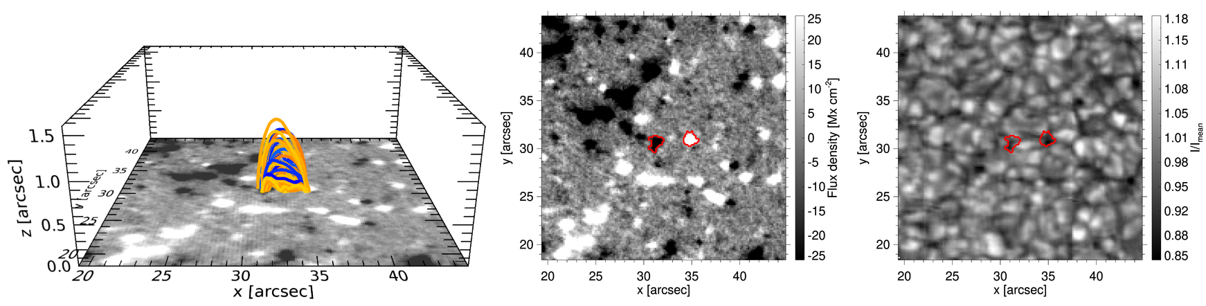
Figure 4: Example of an identified magnetic bipole. The left panel shows magnetic field lines connecting the footpoints of the bipole as derived from the magnetofrictional simulation. Different field lines have different colors for easier identification. The middle panel shows the loop footpoints (red contours) in the NFI magnetogram and the right panel the corresponding intensity filtergram. The observations were taken on November 3, 2010 at 01:34 UT. An animation showing the spatio-temporal evolution of the bipole is available in the online journal. The positive and negative polarity footpoints have lifetimes of $82.5$ min and $118.5$ min, respectively. Based on the magnetofrictional simulation, the footpoints are connected for about 40 minutes. The animation lasts 8 seconds and covers $\sim 2$ hours of solar time from November 3, 2010 at 01:17 UT.

The time-dependent bottom boundary conditions needed to drive the evolution of the magnetic field above the surface ($z>0$) are taken to be

$$-\frac{\partial A_{x}}{\partial t} = E_{x},$$ (6)

$$-\frac{\partial A_{y}}{\partial t} = E_{y},$$ (7)

where $E_{x}$ and $E_{y}$ are the horizontal components of the electric field vector, computed as $E_{x}=v_{y}B_{z}$ and $E_{y}=-v_{x}B_{z}$. Here, $v_{x}$ and $v_{y}$ represent the $x$ and $y$ components of the horizontal velocity field, respectively. We used Local Correlation Tracking (LCT; November & Simon, 1988) to determine $v_{x}$ and $v_{y}$ from the proper motion of the magnetic features. The LCT algorithm was applied to the NFI magnetogram sequence taking into account all the pixels. However, in the resulting horizontal velocity maps we set to zero the pixels with flux densities below 12 G ($3\sigma$). To avoid sharp changes in those pixels, we applied the smoothing function

$$f_{v}=1-\frac{1}{1+e^{B_{z}^{\prime}-12}}+\frac{1}{1+e^{B_{z}^{\prime}+12}},$$ (8)

where $B_{z}^{\prime}=B_{z}/1\mbox{G}$. An example of a horizontal velocity map is presented in Figure 2. Estimating the electric field in this way does not, in general, give a pair $(E_{x},E_{y})$ whose curl is equal to $-\partial B_{z}/\partial t$. Because of this, we use the method presented in Cheung & DeRosa (2012) to additionally solve for a correcting electric field to ensure the boundary $B_{z}$ is consistent with the NFI magnetogram sequence. To estimate the electric field, one could also use the method described in Kazachenko et al. (2014; see also Fisher et al. 2015, Lumme et al. 2017, Price et al. 2019, Hoeksema et al. 2020), but that would require vector magnetograms which are not available here.

The computation was performed in a box of size $L_{x}\times L_{y}\times L_{z}=61\times 64\times 21$ arcsec³. This box extends sufficiently high into the solar atmosphere to prevent the upper boundary from influencing the results in the photosphere and the lower chromosphere. Open boundary conditions were imposed at the top of the computational box.

4 Results

4.1 Magnetofrictional simulation

A 3D rendering of the magnetic field lines resulting from the magnetofrictional simulation of our data set is presented in Figure 3. The different colors of the field lines indicate the cosine of the field inclination to the local vertical, from $+1$ (positive polarity, violet) to $-1$ (negative polarity, red). To our knowledge, this is the first magnetofrictional simulation ever of a QS region including a full supergranular cell. One can clearly see small-scale, low-lying magnetic loops connecting patches of opposite polarity, and open field lines associated with unipolar patches (the mostly vertical red lines of negative polarity going away from the depicted volume through the upper plane). The magnetic topology of the region, together with its temporal evolution, holds the key to separate bipolar features from unipolar features.

It is important to mention here that the magnetofrictional simulation was tested for different FOV sizes. This was achieved by selecting different sizes of the Hinode/NFI FOV, as well as embedding the Hinode/NFI magnetograms into larger HMI magnetograms ($100\arcsec\times 100\arcsec$). The tests consistently produced open field lines extending up from the network regions above the supergranular cells. The field lines inside the supergranule seemed to be unaffected in the tests. Based on these results, we are confident that the periodic boundaries do not affect the extrapolation of the field lines inside the observed supergranular cell and that the general magnetic morphology in the selected FOV is determined by the network structures.

Figure 5: Magnetic loops (left) and clusters (right) detected in a Hinode magnetogram taken on November 3, 2010 at 00:24:04 UT. Flux patches belonging to the same loops or clusters have the same contour colors. The magnetograms are saturated at $\pm 30$ Mx cm^-2. An animation of this figure is available in the online journal. It shows the spatio-temporal evolution of all detected loops and clusters. The animation lasts 96 seconds and covers $23.7$ hours of solar time from November 2, 2010 at 08:31 UT.

The quality of the results can be seen in the movie accompanying Figure 4, which shows an example of a magnetic bipole detected in our magnetograms. The footpoints of the bipole emerged at the edges of the same granule and separated from each other with time. Using the magnetofrictional simulation we calculated the field lines and confirmed that the two footpoints are magnetically connected. The movie displays the complete history of the footpoints. Eventually, they disappeared via fragmentation and cancellation processes.

We would like to remind the reader that the simulation is not sufficiently accurate for the weakest magnetic features whose signal is close to the noise level. Such cases represent $\sim 25$% of the detected loops but only $11$% of the total bipolar flux, which is mainly determined by large loops and clusters.

4.2 Tracking results

The tracking of magnetic features in the selected region resulted in $10661$ unique features, comprising $86732$ individual patches over the whole sequence. A total of 8266 features appeared in situ, 1102 and 1190 were formed by fragmentation of existing unipolar and bipolar features, respectively, and 103 were present in the first frame. The latter were excluded from the analysis because we do not know their complete histories.

We classified the features appearing in situ as footpoints of magnetic loops, cluster members, or unipolar features by considering all 6 aspects described in Sect. 3.2. We found that 652 features were loop footpoints and 1428 emerged in 155 clusters during 22 hours of observations. This corresponds to $\sim$$8$% and $\sim$$17$% of the total number of magnetic features that appeared in situ. The remaining 6186 features ($75$%) were unipolar.

Among all the features born in situ and by fragmentation, 31% can be classified as bipolar and 69% as unipolar. However, the number of flux patches associated with bipolar and unipolar features is not so different (40686 vs 46046, or 47% vs 53%). This is because bipolar features tend to live longer and therefore contribute more flux patches per feature than their unipolar counterparts.

In the animation accompanying Figure 5 we show all the magnetic loops (left panel) and clusters (right panel) detected in our Hinode/NFI magnetograms. Flux patches belonging to the same loops or clusters have the same colors. The red circles outline the area where we look for bipolar features. The animation shows 22 hours of observations during which we tracked magnetic bipoles and two hours more to completely cover their lifetimes.

4.3 Properties of unipolar and bipolar IN flux patches

Figure 6: Physical parameters of 46046 unipolar and 40686 bipolar IN patches detected in this study. The upper panels show the unsigned magnetic flux (left) and flux density (right) distributions, while the bottom panels show the effective diameter (left) and feature lifetime (right) distributions. The blue and red solid lines represent unipolar and bipolar flux patches, respectively. The bin sizes used are $4\times 10^{15}$ Mx (flux), 0.5 Mx cm^-2 (flux density), 0.1 arcsec (diameter), and 3 minutes (lifetime).

To characterize the detected unipolar and bipolar magnetic patches, we calculated their unsigned magnetic fluxes, magnetic flux densities, sizes, and lifetimes. We define the unsigned magnetic flux of an individual patch as

$${\Phi}=\sum_{i=1}^{N}|\phi_{i}|\,{\rm d}A,$$ (9)

where $N$ is the number of pixels in the patch, ${\rm d}A$ the area of a pixel, and $\phi_{i}$ the magnetic flux density observed in pixel $i$. We also compute the average magnetic flux density of the patch as

$$\overline{\phi}=\frac{1}{N}\sum_{i=1}^{N}\phi_{i}.$$ (10)

This quantity provides an estimate of the longitudinal magnetic field strength in the patch, assuming a filling factor equal to one.

The distributions of the various parameters are shown in Fig. 6 separately for unipolar and bipolar patches. The mean values over the two populations are given in Table 1.

As can be seen in the upper left panel of Figure 6, unipolar patches span three decades in flux, from our detection limit of $6.5\times 10^{15}$ Mx to about $3\times 10^{18}$ Mx, with a mean value of $9.2\times 10^{16}$ Mx. The flux of bipolar patches spans from the detection limit to approximately $5.4\times 10^{18}$ Mx. Their mean flux is $24.1\times 10^{16}$ Mx, more than a factor $2.6$ larger than that of unipolar patches.

The lowest value of the flux density distribution is $12$ Mx cm^-2 for both populations as a consequence of the $3\sigma$ threshold used to identify the patches. The largest flux densities are about $90$ Mx cm^-2 and $115$ Mx cm^-2 for unipolar and bipolar patches, respectively. The mean flux densities of unipolar and bipolar patches are $19.9$ Mx cm^-2 and $25.7$ Mx cm^-2, respectively. Therefore, bipolar patches tend to be stronger. The strongest flux concentrations correspond to those appearing in clusters.

Table 1 shows that bipolar patches are in nearly perfect flux balance, with positive patches accounting for 51% of the total bipolar flux observed in the cell. By contrast, unipolar patches exhibit a certain amount of flux imbalance: about 62% of the total unipolar flux is negative due to the surplus of negative patches that is detected. Interestingly, also the supergranular cell is dominated by negative polarity fields. For this reason, the possibility exists that a fraction of the negative unipolar patches are actually formed by accumulation of background flux from the supergranule itself and not by a more flux-balanced mechanism.

The mean effective diameter is about $0.8$ arcsec for unipolar patches and about $1.1$ arcsec for bipolar patches. Here the effective diameter is defined as that of a circular structure with the same area as the identified magnetic patch. The largest unipolar and bipolar patches in our data set have effective diameters of $3.3$ and $5.4$ arcsec, respectively. Thus, most bipolar patches are bigger than unipolar patches, although some of them can be very small too.

Table 1: Physical parameters of the detected unipolar and bipolar IN patches

	Unipolar	Bipolar
Total number of features	7288	3270
Total number of patches	46046	40686
Number of positive patches	19486	19173
Number of negative patches	26560	21513
Mean unsigned flux [$10^{16}$ Mx]	9.2	24.1
positive patches [$10^{16}$ Mx]	8.3	25.9
negative patches [$10^{16}$ Mx]	9.9	22.4
Total unsigned flux carried by
positive patches [$10^{21}$ Mx]	1.6	5.0
negative patches [$10^{21}$ Mx]	$2.6$	4.8
Mean flux density [Mx cm-2]	19.9	25.7
Mean effective diameter [arcsec]	0.8	1.1
Mean lifetime [min]	10.7	23.4

Similarly to Gošić et al. (2014, 2016), we consider a feature to live from the frame in which it receives a unique label until the moment it loses its label. In our magnetogram sequence, the lifetimes range from 1.5 min up to $\sim 330$ min (unipolar features) and $\sim 345$ min (bipolar features). The lower limit is set by the detection threshold. On average, bipolar features live significantly longer than unipolar features ($23.4$ vs $10.7$ min). This is because they tend to be larger, so they have a better chance to survive interactions with other magnetic features and require more time to disperse. If we consider bipolar loops and clusters to live from the moment when the first footpoint or member appears until all of them disappear, then their average lifetime is even longer ($62$ min).

Magnetic features that have long lifetimes usually appear in clusters. They undergo multiple mergings which help them accumulate enough flux to withstand convective dragging, fragmentation and partial cancellation over longer periods of time. The red arrow in Figure 5 indicates one such feature. However, long lifetimes are not only associated with bipolar features. Although less common, unipolar features can also live for 4-5 hours when they find themselves in the right environment, i.e., when they are surrounded mostly by same-polarity features and have enough time for merging processes to occur multiple times.

Long-lived features are strong magnetic flux concentrations and may have a substantial impact on the QS chromosphere. This could be realized, for example, through reconnection between the preexisting ambient fields and the IN flux concentrations emerging into the chromosphere (Gošić et al., 2021). It is also possible that the long-lived IN features may affect the chromospheric velocity field and the low-lying canopy that extends above supergranular cells (Robustini et al., 2019).

Figure 7: Location of appearance of bipolar (left) and unipolar (right) features inside the supergranular cell. Green dots represent flux features emerging in clusters while the footpoints of magnetic loops are shown with red dots. Blue dots mark where unipolar features appear. The background image is the mean magnetogram averaged over the 22 hours duration of the time sequence.

Figure 8: Temporal evolution of the total instantaneous unsigned flux carried by the unipolar (blue) and bipolar (red) features that originated within the selected circular region, along with their sum (black). The dotted lines mark the period without reliable data due to the existence of features at the beginning of the sequence whose modes of appearance are not known.

Figure 9: Fraction of the total instantaneous unsigned flux within the selected supergranular region in the form of bipolar features. The green and red lines correspond to clusters and loops, respectively, while the orange line shows their sum. The dotted lines mark incomplete data at the beginning of the sequence.

4.4 Spatial distribution

Our observations reveal that bipolar features emerge everywhere in the selected region. In Figure 7 we plot the locations of appearance of all bipolar and unipolar features. As can be seen, loops and clusters are more or less uniformly distributed inside the circle and do not show any preferred emergence location after 22 hours of observations. Unipolar features also appear uniformly across the supergranule. We would like to remind the reader that the appearance locations represent the flux-weighted centers of the magnetic patches at birth. Therefore, the actual area occupied by them is larger and covers the entire cell. Indeed, over a period of 22 h we do not see any dead calm area of the type detected by Martínez González et al. (2012) in SUNRISE/IMaX magnetogram sequences of about 30 min duration.

4.5 Unipolar and bipolar flux budget

Figure 10: Appearance rates of bipolar and unipolar flux in the IN. The red lines shows the flux brought to the surface by magnetic loops and clusters at birth and during their evolution, while the blue line represents unipolar features. The total appearance rate is shown in black. To improve the statistics, bins of $0.5$ h are used.

The total instantaneous unsigned fluxes of unipolar and bipolar IN features are shown in Figure 8 (blue and red curves, respectively). The first three hours are not reliable since we do not know the modes of appearance of the features that were visible in the first frame. It was necessary to wait 3 h for all those features to disappear. We can see here that the flux carried by unipolar features is practically constant with time. On the other hand, the flux brought by loops and clusters shows strong variations, especially when large clusters emerge. Bipolar features experience an intrinsic growth in flux and size over their lifetime, and this partly explains the positive excursions associated with the appearance of clusters. Moreover, the two curves are affected by interactions between features, which mix the unipolar and bipolar fluxes. For example, when a small unipolar feature merges with a strong feature from a cluster and cannot be tracked any longer, the flux of the smaller feature is added to the flux of the cluster, i.e., the total bipolar flux increases at the expense of the unipolar flux. However, this is balanced to some extent as the same process happens in the opposite direction as well. Finally, the curves are also affected by mergings and cancellations of IN patches with NE elements, which cause drops in the total amount of flux (stronger for bipolar features, as they tend to be bigger and carry more flux per feature).

The contribution of bipolar features to the total instantaneous flux of this supergranular cell is very significant, as can be seen in Figure 9. After the initial three hours, the flux carried by clusters represents about $60$% of the total detected flux, while the loops contain $12$% of the detected flux. Together, clusters and loops account for $\sim$$72$% of the IN flux, with temporal variations from $50$% to $95$%. The rest of the flux in this supergranular cell is in the form of unipolar features. Interestingly, close to the end of the sequence there is a 30-minute interval when the bipolar flux accounts for only $\sim$$20$% of the total flux. This period coincides with a lack of large bipolar features.

4.6 Unipolar and bipolar flux appearance rate

Figure 10 shows the flux appearance rate of bipolar (loops and clusters) and unipolar features as a function of time. The data have been binned over 30 minutes. Each bin represents the sum of the flux brought to the surface by new features and the flux gained by already existing features during that period of time (for more details, see Gošić et al. 2016). The total flux appearance rate in the central part of the supergranular cell is $123$ Mx cm^-2 day^-1, in agreement with the value reported by Gošić et al. (2016). Bipolar flux emerges on the surface at a rate of $68$ Mx cm^-2 day^-1, or 55% of the total rate. The remaining $55$ Mx cm^-2 day^-1 (45% of the total rate) is due to unipolar features.

In Figure 10, all the curves show temporal variations. In the case of loops and clusters, the variations are larger when strong bipolar features emerge, for example around 9, 11 and 16 h. Unipolar fields are more stable: their appearance rates are almost constant in the first $8$ hours and in the last 6 hours. However, they fluctuate when clusters emerge. It may happen that in such periods we detect fewer unipolar patches because the strong bipolar patches occupy a larger surface area. The appearance rate of bipolar flux in the first three hours is most likely underestimated, explaining why it is so low. The reason is that we cannot classify as unipolar or bipolar the magnetic features that were visible in the first frame. These features and their fragments were discarded from the analysis during the first three hours (the time they needed to completely leave the selected region), so any flux gain they might have experienced during that time was not counted. This primarily affects large magnetic features such as those that normally emerge in bipolar form. In any case, the black curve shows that the total flux appearance rate was normal during the first three hours, even if this is not reflected in the other curves.

Finally, we should keep in mind that unipolar features in our data set are smaller and contain less flux than bipolar features. Many of them have signals that fluctuate around the threshold level. Because of this, they may disappear and reappear frequently in the magnetograms. Thus, even though we correct for reappearing events as in Gošić et al. (2016), unipolar features do not necessarily represent new flux brought to the surface. For that reason, their appearance rate should be considered as an upper limit.

5 Discussion and Conclusions

In this paper, we studied the appearance modes and the temporal evolution of IN magnetic features inside a supergranular cell. We used a high-resolution, high-sensitivity, long-duration Hinode/NFI magnetogram sequence taken on 2010 November 2–3. We tracked flux features inside the supergranule and for the first time we employed magnetofrictional simulations to identify unipolar and bipolar features in the cell interior. We then determined how and where these fields appear and calculated the total unsigned flux they bring to the surface. Our findings can be summarized as follows:

1. Bipolar features (magnetic loops and flux clusters) appear more or less uniformly inside the supergranular cell. This is at odds with Martínez González et al. (2012) and Stangalini (2014). Perhaps the reason is the shorter duration of the time sequences they used, which may have resulted in insufficient statistics (particularly for clusters). In our data set, on supergranular time scales all the observed area eventually undergoes emergence processes. Thus, the magnetic voids reported in the literature are short-lived patterns (existing on granular/mesogranular time scales only) or do not occur in the cell we have studied. It is important to mention that there are indeed periods where less magnetic flux is brought to the solar surface, which can be easily identified in Figures 1, 8, 9, and 10. However, even during those periods magnetic patches appear evenly distributed across the supergranule, as can be seen in Figure 5.13 of Gošić (2012).

2. Bipolar features emerge in the interior of the supergranular cell at a rate of 68 Mx cm^-2 day^-1. This is new IN flux coming most likely from below the surface. It accounts for 55% of the total flux appearance rate.

3. Unipolar features appear at a rate of 55 Mx cm^-2 day^-1, or 45% of the total flux appearance rate.

4. On average, bipolar features contain about 72% of the total instantaneous IN flux. This value is observed to fluctuate between 50% and 95% with time. It drops to 20% for only about 30 minutes close to the end of the sequence. The fraction of bipolar instantaneous flux is larger than the bipolar flux appearance rate due to two processes: the intrinsic growth of bipolar features in flux and size during the early phases of emergence, and the transfer of flux that happens when (usually small) unipolar features merge with bipolar features and disappear as individual elements.

Our results lend support to the idea that there are two distinct populations of IN flux concentrations inside supergranular cells. One group consists of unipolar features while the second group are bipolar features. Unipolar flux concentrations are probably formed by coalescence of background flux, as pointed out by Lamb et al. (2008) and also suggested by the analysis presented by Gošić et al. (2016).

Figure 11: Orientation of the magnetic axes of bipolar features emerging in the IN with respect to solar East-West. The axis is defined as the vector connecting the negative and positive footpoints of loops (red) or the flux-weighted centers of negative and positive flux patches in clusters (green). The angles increase counterclockwise. An angle of $0^{\rm o}$ represents a magnetic bipole parallel to the solar equator, pointing West. The data are binned in $30^{\circ}$ intervals.

Bipolar features may be the signature of local dynamo action or a result of the global dynamo. The second possibility is perhaps less probable, given that the two footpoints of the loops and the opposite-polarity centers of the clusters do not seem to show a systematic orientation upon appearance. This is illustrated in Figure 11. Thus, either they are not oriented in any preferred direction (favoring the local dynamo scenario) or the orientation they adopt is largely determined by convective flows during the emergence process (not by the orientation they have deep in the convection zone).

The results presented in this work partially agree with those based on SUNRISE/IMaX data (Anusha et al., 2017; Smitha et al., 2017). We confirm the IMaX result that unipolar features are more numerous than bipolar features. However, in our magnetograms bipolar features account for 55% of the flux appearance rate, as opposed to only $\sim$9% in the IMaX data (Smitha et al., 2017). We should keep in mind that the IMaX observations have shorter duration than the NFI sequence used here, i.e., they cover only a very small fraction of the typical supergranular time scales. Statistical fluctuations cannot be ruled out in this case. In particular, it is likely that IMaX did not capture clusters and/or large magnetic loops, which would significantly decrease the contribution of bipolar features to the flux appearance rate. Also, the particular ability of the tracking algorithms to recognize magnetic elements as unipolar or bipolar features may have caused additional differences among the reported rates.

Another source of discrepancy is the total flux appearance rate itself. The values inferred by Smitha et al. (2017) are an order of magnitude larger than ours. The difference may be due to the higher sensitivity and spatial resolution of the IMaX observations, together with the use of a lower detection threshold ($2\sigma$ vs $3\sigma$) and no minimum lifetime for features to be included in the analysis. This led to the detection of much weaker flux features in the IMaX magnetograms as compared with the NFI observations ($9\times 10^{14}$ Mx vs $5\times 10^{15}$ Mx) and many more features per frame, which may well explain the different total flux appearance rates. Finally, one should not forget that the spectral lines observed by Hinode and IMaX are different – they have different magnetic sensitivities and sample different atmospheric layers. The Hinode/NFI line is formed in the mid/upper photosphere and therefore can be expected to yield fewer features (because most of them lie in the lower photosphere) and weaker fluxes (due to the general reduction of the magnetic field with height). This might also partially explain the different results obtained from Hinode/NFI and SUNRISE/IMaX.

To better understand the magnetism of the QS, we need to investigate how different methods and instruments may affect the analysis of the flux appearance modes in the QS. However, it is also clear that we will need measurements at higher resolution and sensitivity to capture the weakest magnetic fields of the solar internetwork. This will soon be made possible by a new generation of telescopes, particularly the Daniel K. Inouye Solar Telescope (Rimmele et al., 2020).

References

- Anusha et al. (2017) Anusha, L. S., Solanki, S. K., Hirzberger, J., & Feller, A. 2017, A&A, 598, A47
- Barthol et al. (2011) Barthol, P., Gandorfer, A., Solanki, S. K., et al. 2011, Sol. Phys., 268, 1
- Cattaneo (1999) Cattaneo, F. 1999, ApJ, 515, L39
- Cattaneo & Hughes (2001) Cattaneo, F., & Hughes, D. W. 2001, Astron. Geophys., 42, 18
- Centeno et al. (2007) Centeno, R., Socas-Navarro, H., Lites, B., et al. 2007, ApJ, 666, 137
- Chae (2001) Chae, J. 2001, ApJ, 560, L95
- Cheung & DeRosa (2012) Cheung, M. C. M., & DeRosa, M. L. 2012, ApJ, 757, 147
- Cheung et al. (2015) Cheung, M. C. M., De Pontieu, B., Tarbell, T. D., et al. 2015, ApJ, 801, 83
- Craig & Sneyd (1986) Craig, I. J. D., & Sneyd, A. D. 1986, ApJ, 311, 451
- Danilovic et al. (2010a) Danilovic, S., Schüssler, M., and Solanki, S. K. 2010, A&A, 513, A1
- Danilovic et al. (2010b) Danilovic, S., Beeck, B., Pietarila, A., et al. 2010, ApJ, 723, L149
- de Wijn et al. (2005) de Wijn, A. G., Rutten, R. J., Haverkamp, E. M. W. P., and Sütterlin, P. 2005, A&A, 441, 1183
- de Wijn et al. (2009) de Wijn, A.G., Stenflo, J.O., Solanki, S.K., and Tsuneta, S. 2009, Space Sci. Rev., 144, 275
- Fischer et al. (2020) Fischer, C. E., Vigeesh, G., Lindner, P., et al. 2020, ApJ, 903, L10
- Fisher et al. (2015) Fisher, G. H., Abbett, W. P., Bercik, D. J., et al. 2015, SpWea, 13, 369
- Giannattasio et al. (2020) Giannattasio, F., Consolini, G., Berrilli, F., & Del Moro, D. 2020, ApJ, 904, 7
- Gošić (2012) Gošić, M. 2012, Master Thesis, University of Granada (Spain)
- Gošić et al. (2014) Gošić, M., Bellot Rubio, L.R., Orozco Suárez, D., Katsukawa, Y., and del Toro Iniesta, J.C. 2014, ApJ, 797, 49
- Gošić et al. (2016) Gošić, M., Bellot Rubio, L.R., del Toro Iniesta, J.C., Orozco Suárez, D., and Katsukawa, Y. 2016, ApJ, 820, 35
- Gošić et al. (2021) Gošić, M., De Pontieu, B., Bellot Rubio, L. R., et al. 2021, ApJ, 911, 41
- Gömöry et al. (2010) Gömöry, P., Beck, C., Balthasar, H., et al. 2010, A&A, 511, A14
- Guglielmino et al. (2012) Guglielmino, S. L., Martínez Pillet, V., Bonet, J. A., et al. 2012, ApJ, 745, 160
- Hagenaar (2001) Hagenaar, H. J. 2001, ApJ, 555, 448
- Harvey & Martin (1973) Harvey, K. L., and Martin, S. F. 1973, Sol. Phys., 32, 389
- Harvey et al. (1975) Harvey, K. L., Harvey, J. W., and Martin, S. F. 1975, Sol. Phys., 40, 87
- Hoeksema et al. (2020) Hoeksema, J. T., Abbett, W. P., Bercik, D. J. 2020, ApJS, 250, 28
- Kazachenko et al. (2014) Kazachenko, M. D., Fisher, G. H., & Welsch, B. T. 2014, ApJ, 795, 17
- Kosugi et al. (2007) Kosugi, T., Matsuzaki, K., Sakao, T., et al. 2007, Sol. Phys., 243, 3
- Lamb et al. (2008) Lamb, D. A., DeForest, C. E., & Hagenaar, H., J. et al. 2008, ApJ, 674, 520
- Lamb et al. (2010) Lamb, D. A., DeForest, C. E., & Hagenaar, H., J. et al. 2010, ApJ, 720, 1405
- Li et al. (2019) Li, S., Jaroszynski, S., Pearse, S., Orf, L. & Clyne, J. 2019, Atmosphere, 10, 488
- Livingston & Harvey (1971) Livingston, W., & Harvey, J. 1971, in Solar Magnetic Fields, ed. R. Howard (Dordrecht: Reidel), IAU Symp., 43, 51
- Livingston & Harvey (1975) Livingston, W. C., & Harvey, J. 1975, BAAS, 7, 346
- Lites (2002) Lites, B. W. 2002, ApJ, 573, 431
- Lumme et al. (2017) Lumme, E., Pomoell, J. & Kilpua, E. K. J. 2017, Sol. Phys., 292, 191
- Martin (1988) Martin, S. F. 1988, Sol. Phys., 117, 243
- Martin (1990) Martin, S. F. 1990, in IAU Symp. 138, Solar Photosphere: Structure, Convection, and Magnetic Fields, ed. J. O. Stenflo (Cambridge: Cambridge Univ. Press), 138, 129
- Martínez González et al. (2007) Martínez González, M. J., Collados, M., Ruiz Cobo, B., & Solanki, S. K., et al. 2007, A&A, 469, L39
- Martínez González & Bellot Rubio (2009) Martínez González, M. J., & Bellot Rubio, L. R. 2009, ApJ, 700, 1391
- Martínez González et al. (2012) Martínez González, M. J., Manso Sainz, R., Asensio Ramos, A., & Hijano, E. 2012, ApJ, 755, 175
- Martínez Pillet et al. (2011) Martínez Pillet, V., Del Toro Iniesta, J. C., Álvarez-Herrero, A., et al. 2011, Sol. Phys., 268, 57
- Meunier et al. (1998) Meunier, N., Solanki, S. K., & Livingston, W. C. 1998, A&A, 331, 771
- November & Simon (1988) November, N., & Simon, W. G. 1998, ApJ, 333, 427
- Orozco Suárez et al. (2008) Orozco Suárez, D., Bellot Rubio, L. R., & Cheung, M. C. M. et al. 2008, A&A, 481, L33
- Parnell et al. (2009) Parnell, C. E., DeForest, C. E., & Hagenaar, H. J. et al. 2009, ApJ, 698, 75
- Palacios et al. (2012) Palacios, J., Blanco Rodríguez, J., Vargas, S. et al. 2012, A&A, 537, 21
- Pietarila Graham et al. (2010) Pietarila Graham, J., Cameron, R. H., & Schüssler, M. 2010, ApJ, 714, 1606
- Pietarila Graham et al. (2011) Pietarila A., Cameron, R. H., Danilovic, S., et al. 2011, ApJ, 729, 136
- Ploner et al. (2001) Ploner, S. R. O., Schüssler, M., Solanki, S. K., and Gadun, A. S. 2001, ASP Conference Series, 236, 363
- Price et al. (2019) Price, D. J., Pomoell, J., Lumme, E., & Kilpua, E. K. J. 2019, A&A, 628, 114
- Rempel (2014) Rempel, M. 2014, ApJ, 789, 132
- Rempel (2018) Rempel, M. 2018, ApJ, 859, 161
- Rimmele et al. (2020) Rimmele, T. R., Warner, M., Keil, S. L., et al. 2020, Sol. Phys., 295, 172
- Robustini et al. (2019) Robustini, C., Esteban Pozuelo, S., Leenaarts, J., de la Cruz Rodríguez, J. 2019, A&A, 621, 1
- Scherrer et al. (1995) Scherrer, P. H., Bogart, R. S., & Bush, R. I. et al. 1995, Sol. Phys., 162, 129
- Schrijver & Harvey (1994) Schrijver, C. J., & Harvey, K. L. 1994, Sol. Phys., 150, 1
- Schrijver & van Ballegooijen (2005) Schrijver, C.J., & van Ballegooijen, A.A. 2005 ApJ, 630, 552
- Sheeley (1969) Sheeley, N. R. Jr. 1969, Sol. Phys., 9, 347
- Smitha et al. (2017) Smitha, H. N., Anusha, L. S., Solanki, S. K., & Riethmüller, T. L. 2017, ApJ, 229, 17
- Smithson (1975) Smithson, R. C. 1975, BAAS, 7, 346
- Solanki et al. (2010) Solanki, S. K., Barthol, P., Danilović, S., et al. 2010, ApJ, 723, L127
- Stangalini (2014) Stangalini, M. 2014, A&A, 561, L6
- Straus et al. (1992) Straus, T., Deubner, F.-L., & Fleck, B. 1992, A&A, 256, 652
- Title et al. (1989) Title, A. M., Tarbell, T. D., Topka, K. P., et al. 1989, ApJ, 336, 475
- Trujillo Bueno et al. (2004) Trujillo Bueno, J., Shchukina, N., & Asensio Ramos, A. 2004, Nature, 430, 326
- Tsuneta et al. (2008) Tsuneta, S., Ichimoto, K., & Katsukawa, Y. 2008, Sol. Phys., 249, 167
- Vögler & Schüssler (2007) Vögler, A., & Schüssler, M. 2007, A&A, 465, L43
- Wang et al. (1995) Wang, J., Wang, H., Tang, F., et al. 1995, Sol. Phys., 160, 277
- Welsch & Longcope (2003) Welsch, B. T., & Longcope, D. W. 2003, ApJ, 588, 620
- Woodard & Chae (1999) Woodard, M.F., Chae, J.C. 1999, Sol. Phys., 184, 239
- Yang et al. (1986) Yang, W. H., Sturrock, P. A., & Antiochos, S. K. 1986, ApJ, 309, 383
- Zhao et al. (2009) Zhao, M., Wang, J.X., Jing, C.L., Zhou, G.P. 2009, Chin. J. Res. Astron. Astrophys. 9, 933
- Zhou et al. (2013) Zhou, G., Wang, J., & Jin, C. 2013, Sol. Phys., 283, 273