On the evolution of inhomogeneous perturbations
in the $\Lambda$CDM model and $f\left(R\right)$ modified gravity theories

Abstract

We focus on weak inhomogeneous models of the Universe at low redshifts, described by the Lemaître-Tolman-Bondi (LTB) metric. The principal aim of this work is to compare the evolution of inhomogeneous perturbations in the $\Lambda$CDM cosmological model and $f(R)$ modified gravity theories, considering a flat Friedmann-Lemaître-Robertson-Walker (FLRW) metric for the background. More specifically, we adopt the equivalent scalar-tensor formalism in the Jordan frame, in which the extra degree of freedom of the $f(R)$ function is converted into a non-minimally coupled scalar field. We investigate the evolution of local inhomogeneities in time and space separately, following a linear perturbation approach. Then, we obtain spherically symmetric solutions in both cosmological models. Our results allow us to distinguish between the presence of a cosmological constant and modified gravity scenarios, since a peculiar Yukawa-like solution for radial perturbations occurs in the Jordan frame. Furthermore, the radial profile of perturbations does not depend on a particular choice of the $f(R)$ function, hence our results are valid for any $f(R)$ model.

Introduction

The well-known $\Lambda$CDM model [1, 2], which includes a cosmological constant $\Lambda$ and a cold dark matter (CDM) component, is based on General Relativity (GR), and it provides a robust and accurate description of our Universe, supported by cosmological data. Moreover, the Universe appears homogeneous and isotropic at very large scales [3] (cosmological principle), and this kind of geometry is described by the FLRW line element. In this work, based on a paper in preparation [4], we investigate possible deviations from two pillars of the standard $\Lambda$CDM model, focusing on a local inhomogeneous description of the Universe and modified gravity models.

Here, we adopt the LTB metric [2], a spherically symmetric solution of the Einstein field equations, to account for local deviations of the Universe from the homogeneity. Hence, we regard the weakly inhomogeneous LTB solution as the standard FLRW geometry plus small spherically symmetric perturbations.

Furthermore, in recent years increasing interest raised to provide features able to distinguish between GR and modified gravity approaches. Some open problems in cosmology, such as the Hubble constant tension [5], may require new physics [6]. The aim of the present work is to compare the evolution of linear inhomogeneous perturbations in the $\Lambda$CDM and $f\left(R\right)$ modified gravity models [7, 8]. More in detail, we used the equivalent formalism in the Jordan frame [7, 8, 9], and we adopt the $f\left(R\right)$ Hu-Sawicki model [10], which is a promising theoretical framework to reproduce the cosmic acceleration in the late Universe via the dynamics of a non-minimally coupled scalar field without a cosmological constant.

Then, we investigate the dynamics of inhomogeneous perturbations in the two cosmological models abovementioned. Moreover, the separable variables method is implemented in the analysis at the first-order of perturbation, and our approach is the same used in Ref. 11. We obtain an analytic expression only for the radial dependence of linear perturbations, while their time evolution must be numerically evaluated. The most relevant issue, emerging from our analysis, is the different morphology of the radial dependence of the LTB solution in the $\Lambda$CDM formulation and Hu-Sawicki dynamics. Indeed, a distinctive Yukawa-like behavior occurs in the Jordan frame gravity regardless of the choice of a specific $f\left(R\right)$ model. Hence, we have found a peculiar feature to distinguish a modified gravity model from a cosmological constant scenario.

This work is organized as follows: in Sec. 1 we introduce the framework of the $f\left(R\right)$ extended gravity models; in Sec. 2 we adopt the LTB metric; then, in Sec. 3 we implement a perturbation approach to deal with local inhomogeneities. Finally, we summarize our work in Sec. 4. We adopt the metric signature $\left(-,+,+,+\right)$, and we set $c=1$.

1 $f\left(R\right)$ models in the Jordan frame

A generalization of the Einstein-Hilbert theory is provided by the so-called $f\left(R\right)$ modified gravity models [7, 8]. In this context, the gravitational Lagrangian density is expressed as a free function $f$ of the Ricci scalar $R$, namely an extra degree of freedom compared to GR. The extended field equations in $f\left(R\right)$ gravity are fourth-order partial differential equations in the metric tensor components. In particular, if $f\left(R\right)=R$, the gravitational field equations end up in the Einstein equations in GR, trivially.

It is often convenient to reformulate $f\left(R\right)$ gravity in the scalar-tensor representation in the Jordan frame [7, 8, 9]. In doing so, the extra degree of freedom of the $f\left(R\right)$ function is converted into a non-minimally coupled scalar field. It can be checked that the following action

$$S_{J}=\frac{1}{2\,\chi}\,\int_{\Omega}d^{4}x\,\sqrt{-g}\,\left[\phi\,R-V\left(\phi\right)\right]+S_{M}\left(g_{\mu\nu},\psi\right)$$ (1)

is dynamically equivalent to the action in the $f\left(R\right)$ metric formalism, if $f^{\prime\prime}\left(R\right)\neq 0$, where we have defined a scalar field $\phi=f^{\prime}\left(R\right)=df/dR,$ and a scalar field potential $V\left(\phi\right)=\phi\,R\left(\phi\right)-f\left(R\left(\phi\right)\right)$. In Eq. (1), $\chi\equiv 8\,\pi\,G$ is the Einstein constant, $G$ is the Newton constant, $g$ is the determinant of the metric tensor $g_{\mu\nu}$, while $S_{M}$ is the matter action, and $\psi$ denotes matter fields. The advantage of the Jordan frame is that the corresponding field equations [8] are now second-order differential equations, but one has to deal with the non-minimally coupling.

The increasing attention to these extended gravity models is motivated by the consideration that the actual cosmic acceleration of the Universe might be obtained by geometry rather than a cosmological constant. A geometrical modification, indeed, could be regarded as an effective matter source.

Among several suggested $f\left(R\right)$ models [7, 8, 12, 13], we focus on the Hu-Sawicki proposal [10], which is largely studied in the late Universe. The deviation $F\left(R\right)\equiv f\left(R\right)-R$ with respect to the GR scenario for the Hu-Sawicki (HS) model with $n=1$ assumes the following form

$$F\left(R\right)=-m^{2}\frac{c_{1}\,R/m^{2}}{c_{2}\,R/m^{2}+1}\,,$$ (2)

where $m^{2}\equiv\frac{\chi\,\rho_{m0}}{3}$ is related to the present matter density $\rho_{m0}$, while $c_{1}$ and $c_{2}$ are dimensionless parameters. It can be checked [10] that an effective cosmological constant is obtained for $R\gg m^{2}$. Furthermore, $c_{1}$ and $c_{2}$ can be constrained [10] specifying $F_{R0}\equiv dF\,/\,dR\,\left(z=0\right)$ at the present cosmic time (redshift $z=0$).

Finally, we write the scalar field potential $V\left(\phi\right)$ in the Jordan frame for the HS model with $n=1$:

$$V\left(\phi\right)=\frac{m^{2}}{c_{2}}\,\left[c_{1}+1-\phi-2\sqrt{c_{1}\,\left(1-\phi\right)}\right]\,.$$ (3)

It can be shown [14] that the potential (3) ends in an asymptotically stable de Sitter Universe.

2 Inhomogeneous solutions in GR and in the Jordan frame

An inhomogeneous Universe can be described by using the LTB line element [2], which is a spherically symmetric solution of the Einstein equations. The Universe in the LTB geometry appears inhomogeneous, but isotropic, from a single preferred point located at the center of the spherical symmetry. For instance, a cosmological dust or a spherical overdensity mass are well described by such a metric.

In the synchronous gauge, the LTB line element may be regarded as a generalization of the FLRW one, and it is given by

$$ds^{2}=-dt^{2}+e^{2\alpha}dr^{2}+e^{2\beta}\,\left(d\theta^{2}+sin^{2}\theta\,d\phi^{2}\right)\,,$$ (4)

where $r$ is the radial distance from the preferred point, while $\alpha=\alpha\left(t,\,r\right)$ and $\beta=\beta\left(t,\,r\right)$ are two metric functions.

Considering a pressure-less dust ($p=0$) and a cosmological constant $\Lambda$ in GR, we can write the Einstein equations in the LTB metric. For instance, the 01 component of field equations is written as

$$\frac{\dot{\beta}^{\prime}}{\beta^{\prime}}-\dot{\alpha}+\dot{\beta}=0$$ (5)

where $\dot{\left(\right)}$ and $\left(\right){}^{\prime}$ denote derivatives with respect to time $t$ and radial coordinate $r$, respectively. The other non-zero equations are the 00 and 11 components [4], while different components vanish due to spherical symmetry.

It is possible to simplify the LTB metric within the framework of GR, using Eq. (5), which allows us to find a relation between the metric functions $\alpha$ and $\beta$. Following the approach in Ref. 2, the LTB line element (4) becomes

$$ds^{2}=-dt^{2}+\frac{\left[\left(a\,r\right){}^{\prime}\right]{}^{2}}{1-r^{2}\,K^{2}}dr^{2}+\left(a\,r\right){}^{2}\,\left(d\theta^{2}+sin^{2}\theta\,d\phi^{2}\right)\,,$$ (6)

where $a=a\left(t,r\right)=e^{\beta}/r$ is a generalized scale factor in a inhomogeneous geometry, and $K=K\left(r\right)$. Note that if $a\left(t,r\right)$ and $K\left(r\right)$ are independent of $r$, the metric (6) coincides with the FLRW line element, describing an isotropic and homogeneous geometry. Moreover, the 00 and 11 components of the Einstein equations in the LTB metric provides a generalization of the Friedmann equations in the $\Lambda$CDM model.

Concerning the $f\left(R\right)$ modified gravity scenario in the equivalent Jordan frame, the 01 component of the gravitational field equations in the LTB metric is written as

$$\frac{\dot{\beta}^{\prime}}{\beta^{\prime}}-\dot{\alpha}+\dot{\beta}=-\frac{1}{2\,\phi\,\beta^{\prime}}\,\left(\dot{\phi}^{\prime}-\dot{\alpha}\,\phi^{\prime}\right)\,.$$ (7)

Furthermore, we can compute [4] also the 00 and 11 of field equations, as well as the scalar field equation in the Jordan frame. Observe that $\phi$, $\rho$, $\alpha$, and $\beta$ are all functions of $t$ and $r$ in a inhomogeneous scenario.

Comparing Eq. (7) with the respective equation (5) obtained in GR, an extra term occurs in the Jordan frame due to non-minimal coupling between $\phi$ and the metric functions $\alpha$, $\beta$. As a consequence, we can not relate $\alpha$ and $\beta$ to rewrite the LTB metric as in the GR scenario. Moreover, the scalar field potential $V\left(\phi\right)$ does not affect Eq. (7), but it is included in the remaining field equations. $V\left(\phi\right)$ represents an extra degree of freedom with respect to GR, and the dynamics in the Jordan frame deviates from that of the Einstein theory.

3 Perturbation approach in GR and in the Jordan frame

In this Section, we investigate the different evolution of local inhomogeneities within the framework of GR and modified gravity [4]. Here, we stress one important difference: we can not adopt the LTB metric in the form (6) in the Jordan frame, but we have to refer to the line element in Eq. (4), as motivated in Sec. 2.

Then, we consider the LTB metric to describe local inhomogeneities as small linear perturbations with respect to a flat FLRW metric as background. Hence, we can write all the physical quantities as a background term, denoted with a bar, plus a linear perturbation, which depends on $t$ and $r$, and it is denoted with $\delta$. For instance, the energy density is written as $\rho\left(t,r\right)=\bar{\rho}\left(t\right)+\delta\rho\left(t,r\right)\,.$ Similarly, we rewrite the scale factor $a\left(t,r\right)$ in GR, the scalar field $\phi\left(t,r\right)$, the metric functions $\alpha\left(t,r\right)$, and $\beta\left(t,r\right)$ in the Jordan frame. We also assume that perturbation terms are small corrections if compared with respective background quantities, i.e. $\delta\rho\ll\bar{\rho}$. Furthermore, we consider $K^{2}\left(r\right)$ in the LTB metric (6) as a linear term, since it is related to inhomogeneities. It should be noted that, comparing the LTB line element (4) and a flat FLRW metric, we have to require two constraints: $\bar{\alpha}\left(t\right)=\ln\left(\bar{a}\left(t\right)\right)$ and $\bar{\beta}\left(t,r\right)=\ln\left(\bar{a}\left(t\right)\,r\right)$.

Concerning the scalar-tensor formalism in the Jordan frame, we expand the scalar field potential $V\left(\phi\right)$ to the first order in $\delta\phi$. It can be easily checked that the zeroth order term $V\left(\bar{\phi}\left(t\right)\right)$ depends only on the background scalar field [4].

Once we have split background and linear contributions, we focus on the dynamics in the $\Lambda$CDM cosmological model and in the Jordan frame gravity. Hence, we rewrite the field equations in GR and in the Jordan frame, separating background and perturbation terms.

3.1 Comparing background solutions

To study the time evolution, we define a dimensionless variable $\tau=t/t_{0}$, where $t_{0}$ is the actual time in the synchronous gauge. Note that $t_{0}$ is approximately $t_{0}\approx 1/H_{0}$ in terms of the Hubble constant.

In GR, the 00 component of the Einstein equation in the LTB geometry becomes the Friedmann equation in the FLRW metric at background level. We set $\bar{a}_{0}=\bar{a}\left(\tau=1\right)$ today, and we neglect relativistic componenents in the late Universe. Hence, we obtain an analytical solution [4]: the evolution of the background scale factor in terms $\tau$ is written as

$$\bar{a}\left(\tau\right)=\left(\frac{\Omega_{m0}}{\Omega_{\Lambda 0}}\right)^{1/3}\,\,\left\{\sinh\left[\frac{3}{2}\,\sqrt{\Omega_{\Lambda 0}}\,\left(\tau-1\right)+\textrm{arcsinh}\left(\sqrt{\frac{\Omega_{\Lambda 0}}{\Omega_{m0}}}\right)\right]\right\}^{2/3}\,.$$ (8)

We used the cosmological density parameters $\Omega_{m0}=\rho_{m0}/\rho_{c0}$, and $\Omega_{\Lambda 0}=\Lambda/\,\left(\chi\,\rho_{c0}\right)$ for matter and cosmological constant components, respectively, where $\rho_{c0}=3H_{0}^{2}/\chi$ is the actual critical energy density of the Universe. We recall also that $\bar{\rho}\left(\tau\right)\propto\bar{a}\left(\tau\right)^{-3}$ for a matter component.

In Fig. 1 we plot the deceleration parameter $\bar{q}\left(\tau\right)\equiv-\ddot{\bar{a}}/\,\left(\bar{a}\,\bar{H}^{2}\right)$, fixing $\Omega_{m0}=0.3111$ and $\Omega_{\Lambda 0}=1-\Omega_{m0}$ from Ref. 3. Here, the dot denotes the derivative with respect to $\tau$. The scale factor $\bar{a}\left(\tau\right)$ increases for growing values of $\tau$, and note that $\bar{q}\rightarrow-1$ in the future.

We point out that the solution (8) in the $\Lambda$CDM cosmological model is viable only at late times ($\tau\gg 10^{-6}$) in the Universe, otherwise we have to include relativistic components, and solve numerically the Friedmann equation.

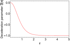
Figure 1: Background deceleration parameter $\bar{q}(\tau)$ in the FLRW geometry in terms of a dimensionless variable $\tau$. The background scenario in the $\Lambda$CDM model are graphically the same comparing it with the one in the $f(R)$ Hu-Sawicki model in the Jordan frame.

Now, we focus on the background field equations in the Jordan frame gravity. Starting from the 01, 00, 11 components of the gravitational field equations in the LTB metric and the scalar field equation, if we do not include local inhomogeneities, we get the respective equation system in the Jordan frame for the background FLRW metric (see the field equations in Ref. 8). We use the Hu-Sawicki model in the Jordan frame, which is characterized by the scalar field potential in Eq. (3).

To solve numerically the equation system, we fix $\Omega_{m0}$ at the same value used in the previous study for the $\Lambda$CDM model, and we choose [10] $\left|F_{R0}\right|=10^{-7}$ to obtain $c_{1}=2.0\cdot 10^{6}$ and $c_{2}=1.5\cdot 10^{5}$. We set the free parameters in a way that the Hu-Sawicki model in the Jordan frame is very close to the $\Lambda$CDM scenario for the background level. In Fig. 2 note that the scalar field potential (3) exhibits a slow-roll mimicking a cosmological constant.

Finally, we solve numerically the equation system in the Jordan frame [4], imposing the conditions at $\tau=1:$ $\bar{\phi}\left(1\right)=1-\left|F_{R0}\right|$ and $d\bar{\phi}/d\tau\left(1\right)=0$. The resulting plot of the deceleration parameter $\bar{q}\left(\tau\right)$ are graphically undistinguishable from the respective ones in the $\Lambda$CDM model (see Fig. 1). Concerning the evolution of the scalar field, we plot in Fig. 2 the deviation $\left|1-\bar{\phi}\left(\tau\right)\right|$ from the GR limit ($\bar{\phi}=1$) with a scale $10^{-7}$. Note that the dynamics of the Jordan frame is very close to the one in $\Lambda$CDM model at the background order for any $\tau$. Now, we can move on to the linearized solutions to highlight the differences between the two cosmological models.

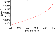
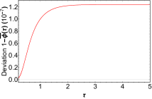
Figure 2: Plots referred to the Hu-Sawicki model in the Jordan frame, adopting the FLRW metric (background solution). Left panel: scalar field potential of the Hu-Sawicki model in the Jordan frame. Right panel: deviation $|1-\bar{\phi}\left(\tau\right)|$ from the GR scenario ($\bar{\phi}=1$) using a scale $10^{-7}$.

3.2 Comparing linear solutions

To examine separately the time and radial evolution of local inhomogeneities, we use the separable variables method at the first-order perturbation theory. So, we factorize all the linear perturbations into time and radial functions. More specifically, we rewrite the perturbations of the scale factor $\delta a\left(\tau,r\right)\equiv\delta\texttt{a}\left(\tau\right)\,\delta\mathfrak{a}\left(r\right)$, the metric functions $\delta\alpha\left(\tau,r\right)\equiv\delta A\left(\tau\right)\,\delta\mathcal{A}\left(r\right)$ and $\delta\beta\left(\tau,r\right)\equiv\delta B\left(\tau\right)\,\delta\mathcal{B}\left(r\right)$, the energy density $\delta\rho\left(\tau,r\right)\equiv\delta P\left(\tau\right)\,\delta\varrho\left(r\right)$, and the scalar field $\delta\phi\left(\tau,r\right)\equiv\delta\Phi\left(\tau\right)\,\delta\varphi\left(r\right)$. The factorization is assumed at the linear level to find analytical solutions, but the separation of variables is not a general method, if we also include non-linear terms.

Then, we investigate the effect of inhomogeneities in the dynamics, according to the cosmological model considered. We focus on the linearized equations in the LTB metric within the framework of the $\Lambda$CDM cosmological model.

Using the factorization abovementioned, it is easy to show that the 11 component of the linearized Einstein equations in the LTB metric can be separated in two parts [4]. The radial behavior is $\delta\mathfrak{a}\left(r\right)=K^{2}\left(r\right)\,,$while we have an ordinary differential equation in terms of $\tau$ for the time evolution:

$$\delta\ddot{\texttt{a}}\left(\tau\right)+\frac{\dot{\bar{a}}\left(\tau\right)}{\bar{a}\left(\tau\right)}\,\delta\dot{\texttt{a}}\left(\tau\right)-\delta\texttt{a}\left(\tau\right)\,\left[\frac{\ddot{\bar{a}}\left(\tau\right)}{\bar{a}\left(\tau\right)}+\left(\frac{\dot{\bar{a}}\left(\tau\right)}{\bar{a}\left(\tau\right)}\right)^{2}\right]=0\,.$$ (9)

This equation is solved numerically, once you specify the background solution (8). We impose the following conditions at $\tau=1$ today: $\delta\texttt{a}\left(1\right)=10^{-5}$ and $\delta\dot{\texttt{a}}\left(1\right)=0$. In Fig. 3 we plot the numerical solution, after we have defined the ratio $\eta\left(\tau\right)$ between the perturbed scale factor and the background respective quantity, namely $\eta\left(\tau\right)\equiv\left|\delta\texttt{a}\left(\tau\right)\,/\,\bar{a}\left(\tau\right)\right|$. Note that perturbations of the scale factor remain stable, since the background scale factor $\bar{a}\left(\tau\right)$ dominates for any $\tau$ in the late Universe, i.e. $\eta\ll 1$.

After that, we consider the 00 component of the linearized Einstein equations in the LTB metric, and we combine it with the continuity equation. After long but straightforward calculations [4], we obtain $\delta\mathfrak{a}\propto 1/r^{3}$ in GR. According to the cosmological principle, inhomogeneities decay for increasing values of $r$. Furthermore, we also obtain that the perturbation of the energy density for a matter component follows the same dependence of the respective background quantity in the FLRW metric, namely $\delta P\left(\tau\right)\propto 1/\bar{a}^{3}\left(\tau\right)$. However, we can provide $\delta P\left(\tau\right)\ll\bar{\rho}\left(\tau\right)$ at any times, setting the constant of integration.

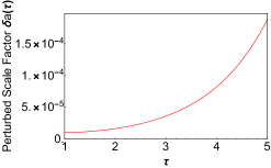
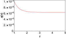
Figure 3: Left panel: time evolution of the linear perturbation of the scale factor $\delta\text{a}\left(\tau\right)$. Right panel: the ratio between the linear deviation and background scale factor.

Now, we repeat the same approach in the modified gravity dynamics in the Jordan frame, considering the corresponding linearized field equations in the LTB metric. Expanding the scalar field potential and its derivative around the background scalar field, as mentioned at the beginning of Sec. 3, it can be proved that the potential $V\left(\phi\right)$ is involved only in the time evolution of the linearized field equations [4]. As a result, we expect that the radial evolution of local inhomogeneities is completely independent of the choice of a particular $f\left(R\right)$ model, since $V\left(\phi\right)$ is directly related to $f\left(R\right)$.

In what follows, we do not focus on the time evolution of perturbations, but we just mention that we find a numerical solution using again the Hu-Sawicki model (Sec. 1), and we have checked that inhomogeneous perturbations remain smaller than respective background contribution for any time $\tau$.

To obtain an analytical solution for the radial part with the separable variables method, we assume two simplifying conditions: $\delta\dot{A}\left(\tau\right)=\delta\dot{B}\left(\tau\right)$ and $\delta\varrho\left(r\right)\propto\delta\varphi\left(r\right)$. After long but straightforward calculations [4], combining the linearized field equations, we obtain a Yukawa-like solution for the radial part of the linear perturbation of the scalar field

$$\delta\varphi\left(r\right)=\frac{C}{r}\,\exp\left(-\frac{r}{r_{c}}\right)\,,$$ (10)

where $C$ and $r_{c}$ are constants. Moreover, $\delta\varrho\left(r\right)$ shows the same evolution, since we recall that it is proportional to $\delta\varphi\left(r\right)$. We also obtain a similar behavior for $\delta\mathcal{A}\left(r\right)$ and $\delta\mathcal{B}\left(r\right)$. It should be emphasized that modified gravity introduces a typical spatial scale, $r_{c}$, such that for $r\gg r_{c}$ the inhomogeneities decay faster than ones in GR. We stress again that this kind of solutions applies to any $f(R)$ model, and the radial evolution is different from the one in GR.

4 Summary and conclusions

We have investigated local inhomogeneities in the LTB metric regarded as small deviations from a flat FLRW background metric. To date, there are no modified gravity models that predict significant deviations from GR, reconciling all possible cosmological data. Hence, to try to discriminate between several cosmological models, it is crucial to test gravity in different regimes or by using other techniques. Here, we have suggested one possible method, studying the different dynamics of inhomogeneous perturbations. Our results have pointed out a distinctive element in the evolution of local inhomogeneities of the Universe from a theoretical point of view, allowing to distinguish between the $\Lambda$CDM cosmological model and $f\left(R\right)$ modified gravity theories. We have shown that the radial evolution of inhomogeneous perturbations within the framework of the Jordan frame gravity is independent of the scalar field potential $V(\phi)$: the distinctive radial solution is a feature of any $f(R)$ model. Furthermore, we have obtained a Yukawa-like solution for the radial perturbations in the Jordan frame, which is completely different from the one in GR. This work may be an interesting arena to account for the effects of local inhomogeneities in cosmological observables [15], when forthcoming missions such as Euclid Deep Survey [16], will be able to test the large-scale properties of the Universe.

References

- [1] S. Weinberg, Cosmology (Oxford University Press, 2008)
- [2] P. J. E. Peebles, Principles of Physical Cosmology (Princeton University Press, 1993)
- [3] N. Aghanim, Y. Akrami, M. Ashdown, et al., Planck 2018 results. VI. Cosmological parameters, AA 641, A6 (2020)
- [4] T. Schiavone, G. Montani, P. Marcoccia, Signature of gravity via Lemaître-Tolman-Bondi inhomogeneous perturbations, to be submitted
- [5] E. Di Valentino, O. Mena, P. Supriya, et al., In the realm of the Hubble tension — a review of solutions, Class. Quantum Grav. 38, 153001 (2021)
- [6] M. G. Dainotti, B. De Simone, T. Schiavone, G. Montani, E. Rinaldi, and G. Lambiase, On the Hubble Constant Tension in the SNe Ia Pantheon Sample, ApJ 912(2), 150 (2021)
- [7] S. Nojiri, and S. D. Odintsov, Introduction to modified gravity and gravitational alternative for dark energy, IJGMM 4, 115 (2007)
- [8] T. P. Sotiriou, and V. Faraoni, theories of gravity, Rev. Mod. Phys. 82, 451 (2010)
- [9] S. Capozziello, and V. Faraoni, Beyond Einstein gravity (Springer, 2013)
- [10] W. Hu, and I. Sawicki, Models of cosmic acceleration that evade solar system tests, Phys. Rev. D 76, 064004 (2007)
- [11] P. Marcoccia, and G. Montani, Weakly Inhomogeneous models for the Low-Redshift Universe, arXiv:1808.01489
- [12] A. A. Starobinsky, Disappearing cosmological constant in gravity, JETP Lett. 86, 157 (2007)
- [13] S. Tsujikawa, Observational signatures of dark energy models that satisfy cosmological and local gravity constraints, Phys. Rev. D 77, 023507 (2008)
- [14] A. de la Cruz-Dombriz, P. K. S. Dunsby, S. Kandhai, and D. Saez-Gomez, Theoretical and observational constraints of viable theories of gravity, Phys. Rev. D 93, 084016 (2016)
- [15] G. Fanizza, B. Fiorini, and G. Marozzi, Cosmic variance of in light of forthcoming high-redshift surveys, Phys. Rev. D 104, 083506 (2021)
- [16] L. Amendola, S. Appleby, A. Avgoustidis., et al., Cosmology and fundamental physics with the Euclid satellite, Living Rev. Relativ. 21, 2 (2018)