Amortized Variational Inference in Simple Hierarchical Models

Abstract

It is difficult to use subsampling with variational inference in hierarchical models since the number of local latent variables scales with the dataset. Thus, inference in hierarchical models remains a challenge at large scale. It is helpful to use a variational family with structure matching the posterior, but optimization is still slow due to the huge number of local distributions. Instead, this paper suggests an amortized approach where shared parameters simultaneously represent all local distributions. This approach is similarly accurate as using a given joint distribution (e.g., a full-rank Gaussian) but is feasible on datasets that are several orders of magnitude larger. It is also dramatically faster than using a structured variational distribution.

1 Introduction

Hierarchical Bayesian models are a general framework where parameters of “groups” are drawn from some shared distribution, and then observed data is drawn from a distribution specified by each group’s parameters. After data is observed, the inference problem is to infer both the parameters for each group and the shared parameters. These models have proven useful in various domains [12] including hierarchical regression amd classification [11], topic models [4, 21, 3], polling [10, 23], epidemiology [22], ecology [7], psychology [35], matrix-factorization [33], and collaborative filtering [25, 31].

A proven technique for scaling variational inference (VI) to large datasets is subsampling. The idea is that if the target model has the form $p(z,y)=p(z)\prod_{i}p(y_{i}|z)$ then an unbiased gradient can be estimated while only evaluating $p(z)$ and $p(y_{i}|z)$ at a few $i$ [15, 19, 29, 28, 34, 14].

This paper addresses hierarchical models of the form $p(\theta,z,y)=p(\theta)\prod_{i}p(z_{i},y_{i}|\theta)$, where only $y$ is observed. There are two challenges. First, the number of local latent variables $z_{i}$ increases with the dataset, meaning the posterior distribution increases in dimensionality. Second, there is often a dependence between $z_{i}$ and $\theta$ which must be captured to get strong results [14].

The aim of this paper is to develop a black-box variational inference scheme that can scale to large hierarchical models without losing benefits of a joint approximation. Our solution takes three steps. First, in the true posterior, the different latent variables $z_{i}$ are conditionally independent given $\theta$, which suggests using a variational family of the same form. We confirm this intuition by showing that for any joint variational family $q(\theta,z)$, one can define a corresponding "branch" family $q(\theta)\prod_{i}q(z_{i}|\theta)$ such that inference will be equally accurate (2). We call inference using such a family the "branch" approach.

Second, we observe that if using the branch approach, the optimal local variational parameters can be computed only from $\theta$ and local data (eq. 12). Thus, we propose to amortize the computation of the local variational parameters by learning a network to approximately solve that optimization. We show that when the target distribution is symmetric over latent variables, this will be as accurate as the original joint family, assuming a sufficiently capable amortization network (5).

Third, we note that in many real hierarchical models, there are many i.i.d. data generated from each local latent variable. This presents a challenge for learning an amortization network, since the full network should deal with different numbers of data points and naturally reflect the symmetry between the inputs (that is, without having to relearn the symmetry.) We propose an approach where a preliminary "feature" network processes each datum, after which they are combined with a pooling operation which forms the input for a standard network (section 6). This is closely related to the "deep sets" [37] strategy for permutation invariance.

We validate these methods on a synthetic model where exact inference is possible, and on a user-preference model for the MovieLens dataset with 162K users who make 25M ratings of different movies. At small scale (2.5K ratings), we show similar accuracy using a dense joint Gaussian, a branch distribution, or our amortized approach. At moderate scale (180K ratings), joint inference is intractable. Branch distributions gives a meaningful answer, and the amortized approach is comparable or better. At large scale (18M ratings) the amortized approach is thousands of nats better on test-likelihoods even after branch distributions were trained for almost ten times as long as the amortized approach took to converge (fig. 6).

2 Hierarchical Branched Distributions

Figure 1: The graphical model for the HBDs. On the left, we have plate notation for the generic HBD from eq. 3. Note, we can have an edge from $\theta$ to $y_{ij}$ (we skip it for clarity.) On the right, we have an example model with $N=3$.

We focus on two-level hierarchical distributions. A generic model of this type is given by

$$p(\theta,z,y|x) =p(\theta)\prod_{i=1}^{N}p(z_{i}|\theta)p(y_{i}|\theta,z_{i},x_{i}),$$ (1)

where $\theta$ and $z=\{z_{i}\}_{i=1}^{N}$ are latent variables, $y=\{y_{i}\}_{i=1}^{N}$ are observations, and $x=\{x_{i}\}_{i=1}^{N}\allowbreak$ are covariates. As the visual representations of these models resemble branches, we refer them as hierarchical branch distributions (HBDs).

Symmetric.

We call an HBD symmetric if the conditionals are symmetric, i.e., if $z_{i}=z_{j},x_{i}=x_{j},$ and $y_{i}=y_{j}$, it implies that

$$p(z_{i}|\theta) =p(z_{j}|\theta)\text{, and }$$

$$p(y_{i}|\theta,z_{i},x_{i}) =p(y_{j}|\theta,z_{j},x_{j}).$$ (2)

Locally i.i.d.

Often local observations $y_{i}$ (and $x_{i}$) are a collection of conditionally i.i.d observations. Then, an HBD takes the form of

$$p(\theta,z,y|x) =p(\theta)\prod_{i=1}^{N}p(z_{i}|\theta)\prod_{j=1}^{n_{i}}p(y_{ij}|\theta,z_{i},x_{ij}),$$ (3)

where $y_{i}=\{y_{ij}\}_{j=1}^{n_{i}}$ and $x_{i}=\{x_{ij}\}_{j=1}^{n_{i}}$ are collections of conditionally i.i.d observations and covariates; $n_{i}\geq 1$ is the number of observations for branch $i$.

No local covariates.

Some applications do not involve the covariates $x_{i}$. In such cases, HBDs have a simplified form of

$$p(\theta,z,y) =p(\theta)\prod_{i=1}^{N}p(z_{i}|\theta)p(y_{i}|\theta,z_{i}).$$ (4)

In this paper, we will be using eq. 1 and eq. 3 to refer HBDs—the results extend easily to case where there are no local covariates. (For instance, in section 5, we amortize using $(x_{i},y_{i})$ as inputs. When there are no covariates, we can amortize with just $y_{i}$.)

2.1 Related Work

Bayesian inference in hierarchical models is an old problem. The most common solutions are Markov chain Monte Carlo (MCMC) and VI. A key advantage of VI is that gradients can sometimes be estimated using only a subsample of data. Hoffman et al. [15] observe that inference in hierarchical models is still slow at large scale, since the number of parameters scales with the dataset. Instead, they assume that $\theta$ and $z_{i}$ from eq. 1 are in conjugate exponential families, and observe that for a mean-field variational distribution $q(\theta)\prod_{i}q(z_{i})$, the optimal $q(z_{i})$ can be calculated in closed form for fixed $q(\theta)$. This is highly scalable, though it is limited to factorized approximations and requires a conditionally conjugate target model.

A structured variational approximation like $q(\theta)\prod_{i}q(z_{i}|\theta)$ can be used which reflects the dependence of $z_{i}$ on $\theta$ [14, 32, 2, 17]. However, this still has scalability problems in general since the number of parameters grows in the size of the data (section 7). To the best of our knowledge, the only approach that avoids this is the framework of structured stochastic VI [14, 17], which assumes the target is conditionally conjugate, and that for a fixed $\theta$ an optimal "local" distribution $q(z_{i}|\theta)$ can be calculated from local data. Hoffman and Blei [14] address matrix factorization models and latent Dirichlet allocation, using Gibbs sampling to compute the local distributions. Johnson et al. [17] use amortization for conjugate models but do not consider the setting where local observations are a collection of i.i.d observations. Our approach is not strictly an instance of either of these frameworks, as we do not assume conjugacy or that amortization can exactly recover optimal local distributions [14, Eq. 7]. Still the spirit is the same, and our approach should be seen as part of this line of research.

Amortized variational approximations have been used to learn models with local variables [19, 9, 16, 5]. A particularly related instance of model learning is the Neural Statistician approach [9], where a “statistics network” learns representations of closely related datasets–the construction of this network is similar to our “pooling network” in section 6. However, in the Neural Statistician model there are no global variables $\theta$, and it is not obvious how to generalize their approach for HBDs. In contrast, our “pooling network” results from the analysis in section 5, reducing the architectural space when $\theta$ is present while retaining accuracy. Moreover, learning a model is strictly different from our “black-box" setting where we want to approximate the posterior of a given model, and the inference only has access to $\log p$ or $\nabla_{\theta,z}\log p$ (or their parts) [28, 20, 2, 1].

3 Joint approximations for HBD

When dealing with HBDs, a non-structured distribution does not scale. To see this, consider the naive VI objective—Evidence Lower Bound (ELBO, $\mathcal{L}$). Let $\smash{q_{\phi}^{\mathrm{Joint}}}$ be a joint variational approximation over $\uptheta$ and $\mathsf{z}$; we use sans-serif font for random variables. Then,

$$\mathcal{L}\left(\smash{q_{\phi}^{\mathrm{Joint}}}\middle\|p\right)=\mathbb{E}_{\smash{q_{\phi}^{\mathrm{Joint}}}(\uptheta,\mathsf{z})}\left[\log\frac{p(\uptheta,\mathsf{z},y|x)}{\smash{q_{\phi}^{\mathrm{Joint}}}(\uptheta,\mathsf{z})}\right],$$ (5)

where $\phi$ are variational parameters. Usually the above expectation is not tractable and one uses a Monte-Carlo estimator. A single sample estimator is given by

$$\widehat{\mathcal{L}}=\log\frac{p(\uptheta,\mathsf{z},y|x)}{\smash{q_{\phi}^{\mathrm{Joint}}}(\uptheta,\mathsf{z})},$$ (6)

where $(\uptheta,\mathsf{z})\sim\smash{q_{\phi}^{\mathrm{Joint}}}$ and $\widehat{\mathcal{L}}$ is unbiased. Since $\smash{q_{\phi}^{\mathrm{Joint}}}$ need not factorize, even a single estimate requires sampling all the latent variables at each step. This is problematic when there are a large number of local latent variables. One encounters the same scaling problem when taking the gradient of the ELBO. We can estimate the gradient using any of the several available estimators [28, 19, 29, 30]; however, none of them scale if $\smash{q_{\phi}^{\mathrm{Joint}}}$ does not factorize [15].

4 Branch approximations for HBD

It is easy to see that the posterior distribution of the HBD eq. 1 takes the form

$$p(\theta,z|y,x)=p(\theta|y,x)\prod_{i=1}^{N}p(z_{i}|\theta,y_{i},x_{i}).$$

As such, it is natural to consider variational distributions that factorize the same way (see fig. 2.) In this section, we confirm this intuition—we start with any joint variational family which can have any dependence between $\theta$ and $z_{1},\cdots,z_{N}$. Then, we define a corresponding “branch” family where $z_{1},\cdots,z_{N}$ are conditionally independent given $\theta$. We show that inference using the branch family will be at least as accurate as using the joint family. We formalize the idea of branch distribution in the next definition.

Definition 1.

Let $\smash{q_{\phi}^{\mathrm{Joint}}}$ be any variational family with parameters $\phi$. We define $\smash{q_{v,w}^{\mathrm{Branch}}}$ to be a corresponding branch family if, for all $\phi$, there exists $(v,\{w_{i}\}_{i=1}^{N})$, such that,

$$\smash{q_{v,w}^{\mathrm{Branch}}}(\theta,z)=q_{v}(\theta)\prod_{i=1}^{N}q_{w_{i}}(z_{i}|\theta)=\smash{q_{\phi}^{\mathrm{Joint}}}(\theta)\prod_{i=1}^{N}\smash{q_{\phi}^{\mathrm{Joint}}}(z_{i}|\theta).$$ (7)

Figure 2: $\ qb$ as in eq. 7.

Given a joint distribution, a branch distribution can always be defined by choosing $w$ and $v_{i}$ as the components of $\phi$ that influence $\smash{q_{\phi}^{\mathrm{Joint}}}(\theta)$ and $\smash{q_{\phi}^{\mathrm{Joint}}}(z_{i}|\theta)$, respectively, and choosing $q_{w}(\theta)$ and $q_{w_{i}}(z_{i}|\theta)$ correspondingly. However, the choice is not unique (for instance, the parameterization can require transformations—different transformations can create different variants.)

The idea to use $\smash{q_{v,w}^{\mathrm{Branch}}}$ is natural [14, 2]. However, one might question if the branch variational family is as good as the original $\smash{q_{\phi}^{\mathrm{Joint}}}$; in 2, we establish that this is indeed true.

Theorem 2.

Let $p$ be a HBD, and $\smash{q_{\phi}^{\mathrm{Joint}}}(\theta,z)$ be a joint approximation family parameterized by $\phi$. Choose a corresponding branch variational family $\smash{q_{v,w}^{\mathrm{Branch}}}(\theta,z)$ as in definition 1. Then,

$$\min_{v,w}KL\left(\smash{q_{v,w}^{\mathrm{Branch}}}\middle\|p\right)\leq\min_{\phi}KL\left(\smash{q_{\phi}^{\mathrm{Joint}}}\middle\|p\right).$$

We stress that $\smash{q_{v,w}^{\mathrm{Branch}}}$ is a new variational family derived from but not identical to $\smash{q_{\phi}^{\mathrm{Joint}}}$. 2 implies that we can optimize a branched variational family $\smash{q_{v,w}^{\mathrm{Branch}}}$ without compromising the quality of approximation (see appendix C for proof.) In the following corollary, we apply 2 to a joint Gaussian to show that using a branch Gaussian will be equally accurate.

Corrolary 3.

Let $p$ be a HBD, and let $\smash{q_{\phi}^{\mathrm{Joint}}}(\theta,z)=\mathcal{N}\left((\theta,z)|\mu,\Sigma\right)$ be a joint Gaussian approximation (with $\phi=(\mu,\Sigma)$). Choose a variational family

$$\smash{q_{v,w}^{\mathrm{Branch}}}(\theta,z)=\mathcal{N}(\theta|\mu_{0},\Sigma_{0})\prod_{i=1}^{N}\mathcal{N}(z_{i}|\mu_{i}+A_{i}\theta,\ \Sigma_{i})$$

with $v=(\mu_{0},\Sigma_{0})$ and $w_{i}=(\mu_{i},\Sigma_{i},A_{i}).$ Then, $\displaystyle\min_{v,w}KL\left(\smash{q_{v,w}^{\mathrm{Branch}}}\middle\|p\right)\leq\min_{\phi}KL\left(\smash{q_{\phi}^{\mathrm{Joint}}}\middle\|p\right).$

In the above corollary, the structured family $\smash{q_{v,w}^{\mathrm{Branch}}}$ is chosen such that it can represent any branched Gaussian distribution. Notice, the mean of the conditional distribution is an affine function of $\theta$. This affine relationship appears naturally when you factorize the joint Gaussian over $\left(\uptheta,\mathsf{z}\right)$. For more details see appendix E.

JointELBO$(\phi,y,x)$

     $\theta,z\sim\smash{q_{\phi}^{\mathrm{Joint}}}(\uptheta,\mathsf{z})$

     ${\displaystyle\widehat{\mathcal{L}}\leftarrow\log\frac{p(\theta,z,y|x)}{\smash{q_{\phi}^{\mathrm{Joint}}}(\theta,z)}}$

(a) Estimation with $\smash{q_{\phi}^{\mathrm{Joint}}}$ as in eq. 6

BranchELBO$(v,w,y,x)$

     $\theta\sim q_{v}(\uptheta)$

     $z_{i}\sim q_{w_{i}}(\mathsf{z}_{i}|\theta)$ for $i\in\{1,\cdots,N\}$.

     ${\displaystyle\widehat{\mathcal{L}}\leftarrow\log\frac{p\left(\theta\right)}{q_{v}\left(\theta\right)}+\sum_{i=1}^{N}\log\frac{p\left(z_{i},y_{i}|\theta,x_{i}\right)}{q_{w_{i}}\left(z_{i}|\theta\right)}}$

(b) Estimation with $\smash{q_{v,w}^{\mathrm{Branch}}}$ as in eq. 9

SubSampledBranchELBO$(v,w,y,x)$

     $\theta\sim q_{v}(\uptheta)$

     $B\sim\texttt{Minibatch($\mathsf{B}$)}$

     $z_{i}\sim q_{w_{i}}(\mathsf{z}_{i}|\theta)$ for $i\in B$

     ${\displaystyle\widehat{\mathcal{L}}\leftarrow\log\frac{p\left(\theta\right)}{q_{v}\left(\theta\right)}+\frac{N}{\left|B\right|}\sum_{i\in B}\log\frac{p\left(z_{i},y_{i}|\theta,x_{i}\right)}{q_{w_{i}}\left(z_{i}|\theta\right)}}$

(c) Estimation with $\smash{q_{v,w}^{\mathrm{Branch}}}$ as in eq. 10

AmortizedSubSampledBranchELBO$(v,u,y,x)$

     $\theta\sim q_{v}(\uptheta)$

     $B\sim\texttt{Minibatch($\mathsf{B}$)}$

     $w_{i}\leftarrow{\texttt{net}}_{u}(x_{i},y_{i})$ for $i\in B$

     $z_{i}\sim q_{w_{i}}(\mathsf{z}_{i}|\theta)$ for $i\in B$

     ${\displaystyle\widehat{\mathcal{L}}\leftarrow\log\frac{p\left(\theta\right)}{q_{v}\left(\theta\right)}+\frac{N}{\left|B\right|}\sum_{i\in B}\log\frac{p\left(z_{i},y_{i}|\theta,x_{i}\right)}{q_{w_{i}}\left(z_{i}|\theta\right)}}$

(d) Estimation with $\smash{q_{v,u}^{\mathrm{Amort}}}$ for $p$ as in eq. 2

Figure 3: Pseudo codes for ELBO estimation with different variational methods; $w=\{w_{i}\}_{i=1}^{N}$, $y=\{y_{i}\}_{i=1}^{N}$, and $y_{i}=\{y_{ij}\}_{j=1}^{n_{i}}$ ($x$ is defined similar to $y$.) (a) Estimates ELBO for a joint approximation; (b) to (d) estimate ELBO for branch approximations; (c, d) use subsampling to estimate ELBO; (d) uses amortized conditionals; (a) to (c) work for any HBD, and (d) assumes $p$ is a symmetric HBD as in eq. 2. For models where $n_{i}>1$, we use the ${\texttt{net}}_{u}$ as in fig. 4. Minibatch is some distribution over the set of possible minibatches and $\left|B\right|$ denotes the number of samples in a minibatch $B$.

4.1 Subsampling in branch distributions

In this section, we show that if $p$ is an HBD and $\smash{q_{v,w}^{\mathrm{Branch}}}$ is as in definition 1, we can estimate ELBO using local observations and scale better. Consider the ELBO

$$\mathcal{L}\left(\smash{q_{v,w}^{\mathrm{Branch}}}\middle\|p\right) =\operatornamewithlimits{\mathbb{E}}_{\smash{q_{v,w}^{\mathrm{Branch}}}\left(\uptheta,\mathsf{z}\right)}\left[\log\frac{p\left(\uptheta,\mathsf{z},y|x\right)}{\smash{q_{v,w}^{\mathrm{Branch}}}\left(\uptheta,\mathsf{z}\right)}\right]$$

$$=\operatornamewithlimits{\mathbb{E}}_{q_{v}\left(\uptheta\right)}\left[\log\frac{p\left(\uptheta\right)}{q_{v}\left(\uptheta\right)}\right]+\sum_{i=1}^{N}\operatornamewithlimits{\mathbb{E}}_{q_{v}\left(\uptheta\right)}\operatornamewithlimits{\mathbb{E}}_{q_{w_{i}}\left(\mathsf{z}_{i}|\theta\right)}\left[\log\frac{p\left(\mathsf{z}_{i},y_{i}|\theta,x_{i}\right)}{q_{w_{i}}\left(\mathsf{z}_{i}|\theta\right)}\right].$$ (8)

Without assuming special structure (e.g. conjugacy) the above expectations will not be available in closed form. To estimate the ELBO, let $(\uptheta,\left\{\mathsf{z}_{i}\right\}_{i=1}^{N})\sim\smash{q_{v,w}^{\mathrm{Branch}}}$. Then, an unbiased estimator is

$$\widehat{\mathcal{L}} =\log\frac{p\left(\uptheta\right)}{q_{v}\left(\uptheta\right)}+\sum_{i=1}^{N}\left[\log\frac{p\left(\mathsf{z}_{i},y_{i}|\uptheta,x_{i}\right)}{q_{w_{i}}\left(\mathsf{z}_{i}|\uptheta\right)}\right].$$ (9)

Unlike the joint estimator of eq. 6, one can subsample the terms in eq. 9 to create a new unbiased estimator. Let $\mathsf{B}$ be randomly selected minibatch of indices from $\{1,2,\dots,N\}$. Then,

$$\widehat{\mathcal{L}} =\log\frac{p\left(\uptheta\right)}{q_{v}\left(\uptheta\right)}+\frac{N}{\left|\mathsf{B}\right|}\sum_{i\in\mathsf{B}}\left[\log\frac{p\left(\mathsf{z}_{i},y_{i}|\uptheta,x_{i}\right)}{q_{w_{i}}\left(\mathsf{z}_{i}|\uptheta\right)}\right],$$ (10)

is another unbiased estimator of ELBO. In LABEL:sub@fig:_pseudocode_branch, LABEL: and LABEL:sub@fig:_pseudocode_branch_subsampled, we present the complete pseudocodes for ELBO estimation with and without subsampling in branch distributions.

Unsurprisingly, the same summation structure appears for gradients estimators of branch ELBO, allowing for efficient gradient estimation. With subsampled evaluation and training, branch distributions are immensely computationally efficient—in our experiments, we scale to models with $10^{3}$ times more latent variables by switching to branch approximations (see fig. 6).

While branch distributions are immensely more scalable than joint approximations, the number of parameters still scales as $\mathcal{O}(N)$. In the next section, we demonstrate that for symmetric HBDs, we can share parameters for the local conditionals (amortize) to allow further scalability.

5 Amortized branch approximations

In this section, we discuss how one can amortize the local conditionals of a branch approximations when the target HBD is symmetric (see eq. 2.) We first formally introduce the amortized branch distributions in the next definition and then justify the amortization for symmetric HBD.

Definition 4.

Let $\smash{q_{\phi}^{\mathrm{Joint}}}$ be a joint approximation and let $\smash{q_{v,w}^{\mathrm{Branch}}}$ be as in definition 1. Suppose ${\texttt{net}}_{u}(x_{i},y_{i})$ is some parameterized map (with parameters $u$) from local observations $(x_{i},y_{i})$ to space of $w_{i}$. Then,

$$\smash{q_{v,u}^{\mathrm{Amort}}}(\theta,z)=q_{v}(\theta)\prod_{i=1}^{N}q_{{{\texttt{net}}}_{u}(x_{i},y_{i})}(z_{i}|\theta)$$ (11)

is a corresponding amortized branch distribution.

The idea to amortize is natural once you examine the optimization for symmetric HBDs. Consider the optimization for objective in eq. 8.

$$\max_{v,w}\mathcal{L}\left(\smash{q_{v,w}^{\mathrm{Branch}}}\middle\|p\right) =\max_{v,w}\left[\operatornamewithlimits{\mathbb{E}}_{q_{v}\left(\uptheta\right)}\left[\log\frac{p\left(\uptheta\right)}{q_{v}\left(\uptheta\right)}\right]+\sum_{i=1}^{N}\operatornamewithlimits{\mathbb{E}}_{q_{v}\left(\uptheta\right)}\operatornamewithlimits{\mathbb{E}}_{q_{w_{i}}\left(\mathsf{z}_{i}|\uptheta\right)}\left[\log\frac{p\left(\mathsf{z}_{i},y_{i}|\uptheta,x_{i}\right)}{q_{w_{i}}\left(\mathsf{z}_{i}|\uptheta\right)}\right]\right]$$

$$=\max_{v}\left[\operatornamewithlimits{\mathbb{E}}_{q_{v}\left(\uptheta\right)}\left[\log\frac{p\left(\uptheta\right)}{q_{v}\left(\uptheta\right)}\right]+\sum_{i=1}^{N}\max_{w_{i}}\operatornamewithlimits{\mathbb{E}}_{q_{v}\left(\uptheta\right)}\operatornamewithlimits{\mathbb{E}}_{q_{w_{i}}\left(\mathsf{z}_{i}|\uptheta\right)}\left[\log\frac{p\left(\mathsf{z}_{i},y_{i}|\uptheta,x_{i}\right)}{q_{w_{i}}\left(\mathsf{z}_{i}|\uptheta\right)}\right]\right].$$

The crucial observation in the above equation is that for any given $v$, the optimal solution of inner optimization depends only on local data points $\left(x_{i},y_{i}\right)$, i.e.,

$$w^{*}_{i} =\operatornamewithlimits{argmax}_{w_{i}}\operatornamewithlimits{\mathbb{E}}_{q_{v}\left(\uptheta\right)}\operatornamewithlimits{\mathbb{E}}_{q_{w_{i}}\left(\mathsf{z}_{i}|\uptheta\right)}\left[\log\frac{p\left(\mathsf{z}_{i},y_{i}|\uptheta,x_{i}\right)}{q_{w_{i}}\left(\mathsf{z}_{i}|\uptheta\right)}\right].$$ (12)

Now, notice that if $p$ and $\smash{q_{v,w}^{\mathrm{Branch}}}$ have symmetric conditionals, then, for each $i$, we solve the same optimization over $w_{i}$, just with different parameters $y_{i}$ and $x_{i}$. Thus, one could replace the optimization over $w_{i}$ with an optimization over a parameterized function from $(x_{i},y_{i})$ to the space of $w_{i}$. Formally, when the network ${\texttt{net}}_{u}$ is sufficiently capable, we make the following claim.

Claim 5.

Let $p$ be a symmetric HBD and let $\smash{q_{\phi}^{\mathrm{Joint}}}$ be some joint approximation. Let $\smash{q_{v,u}^{\mathrm{Amort}}}$ be as in definition 1. Suppose that for all $v$, there exists a $u$, such that,

$${{\texttt{net}}}_{u}(x_{i},y_{i})=\operatornamewithlimits{argmax}_{w_{i}}\operatornamewithlimits{\mathbb{E}}_{q_{v}\left(\uptheta\right)}\operatornamewithlimits{\mathbb{E}}_{q_{w_{i}}\left(\mathsf{z}_{i}|\uptheta\right)}\left[\log\frac{p\left(\mathsf{z}_{i},y_{i}|\uptheta,x_{i}\right)}{q_{w_{i}}\left(\mathsf{z}_{i}|\uptheta\right)}\right].$$ (13)

Then,

$$\min_{v,u}KL\left(\smash{q_{v,u}^{\mathrm{Amort}}}\middle\|p\right)\leq\min_{\phi}KL\left(\smash{q_{\phi}^{\mathrm{Joint}}}\middle\|p\right)$$ (14)

Note, we only amortize the conditional distribution $q_{w_{i}}\left(z_{i}|\theta\right)$ and leave $q_{v}\left(\theta\right)$ unchanged. In practice, of course, we do not have perfect amortization functions. The quality of the amortization depends on our ability to parameterize and optimize a powerful neural network. In other words, we make the following approximation

$${{\texttt{net}}}_{u}(x_{i},y_{i})\approx\operatornamewithlimits{argmax}_{w_{i}}\operatornamewithlimits{\mathbb{E}}_{q_{v}\left(\uptheta\right)}\operatornamewithlimits{\mathbb{E}}_{q_{w_{i}}\left(\mathsf{z}_{i}|\uptheta\right)}\left[\log\frac{p\left(\mathsf{z}_{i},y_{i}|\uptheta,x_{i}\right)}{q_{w_{i}}\left(\mathsf{z}_{i}|\uptheta\right)}\right].$$ (15)

In our experiments, we found the amortized approaches work well even with moderately sized networks. Due to parameter sharing, the amortized approaches converge much faster than other alternatives (especially, true for larger models; see fig. 6 and table 2).

6 Amortized branch approximations for i.i.d. observations

In the previous section, we discussed how we could amortize branch approximations for symmetric HBDs. However, in some applications, the construction of amortization network ${\texttt{net}}_{u}$ is not as straightforward. Consider the case when we have a varying number of local i.i.d observations for each local latent variable. In this section, we highlight the problem with naive amortization for locally i.i.d HBDs, and present a simple solution to alleviate them.

Mathematically, for locally i.i.d HBDs we have $y_{i}=\{y_{ij}\}_{j=1}^{n_{i}}$ and $x_{i}=\{x_{ij}\}_{j=1}^{n_{i}}$, such that the conditional over $y_{i}$ factorizes as

$$p\left(y_{i}|x_{i},z_{i},\theta\right)=\prod_{j=1}^{n_{i}}p\left(y_{ij}|x_{ij},z_{i},\theta\right).$$

Now, if $x_{i}$ and $y_{i}$ are directly input to the amortization network ${\texttt{net}}_{u}$, the input size to the network would change for different $i$ (notice we have $n_{i}$ observations for $i^{\text{th}}$ local variable.) Another problem is that the optimal variational parameters are invariant to the order in which the i.i.d. observations are presented. For instance, consider two data points: $(x_{i},y_{i})=[(x_{i1},y_{i1}),\dots,(x_{in_{i}},y_{in_{i}})]$ and $(x^{\prime}_{i},y^{\prime}_{i})=[(x_{in_{i}},y_{in_{i}}),\dots,(x_{i1},y_{i1})]$. A naive amortization scheme will evaluate very different conditionals for these two data points because ${\texttt{net}}_{u}(x_{i},y_{i})$ and ${\texttt{net}}_{u}(x^{\prime}_{i},y^{\prime}_{i})$ will be different.

${\texttt{net}}_{u}(x_{i},y_{i})$

     for $j$ in $\{1,2,\dots,n_{i}\}$

          

$e_{j}\leftarrow\texttt{feat\_net}_{u}(x_{ij},y_{ij})$

     $e\leftarrow\texttt{pool}(\{e_{j}\}_{j=1}^{n_{i}})$

     $w_{i}\leftarrow\texttt{param\_net}_{u}(e)$

     return $w_{i}$

Figure 4: Psuedocode for ${\texttt{net}}_{u}$ for locally i.i.d symmetric HBD.

To deal with both issues: variable length input and permutation invariance, we suggest learning a “feature network” and "pooling function" based amortization network; this is reminiscent of "deep sets" [37] albeit here intended not just to enforce permutation invariance but also to deal with inputs of different sizes. Firstly, a feature network feat_net takes each $(x_{ij},y_{ij})$ pair and returns a vector of features $e_{j}$. Secondly, a pooling function pool takes the collection $\{e_{j}\}_{j=1}^{n_{i}}$ and achieves the two aims. First, it collapses $n_{i}$ feature vectors into a single fixed-sized feature $e$ (with the same dimensions as $e_{j}$). Second, pooling is invariant by construction to the order of observations (for example, pooling function would take a dimension-wise mean or sum across $j$.) Finally, this pooled feature vector $e$ is input to another network param_net that returns the final parameters $w_{i}$. The pseudocode for a ${\texttt{net}}_{u}$ with feature networks is available in fig. 4. In table 3, in appendix, we summarize the applicability of proposed variational methods to different HBD variants.

Table 1: All variational families used in our experiments. $\Sigma$ denotes a generic covariance matrix and $\sigma^{2}$ denotes a diagonal covariance.

Gaussian Family	$\smash{q_{\phi}^{\mathrm{Joint}}}$ as in eq. 5	$\smash{q_{v,w}^{\mathrm{Branch}}}$ as in eq. 7	$\smash{q_{v,u}^{\mathrm{Amort}}}$ as in definition 4
Dense	$\mathcal{N}(\theta,z|\mu,\Sigma)$	${\displaystyle\mathcal{N}(\theta|\mu_{0},\Sigma_{0})\prod_{i=1}^{N}\mathcal{N}(z_{i}|\mu_{i}+A_{i}\theta,\Sigma_{i})}$	${\displaystyle\mathcal{N}(\theta|\mu_{0},\Sigma_{0})\prod_{i=1}^{N}\mathcal{N}(z_{i}|\mu_{i}+A_{i}\theta,\Sigma_{i})}$
	$\phi=(\mu,\Sigma)$	$v=(\mu_{0},\Sigma_{0})$, $w_{i}=(\mu_{i},A_{i},\Sigma_{i})$	$v=(\mu_{0},\Sigma_{0}),(\mu_{i},A_{i},\Sigma_{i})={\texttt{net}}_{u}(x_{i},y_{i})$
Block Diagonal	$\mathcal{N}(\theta|\mu_{0},\Sigma_{0})\mathcal{N}(z|\mu_{1},\Sigma_{1})$	${\displaystyle\mathcal{N}(\theta|\mu_{0},\Sigma_{0})\prod_{i=1}^{N}\mathcal{N}(z_{i}|\mu_{i},\Sigma_{i})}$	${\displaystyle\mathcal{N}(\theta|\mu_{0},\Sigma_{0})\prod_{i=1}^{N}\mathcal{N}(z_{i}|\mu_{i},\Sigma_{i})}$
	$\phi=(\mu_{0},\mu_{1},\Sigma_{0},\Sigma_{1})$	$v=(\mu_{0},\Sigma_{0})$, $w_{i}=(\mu_{i},\Sigma_{i})$	$v=(\mu_{0},\Sigma_{0})\text{, }(\mu_{i},\Sigma_{i})={\texttt{net}}_{u}(x_{i},y_{i})$
Diagonal	$\mathcal{N}(\theta,z|\mu,\sigma^{2})$	${\displaystyle\mathcal{N}(\theta|\mu_{0},\sigma_{0}^{2})\prod_{i=1}^{N}\mathcal{N}(z_{i}|\mu_{i},\sigma_{i}^{2})}$	${\displaystyle\mathcal{N}(\theta|\mu_{0},\sigma^{2}_{0})\prod_{i=1}^{N}\mathcal{N}(z_{i}|\mu_{i},\sigma^{2}_{i})}$
	$\phi=(\mu,\sigma^{2})$	$v=(\mu_{0},\sigma^{2}_{0})$, $w_{i}=(\mu_{i},\sigma_{i}^{2})$	$v=(\mu_{0},\sigma_{0}^{2})$, $(\mu_{i},\sigma_{i}^{2})={\texttt{net}}_{u}(x_{i},y_{i})$

7 Experiments

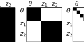
Figure 5: Visualization of covariances of dense, block-diagonal, and diagonal Gaussians. For each, we experiment with $\smash{q_{\phi}^{\mathrm{Joint}}}$, $\smash{q_{v,w}^{\mathrm{Branch}}}$, and $\smash{q_{v,u}^{\mathrm{Amort}}}$ methods.

We conduct experiments on a synthetic and a real-world problem. For each, we consider three inference methods: using a joint distribution, using a branch variational approximation, and using our amortized approach.

For each method, we consider three variational approximations a completely diagonal Gaussian, a block-diagonal Gaussian (with blocks for $\theta$ and $z$) and a dense Gaussian; see fig. 5 for a visual. (For each choice of a joint distribution, the corresponding $\smash{q_{v,w}^{\mathrm{Branch}}}$ is used for the branch variational approximation and the corresponding $\smash{q_{v,u}^{\mathrm{Amort}}}$ for the amortized approach; see table 1 for details.)

We use reparameterized gradients [19] and optimize with Adam [18] (see appendix F for complete experimental details.) In appendix A, we discuss some of the observations we had during experimentation involving parameterization, feat-net architecture, batch-size selection, initialization, and gradient estimators.

7.1 Synthetic problem

The aim of the synthetic experiment is to work with models where we have access to closed-form posterior (and the marginal likelihood.) If the variational family contains the posterior, one can expect the methods to perform close to ideal (provided we can optimize well.)

For our experiments, we use the following hierarchical regression model

$$p(\theta,z,y|x) =\mathcal{N}(\theta|0,I)\prod_{i=1}^{N}\mathcal{N}(z_{i}|\theta,I)\prod_{j=1}^{n_{i}}\mathcal{N}(y_{ij}|x_{ij}^{\top}z_{i},1),$$ (16)

where $\mathcal{N}$ denotes a Gaussian distribution, and $I$ is an identity matrix (see section F.2 for posterior and the marginal closed-form expressions.)

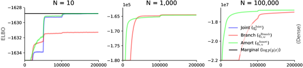
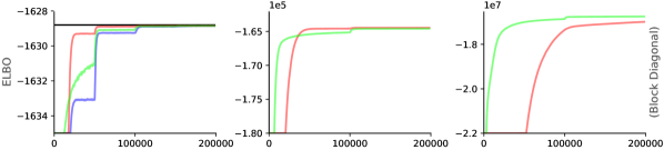
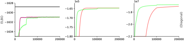
Figure 7: Training ELBO trace for the synthetic problem. Top to bottom: dense, block diagonal, and diagonal Gaussian (for each, we have $\smash{q_{\phi}^{\mathrm{Joint}}}$, $\smash{q_{v,w}^{\mathrm{Branch}}}$, and $\smash{q_{v,u}^{\mathrm{Amort}}}$ method.) Left to right: small, moderate, and large scale of the synthetic problem. For clarity, we plot the exponential moving average of the training ELBO trace with a smoothing value of 0.001. For the small setting, we also plot the true log-marginal $\log p(y|x)$ for reference (black horizontal line): ELBO for dense approach is exactly same as the log-marginal, it’s slightly lower for block, and is much less for the diagonal (see first column.) Note, calculating the log-marginal was computationally prohibitive for the moderate and large setting.

To demonstrate the performance of our methods, we experiment with three different problems scale (correspond to three different models with $N=$ 10, 1K, and $100$K.) Synthetic data is created using forward sampling for each of the scale variants independently. We avoid any test data and metrics for the synthetic problem as the log-marginal is known in closed form. The inference results are present in fig. 7 (in appendix.) In all cases, amortized distributions perform favorably when compared to branch and joint distributions.

Table 2: Inference results for the MovieLens25M problem. For both metrics, we draw a fresh batch of 10,000 samples from the final posterior. All values are in nats (higher is better).

Metric		Final ELBO			Test likelihood
$\approx$ # train ratings		2.5K	180K	18M	2.5K	180K	18M
Methods (see table 1)
Dense	$\smash{q_{\phi}^{\mathrm{Joint}}}$	-1572.31			-166.37
	$\smash{q_{v,w}^{\mathrm{Branch}}}$	-1572.39	-1.0368e+05	-1.1413e+07	-166.66	-11054.43	-1.3046e+06
	$\smash{q_{v,u}^{\mathrm{Amort}}}$	-1572.45	-1.0352e+05	-1.0665e+07	-166.64	-10976.38	-1.1476e+06
Block	$\smash{q_{\phi}^{\mathrm{Joint}}}$	-1579.04			-167.36
Diagonal	$\smash{q_{v,w}^{\mathrm{Branch}}}$	-1579.05	-1.0350e+05	-1.1078e+07	-166.97	-10987.17	-1.2538e+06
	$\smash{q_{v,u}^{\mathrm{Amort}}}$	-1579.06	-1.0353e+05	-1.0665e+07	-166.96	-10975.96	-1.1484e+06
Diagonal	$\smash{q_{\phi}^{\mathrm{Joint}}}$	-1592.59			-167.39
	$\smash{q_{v,w}^{\mathrm{Branch}}}$	-1592.64	-1.0428e+05	-1.1325e+07	-167.31	-10977.95	-1.2713e+06
	$\smash{q_{v,u}^{\mathrm{Amort}}}$	-1592.64	-1.0430e+05	-1.0736e+07	-167.29	-10980.75	-1.1497e+06

7.2 MovieLens

Next, we test our method on the MovieLens25M [13], a dataset of 25 million movie ratings for over 62,000 movies, rated by 162,000 users, along with a set of features (tag relevance scores [36]) for each movie.

Purely, to make experiments more efficient on GPU hardware, we pre-process the data to drop users with more than 1,000 ratings—leaving around $20$M ratings. Also, for the sake of efficiency, we PCA the movie features to reduce their dimensionality to 10. We used a train-test split such that, for each user, one-tenth of the ratings are in the test set. This gives us $\approx$ 18M ratings for training (and $\approx$ 2M ratings for testing.)

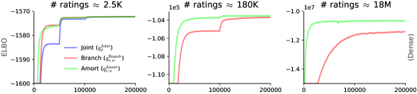
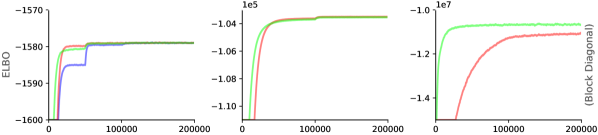
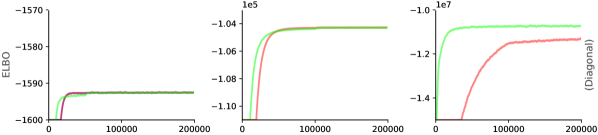
Figure 6: Training ELBO trace for the MovieLens25M problem. Top to bottom: dense, block diagonal, and diagonal Gaussian (for each, we have $\smash{q_{\phi}^{\mathrm{Joint}}}$, $\smash{q_{v,w}^{\mathrm{Branch}}}$, and $\smash{q_{v,u}^{\mathrm{Amort}}}$ method.) Left to right: small, moderate, and large scale of the MovieLens25M problem. For clarity, we plot the exponential moving average of the training ELBO trace with a smoothing value of 0.001. These traces correspond to the values reported in table 2.

We use the hierarchical model

$$p(\theta,z,y|x) =\mathcal{N}(\theta|0,I)\prod_{i=1}^{N}\mathcal{N}(z_{i}|\mu(\theta),\Sigma(\theta))\prod_{j=1}^{n_{i}}\mathcal{B}(y_{ij}|\mathrm{sigmoid}(x_{ij}^{\top}z_{i})),$$ (17)

where $\theta$ represents distribution over user preferences; for instance, $\theta$ might represent that users who like action films tend to also like thrillers but tend to dislike musicals; $z_{i}$ determine the user specific preference; $x_{ij}$ are the features of the $j^{\mathrm{th}}$ movie rated by user $i$; $y_{ij}$ is the binary movie ratings; $n_{i}$ is the number of movies rated by user $i$, and $\mathcal{B}$ denotes a Bernoulli distribution. Here, $\mu$ and $\Sigma$ are functions of $\theta$, such that, for $\theta=[\theta_{\mu},\theta_{\Sigma}]$, we have

$$\mu(\theta)=\theta_{\mu},\quad\quad\text{ and }\quad\quad\Sigma(\theta)=\mathrm{tril}(\theta_{\Sigma})^{\top}\mathrm{tril}(\theta_{\Sigma})$$

where $\mathrm{tril}$ is a function that transforms an unconstrained vector into a lower-triangular positive Cholesky factor. As movie features $x_{ij}\in\mathbb{R}^{10}$, we have $\theta_{\mu}\in\mathbb{R}^{10},\theta_{\Sigma}\in\mathbb{R}^{55}$, and $z_{i}\in\mathbb{R}^{10}$. Note that as $\Sigma$ depends on $\theta$, and the likelihood is Bernoulli, the model is non-conjugate.

For inference, we use the methods as described in table 1. Note, we hold the amortization network architecture constant across the scales–the number of parameters remains fixed for $\smash{q_{v,u}^{\mathrm{Amort}}}$ (for all Gaussian variants) while the number of parameters scale as $\mathcal{O}(N)$ for $\smash{q_{v,w}^{\mathrm{Branch}}}$ (see appendix E for more details.)

In fig. 6, we plot the training time ELBO trace, and in table 2, we present the final training ELBO and test likelihood values. We approximate the test likelihood $p(y^{\mathrm{test}}|x^{\mathrm{test}},x,y)$ with $\mathbb{E}_{q}\left[p(y^{\mathrm{test}}|x^{\mathrm{test}},q)\right]$, and draw a fresh batch of 10,000 samples to approximate the expectation (see appendix F for complete details.) For the smaller model, the amortized and branch approaches perform similar to the joint approach for all three variational approximations; this supports 2 and 5. For the moderate size model, the branch and amortize approaches are very comparable to each other, while joint approaches fail to scale. For the large model (18M ratings), amortized approaches are significantly better than branch methods. We conjecture this is because parameter sharing in amortized approaches improves convergence for models where batch size is smaller compared to total iterates–true only for large model. Interestingly, the performance of amortized Dense and Block Gaussian approximation is very similar in the large and moderate setting (see $\smash{q_{v,u}^{\mathrm{Amort}}}$ results in tables 2, 6 and 7.) We conjecture this is because the posterior over the global parameters is very concentrated for this problem. As $\theta$ behaves like a single fixed value, Block Gaussian performs just as good as the Dense approach (see appendix B for more discussion.)

8 Discussion

In this paper, we present structured amortized variational inference scheme that can scale to large hierarchical models without losing benefits of joint approximations. Such models are ubiquitous in social sciences, ecology, epidemiology, and other fields. Our ideas can not only inspire further research in inference but also provide a formidable baseline for applications.

Appendix A Other practical challenges

Parameterizing covariances

It is common to to re-parameterize covariance matrices to a vector of unconstrained parameters. As above, the typical way to do this is via a function $\mathrm{tril}$ that maps unconstrained vectors to Cholesky factors, i.e. lower-triangular matrices with positive diagonals. This can be done by simple re-arranging the components of the vector into a lower-triangular matrix, followed by applying a function to map the entries on the diagonal components to the positive numbers. In our preliminary experiments, the choice of the mapping was quite significant in terms of how difficult optimization was. Common choices like the ${\exp(x)}$ and ${\log(\exp(x)+1)}$ functions did not perform well when the outputs were close to zero. Instead, we propose to use the transformation $x\mapsto\frac{1}{2}(x+\sqrt{x^{2}+4\gamma})$, where $\gamma$ is a hyperparameter (we use $\gamma=1$). This is based on the proximal operator for the multivariate Gaussian entropy [8, section 5]. Intuitively, when $x$ is a large positive number, this mapping returns approximately $x$, while if $x$ is a large negative number, the mapping returns approximately $-1/x$. This decays to zero more slowly than common mappings, which appears to improve numerical stability and the conditioning of the optimization.

Feature network architecture.

In this paper, we propose the use of a separate feat_net to deal with variable-length input and order invariance. In our preliminary experiments, we found that the performance improves when we concatenate the embedding $e_{j}$ in the fig. 4 with it’s dimension-wise square before sending it to the pooling function pool. We hypothesis that this is because the embeddings act as learnable statistics, and using the elementwise square directly provides useful information to param_net.

Batch size selection

For the small scale problems (both synthetic and MovieLens), we do not subsample data; this is to maintain a fair comparison to joint approaches that do not support subsampling. For moderate and large scales, we select the batch size for the branch methods based on the following rule of thumb: we increase the batch size such that ${\frac{\left|B\right|}{T^{1.18}}}$ is roughly maximized. This rule-of-thumb captures the following intuition. Suppose batch size $\left|B\right|$ takes time $T$ per iteration. If the time taken per iteration for batchsize $\left|2B\right|$ is less than $1.8T$, then we should use $2B$. Of course, we roughly maximize ${\frac{\left|B\right|}{T^{1.18}}}$ for computational ease. We use the same batch size as the branch methods for the amortized methods as we found that amortized methods were much more robust to the choice of batchsize. We use $\left|B\right|=200$ for moderate scale and $\left|B\right|=400$ for large scale.

Initialization

We initialize the neural network parameters using a truncated normal distribution with zero mean and standard deviation equal to ${\sqrt{1/\mathrm{fan\_in}}}$, where $\mathrm{fan\_in}$ is the number of inputs to the layer [24]. We initialize the final output layer of the param-net with a zero mean Gaussian with a standard deviation of 0.001 [1]. This ensures an almost standard normal initialization for the local conditional $q_{{\texttt{net}}_{u}(x_{i},y_{i})}(z_{i}|\theta)$.

Gradient Calculation

In our preliminary experiments, we found sticking the landing gradient [30, STL] to be less stable. STL requires a re-evaluation of the density which in turn requires a matrix inversion (for the Cholesky factor); this matrix inversion was sometimes prone to numerical precision errors. Instead, we found the regular gradient, also called the total gradient in [30], to be numerically robust as it can be evaluated without a matrix inversion. This is done by simultaneously sampling and evaluating the density in much the same as done in normlaizing flows [29, 26]. We use the total gradient for all our experiments.

Appendix B General trade-offs

Table 3: Summary of method applicability.

Models	$\smash{q_{v,w}^{\mathrm{Branch}}}$	$\smash{q_{v,u}^{\mathrm{Amort}}}$	$\smash{q_{v,u}^{\mathrm{Amort}}}$ w/ feat_netu
	(definition 1)	(definition 4)	(${\texttt{net}}_{u}$ as in fig. 4)
HBD                (eq. 1)	✓	$\times$	$\times$
Symmetric HBD (eq. 2)	✓	✓	✓
Locally i.i.d.
Symmetric HBD (eq. 3)	✓	$\times$	✓

The amortized approach proposed in section 5 is only applicable for symmetric models. In table 3, we summarize the applicability of all the methods we discuss in this paper. In our preliminary experiments, for amortized approaches, the performance improved when we increased the number of layers in the neural networks or increased the length of the embeddings in ${\texttt{net}}_{u}$. However, we make no serious efforts to find the optimal architecture. In fact, we use the same architecture for all our experiments, across the scales. We believe the performance on a particular task can be further improved by carefully curating the neural architecture. Note that there are no architecture choices in joint or branched approaches. We also did not optimize our choice of number of samples to drawn from $q$ to estimate ELBO. This forms the second source of stochasticity and using more samples can help reduce the variance [34]. We use 10 copies for all our experiments.

A particularly interesting case arises when the number of local latent variables ($N$) is very large. In such scenarios, the true posterior $p(\theta|x,y)$ can be too concentrated. As the randomness in $\theta$ is very low, we might not gain any significant benefits from conditioning on $\theta$—as $\theta$ reduces to a fixed quantity, Dense Gaussian will work just well as the Block Gaussian (see tables 2, 6 and 7). In practice, it is hard to know this apriori; in fact, our scalable approaches allow for such analysis on large scale model.

Appendix C Proof for Theorem

Theorem (Repeated).

Let $p$ be a HBD, and $\smash{q_{\phi}^{\mathrm{Joint}}}(\theta,z)$ be a joint approximation family parameterized by $\phi$. Choose a corresponding branch variational family $\smash{q_{v,w}^{\mathrm{Branch}}}(\theta,z)$ as in definition 1. Then,

$$\min_{v,w}KL\left(\smash{q_{v,w}^{\mathrm{Branch}}}\middle\|p\right)\leq\min_{\phi}KL\left(\smash{q_{\phi}^{\mathrm{Joint}}}\middle\|p\right).$$

Proof.

Construct a new distribution $q^{\prime}_{\phi}$ such that

$$q^{\prime}_{\phi}(\theta,z)=\smash{q_{\phi}^{\mathrm{Joint}}}(\theta)\prod_{i}\smash{q_{\phi}^{\mathrm{Joint}}}(z_{i}|\theta).$$ (18)

Then, note that $z_{i}$ are conditionally independent in $q^{\prime}_{\phi}$, such that,

$$q^{\prime}_{\phi}(z_{i}|\theta,z_{<i}) =q^{\prime}_{\phi}(z_{i}|\theta).$$ (19)

From chain rule of KL-divergence, we have

$$KL\left(\smash{q_{\phi}^{\mathrm{Joint}}}(\uptheta,\mathsf{z})\middle\|p(\uptheta,\mathsf{z}|x,y)\right) =KL\left(\smash{q_{\phi}^{\mathrm{Joint}}}(\uptheta)\middle\|p(\uptheta|x,y)\right)$$

$$\phantom{some}+\sum_{i}KL\left(\smash{q_{\phi}^{\mathrm{Joint}}}(\mathsf{z}_{i}|\mathsf{z}_{<i},\uptheta)\middle\|p(\mathsf{z}_{i}|\mathsf{z}_{<i},\uptheta,x,y)\right),\text{ and}$$

$$KL\left(q^{\prime}_{\phi}(\uptheta,\mathsf{z})\middle\|p(\uptheta,\mathsf{z}|x,y)\right) =KL\left(\smash{q_{\phi}^{\mathrm{Joint}}}(\uptheta)\middle\|p(\uptheta|x,y)\right)$$

$$\phantom{some}+\sum_{i}KL\left(q^{\prime}_{\phi}(\mathsf{z}_{i}|\mathsf{z}_{<i},\uptheta)\middle\|p(\mathsf{z}_{i}|\mathsf{z}_{<i},\uptheta,x,y)\right).$$

Consider any arbitrary summand term. We have that

$$KL\left(\smash{q_{\phi}^{\mathrm{Joint}}}(\mathsf{z}_{i}|\mathsf{z}_{<i},\uptheta)\middle\|p(\mathsf{z}_{i}|\mathsf{z}_{<i},\uptheta,x,y)\right)$$

$$\overset{(1)}{=}KL\left(\smash{q_{\phi}^{\mathrm{Joint}}}(\mathsf{z}_{i}|\mathsf{z}_{<i},\uptheta)\middle\|p(\mathsf{z}_{i}|\uptheta,x_{i},y_{i})\right)$$

$$\overset{(2)}{=}\operatornamewithlimits{\mathbb{E}}_{\theta\sim\smash{q_{\phi}^{\mathrm{Joint}}}(\uptheta)}\operatornamewithlimits{\mathbb{E}}_{z_{<i}\sim\smash{q_{\phi}^{\mathrm{Joint}}}(\mathsf{z}_{<i}|\uptheta)}[KL\left(\smash{q_{\phi}^{\mathrm{Joint}}}(\mathsf{z}_{i}|z_{<i},\theta)\middle\|p(\mathsf{z}_{i}|\theta,x_{i},y_{i})\right)]$$

$$\overset{(3)}{\geq}\operatornamewithlimits{\mathbb{E}}_{\theta\sim\smash{q_{\phi}^{\mathrm{Joint}}}(\uptheta)}\left[KL\left(\operatornamewithlimits{\mathbb{E}}_{z_{<i}\sim\smash{q_{\phi}^{\mathrm{Joint}}}(\mathsf{z}_{<i}|\uptheta)}\left[\smash{q_{\phi}^{\mathrm{Joint}}}(\mathsf{z}_{i}|z_{<i},\theta)\right]\middle\|\operatornamewithlimits{\mathbb{E}}_{z_{<i}\sim\smash{q_{\phi}^{\mathrm{Joint}}}(\mathsf{z}_{<i}|\uptheta)}\left[p(\mathsf{z}_{i}|\theta,x_{i},y_{i})\right]\right)\right]$$

$$\overset{(4)}{=}\operatornamewithlimits{\mathbb{E}}_{\theta\sim\smash{q_{\phi}^{\mathrm{Joint}}}(\uptheta)}\left[KL\left(\smash{q_{\phi}^{\mathrm{Joint}}}(\mathsf{z}_{i}|\theta)\middle\|p(\mathsf{z}_{i}|\theta,x_{i},y_{i})\right)\right]$$

$$\overset{}{=}KL\left(\smash{q_{\phi}^{\mathrm{Joint}}}(\mathsf{z}_{i}|\uptheta)\middle\|p(\mathsf{z}_{i}|\uptheta,x_{i},y_{i})\right)$$

$$\overset{}{=}KL\left(q^{\prime}_{\phi}(\mathsf{z}_{i}|\uptheta)\middle\|p(\mathsf{z}_{i}|\uptheta,x_{i},y_{i})\right)$$

$$\overset{(5)}{=}KL\left(q^{\prime}_{\phi}(\mathsf{z}_{i}|\uptheta,\mathsf{z}_{<i})\middle\|p(\mathsf{z}_{i}|\uptheta,\mathsf{z}_{<i},x_{i},y_{i})\right),$$

where (1) follows from HBD structure; (2) follows from definition of conditional KL divergence; (3) follows from convexity of KL divergence and Jensen’s inequality; (4) follows from marginalization, and (5) follows from the conditional independence of $q^{\prime}$ and $p$. Summing the above result over $i$ gives that

$$KL\left(q^{\prime}_{\phi}\middle\|p\right)\leq KL\left(\smash{q_{\phi}^{\mathrm{Joint}}}\middle\|p\right).$$ (20)

Now, from definition 1, we know that for every $\phi$, there exists a corresponding $(v,w)$ such that $\smash{q_{v,w}^{\mathrm{Branch}}}=q^{\prime}_{\phi}.$ Let $\phi^{*}=\operatornamewithlimits{argmin}_{\phi}KL\left(\smash{q_{\phi}^{\mathrm{Joint}}}\middle\|p\right)$. Then, there exists some $\smash{q_{v,w}^{\mathrm{Branch}}}=q^{\prime}_{\phi^{*}}$. Then, it follows that

$$\min_{v,w}KL\left(\smash{q_{v,w}^{\mathrm{Branch}}}\middle\|p\right)\leq KL\left(q^{\prime}_{\phi^{*}}\middle\|p\right)\leq KL\left(q^{\mathrm{Joint}}_{\phi^{*}}\middle\|p\right)=\min_{\phi}KL\left(\smash{q_{\phi}^{\mathrm{Joint}}}\middle\|p\right).$$ (21)

∎

Appendix D Proof for Claim

Claim (Repeated).

Let $p$ be a symmetric HBD and let $\smash{q_{\phi}^{\mathrm{Joint}}}$ be some joint approximation. Let $\smash{q_{v,u}^{\mathrm{Amort}}}$ be as in definition 1. Suppose that for all $v$, there exists a $u$, such that,

$${{\texttt{net}}}_{u}(x_{i},y_{i})=\operatornamewithlimits{argmax}_{w_{i}}\operatornamewithlimits{\mathbb{E}}_{q_{v}\left(\uptheta\right)}\operatornamewithlimits{\mathbb{E}}_{q_{w_{i}}\left(\mathsf{z}_{i}|\uptheta\right)}\left[\log\frac{p\left(\mathsf{z}_{i},y_{i}|\uptheta,x_{i}\right)}{q_{w_{i}}\left(\mathsf{z}_{i}|\uptheta\right)}\right].$$ (22)

Then,

$$\min_{v,u}KL\left(\smash{q_{v,u}^{\mathrm{Amort}}}\middle\|p\right)\leq\min_{\phi}KL\left(\smash{q_{\phi}^{\mathrm{Joint}}}\middle\|p\right)$$ (23)

Proof.

Consider the optimization for $\smash{q_{v,w}^{\mathrm{Branch}}}$. We have

$$\max_{v,w}\mathcal{L}\left(\smash{q_{v,w}^{\mathrm{Branch}}}\middle\|p\right) =\max_{v,w}\left[\operatornamewithlimits{\mathbb{E}}_{q_{v}\left(\uptheta\right)}\left[\log\frac{p\left(\uptheta\right)}{q_{v}\left(\uptheta\right)}\right]+\sum_{i=1}^{N}\operatornamewithlimits{\mathbb{E}}_{q_{v}\left(\uptheta\right)}\operatornamewithlimits{\mathbb{E}}_{q_{w_{i}}\left(\mathsf{z}_{i}|\uptheta\right)}\left[\log\frac{p\left(\mathsf{z}_{i},y_{i}|\uptheta,x_{i}\right)}{q_{w_{i}}\left(\mathsf{z}_{i}|\uptheta\right)}\right]\right]$$

$$=\max_{v}\left[\operatornamewithlimits{\mathbb{E}}_{q_{v}\left(\uptheta\right)}\left[\log\frac{p\left(\uptheta\right)}{q_{v}\left(\uptheta\right)}\right]+\sum_{i=1}^{N}\max_{w_{i}}\operatornamewithlimits{\mathbb{E}}_{q_{v}\left(\uptheta\right)}\operatornamewithlimits{\mathbb{E}}_{q_{w_{i}}\left(\mathsf{z}_{i}|\uptheta\right)}\left[\log\frac{p\left(\mathsf{z}_{i},y_{i}|\uptheta,x_{i}\right)}{q_{w_{i}}\left(\mathsf{z}_{i}|\uptheta\right)}\right]\right]$$

$$\overset{(1)}{=}\max_{v}\left[\operatornamewithlimits{\mathbb{E}}_{q_{v}\left(\uptheta\right)}\left[\log\frac{p\left(\uptheta\right)}{q_{v}\left(\uptheta\right)}\right]+\sum_{i=1}^{N}\operatornamewithlimits{\mathbb{E}}_{q_{v}\left(\uptheta\right)}\operatornamewithlimits{\mathbb{E}}_{q_{{\texttt{net}}_{u}(x_{i},y_{i})}\left(\mathsf{z}_{i}|\uptheta\right)}\left[\log\frac{p\left(\mathsf{z}_{i},y_{i}|\uptheta,x_{i}\right)}{q_{{\texttt{net}}_{u}(x_{i},y_{i})}\left(\mathsf{z}_{i}|\uptheta\right)}\right]\right]$$

$${\leq}\max_{u}\max_{v}\left[\operatornamewithlimits{\mathbb{E}}_{q_{v}\left(\uptheta\right)}\left[\log\frac{p\left(\uptheta\right)}{q_{v}\left(\uptheta\right)}\right]+\sum_{i=1}^{N}\operatornamewithlimits{\mathbb{E}}_{q_{v}\left(\uptheta\right)}\operatornamewithlimits{\mathbb{E}}_{q_{{\texttt{net}}_{u}(x_{i},y_{i})}\left(\mathsf{z}_{i}|\uptheta\right)}\left[\log\frac{p\left(\mathsf{z}_{i},y_{i}|\uptheta,x_{i}\right)}{q_{{\texttt{net}}_{u}(x_{i},y_{i})}\left(\mathsf{z}_{i}|\uptheta\right)}\right]\right]$$

$$=\max_{u}\max_{v}\mathcal{L}\left(\smash{q_{v,u}^{\mathrm{Amort}}}\middle\|p\right),$$

where (1) follows from the assumption in the Claim. Now, from the ELBO decomposition equation, we have

$$\log p(y|x) =\mathcal{L}\left(q\middle\|p\right)+KL\left(q\middle\|p\right).$$ (24)

Therefore, we have

$$\min_{u}\min_{v}KL\left(\smash{q_{v,u}^{\mathrm{Amort}}}\middle\|p\right)\leq\min_{v,w}KL\left(\smash{q_{v,w}^{\mathrm{Branch}}}\middle\|p\right)$$ (25)

From 2, we get the desired result.

$$\min_{u}\min_{v}KL\left(\smash{q_{v,u}^{\mathrm{Amort}}}\middle\|p\right)\leq\min_{v,w}KL\left(\smash{q_{v,w}^{\mathrm{Branch}}}\middle\|p\right)\leq\min_{\phi}KL\left(\smash{q_{\phi}^{\mathrm{Joint}}}\middle\|p\right)$$ (26)

∎

Appendix E Derivation for Branch Gaussian

Let $\smash{q_{\phi}^{\mathrm{Joint}}}(\theta,z)=\mathcal{N}((\theta,z)|\mu,\Sigma)$ be the joint Gaussian approximation as in 3. Further, let $(\mu,\Sigma)$ be defined as

$$\mu=\begin{bmatrix}\mu_{\theta}\\ \mu_{z_{1}}\\ \vdots\\ \mu_{z_{N}}\end{bmatrix}\quad\text{and }\quad\Sigma=\begin{bmatrix}\Sigma_{\theta}&\Sigma_{\theta z_{1}}&\dots&\Sigma_{\theta z_{N}}\\ \Sigma_{\theta z_{1}}^{\top}&\Sigma_{z_{1}}&\dots&\Sigma_{z_{1}z_{N}}\\ \vdots&\vdots&\ddots&\vdots\\ \Sigma_{\theta z_{n}}^{\top}&\Sigma_{z_{1}z_{N}}^{\top}&\dots&\Sigma_{z_{N}}\\ \end{bmatrix}.$$ (27)

Then, from the properties of the multivariate Gaussian [27]

$$\smash{q_{\phi}^{\mathrm{Joint}}}(z_{i}|\theta) =\mathcal{N}(z_{i}|\mu_{z_{i}|\theta},\Sigma_{z_{i}|\theta})\text{, where}$$ (28)

$$\mu_{z_{i}|\theta} =\mu_{z_{i}}+\Sigma_{\theta z_{i}}^{\top}\Sigma_{\theta}^{-1}(\theta-\mu_{\theta})\text{, and }$$ (29)

$$\Sigma_{z_{i}|\theta} =\Sigma_{z_{i}z_{i}}-\Sigma_{\theta z_{i}}^{\top}\Sigma_{\theta}^{-1}\Sigma_{\theta z_{i}}.$$ (30)

Now, to parameterize a corresponding $\smash{q_{v,w}^{\mathrm{Branch}}}$, we use the $(\mu_{i},\Sigma_{i},A_{i})$, such that,

$$\smash{q_{v,w}^{\mathrm{Branch}}}(z_{i}|\theta) =\mathcal{N}(z_{i}|\mu_{i}+A_{i}\theta,\Sigma_{i}).$$ (31)

Appendix F Experimental Details

Architectural Details

Table 4: Architecture details for ${\texttt{net}}_{u}$. Each fully-connected layer is followed by leaky-ReLU baring the last layer.

Network	Layer Skeleton
feat-net	64, 64, 64, 128
param-net	256, 256, 256

We use the architecture as reported in table 4 for all our amortized approaches. In addition to using $e_{j}$ as detailed in fig. 4, we concatenate the elementwise square before sending it to param-net. Thus, the input to param-net is not 128 dimensional but 256 dimensional. Further, we use mean as the pool function.

Compute Resources

We use JAX [6] to implement our methods. We trained using Nvidia 2080ti-12GB. All methods finished training within 4 hours. Branch approaches were at an average twice as fast as amortized variants.

Step-size drop

We use Adam [18] for training with an initial step-size of 0.001 (and default values for other hyperparameters.) In preliminary experiments, we found that dropping the step-size improves the performance. Starting from 0.001, we drop the step to one-tenth of it’s value after a predetermined number of steps. For small scale experiments, we drop a total of three times after every 50,000 iterations (we train for 200,000 iterations.) For moderate and large scale models, we drop once after 100,000 iterations.

F.1 Movielens

Table 5: Metrics used for evaluation. We use K = 10,000 samples from the posterior. Here, $(z^{k},\theta^{k})\sim q(\mathsf{z},\uptheta|x^{\mathrm{train}},y^{\mathrm{train}})$.

Metric	Expression
Test likelihood	$\log\frac{1}{K}\sum_{k}p(y^{\mathrm{test}}|x^{\mathrm{test}},z^{k},\theta^{k})$
Train likelihood	$\log\frac{1}{K}\sum_{k}\frac{p(y^{\mathrm{train}},z^{k},\theta^{k}|x^{\mathrm{train}})}{q(z^{k},\theta^{k}|x^{\mathrm{train}},y^{\mathrm{train}})}$
Train ELBO	$\frac{1}{K}\sum_{k}\log\frac{p(y^{\mathrm{train}},z^{k},\theta^{k}|x^{\mathrm{train}})}{q(z^{k},\theta^{k}|x^{\mathrm{train}},y^{\mathrm{train}})}$

Feature Dimensions

We reduce the movie feature dimensionality to 10 using PCA. This is done with branch approaches in focus as the number of features for dense branch Gaussian scale as $\mathcal{O}(ND^{3})$, where $D$ is the dimensionality of the movie features. Note, that the number of features for amortized approaches is independent of $N$ allowing for better scalability.

Metrics

We use three metrics for performance evaluation—test likelihood, train likelihood, and train ELBO. Details of the expressions are presented in table 5. We draw a batch of fresh 10,000 samples from the posterior to estimate each metric. Of course, the evaluated expressions are just approximation to the true value. In table 6 and table 7 we present the extended results. In table 7 we present the same values but normalized by the number of ratings in the dataset.

Preprocess

Movielens25M originally uses a 5 point ratings system. To get binary ratings, we map ratings greater than 3 points to 1 and less than and equal to 3 to 0.

Table 6: This table has the extended results for the Movielens25M Dataset. All values are in nats. Higher is better.

		Test LL			Train LL			Train ELBO
$\approx$ # ratings		2.5K	180K	18M	2.5K	180K	18M	2.5K	180K	18M
Methods
Dense	$\smash{q_{\phi}^{\mathrm{Joint}}}$	-166.37			-1373.97			-1572.31
	$\smash{q_{v,w}^{\mathrm{Branch}}}$	-166.66	-11054.43	-1.3046e+06	-1374.20	-95731.42	-1.0315e+07	-1572.39	-1.0368e+05	-1.1413e+07
	$\smash{q_{v,u}^{\mathrm{Amort}}}$	-166.64	-10976.38	-1.1476e+06	-1374.27	-95980.37	-1.0027e+07	-1572.45	-1.0352e+05	-1.0665e+07
Block	$\smash{q_{\phi}^{\mathrm{Joint}}}$	-167.36			-1375.56			-1579.04
Diagonal	$\smash{q_{v,w}^{\mathrm{Branch}}}$	-166.97	-10987.17	-1.2538e+06	-1375.71	-95891.42	-1.0399e+07	-1579.05	-1.0350e+05	-1.1078e+07
	$\smash{q_{v,u}^{\mathrm{Amort}}}$	-166.96	-10975.96	-1.1484e+06	-1375.71	-95962.56	-1.0027e+07	-1579.06	-1.0353e+05	-1.0665e+07
Diagonal	$\smash{q_{\phi}^{\mathrm{Joint}}}$	-167.39			-1377.25			-1592.59
	$\smash{q_{v,w}^{\mathrm{Branch}}}$	-167.31	-10977.95	-1.2713e+06	-1377.19	-96414.40	-1.0709e+07	-1592.64	-1.0428e+05	-1.1325e+07
	$\smash{q_{v,u}^{\mathrm{Amort}}}$	-167.29	-10980.75	-1.1497e+06	-1377.20	-96467.88	-1.0068e+07	-1592.64	-1.0430e+05	-1.0736e+07

Table 7: This table has the extended results for the Movilens25M Dataset. It has the same results as in table 6; however, the values are divided by the number of ratings.

		Test LL			Train LL			Train ELBO
	$\approx$ # ratings	2.5K	180K	18M	2.5K	180K	18M	2.5K	180K	18M
Methods
Dense	$\smash{q_{\phi}^{\mathrm{Joint}}}$	-0.5717			-0.5108			-0.5845
	$\smash{q_{v,w}^{\mathrm{Branch}}}$	-0.5727	-0.5640	-0.6486	-0.5109	-0.5224	-0.5492	-0.5845	-0.5658	-0.6077
	$\smash{q_{v,u}^{\mathrm{Amort}}}$	-0.5726	-0.5600	-0.5705	-0.5109	-0.5238	-0.5339	-0.5846	-0.5649	-0.5678
Block	$\smash{q_{\phi}^{\mathrm{Joint}}}$	-0.5751			-0.5114			-0.5870
Diagonal	$\smash{q_{v,w}^{\mathrm{Branch}}}$	-0.5738	-0.5606	-0.6233	-0.5114	-0.5233	-0.5537	-0.5870	-0.5648	-0.5898
	$\smash{q_{v,u}^{\mathrm{Amort}}}$	-0.5738	-0.5600	-0.5709	-0.5114	-0.5237	-0.5339	-0.5870	-0.5650	-0.5678
Diagonal	$\smash{q_{\phi}^{\mathrm{Joint}}}$	-0.5752			-0.5120			-0.5920
	$\smash{q_{v,w}^{\mathrm{Branch}}}$	-0.5749	-0.5601	-0.6320	-0.5120	-0.5261	-0.5702	-0.5921	-0.5691	-0.6029
	$\smash{q_{v,u}^{\mathrm{Amort}}}$	-0.5749	-0.5602	-0.5716	-0.5120	-0.5264	-0.5360	-0.5921	-0.5691	-0.5716

F.2 Synthetic problem

Details of the model

We use the hierarchical regression model

$$p(\theta,z,y|x) =\mathcal{N}(\theta|0,I)\prod_{i=1}^{N}\mathcal{N}(z_{i}|\theta,I)\prod_{j=1}^{n_{i}}\mathcal{N}(y_{ij}|x_{ij}^{\top}z_{i},1)$$

for synthetic experiments. For simplicity, we use $n_{i}=100$ for all $i$; we vary $N$ to create different scale variants—we use $N=10$ for small scale, $N=1000$ for moderate scale, and $N=100000$ for large scale experiments; we set $x_{ij}\in\mathbb{R}^{10}$ and thus $\theta\in\mathbb{R}^{10}$ and $z_{i}\in\mathbb{R}^{10}$; $y_{ij}\in\mathbb{R}$.

Expression for posterior

$$p(\theta|x,y) ={\displaystyle\mathcal{N}\Bigg{(}\left[I_{D}+\sum_{i}x_{i}^{\top}(I_{M_{i}}+x_{i}x_{i}^{\top})^{-1}x_{i}\right]^{-1}\left[\sum_{i}x_{i}^{\top}(I_{M}+x_{i}x_{i}^{\top})^{(-1)}y_{i}\right],}$$

$${\displaystyle\phantom{Somethingsomethingsomethingething}\left[I_{D}+\sum_{i}x_{i}^{\top}(I_{M}+x_{i}x_{i}^{\top})^{-1}x_{i}\right]^{-1}\Bigg{)}}$$

$$p(z_{i}|\theta,x_{i},y_{i}) ={\mathcal{N}([I_{D}+x_{i}^{\top}x_{i}]^{-1}[x_{i}^{\top}y_{i}+\theta],[I_{D}+x_{i}^{\top}x_{i}]^{-1})}$$

Expression for marginal likelihood

$$p(y|x) =\mathcal{N}\left(0,\begin{bmatrix}I_{M}+2x_{1}x_{1}^{\top}&\dots&x_{n}x_{1}^{\top}\\ \vdots&\ddots&\vdots\\ x_{n}x_{1}^{\top}&\dots&I_{M}+2x_{n}x_{n}^{\top}\end{bmatrix}\right)$$

References

- Agrawal et al. [2020] Abhinav Agrawal, Daniel R. Sheldon, and Justin Domke. Advances in black-box VI: normalizing flows, importance weighting, and optimization. In NeurIPS 2020, 2020.
- Ambrogioni et al. [2021] Luca Ambrogioni, Kate Lin, Emily Fertig, Sharad Vikram, Max Hinne, Dave Moore, and Marcel Gerven. Automatic structured variational inference. In International Conference on Artificial Intelligence and Statistics, pages 676–684. PMLR, 2021.
- Blei [2012] David M Blei. Probabilistic topic models. Communications of the ACM, 55(4):77–84, 2012.
- Blei et al. [2003] David M Blei, Andrew Y Ng, and Michael I Jordan. Latent dirichlet allocation. the Journal of machine Learning research, 3:993–1022, 2003.
- Bouchacourt et al. [2018] Diane Bouchacourt, Ryota Tomioka, and Sebastian Nowozin. Multi-level variational autoencoder: Learning disentangled representations from grouped observations. In Thirty-Second AAAI Conference on Artificial Intelligence, 2018.
- Bradbury et al. [2018] James Bradbury, Roy Frostig, Peter Hawkins, Matthew James Johnson, Chris Leary, Dougal Maclaurin, George Necula, Adam Paszke, Jake VanderPlas, Skye Wanderman-Milne, and Qiao Zhang. JAX: composable transformations of Python+NumPy programs, 2018. URL http://github.com/google/jax.
- Cressie et al. [2009] Noel Cressie, Catherine A Calder, James S Clark, Jay M Ver Hoef, and Christopher K Wikle. Accounting for uncertainty in ecological analysis: the strengths and limitations of hierarchical statistical modeling. Ecological Applications, 19(3):553–570, 2009.
- Domke [2020] Justin Domke. Provable smoothness guarantees for black-box variational inference. In International Conference on Machine Learning, pages 2587–2596. PMLR, 2020.
- Edwards and Storkey [2016] Harrison Edwards and Amos Storkey. Towards a neural statistician. arXiv preprint arXiv:1606.02185, 2016.
- Gelman [2009] Andrew Gelman. Red state, blue state, rich state, poor state: Why Americans vote the way they do-expanded edition. Princeton University Press, 2009.
- Gelman and Hill [2006] Andrew Gelman and Jennifer Hill. Data analysis using regression and multilevel/hierarchical models. Cambridge university press, 2006.
- Gelman and Vehtari [2020] Andrew Gelman and Aki Vehtari. What are the most important statistical ideas of the past 50 years? arXiv preprint arXiv:2012.00174, 2020.
- Harper and Konstan [2015] F Maxwell Harper and Joseph A Konstan. The movielens datasets: History and context. Acm transactions on interactive intelligent systems (tiis), 5(4):1–19, 2015.
- Hoffman and Blei [2015] Matthew D. Hoffman and David M. Blei. Stochastic structured variational inference. In Guy Lebanon and S. V. N. Vishwanathan, editors, Proceedings of the Eighteenth International Conference on Artificial Intelligence and Statistics, AISTATS 2015, San Diego, California, USA, May 9-12, 2015, volume 38 of JMLR Workshop and Conference Proceedings. JMLR.org, 2015. URL http://proceedings.mlr.press/v38/hoffman15.html.
- Hoffman et al. [2013] Matthew D Hoffman, David M Blei, Chong Wang, and John Paisley. Stochastic variational inference. Journal of Machine Learning Research, 14(5), 2013.
- Ilse et al. [2019] Maximilian Ilse, Jakub M Tomczak, Christos Louizos, and Max Welling. Diva: Domain invariant variational autoencoders. arxiv e-prints, article. arXiv preprint arXiv:1905.10427, 2019.
- Johnson et al. [2016] Matthew J Johnson, David K Duvenaud, Alex Wiltschko, Ryan P Adams, and Sandeep R Datta. Composing graphical models with neural networks for structured representations and fast inference. Advances in neural information processing systems, 29:2946–2954, 2016.
- Kingma and Ba [2015] Diederik P Kingma and Jimmy Ba. Adam: A method for stochastic optimization. 2015.
- Kingma and Welling [2013] Diederik P Kingma and Max Welling. Auto-encoding variational bayes. arXiv preprint arXiv:1312.6114, 2013.
- Kucukelbir et al. [2017] Alp Kucukelbir, Dustin Tran, Rajesh Ranganath, Andrew Gelman, and David M Blei. Automatic differentiation variational inference. The Journal of Machine Learning Research, 18(1):430–474, 2017.
- Lafferty and Blei [2006] John D Lafferty and David M Blei. Correlated topic models. Advances in neural information processing systems, 18:147–154, 2006.
- Lawson [2008] Andrew B Lawson. Bayesian disease mapping: hierarchical modeling in spatial epidemiology. Chapman and Hall/CRC, 2008.
- Lax and Phillips [2012] Jeffrey R Lax and Justin H Phillips. The democratic deficit in the states. American Journal of Political Science, 56(1):148–166, 2012.
- LeCun et al. [2012] Yann A LeCun, Léon Bottou, Genevieve B Orr, and Klaus-Robert Müller. Efficient backprop. In Neural networks: Tricks of the trade, pages 9–48. Springer, 2012.
- Lim and Teh [2007] Yew Jin Lim and Yee Whye Teh. Variational bayesian approach to movie rating prediction. In Proceedings of KDD cup and workshop, volume 7, pages 15–21. Citeseer, 2007.
- Papamakarios et al. [2019] George Papamakarios, Eric Nalisnick, Danilo Jimenez Rezende, Shakir Mohamed, and Balaji Lakshminarayanan. Normalizing flows for probabilistic modeling and inference. arXiv preprint arXiv:1912.02762, 2019.
- Petersen and Pedersen [2012] K. B. Petersen and M. S. Pedersen. The matrix cookbook, nov 2012. URL http://www2.compute.dtu.dk/pubdb/pubs/3274-full.html. Version 20121115.
- Ranganath et al. [2014] Rajesh Ranganath, Sean Gerrish, and David Blei. Black Box Variational Inference. In AISTATS, 2014.
- Rezende et al. [2014] Danilo Jimenez Rezende, Shakir Mohamed, and Daan Wierstra. Stochastic backpropagation and approximate inference in deep generative models. In ICML, 2014.
- Roeder et al. [2017] Geoffrey Roeder, Yuhuai Wu, and David Duvenaud. Sticking the landing: Simple, lower-variance gradient estimators for variational inference. In NIPS, 2017.
- Salakhutdinov and Mnih [2008] Ruslan Salakhutdinov and Andriy Mnih. Bayesian probabilistic matrix factorization using markov chain monte carlo. In Proceedings of the 25th international conference on Machine learning, pages 880–887, 2008.
- Sheth and Khardon [2016] Rishit Sheth and Roni Khardon. Monte carlo structured svi for two-level non-conjugate models. arXiv preprint arXiv:1612.03957, 2016.
- Tipping and Bishop [1999] Michael E Tipping and Christopher M Bishop. Probabilistic principal component analysis. Journal of the Royal Statistical Society: Series B (Statistical Methodology), 61(3):611–622, 1999.
- Titsias and Lázaro-Gredilla [2014] Michalis Titsias and Miguel Lázaro-Gredilla. Doubly stochastic variational bayes for non-conjugate inference. In International conference on machine learning, pages 1971–1979. PMLR, 2014.
- Vallerand [1997] Robert J Vallerand. Toward a hierarchical model of intrinsic and extrinsic motivation. Advances in experimental social psychology, 29:271–360, 1997.
- Vig et al. [2012] Jesse Vig, Shilad Sen, and John Riedl. The tag genome: Encoding community knowledge to support novel interaction. ACM Transactions on Interactive Intelligent Systems (TiiS), 2(3):1–44, 2012.
- Zaheer et al. [2017] Manzil Zaheer, Satwik Kottur, Siamak Ravanbakhsh, Barnabas Poczos, Russ R Salakhutdinov, and Alexander J Smola. Deep sets. In I. Guyon, U. V. Luxburg, S. Bengio, H. Wallach, R. Fergus, S. Vishwanathan, and R. Garnett, editors, Advances in Neural Information Processing Systems, volume 30. Curran Associates, Inc., 2017. URL https://proceedings.neurips.cc/paper/2017/file/f22e4747da1aa27e363d86d40ff442fe-Paper.pdf.