Multi-objective Constrained Optimization for Energy Applications via Tree Ensembles

Abstract

Energy systems optimization problems are complex due to strongly non-linear system behavior and multiple competing objectives, e.g. economic gain vs. environmental impact. Moreover, a large number of input variables and different variable types, e.g. continuous and categorical, are challenges commonly present in real-world applications. In some cases, proposed optimal solutions need to obey explicit input constraints related to physical properties or safety-critical operating conditions. This paper proposes a novel data-driven strategy using tree ensembles for constrained multi-objective optimization of black-box problems with heterogeneous variable spaces for which underlying system dynamics are either too complex to model or unknown. In an extensive case study comprised of synthetic benchmarks and relevant energy applications we demonstrate the competitive performance and sampling efficiency of the proposed algorithm compared to other state-of-the-art tools, making it a useful all-in-one solution for real-world applications with limited evaluation budgets.

Keywords Gradient boosted trees  $\cdot$ multi-objective optimization  $\cdot$ mixed-integer programming  $\cdot$ black-box optimization

1 Introduction

Energy systems optimization problems frequently exhibit multiple, competing objectives, such as economic vs environmental considerations [Pis+21]. For instance, minimizing energy consumption, incurred costs, and greenhouse gas emissions are differing goals that can result in significantly different optimal operating patterns in energy-intensive processes [KBB18]. Likewise, peak performance and long-term degradation frequently represent conflicting objectives when designing new energy systems, such as lithium ion batteries [LL17]. In these cases, conventional mathematical optimization cannot locate a single solution that is optimal in terms of all given objectives. Rather, multi-objective optimization must be employed, wherein trade-offs between the competing objectives are explored. Specifically, multi-objective optimization seeks to find a set of solutions, called Pareto optimal points, that are optimal in terms of the trade-offs between objectives. A desired solution can then be selected from the optimal set based on other considerations.

A second, distinct challenge common in optimization of energy systems is the complexity of involved mathematical models. Energy systems are often described by multi-scale, distributed, and/or nonlinear models that can be computationally expensive to evaluate. Furthermore, multiple expensive function evaluations may be required to approximate derivative information. These models may also involve categorical input variables, e.g., selecting from available equipment, influencing the objective functions but for which we cannot compute derivatives or establish a ranking between different categories. Deterministic (global) optimization of the resulting models is invariably impractical using current technologies, motivating instead the use of data-driven, or derivative-free, optimization approaches. These approaches treat a complex energy systems model as an input-output “black box” model during optimization, or a “grey box” model if some model equations are retained [BMF16, Bey+18]. The predominant approaches for black-box optimization are (i) evolution-based, where selection heuristics are used to choose promising inputs for successive generations, or (ii) surrogate-model-based, where an internal surrogate model is constructed to approximate the input-output behavior [BI18].

Given the above, several recent research efforts have focused on multi-objective, black-box optimization, with particular emphasis on applications in energy systems. Successful applications include optimization of wind-farm layouts [RBB16, Yin+14], building energy management [Del+16, MSG20, Yu+15], microgrid planning [VTD15, Zho+16], process design [SH10, HF17], etc. Evolution-based strategies such as genetic algorithms, particle swarm, etc., are a popular choice for such problems, as Pareto points can simply be approximated using the best points found in previous generations [CLV+07]. Nevertheless, these methods often require many function evaluations, making them ill-suited for energy systems models that are expensive to evaluate. Moreover, energy-systems problems are typically subject to important constraints (e.g., safety, regulatory limits), which must be satisfied by optimal/feasible solutions [Bey+18]. Dealing with constrained input spaces is non-trivial for evolution-based strategies, and information regarding infeasible points is typically unused. Rather, infeasible points can be resampled/repaired heuristically [Har+07], or constraint violations can be treated using a penalty term or additional objective [RY03].

Therefore, we focus on Bayesian optimization (BO) strategies, which can exhibit improved sampling efficiency by constructing internal surrogate models. Acquisition functions based on the learned surrogate models are then used in optimization, where promising points to sample are identified. The use of deterministic optimization tools here can allow energy-system constraints to be handled seamlessly, incorporating knowledge regarding the feasibility of proposed points. Many existing methods, such as ParEGO [Kno06] and TSEMO [BSL18], employ Gaussian Processes (GPs) as surrogate models. GPs are popular choices for black-box optimization because they naturally quantify uncertainty outside of sampled areas, allowing sampling strategies to balance between exploring regions of high uncertainty and exploiting the regions near the best observed values. The conflicting nature of these goals is known as the exploitation/exploration trade-off. Many GP-based approaches handle categorical variables with one-hot encoding, which introduces a continuous variable bounded between zero and one for each category. This dramatically enlarges the dimensionality for problems with many categorical variables. Recent efforts [MCB21] propose using tailor-made kernels for GPs to approach multi-objective problems with categorical variables.

Our recent work [The+21] introduced ENTMOOT, which instead uses tree-based models as the internal surrogates for Bayesian optimization. Tree-based models have several notable advantages: they are well-suited for nonlinear and discontinuous functions, and they naturally support discrete/categorical features. However, unlike GPs, they do not provide uncertainty estimates, and gradients are not readily available for optimization; these traits have limited the use of tree models in BO [Sha+16]. ENTMOOT overcomes these limitations by (i) employing a novel distance-based metric as a reliable uncertainty estimate, and (ii) using a mixed-integer formulation for optimization over the tree models.

In this work, we extend the ENTMOOT framework to constrained, multi-objective black-box optimization, and demonstrate its applicability to real-world energy systems optimization. In particular, we introduce a weighted Chebyshev method [Kno06] with tree ensemble surrogate models to efficiently identify Pareto optimal points. Furthermore, we show that similarity-based metrics provide robust uncertainty estimates for categorical/discrete inputs. The proposed framework is first extensively tested using several well-known synthetic benchmarks, and is later demonstrated on the practically motivated case studies of wind-farm layout optimization and lithium-ion battery design. These case studies show that ENTMOOT significantly outperforms the popular state-of-the-art NSGA-II tool, largely due to its sample efficiency, effective handling of categorical features and ability to incorporate mechanistic constraints. The paper is structured as follows: we first provide background and review related works on BO, tree models, and multi-objective optimization in Section 2. Section 3 then describes the proposed framework, including acquisition function, optimization formulation, and exploration heuristics, in Sections 3.1, 3.2, and 3.3, respectively. Finally, we give computational results in Section 4, including first synthetic benchmarks, then two real-world case studies. The latter comprise a popular windfarm layout optimization benchmark, as well as a novel battery design optimization study based on the recent software package PyBaMM. Both problems are challenging due to having high-dimensional feature spaces, explicit input constraints, and categorical input variables.

2 Background

2.1 Bayesian Optimization

Bayesian optimization (BO) is one of the most popular approaches for derivative-free optimization of black-box functions. There are numerous successful applications, ranging from hyperparameter tuning of machine learning algorithms [Sno+15] to design of engineering systems [FSK08, Moč89] and drug development [NFP11]. BO takes a black-box function $f:\mathbb{R}^{n}\to\mathbb{R}^{n_{f}}$ and determines its minimizer $\bm{x}^{*}$ according to:

$$\bm{x}^{*}\in \underset{\bm{x}\in\mathbb{R}^{n}}{\text{argmin}}\;f(\bm{x}).$$ (1a)

s.t. $$g(\bm{x})=0,$$ (1b)

$$h(\bm{x})\leq 0.$$ (1c)

Here, $g(\bm{x})$ and $h(\bm{x})$ are additional constraints on inputs $\bm{x}$, i.e. equality and inequality constraints, that may be added based on domain knowledge. The parameter $n_{f}$ gives the number of objectives $f(\bm{x})$ and is $n_{f}=1$ for single-objective problems. In general, no other information of $f(\bm{x})$, e.g. derivatives, is available. BO learns a probabilistic surrogate model to predict the behavior of function $f(\bm{x})$ to reveal promising regions of the search space. An acquisition function $Acq(\bm{x})$ is derived from such surrogate models and also takes into account less-explored regions, where we expect high prediction errors, capturing the well-known exploitation/exploration trade-off. “Many acquisition functions, e.g. probability of improvement, expected improvement and upper confidence bound [Sha+16], combine the surrogate model mean and predictive variance into an easy-to-evaluate mathematical expression. Here, the acquisition function seeks to balance the mean, which gives an indication for well-performing configurations, and the variance, which exposes new areas of the search space. BO solves problem Equ. (1) by sequentially updating the surrogate model and optimizing $Acq(\bm{x})$ to derive promising black-box inputs $\bm{x}_{\text{next}}$ according to:

$$\bm{x}_{\text{next}}\in \underset{\bm{x}\in\mathbb{R}^{n}}{\text{argmin}}\;Acq(\bm{x}).$$ (2a)

s.t. $$g(\bm{x})=0,$$ (2b)

$$h(\bm{x})\leq 0.$$ (2c)

Sophisticated BO algorithms are particularly useful when evaluating $f(\bm{x})$ is expensive, since BO tends to be more sample efficient than other heuristics or grid search. The most popular choice for surrogate models in BO is the GP [RW06], as it naturally handles mean and variance predictions to determine confidence intervals. Other approaches rely on Bayesian neural networks [Sno+15], gradient-boosted trees [The+21] or random forests [HHL11] as surrogate models. For detailed reviews on BO we refer the reader to [BCF09, FW16, Fra18, Sha+16].

2.2 Tree Ensembles

A popular class of data-driven models that is also being used in BO is tree ensembles, e.g. gradient-boosted regression trees (GBRTS) [Fri02, Fri00] and random forests [Bre01]. These models can learn discontinuous and nonlinear response surfaces and naturally support categorical features, avoiding one-hot encoding or other reformulations. Tree ensembles split the search space into separate regions by defining decision thresholds at every node of a decision tree and assigning branches to it, e.g. two branches for binary trees. These splitting conditions are evaluated to progress in the decision tree and reveal its active leaf. Decision trees are highly effective as an ensemble, where the sum of active leaf weights makes up the prediction. Therefore, tree ensembles are nonlinear data-driven models that produce a piece-wise constant prediction surface. For GBRTs every decision tree is trained to fix predictive errors of previous trees, leading to a strong predictive performance of the combined ensemble, i.e. multiple weak learners boost each other to form a strong ensemble learner. Boosting methods tend to have an advantage for data with high-dimensional predictors as empirically shown in [BY03].
Incorporating tree-based models as surrogate models into BO is difficult [Sha+16], with the main challenges being: (i) finding reliable prediction uncertainty metrics that can be used for exploration in BO, and (ii) effectively optimizing the resulting acquisition function, i.e., solving Equ. (2), to propose promising new inputs. To overcome the former challenge, Jackknife and infinitesimal Jackknife [WHE14] aim to provide confidence intervals of random forests based on statistical metrics. In a different approach, [HHL11] introduced SMAC as the first BO algorithm that uses tree ensembles, i.e. random forests, as surrogate models and estimating variance empirically based on individual decision tree predictions. SMAC has been shown to work well compared to other algorithms on various benchmark problems. However, [Sha+16] show that the SMAC uncertainty metric has undesirable properties in certain settings, e.g. narrow confidence intervals in low data regions and uncertainty peaks when there is large disagreement between individual trees. [The18] implement quantile regression [Mei06, KH01] to define upper and lower confidence bounds of tree model predictions in the software tool Scikit-Opimize for both GBRTs and random forests. Our recent work [The+21] first introduced ENTMOOT, which combines discrete tree models with a distance-based uncertainty metric that is designed to mimic the behavior of GPs. We showed using empirical studies that this distance metric effectively reveals areas of high and low model uncertainty.

The other aforementioned challenge of optimizing acquisition functions comprised of tree ensembles is widely ignored, and stochastic strategies, e.g. genetic algorithms or random search, are used to solved Equ. (2). To this end, we proposed [The+21] a global optimization strategy for various distance metrics, e.g. Manhattan and squared Euclidean distance, based on a tree-model encoding proposed by [Miš17] to handle limitations related to stochastic optimization. The advantages of global optimization strategies were shown to be especially significant in high-dimensional settings, where sampling-based optimization approaches require exponentially many evaluations. Moreover, such global optimization strategies guarantee feasibility of constraints on input variables and avoid previously mentioned challenges related to missing gradients when it comes to discrete tree models. This paper extends the ENTMOOT framework [The+21] for multi-objective problems and presents challenging and relevant benchmarks that further highlight its merits.

2.3 Multi-Objective Optimization

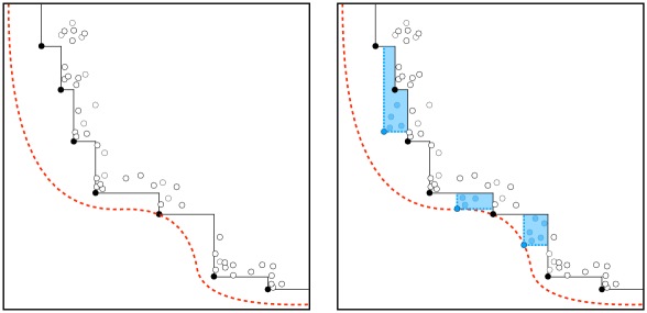
Figure 1: (left) shows true Pareto frontier (red dashed line) and its approximation (black line) based on non-dominated points (black dots), (right) shows updated approximated Pareto frontier based on new non-dominated points (blue dots).

Multi-objective optimization (MOO) problems seek to minimize multiple conflicting objectives $f_{i}:\mathbb{R}^{n}\to\mathbb{R},\forall i\in\left[n_{f}\right]$. Two fundamentally different approaches [HM12] in MOO that deal with this problem are scalarization and the Pareto method, which quantify multi-objective trade-offs a priori and a posteriori, respectively. The weighted sum approach [Zad63] defines the acquisition function $Acq=\sum\nolimits_{i}w_{i}f_{i}(\bm{x})$, representing a scalarization method that combines all objectives into a single objective that is then minimized. This strategy is straightforward to implement and has been applied in other constrained black-box optimization methods [Bey+18]. However, the weighted sum method requires prior knowledge to determine weights $w_{i}$ for different objectives and offers very limited insights into the trade-offs among various competing objectives.

The Pareto method [Par19] seeks to overcome these limitations by exploring the entire Pareto frontier comprised by a set of Pareto-optimal points. By definition, Pareto-optimal points cannot be improved for one objective function without impairing another one. Computing the entire Pareto frontier is expensive and may be infeasible due to limited evaluation budgets. A common way to approximate Pareto frontiers is to instead use “non-dominated” function observations. To give an example, target observation $\bm{Y}_{1}$ is dominated by $\bm{Y}_{2}$ if $Y_{1,j}\geq Y_{2,j},\forall j\in\{1,2,\dots,n_{f}\}$ and $Y_{1,j}>Y_{2,j}$ for at least one $j\in\{1,2,\dots,n_{f}\}$. Fig. 1 shows an example of a two-dimensional Pareto frontier, i.e. when both objectives are being minimized, and its approximated Pareto frontier for a given set of data points and when more data points are added.

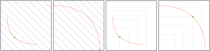
Figure 2: Depicts multi-objective function plot $f_{2}(f_{1}(\bm{x}))$ with Pareto frontier (red line), isocontours of $w=(0.5,0.5)$ scalarization (black lines) and best attainable trade-off based on method used (green dot). (left) convex Pareto frontier using weighted sum approach (middle-left) concave Pareto frontier using weighted sum approach (middle-right) convex Pareto frontier using Chebyshev method (right) concave Pareto frontier using Chebyshev method.

The previously mentioned weighted sum approach can generate certain Pareto frontiers by minimizing the objective functions with varying weights $w_{i}$. However, even in the best case, weighted sums can only reconstruct convex Pareto frontiers [Mes+00]. Fig. 2 visualizes the Pareto method using the weighted sum objective for convex and concave Pareto frontiers and shows the best attainable points.

An alternative approach implementing the Pareto method is the weighted Chebyshev method [Kno06], which defines the objective function as $Acq=\text{max}_{i}\;w_{i}f_{i}$. The weights $w_{i}$ are drawn from a random distribution and defined such that $\sum\nolimits_{i}w_{i}=1$. The choice of distribution can influence what weight combinations the method is focusing on, e.g. using a normal distribution would focus on more equally distributed weights around 0.5. Solving the bilevel optimization problem, i.e. $\text{min}\;Acq=\text{min}\;\text{max}_{i}\;w_{i}f_{i}$, allows reconstruction of Pareto-optimal points on both convex and concave Pareto frontiers. This is visualized in Fig. 2 where we compare the weighted sum and weighted Chebyshev method. The algorithm proposed here utilizes the weighted Chebyshev method in combination with tree ensembles to reveal Pareto-optimal trade-offs of constrained multi-objective optimization problems. The $\epsilon$-constraint method is an alternative way of considering different objectives and has been applied to energy-related problems [Jav+20]. This method minimizes one objective while constraining other objectives to a certain range to generate the Pareto frontier. It is highly effective when there is existing knowledge about some objectives that can be used to determine relevant $\epsilon$ values to constrain these objectives. However, insufficient $\epsilon$ values may produce non-dominated points far away from the true Pareto frontier.

Other approaches that combine prior knowledge of the problem at hand with different data-driven model architectures to determine multi-objective trade-offs are given in [Olo+18, Bey+18]. Another popular class of methods tackling these problems is genetic algorithms (GA) [Kum+10]. One of the most popular algorithms of this category is NSGA-II [Deb+02], which handles constrained multi-objective problems and has been successfully deployed in many energy applications [HF17, MSG20, SH10, VTD15, Yin+14, Zho+16, HN17, Hu+16]. While there is no feasibility guarantee for input constraints, NSGA-II generates solutions that seek to minimize constraint violation. As a state-of-the-art tool with a readily available Python implementation [BD20] that can handle constrained multi-objective optimization problems, we use it as the main method for comparison benchmarks.

3 Method

$f_{i}(\cdot)$	black-box function of objective $i\in\left[n_{f}\right]$
$n$	number of input dimensions
$n_{f}$	number of objectives
$\bm{x}$	variable input vector of size $n$
$\bm{x}^{*}$	optimal input of black-box function $f$
$\bm{x}_{\text{next}}$	next black-box input proposal
$Acq(\cdot)$	acquisition function optimized to determine $\bm{x}_{\text{next}}$
$g(\cdot)$	input equality constraints
$h(\cdot)$	input inequality constraints
$w_{i}$	weight for objective $i$
$\hat{\mu}_{i}(\cdot)$	prediction of tree ensemble for objective $i$
$\alpha(\cdot)$	uncertainty contribution for exploration
$\kappa$	hyperparameter that weights exploration term in acquisition function
$\bm{X}$	input data points $\bm{X}=(\bm{X}_{1},\bm{X}_{2},\dots,\bm{X}_{n})$
$\bm{Y}$	target data points $\bm{Y}=(\bm{Y}_{1},\bm{Y}_{2},\dots,\bm{Y}_{n})$
$\mathcal{N}$	set of continuous variables
$\mathcal{C}$	set of categorical variables
$\mathcal{D}$	available data set
$S_{i}(\cdot,\cdot)$	returns similarity of two data points for categorical feature $i$
$p^{2}(i,j)$	measure of probability for categorical feature $i$ to the take the value $j$
$\mathcal{P}_{a}$	approximated Pareto frontier
$\mathcal{P}_{\text{true}}$	true Pareto frontier

Table 1: General table of notations.

In the following sections we give more details on the proposed method. Section 3.1 outlines the acquisition function used. Sections 3.2 and 3.3 explain the encoding for both tree ensembles and exploration contributions. Table 1 summarizes notations used in the following sections.

3.1 Acquisition Function

We combine the previously mentioned Chebyshev method with the lower confidence bound acquisition function [CJ97], i.e. one of the most popular BO acquisition functions, defined as:

$$Acq(\bm{x})=\hat{\mu}(\bm{x})-\kappa\;\alpha(\bm{x}),$$ (3)

where $\hat{\mu}$ denotes the mean prediction of the surrogate model used. $\alpha$ determines exploration based on an uncertainty metric with $\kappa$ functioning as a hyperparameter to balance the exploitation / exploration trade-off. The combined acquisition function replaces the exploitation part with the Chebyshev approach and uses separate tree ensembles to approximate individual objectives $f_{i}$ with $\hat{\mu}_{i}$:

$$\bm{x}_{\text{next}}\in\underset{\bm{x},\bm{z},\bm{\nu},\hat{\mu},\alpha}{\text{arg min}}\;\underset{i\in\left[n_{f}\right]}{\text{max}}\;\;w_{i}\frac{\hat{\mu}_{i}(\bm{x})-\text{min}(\bm{Y}_{i})}{\text{max}(\bm{Y}_{i})-\text{min}(\bm{Y}_{i})}-\frac{\kappa}{n}\alpha(\bm{x}).$$ (4)

The next black-box evaluation point $\bm{x}_{\text{next}}$ is the result of the bilevel problem stated in Equ. (4). The first term of Equ. (4) comprises the normalized mean function of tree model predictions $\hat{\mu}_{i}$, $i\in\left[n_{f}\right]$, trained on individual target columns multiplied with randomly generated parameters $w_{i}\in\left[0,1\right]$. Note that the normalization of $\hat{\mu}_{i}(\bm{x})$ is only an approximation based on minimum and maximum target observations, i.e. $\text{min}(\bm{Y}_{i})$ and $\text{max}(\bm{Y}_{i})$, in data set $\mathcal{D}$. This allows for the optimization to focus on different parts of the Pareto front depending on which tree model has the largest weight. We emphasize that early iterations are likely going to have poorly normalized objectives, i.e. when the approximated objective bounds are very different to the actual objective bounds. The proposed method allows for users to explicitly specify $\text{min}(\bm{Y}_{i})$ and $\text{max}(\bm{Y}_{i})$ , to avoid poor normalizations of objective values if objective bounds are known a priori. The second term of Equ. (4) is proposed by [The+21] and helps exploration by incentivizing solutions away from previously explored data points. We reformulate optimization objective in Equ. (4) to remove its bilevel nature according to:

$$\bm{x}_{\text{next}}\in \underset{\bm{x},\bm{z},\bm{\nu},\hat{\mu},\alpha}{\text{arg min}}\;\hat{\mu}-\frac{\kappa}{n}\alpha(\bm{x})$$ (5a)

$$\text{s.t.}\;\hat{\mu}\geq w_{i}\frac{\hat{\mu}_{i}(\bm{x})-\text{min}(\bm{Y}_{i})}{\text{max}(\bm{Y}_{i})-\text{min}(\bm{Y}_{i})},\;\forall i\in\left[n_{f}\right]$$ (5b)

Formulations in Equ. (4) and Equ. (5) are equivalent since $\hat{\mu}$ must be greater or equal to all individual tree model contributions. Therefore, at the optimal point, it will be equivalent to the largest tree model prediction, making other tree model contributions redundant.

3.2 Tree Ensemble Encoding

$z_{t,l}$	variable leaf $l$ in tree $t$ acting as a binary variable
$\nu_{i,j}$	binary variable for active split of feature $i$
$v_{i,j}$	numerical value split node $j$ of feature $i$
$v_{i}^{L}$, $v_{i}^{U}$	lower and upper bound of continuous feature $i$
$F_{t,l}$	weight of leaf $l$ in tree $t$
$\mathcal{T}$	set of trees
$\mathcal{L}_{t}$	set of leaves in tree $t$
$\mathbf{splits}(t)$	set of splits of tree $t$
$\mathbf{left}(s)$	leaf indices left of split $s$
$\mathbf{right}(s)$	leaf indices right of split $s$
$\text{V}(s)$	feature participating in split $s$

Table 2: Tree ensemble encoding table of notation.

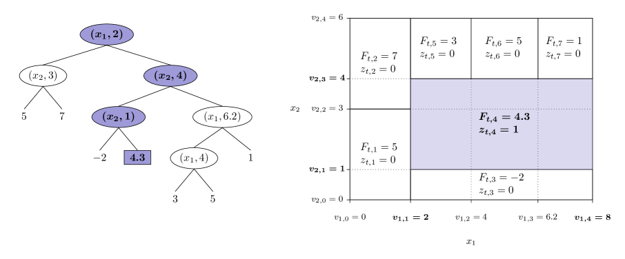
Figure 3: Visualization of a decision tree evaluation.

The proposed method uses the [Miš17] mixed-integer linear programming formulation to encode the tree model [Mis+20]. Tree ensembles are a popular choice for problems with different variable types, i.e. continuous and categorical variables. Continuous variables are defined based on a lower and upper bound, and individual decision trees use splitting conditions to partition the input space. For categorical variables we distinguish between nominal and ordinal variables. For different categories of ordinal variables we can establish an order, but cannot quantify the relative distance between different categories. On the other hand, nominal variables neither define an order nor a distance between different categories. Training a tree ensemble determines split conditions in individual decision trees for different variable types. Table 2 defines the notation in this section. For continuous variables trees define numerical thresholds $v_{i,j}$ as split conditions that determine whether the decision tree evaluation progresses to the left or right branch of the node. The index $i$ indicates the feature involved in the split and $j\in\{1,2,\dots,K_{i}\}$ denotes an ordering for all continuous split conditions in the ensemble according to $v_{i,1}<v_{i,2}<...<v_{i,K_{i}}$. To assign the correct numerical value $v_{i,j}$ to a split $s\in\mathbf{splits}(t)$ in tree $t$ we define $\mathbb{C}(s)=j$ which maps split $s$ onto the correct $j\in\{1,2,\dots,K_{\text{V}(s)}\}$. $\text{V}(s)$ gives the index of the feature participating in split $s$. On the other hand, categorical variables define split conditions as subsets of all possible categories for a feature $i$. LightGBM implements this procedure by grouping for maximum homogeneity as proposed by [Fis58]. With slight abuse of notation, we define $\mathbb{C}(s)\subseteq\{1,2,\dots,K_{\text{V}(s)}\}$ for categorical features. The set $\{1,2,\dots,K_{\text{V}(s)}\}$ has all available categories if $\text{V}(s)$ is a categorical feature. Defining the tree ensemble in this way simplifies the encoding as an optimization model (see Table 2).

We start by defining $\mathcal{N}$ and $\mathcal{C}$ as sets for continuous and categorical variables, respectively. For continuous variables the model defines binary variables $\nu_{i,j}$ corresponding to split condition: $\nu_{i,j}=\mathbb{I}\{x_{i}\leq v_{i,j}\},\forall i\in\mathcal{N},j\in\{1,...,K_{i}\}$. For categorical variables the model defines binary variables $\nu_{i,j}$ corresponding to split condition: $\nu_{i,j}=\mathbb{I}\{x_{i}=j\},\forall i\in\mathcal{C},j\in\{1,...,K_{i}\}$. The following constraints encode the tree model for single objectives according to [Miš17]:

$$\hat{\mu}=\sum\limits_{t\in{\mathcal{T}}}\sum\limits_{l\in{\mathcal{L}_{t}}}F_{t,l}z_{t,l},$$ (6a)

$$\;\;\;\sum\limits_{l\in{\mathcal{L}_{t}}}\;\;\;\;z_{t,l}=1, \forall t\in\mathcal{T},$$ (6b)

$$\sum\limits_{\;\;l\in\mathbf{left}(s)}\;z_{t,l}\leq\sum\limits_{j\in\mathbf{C}(s)}\nu_{\text{V}(s),j}, \forall t\in\mathcal{T},\forall s\in\mathbf{splits}(t),$$ (6c)

$$\sum\limits_{\;\;l\in\mathbf{right}(s)}z_{t,l}\leq 1-\sum\limits_{j\in\mathbf{C}(s)}\nu_{\text{V}(s),j}, \forall t\in\mathcal{T},\forall s\in\mathbf{splits}(t),$$ (6d)

$$\;\;\;\sum\limits_{j=1}^{K_{i}}\;\;\;\nu_{i,j}=1, \forall i\in\mathcal{C},$$ (6e)

$$\nu_{i,j}\leq\nu_{i,j+1}, \forall i\in\mathcal{N},\forall j\in\left[K_{i}-1\right],$$ (6f)

$$\nu_{i,j}\in\{0,1\}, \forall i\in\left[n\right],\forall j\in\left[K_{i}\right],$$ (6g)

$$z_{t,l}\geq 0, \forall t\in{\mathcal{T}},\forall l\in{\mathcal{L}_{t}}.$$ (6h)

For every tree ensemble $\hat{\mu}_{i}$ of Equ. (5), we define the constraints Equ. (6a) as the sum of all active leaf weights $F_{t,l}$, which are obtained from training of the tree ensemble. The leaves are indexed by $t\in{\mathcal{T}}$ and $l\in{\mathcal{L}_{t}}$, with $\mathcal{T}$ and $\mathcal{L}_{t}$ denoting the set of trees and the set of leaves in tree $t$, respectively. Binary variables $z_{t,l}\in\left[0,1\right]$ function as switches indicating which leaves are active. For this model definition [Miš17] shows that variables $z_{t,l}$ can be relaxed to positive continuous variables according to Equ. (6h) without losing their binary behavior, as they are fully-defined by binary variables $\nu_{\text{V}(s),j}$, i.e. Equ. (6c) and Equ. (6d). Relaxing binary variables can allow third party solvers to use more effective solution methods. Equ. (6b) ensures that only one leaf per tree contributes to the tree ensemble prediction. Equ. (6c), (6d) and (6f) force all splits $s\in\mathbf{splits}(t)$, leading to an active leaf, to occur in the correct order. Here $\mathbf{left}(s)$ and $\mathbf{right}(s)$ denote subsets of leaf indices $l\in\mathcal{L}_{t}$ which are left and right of split $s$ in tree $t$. Binary variables $\nu_{\text{V}(s),j}$ determine which splits are active. $\mathbf{C}(s)$ behaves differently depending on the variable type, i.e. continuous or categorical, as previously explained. To ensure that only one of the available categories for feature $i$ is active, Equ. (6e) constraints are added for all categorical variables $i\in\mathcal{C}$. Fig. 3 visualizes the evaluation of a single decision tree and shows which leaf variables are active. For more details on the tree ensemble encoding and theoretical properties of the formulation we refer the reader to [Miš17].
Some key hyperparameters of tree ensembles are the number of trees, the maximum depth of a single decision tree and the minimum number of data points used to define a leaf. While tuning these hyperparameters may improve tree ensemble performance, we assume a pre-defined set of fixed hyperparameter values to allow for a fair comparison with other methods. Standard techniques, e.g. cross-validation or early stopping, could be used to further improve ENTMOOT’s performance and help with exploring unknown areas where model uncertainty is high.

3.3 Search Space Exploration

Next we present details about the Equ. (5) exploration term denoted by $\alpha$. Given that tree ensembles have a piece-wise constant prediction surface with no built-in metric to evaluate uncertainty, we introduce a distance-based exploration measure that incentivizes solutions away from already visited data points. Different strategies to quantify uncertainty for continuous and categorical variables are deployed and combined to define $\alpha$ according to:

$$\alpha\leq\alpha_{\mathcal{N}}^{d}+\alpha_{\mathcal{C}}^{d},\;\;\forall d\in\mathcal{D}$$ (7a)

$$\alpha_{\mathcal{N}}^{d}\in\left[0,|\mathcal{N}|\right]$$ (7b)

$$\alpha_{\mathcal{C}}^{d}\in\left[0,|\mathcal{C}|\right]$$ (7c)

with $\alpha_{\mathcal{N}}^{d}$ and $\alpha_{\mathcal{C}}^{d}$ denoting exploration contributions of continuous and categorical variables, respectively. For continuous variables we define $\alpha_{\mathcal{N}}^{d}$ by introducing distance constraints according to:

$$\alpha_{\mathcal{N}}^{d}\leq\left\lVert\frac{\bm{x}_{\mathcal{N}}-\bm{v}^{L}}{\bm{v}^{U}-\bm{v}^{L}}-\frac{\bm{X}_{d}-\bm{v}^{L}}{\bm{v}^{U}-\bm{v}^{L}}\right\rVert_{2}^{2},\;\;\forall d\in\mathcal{D}$$ (8)

Continuous variable bounds $\bm{v}^{L}$ and $\bm{v}^{U}$ normalize the vector of continuous variables $\bm{x}_{\mathcal{N}}$. Equ. (8) defines $\alpha_{\mathcal{N}}$ as the squared Euclidean distance to the closest normalized data point $\bm{X}_{d}$ and bounds it to $\alpha\in\left[0,1\right]$. Due to the negative contribution of $\alpha$ in Equ. (5), the Equ. (8) quadratic constraints make the overall problem non-convex. These types of non-convex quadratic problems can be solved by commercial branch-and-bound solvers, e.g. Gurobi - v9. The proposed measure is similar to [The+21] and can be reformulated to utilize the standard Euclidean or Manhattan distances. To correlate continuous variables $\bm{x}$ with discrete tree model splits, we introduce linking constraints according to Equ. (9) which assign separate intervals $v_{i,j}$ defined by the tree model splits back to the original continuous search space $\bm{x}\in\mathbb{R}^{n}$. Parameters $v_{i}^{L}$ and $v_{i}^{U}$ denote upper and lower bounds of feature $i$, respectively.

$$x_{i}\geq v^{L}_{i}+\sum\limits_{j=1}^{K_{i}}\left(v_{i,j}-v_{i,j-1}\right)\left(1-\nu_{i,j}\right), \forall i\in\mathcal{N},$$ (9a)

$$x_{i}\leq v^{U}_{i}+\sum\limits_{j=1}^{K_{i}}\left(v_{i,j}-v_{i,j+1}\right)\nu_{i,j}, \forall i\in\mathcal{N},$$ (9b)

$$x_{i}\in\left[v_{i}^{L},v_{i}^{U}\right], \forall i\in\mathcal{N}.$$ (9c)

Quantifying exploration contributions as distances is more difficult when it comes to categorical variables. Here we use similarity measures proposed by [BCK08] that compute the proximity of categorical feature values between two points of the data set. These measures define $S_{i}\left(\bm{X}_{d_{1},i},\bm{X}_{d_{2},i}\right)$ as the similarity between feature $i$ of data points $\bm{X}_{d_{1}}$ and $\bm{X}_{d_{2}}$ with regard to categorical feature $i\in\mathcal{C}$. The easiest way to define $S_{i}$ is the Overlap measure:

$$S_{i}\left(\bm{X}_{d_{1},i},\bm{X}_{d_{2},i}\right)=\begin{cases}1\;\;\bm{X}_{d_{1},i}=\bm{X}_{d_{2},i}\\ 0\;\;\text{otherwise}\end{cases}$$ (10)

Using this measure we observe a range $S_{i}\in\left[0,1\right]$ since it only measures the overlap between categorical features, i.e. having the same category gives similarity of one while having different categorical values give similarity of values. While this measure is easy to implement and effective, it does not take into consideration the number of times different categorical data points already appear in the data set. Here, [BCK08] propose probability based metrics to consider different types of similarities. The property $p^{2}(i,j)$ is a probability estimate of category $j$ of feature $i$ appearing in data set $\mathcal{D}$ and is defined as:

$$p^{2}\left(i,j\right)=\frac{\text{count}_{i}\left(j\right)\left(\text{count}_{i}\left(j\right)-1\right)}{\mid\mathcal{D}\mid\left(\mid\mathcal{D}\mid-1\right)}$$ (11)

Large values of $p^{2}(i,j)$ indicate a high probability that categorical feature $i$ will have the value $j$. [BCK08] use $p^{2}(i,j)$ to define the Goodall4 similarity according to

$$S_{i}\left(\bm{X}_{d_{1},i},\bm{X}_{d_{2},i}\right)=\begin{cases}p^{2}\left(i,\bm{X}_{d_{1},i}\right)&\text{if}\;\bm{X}_{d_{1},i}=\bm{X}_{d_{2},i}\\ 0&\text{otherwise}\end{cases}$$ (12)

For categorical variables we link the distance metric to the exploration term by adding the following constraints to our optimization problem:

$$\alpha_{\mathcal{C}}^{d}\leq\sum\limits_{i\in\mathcal{C}}\sum\limits_{j=1}^{K_{i}}\left[1-S_{i}\left(\bm{X}_{d,i},j\right)\right]\nu_{i,j},\;\;\forall d\in\mathcal{D}$$ (13)

Equ. (12) computes larger similarities for features that occur more often in the data set, causing $\alpha_{\mathcal{C}}^{d}$ in Equ. (13) to take smaller values, which incentivizes solutions that appear less frequently in data set $\mathcal{D}$. We can read active categorical variable values by checking which of the $\nu_{i,j}$ binary variables is not zero:

$$x_{i}=\underset{j\in\left[K_{i}\right]}{\text{argmax}}\;\{\nu_{i,j}\},\forall i\in\mathcal{C}.$$ (14)

We note that Equ. (14) is not part of the optimization problem and should demonstrate how active labels are linked to $\bm{x}_{\text{next}}$. In summary, the resulting optimization model that determines the next promising input $\bm{x}_{\text{next}}$ uses Equ. (5), Equ. (6) for every tree model, Equ. (8), Equ. (9) and Equ. (13), and is classified as a mixed-integer non-convex quadratic problem.

3.4 Combined Model

The combined model consists of the Section 3.2 tree ensemble encodings and the Section 3.3 exploration measure. The proposed method uses the modified Chebyshev method introduced in Section 3.1. Optimization of the tree model encoding is an NP-hard problem [Miš17], and, together with the exploration measure, can be classified as a nonconvex mixed-integer quadratic program. The nonconvex part originates from the definition of $\alpha_{\mathcal{N}}^{d}$ as a quadratic in Equ. (8), which is then maximized in the objective function, i.e. its negative value is minimized. While these formulations do not scale well with growing problem sizes, [The+21] found that most problems converge within minutes due to the usage of effective heuristics in third party solvers. [Miš17], [The+21] and [Mis+20] also propose custom heuristics specifically tailored for optimization problems including tree ensembles to enhance bound improvement when optimizing such models.
The tree encoding defined in Equ. (6) adds constraints for splits in every decision tree and scales with the size of the tree ensemble. While it is independent of the number of data points and the dimensionality, one would expect larger tree ensembles for large data sets and high-dimensional spaces, and therefore more constraints in the optimization model. The uncertainty metric defined in Section 3.3 directly scales with the size of the data set, dimensionality as well as number of categories if categorical variables are involved. Equ. (7) and Equ. (8) are added for every additional data point, and the vectors in Equ. (8) grow with increasing dimensionality, making the resulting problem more difficult to solve. Moreover, similarity matrix $S$ for categorical variables grows with increasing number of data points and Equ. (13) is added for every data point. [The+21] solve a similar problem for single objective problems and propose using data clustering to combine multiple data points into single cluster centers to reduce the size of the problem. While the proposed method is inherently difficult to solve, we motivate its usefulness by empirically evaluating it on practically motivated case studies. The superior performance with respect to sampling efficiency of the proposed method motivates its usage over cheaper algorithms, e.g.NSGA-II, especially when black-box functions are expensive to evaluate.

4 Numerical Studies

This section empirically evaluates the framework proposed in this paper. Code recapitulating the ENTMOOT results can be found here: https://github.com/cog-imperial/moo_trees. We select synthetic benchmarks with known Pareto fronts that enable comprehensive comparison with respect to performance metrics. Moreover, we present two practically motivated case studies, i.e., wind turbine placement (WTP) and battery material selection (BMS), that emphasize the advantages of the proposed method and highlight its relevance to energy systems. For all studies we assume expensive black-box evaluations comprise the majority of the total computational complexity of each run. Therefore, we evaluate solver performance based on how many black-box evaluations are needed to explore the Pareto frontier, i.e. different metrics are used to measure the progress. For all experiments we provide medians for all performance metrics, as well as first and third quartiles that bound the confidence intervals, computed using 25 runs with ordered random seeds in $\{101,102,...125\}$. The same set of initial points are provided for all competing methods to facilitate comparison. By using the same set of initial data points and testing multiple random seeds, we mitigate the effects of specific initial settings favoring one method over the other. For the case studies with unknown Pareto frontiers we compute the bounded hypervolume of the objective space over number of black-box evaluations. The number of black-box evaluations contributes to the overall computational complexity, and we therefore compare methods based on how many black-box evaluations are needed to improve the bounded hypervolume of the objective space.
We compare the proposed methods to NSGA-II using its pymoo [BD20] implementation. Additionally, we investigate random search for unconstrained problems using a feasible sampling strategy, as described in Section 4.3.2. The NSGA-II method is used with default hyperparameter values in pymoo, except for initial population size, which is set consistently with the other considered methods. Since NSGA-II does not directly support categorical variables, we apply one-hot encoding by introducing continuous auxiliary variables for all categories of a categorical variable bounded within $\left[0.0,1.0\right]$. The auxiliary variable with the highest numerical value determines the category picked. ENTMOOT uses 400 trees with a maximum tree depth of three and a minimum of two data points per leaf. The tree ensemble is trained using LightGBM [Ke+17], and the default value of $\kappa=1.96$ is picked for all numerical studies. To allow for a fair comparison with other methods, we used the same set of hyperparameters for ENTMOOT throughout all runs. ENTMOOT uses Gurobi - v9 to solve the mixed-integer quadratic program (MIQP) with default parameter settings to find minima of the tree ensemble surrogate model. We found that for most instances Gurobi - v9 finds a global optimal solution in a fairly short time given the default relative optimality gap of $1\text{\times}{10}^{-4}$ and feasibility tolerance of $1\text{\times}{10}^{-6}$. However, sometimes Gurobi - v9 struggles to fully close the optimality gap, so we enforce a time limit of 100 s, given that a feasible solution is found, due to computational limitations when running batch jobs. If a feasible solution is not found, the optimization procedure is continued until one is found. We note that this procedure only affects the method presented here, and not other tools that we compare against. All experiments are run on a Linux machine equipped with an Intel Core i7-7700K 4.20 GHz and 16 GB of memory.

4.1 Performance Metrics

We use multiple different measures to compare the performance of different algorithms. For benchmarks where the true Pareto frontier is known, we rely on the Euclidean generational distance (GD) [Van99], the inverted generational distance (IGD) [SC04], the maximum Pareto frontier error (MPFE) [Van99] and the volume ratio (VR) [Olo+18]. The true Pareto frontier is denoted as $\mathcal{P}_{\text{true}}$ and $\mathcal{P}_{a}$ is the approximated Pareto frontier derived by different algorithms. For synthetic benchmarks in Section 4.2, $\mathcal{P}_{\text{true}}$ is determined by running NSGA-II for a few thousand iterations. For energy systems related benchmarks there is no true Pareto frontier available, and we compare the hypervolume bounded by the approximate Pareto frontiers derived from different algorithms.

We compute GD according to:

$$\text{GD}\left(\mathcal{P}_{a}\right)=\frac{1}{|\mathcal{P}_{a}|}\sum\limits_{\bm{r}\in\mathcal{P}_{a}}\underset{\bm{r}^{\left(t\right)}\in\mathcal{P}_{\text{true}}}{\text{min}}\;\left\lVert\bm{r}-\bm{r}^{\left(t\right)}\right\rVert_{2},$$ (15)

which describes the average distance of points in in the approximated Pareto frontier $\mathcal{P}_{a}$ to the true Pareto frontier $\mathcal{P}_{\text{true}}$. The results of this measure may be misleading if the approximate number consists of only a few good Pareto points. To overcome this problem we also report IGD which computes the average distance of points on the true Pareto frontier to the approximate Pareto frontier according to:

$$\text{IGD}\left(\mathcal{P}_{a}\right)=\frac{1}{|\mathcal{P}_{\text{true}}|}\sum\limits_{\bm{r}^{\left(t\right)}\in\mathcal{P}_{\text{true}}}\underset{\bm{r}\in\mathcal{P}_{a}}{\text{min}}\;\left\lVert\bm{r}^{\left(t\right)}-\bm{r}\right\rVert_{2}.$$ (16)

The MPFE measure is defined as:

$$\text{MPFE}\left(\mathcal{P}_{a}\right)=\underset{\bm{r}^{\left(t\right)}\in\mathcal{P}_{\text{true}}}{\text{max}}\;\underset{\bm{r}\in\mathcal{P}_{a}}{\text{min}}\;\left\lVert\bm{r}-\bm{r}^{\left(t\right)}\right\rVert_{2},$$ (17)

and computes the maximum error of the approximate Pareto frontier to the true Pareto frontier. The MPFE measure can be sensitive to outliers, since a single bad point on Pareto frontier is sufficient to negatively influence the measure. VR is a measure that takes the entirety of the approximated Pareto frontier into consideration:

$$\text{VR}\left(\mathcal{P}_{a}\right)=-\log{\left(1-\frac{\text{Vol}\left(\mathcal{P}_{a}\right)}{\text{Vol}\left(\mathcal{P}_{\text{true}}\right)}\right)}$$ (18)

with $\text{Vol}(\cdot)$ describing the hypervolume of the Pareto frontier. The VR measure computes the ratio of hypervolume bounded by the approximate Pareto frontier vs. the hypervolume bounded by the true Pareto frontier. We note that the VR measure is undefined if $\mathcal{P}_{a}$ exactly matches $\mathcal{P}_{\text{true}}$. However, since $\mathcal{P}_{\text{true}}$ itself is an approximation of the true Pareto frontier as stated above, this case is highly unlikely. The Equ. (18) logarithm helps distinguish solutions with $\text{Vol}\left(\mathcal{P}_{a}\right)\ /\text{Vol}\left(\mathcal{P}_{\text{true}}\right)\simeq 1$, e.g. improvements of $\text{Vol}\left(\mathcal{P}_{a}\right)\ /\text{Vol}\left(\mathcal{P}_{\text{true}}\right)$ from 99 % to 99.9 % are valued higher than increasing the ratio from 19 % to 19.9 %.

4.2 Synthetic Benchmarks

We test the proposed method on various synthetic benchmarks to show its competitive performance compared to other state-of-the-art methods. The synthetic benchmarks provided in this section have different types of Pareto frontiers to show the algorithm’s capability of reproducing them and each have two objective functions. The Fonzeca & Fleming problem [FF95] is a popular choice for benchmarking multi-objective optimization frameworks and is defined as:

$$\begin{cases}f_{1}(\bm{x})=1-\text{exp}\left(-\sum\limits_{i=1}^{D}\left(x_{i}-\frac{1}{\sqrt{D}}\right)^{2}\right),\\ f_{2}(\bm{x})=1-\text{exp}\left(-\sum\limits_{i=1}^{D}\left(x_{i}+\frac{1}{\sqrt{D}}\right)^{2}\right).\end{cases}$$ (19)

Fig. 4 shows the concave Pareto frontier of the function. The function inputs $x_{i}\in\left[-4,4\right]$ for $i\in\{1,2,\dots,D\}$ bound the function outputs according to $f_{1}(\bm{x}),f_{2}(\bm{x})\in\left[0,1\right]$. For our tests we choose $D=2$.

The second synthetic benchmark function is Schaffer [Sch85] given by:

$$\begin{cases}f_{1}(\bm{x})=x^{2},\\ f_{2}(\bm{x})=(x-2)^{2}.\end{cases}$$ (20)

Schaffer has a convex Pareto frontier as depicted in Fig. 4. Inputs of Schaffer are defined as $x\in\left[-3,3\right]$ bounding the objectives according to $f_{1}(x)\in\left[0,9\right]$ and $f_{2}(x)\in\left[0,25\right]$.

Kursawe [Kur90] is the third benchmark function which we use for comparison. The Kursawe function is interesting due to its discontinuous Pareto frontier and is defined as:

$$\begin{cases}f_{1}(\bm{x})=\sum\limits_{i=1}^{D-1}\left[-10\text{exp}\left(-0.2\sqrt{x_{i}^{2}+x_{i+1}^{2}}\right)\right],\\ f_{2}(\bm{x})=\sum\limits_{i=1}^{D}\left[|x_{i}|^{0.8}+5\sin{\left(x_{i}^{3}\right)}\right]\end{cases}$$ (21)

Kursawe has inputs defined as $x_{i}\in\left[-5,5\right]$ for $i\in\{1,2,\dots,D\}$ with $D=3$. Approximate output bounds for Kursawe are given as $f_{1}(\bm{x})\in\left[-20,-4\right]$ and $f_{2}(\bm{x})\in\left[-12,25\right]$.

We also include the $\text{S}^{+}$ and $\text{S}^{-}$ benchmark from [Olo+18] to test the proposed algorithm on a problem that has both convex and concave sections on the Pareto frontier. The functions are defined as follows:

$$\begin{cases}f_{1}(\bm{x})=x_{1},\\ f_{2}(\bm{x})=10-x_{1}+x_{2}\pm\sin\left(x_{1}\right)\end{cases}$$ (22)

where $\text{S}^{+}$ and $\text{S}^{-}$ are differentiated by the sign of the sinusoidal function in $f_{2}$. The two-dimensional inputs for both functions are given as $x_{1}\in\left[0,10\right]$ and $x_{2}\in\left[0,10\right]$. The approximate bounds of both objectives are $f_{1}(\bm{x})\in\left[0,10\right]$ and $f_{2}(\bm{x})\in\left[-1,12\right]$.

Based on preliminary studies we found that the performance of different algorithms is highly dependent on the quality of the initial population. Therefore, we provide the same randomly sampled ten initial points to all methods for the synthetic benchmarks.

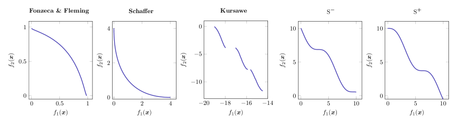
Figure 4: Pareto frontiers of synthetic benchmark functions.

Table 3 presents the results of all synthetic benchmark tests. The average of all random seeds for the proposed tree-based surrogate model outperforms NSGA II and random-search on all of the benchmark problems after 80 iterations for GD, IGD and VR metrics. For the MPFE metric the proposed method wins for every synthetic function except the Kursawe function. The results highlight the sampling-efficiency of surrogate-based methods.

		GD ($\times 100$)		inv. GD ($\times 100$)		MPFE		VR
Problem	Itr	ENTMOOT	NSGA2 / rnd	ENTMOOT	NSGA2 / rnd	ENTMOOT	NSGA2 / rnd	ENTMOOT	NSGA2 / rnd
	10	37.65 $\pm$ (7.7)	37.65 $\pm$ (7.7)	4.15 $\pm$ (0.5)	4.15 $\pm$ (0.5)	0.95 $\pm$ (0.1)	0.95 $\pm$ (0.1)	0.03 $\pm$ (0.1)	0.03 $\pm$ (0.1)
Fonzeca &	20	16.90 $\pm$ (7.1)	24.00 $\pm$ (7.8)	2.93 $\pm$ (0.6)	3.59 $\pm$ (0.6)	0.67 $\pm$ (0.1)	0.89 $\pm$ (0.1)	0.42 $\pm$ (0.2)	0.10 $\pm$ (0.2)
Fleming [FF95]	40	4.09 $\pm$ (1.4)	10.93 $\pm$ (7.7)	1.51 $\pm$ (0.4)	2.83 $\pm$ (0.6)	0.45 $\pm$ (0.1)	0.77 $\pm$ (0.2)	1.47 $\pm$ (0.3)	0.51 $\pm$ (0.3)
	60	2.20 $\pm$ (0.4)	5.89 $\pm$ (6.4)	1.10 $\pm$ (0.4)	2.01 $\pm$ (0.6)	0.38 $\pm$ (0.2)	0.55 $\pm$ (0.1)	2.10 $\pm$ (0.4)	0.78 $\pm$ (0.4)
	80	1.48 $\pm$ (0.4)	4.33 $\pm$ (4.8)	0.87 $\pm$ (0.4)	1.55 $\pm$ (0.5)	0.30 $\pm$ (0.2)	0.41 $\pm$ (0.1)	2.54 $\pm$ (0.5)	1.29 $\pm$ (0.4)
	10	25.66 $\pm$ (20.7)	25.66 $\pm$ (20.7)	1.80 $\pm$ (0.5)	1.80 $\pm$ (0.5)	1.56 $\pm$ (0.3)	1.56 $\pm$ (0.3)	2.75 $\pm$ (0.7)	2.75 $\pm$ (0.7)
Schaffer [Sch85]	20	5.86 $\pm$   (3.3)	7.54 $\pm$   (9.7)	1.00 $\pm$ (0.1)	1.37 $\pm$ (0.4)	0.90 $\pm$ (0.2)	1.11 $\pm$ (0.2)	4.61 $\pm$ (0.4)	3.69 $\pm$ (0.6)
	40	1.24 $\pm$   (0.9)	1.58 $\pm$   (2.4)	0.65 $\pm$ (0.1)	0.85 $\pm$ (0.3)	0.65 $\pm$ (0.2)	0.81 $\pm$ (0.2)	5.63 $\pm$ (0.5)	4.65 $\pm$ (0.6)
	60	0.69 $\pm$   (0.3)	0.92 $\pm$   (1.2)	0.53 $\pm$ (0.1)	0.67 $\pm$ (0.2)	0.58 $\pm$ (0.2)	0.64 $\pm$ (0.2)	6.16 $\pm$ (0.6)	5.46 $\pm$ (0.5)
	80	0.52 $\pm$   (0.2)	0.59 $\pm$   (0.2)	0.45 $\pm$ (0.1)	0.54 $\pm$ (0.1)	0.51 $\pm$ (0.2)	0.56 $\pm$ (0.1)	6.53 $\pm$ (0.7)	5.85 $\pm$ (0.4)
	10	177.12 $\pm$ (32.6)	177.12 $\pm$ (32.6)	21.15 $\pm$ (3.0)	21.15 $\pm$ (3.0)	3.23 $\pm$ (0.3)	3.23 $\pm$ (0.3)	0.55 $\pm$ (0.2)	0.55 $\pm$ (0.2)
Kursawe [Kur90]	20	136.79 $\pm$ (25.1)	136.20 $\pm$ (23.2)	20.08 $\pm$ (2.9)	18.98 $\pm$ (2.6)	3.03 $\pm$ (0.3)	2.88 $\pm$ (0.3)	0.83 $\pm$ (0.2)	0.73 $\pm$ (0.2)
	40	61.70 $\pm$ (22.1)	94.14 $\pm$ (18.4)	13.84 $\pm$ (1.9)	17.30 $\pm$ (2.6)	2.47 $\pm$ (0.3)	2.58 $\pm$ (0.3)	1.41 $\pm$ (0.2)	0.99 $\pm$ (0.2)
	60	32.17 $\pm$ (11.6)	78.84 $\pm$ (20.0)	12.37 $\pm$ (2.1)	14.74 $\pm$ (2.8)	2.43 $\pm$ (0.3)	2.39 $\pm$ (0.3)	1.65 $\pm$ (0.2)	1.23 $\pm$ (0.3)
	80	23.62 $\pm$   (8.2)	57.72 $\pm$ (21.0)	10.71 $\pm$ (2.6)	13.14 $\pm$ (2.4)	2.33 $\pm$ (0.4)	2.22 $\pm$ (0.3)	1.77 $\pm$ (0.3)	1.41 $\pm$ (0.3)
	10	27.41 $\pm$ (5.0)	27.41 $\pm$ (5.0)	3.49 $\pm$ (0.4)	3.49 $\pm$ (0.4)	1.77 $\pm$ (0.3)	1.77 $\pm$ (0.3)	1.41 $\pm$ (0.2)	1.41 $\pm$ (0.2)
S+ [Olo+18]	20	17.18 $\pm$ (2.8)	19.14 $\pm$ (3.6)	2.77 $\pm$ (0.2)	2.85 $\pm$ (0.4)	1.41 $\pm$ (0.1)	1.40 $\pm$ (0.3)	1.90 $\pm$ (0.2)	1.92 $\pm$ (0.2)
	40	10.12 $\pm$ (1.0)	13.73 $\pm$ (2.7)	2.10 $\pm$ (0.2)	2.24 $\pm$ (0.3)	1.08 $\pm$ (0.2)	1.21 $\pm$ (0.2)	2.26 $\pm$ (0.3)	2.29 $\pm$ (0.2)
	60	7.27 $\pm$ (0.9)	10.69 $\pm$ (2.6)	1.76 $\pm$ (0.1)	2.08 $\pm$ (0.2)	0.96 $\pm$ (0.1)	1.06 $\pm$ (0.2)	2.60 $\pm$ (0.4)	2.47 $\pm$ (0.2)
	80	5.24 $\pm$ (0.5)	8.37 $\pm$ (2.5)	1.57 $\pm$ (0.1)	1.92 $\pm$ (0.1)	0.88 $\pm$ (0.1)	1.01 $\pm$ (0.1)	2.78 $\pm$ (0.4)	2.73 $\pm$ (0.2)
	10	27.93 $\pm$ (3.8)	27.93 $\pm$ (3.8)	3.26 $\pm$ (0.2)	3.26 $\pm$ (0.2)	1.65 $\pm$ (0.2)	1.65 $\pm$ (0.2)	1.35 $\pm$ (0.2)	1.35 $\pm$ (0.2)
S- [Olo+18]	20	18.12 $\pm$ (1.9)	19.56 $\pm$ (2.6)	2.61 $\pm$ (0.2)	2.68 $\pm$ (0.2)	1.31 $\pm$ (0.1)	1.30 $\pm$ (0.2)	1.92 $\pm$ (0.1)	1.81 $\pm$ (0.1)
	40	10.35 $\pm$ (1.2)	13.73 $\pm$ (2.3)	2.02 $\pm$ (0.1)	2.29 $\pm$ (0.2)	1.10 $\pm$ (0.1)	1.14 $\pm$ (0.1)	2.55 $\pm$ (0.1)	2.15 $\pm$ (0.1)
	60	7.40 $\pm$ (0.7)	10.39 $\pm$ (2.5)	1.68 $\pm$ (0.1)	2.08 $\pm$ (0.1)	0.97 $\pm$ (0.1)	1.05 $\pm$ (0.1)	2.93 $\pm$ (0.1)	2.35 $\pm$ (0.1)
	80	5.38 $\pm$ (0.5)	8.17 $\pm$ (2.3)	1.51 $\pm$ (0.1)	1.95 $\pm$ (0.1)	0.89 $\pm$ (0.1)	1.00 $\pm$ (0.1)	3.21 $\pm$ (0.1)	2.49 $\pm$ (0.1)

Table 3: Results of synthetic benchmark problems comparing ENTMOOT against the best result of NSGA-II and random-search based on different performance metrics. Each entry shows the Median of all runs with different random seeds and the standard deviation in brackets after a certain amount of black-box evaluations with winning median highlighted in bold.

4.3 Optimization of Windfarm Layout

$u_{j}$	experienced velocity of turbine $j$
$u_{0}$	ambient wind speed
$u_{k,j}$	interference caused on turbine $j$ by turbine $k$
$C_{T,k}$	thrust coefficient of $k$-th turbine at given windspeed
$A_{j}$	rotor area of $j$-th turbine
$A_{k,j}$	rotor area of $j$-th turbine lying in the wake of turbine $k$
$h_{\text{hub}}$	turbine hub height
$z_{0}$	surface roughness height
$\text{dist}_{k,j}$	distance between turbines $k$ and $j$
$\xi$	degree of wake expansion
$R_{k}$	radius of wind turbine $k$
$c_{k,j}$	distance from turbine $j$ to center of wake from turbine $k$ when it reaches turbine $j$
$f_{w}$	annual frequency at which certain wind speeds occur
$P_{j}(\cdot)$	power generated by turbine $j$
$P_{j}^{\text{ideal}}(\cdot)$	power generated by turbine $j$ without wake effects
$x_{\text{turb}},k$	x-coordinates of turbine $k$
$y_{\text{turb}},k$	y-coordinates of turbine $k$
$b_{k}$	binary variable indicating if turbine $k$ is active
$b_{k,j}^{\text{dist}}$	auxiliary binary variable indicating if distance constrained for turbines $k$ and $j$ is active
$\text{dist}_{k,j}$	continuous variable for distance between turbines $k$ and $j$, change with definition above
$\alpha_{\text{samp}}$	continuous variable that gives maximum distance to closest sampling point
$k_{i}^{d,+}$	auxiliary variable takes positive contribution of Manhattan distance between $x_{i}$ and data point $d$
$k_{i}^{d,-}$	auxiliary variable takes negative contribution of Manhattan distance between $x_{i}$ and data point $d$
$N_{\text{turb}}$	number of active turbines

Table 4: Wind turbine benchmark table of notation.

4.3.1 General Model Description

In this section, we consider the optimal layout of an offshore windfarm based on the model by [RBB16]. In general, formulations for optimization of windfarm layouts can be nonlinear, multi-modal, non-differentiable, non-convex, and discontinuous, making them difficult to solve using model-based optimization techniques. Therefore, the resulting problems are often solved using multi-objective black-box optimization schemes. We note that, while the model presented here is based on several simplifications, the proposed optimization strategy is general and can be applied to more complicated windfarm models, including those that cannot be expressed analytically.

The placement of wind turbines is complicated by wake effects, or the effect of one turbine on the power generation of another. Wake losses are approximated using the model by [KHJ86], which provides a simple model for approximating wind velocity in the wake of some turbine(s). Table 4 provides the notation for this case study.

Following this model, the velocity experienced by the $j$-th turbine is expressed:

$$u_{j}=u_{0}(1-\sqrt{\sum_{k\neq j}u_{k,j}^{2}})$$ (23)

where $u_{0}$ is the ambient wind speed (without wake effects) and $u_{k,j}$ is the interference caused on turbine $j$ by turbine $k$. The pairwise interference terms are calculated as:

$$u_{k,j} =\frac{1-\sqrt{1-C_{T,k}}}{(1+\xi\text{dist}_{k,j}/R_{j})^{2}}\frac{A_{k,j}}{A_{j}}$$ (24)

$$\xi =0.5\mathrm{log}^{-1}\left(\frac{h_{\mathrm{hub}}}{z_{0}}\right)$$ (25)

where $C_{T,k}$ is the thrust coefficient of the $k$-th turbine at a given windspeed, $A_{j}$ is the rotor area of the $j$-th turbine, and $A_{k,j}$ is the rotor area of the $j$-th turbine that lies in the wake of turbine $k$. The variable $\text{dist}_{k,j}$ denotes distance between turbines $k$ and $j$, and $\xi$ represents the degree of wake expansion, computed using turbine hub height $h_{\mathrm{hub}}=107$ m, and surface roughness height $z_{0}$, assumed to be $5\times 10^{-4}$ m. It is further assumed that the wake of each turbine expands linearly, i.e., $R_{k,j}=R_{k}+\xi\text{dist}_{k,j}$, where $R_{k}$ is the radius of the turbine rotor. Therefore, the rotor area of turbine $j$ in the wake of turbine $k$, $A_{k,j}$, can be computed as:

$$A_{k,j}=\frac{1}{2}\left(R_{k,j}^{2}\left(2\mathrm{arccos}\left(\frac{R_{k,j}^{2}+c_{k,j}^{2}-R_{j}^{2}}{2R_{k,j}c_{k,j}}\right)-\mathrm{sin}\left(2\mathrm{arccos}\left(\frac{R_{k,j}^{2}+c_{k,j}^{2}-R_{j}^{2}}{2R_{k,j}c_{k,j}}\right)\right)\right)\right)+\\ \frac{1}{2}\left(R_{j}^{2}\left(2\mathrm{arccos}\left(\frac{R_{j}^{2}+c_{j,k}^{2}-R_{k,j}^{2}}{2R_{j}c_{j,k}}\right)-\mathrm{sin}\left(2\mathrm{arccos}\left(\frac{R_{j}^{2}+c_{k,j}^{2}-R_{k,j}^{2}}{2R_{j}c_{j,k}}\right)\right)\right)\right)$$ (26)

where $c_{k,j}$ is the distance from turbine $j$ to the center of the wake from turbine $k$ when it reaches turbine $j$. Note that if the wake front entirely covers turbine $j$, then instead $A_{k,j}$ is set to $\pi R_{j}^{2}$, and if the wake front does not impact turbine $j$, then $A_{k,j}=0$.

Wind turbines are assumed to be identical “Vestas 8 MW” units, whose power and thrust curves are linearly interpolated and given in [RBB16]. Each turbine has a rotor radius of 82 m. We further use the discretized North Sea wind distribution data from [RBB16]. This application places the base of up to 16 wind turbines within a square 15.21 $\text{km}^{2}$ area based on optimal tradeoffs of two conflicting objectives to explore the Pareto frontier. We represent the coordinates of each turbine using two continuous variables; therefore, the degrees of freedom for the windfarm problem $\bm{x}$ comprise 32 positive continuous variables, i.e. Equ. (28f) and Equ. (28g), denoting the location of each of the 16 wind turbines. Furthermore, 16 binary variables, i.e. Equ. (6e), are introduced to indicate which wind turbines are active.

Optimization of the windfarm layout involves two objective functions:

$$\begin{cases}f_{1}(\bm{x})=\frac{\sum_{w}\sum_{j=1}^{16}P_{j}(u_{w})f_{w}}{\sum_{w}16P_{j}^{\mathrm{ideal}}(u_{w})f_{w}},\\ f_{2}(\bm{x})=\frac{\sum_{w}\sum_{j=1}^{16}P_{j}(u_{w})f_{w}}{N_{\text{turb}}P_{j}^{\mathrm{ideal}}}.\end{cases}$$ (27)

where $P_{j}(u_{w})$ is the power generated by turbine $j$ generated at wind velocity $u_{w}$ (wind data is discretized in to winds with velocity $u_{w}$ and frequency $f_{w}$). $P_{j}^{\mathrm{ideal}}(u_{w})$ is the power generated by turbine $j$ at wind velocity $u_{w}$ without any wake effects, and $N_{\text{turb}}$ is the number of turbines placed in the farm. The objectives $f_{1}$ and $f_{2}$ correspond to the energy production and efficiency, respectively. The two objectives represent conflicting design goals, as production is increased by placing more turbines in the wind farm. However, wake effects also increase with the number of turbines, decreasing the windfarm efficiency.

4.3.2 Optimization Benchmark

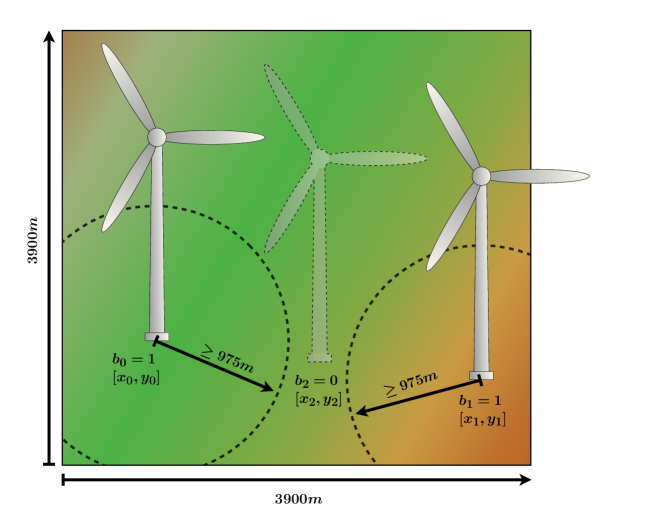
Figure 5: Example for feasible layout using three wind turbines visualizing optimization variables from Equ. (28). Variabels $b$ indicate if a wind turbine is active and $[x,y]$ give its coordinates. Circles around wind turbines indicate the Equ. (28b) minimum distance constraints of 975 m between individual wind turbines.

For the windfarm benchmark we distinguish between required and supporting constraints, i.e. Equ. (28) and Equ. (29), respectively. Required constraints are given by the problem description and must be satisfied by feasible solutions. Equ. (28b) define auxiliary variables $\text{dist}_{i,j}$ as the distance between two wind turbine locations and Equ. (28c) defines the minimum of distance $\text{dist}_{k,j}$ as 975 m when both turbines $k$ and $j$ are active which is given when Equ. (28d) is zero. Fig. 5 depicts a feasible layout for three wind turbines. Moreover, supporting constraints in Equ. (29) are added to break symmetry and remove equivalent solutions. Equ. (29a) assures that wind turbines are activated in an increasing order, e.g. for the case that two wind turbines are active this allows only for binary variables $b_{1}$ and $b_{2}$ to be active. The inequality constraints Equ. (29b) and Equ. (29c) enforce a default location of $(0,0)$ for inactive wind turbines since their location has no influence on the black-box objective. We found that NSGA-II struggles to consistently provide feasible solutions for the required constraints in Equ. (28), so we exclude supporting constraints from Equ. (29) because they further restrict the search space. Since ENTMOOT and the initial sampling set both provide guaranteed $\epsilon$-feasible solutions, additional supporting constraints from Equ. (29) can be added to further limit the search space and prevent the algorithm from finding redundant solutions.
Required Constraints

$$\sum\limits_{k=1}^{|\bm{b}|}b_{k}\geq 1,$$ (28a)

$$\text{dist}_{k,j}^{2}\leq\left(x_{\text{turb},k}-x_{\text{turb},j}\right)^{2}+\left(y_{\text{turb},k}-y_{\text{turb},j}\right)^{2}, \forall k\in\left[1,...,16\right],\;\forall j\in\left[k+1,...,16\right]$$ (28b)

$$b_{k,j}^{\text{dist}}\rightarrow\text{dist}_{i,j}\geq 975, \forall k\in\left[1,...,16\right],\;\forall j\in\left[i+1,...,16\right],$$ (28c)

$$b_{k,j}^{\text{dist}}=b_{k}\cdot b_{j}, \forall k\in\left[1,...,16\right],\;\forall j\in\left[k+1,...,16\right],$$ (28d)

$$\bm{b}\in\left\{0,1\right\}^{16},$$ (28e)

$$\bm{x}_{\text{turb}}\in\left[0.0,3900.0\right]^{16},$$ (28f)

$$\bm{y}_{\text{turb}}\in\left[0.0,3900.0\right]^{16}$$ (28g)

$$\text{dist}_{k,j}\in\mathbb{R}^{\text{+}}, \forall k\in\left[1,...,16\right],\;\forall j\in\left[k+1,...,16\right]$$ (28h)

$$b_{k,j}^{\text{dist}}\in\left\{0,1\right\}, \forall k\in\left[1,...,16\right],\;\forall j\in\left[k+1,...,16\right].$$ (28i)

Helper Constraints

$$b_{k}\geq b_{k+1}, \forall k\in\left[1,...,15\right],$$ (29a)

$$\neg b_{i}\rightarrow x_{\text{turb},k}\leq 0, \forall k\in\left[1,...,16\right],$$ (29b)

$$\neg b_{i}\rightarrow y_{\text{turb},k}\leq 0, \forall k\in\left[1,...,16\right].$$ (29c)

We use an advanced initialisation strategy to ensure that only feasible initial populations are provided for both ENTMOOT and NSGA-II. Moreover, the solutions are created for fixed numbers of wind turbines. The goal is to provide 16 initial solutions with $1,2,...,16$ wind turbines to expose both tested algorithms to initial points that contain all possible numbers of wind turbines. The algorithm to compute the initial set of data points $\mathcal{D}_{\text{init}}$ is given as Algorithm 1. The first data point has one turbine placed at the middle of the field with random noise $\epsilon_{\text{noise}}$ added to the its position to get varying results for different random seeds. Equ. (30) takes into consideration all data points that are currently in $\mathcal{D}_{\text{init}}$ and maximizes the Manhattan distance to the closest sample that is available. We encode the Manhattan distance according to [GP02]. Equ. (30c) enforces $k_{i}^{d,+}$ and $k_{i}^{d,-}$ to take positive and negative values of the difference between $x_{i}$ and the closest data point, respectively. Equ. (6d) is implemented using special ordered sets [Tom88] to assure that at least one of the variables $k_{i}^{d,+}$ and $k_{i}^{d,-}$ is zero. The fixed number $N_{\text{turb}}$ of turbines per iteration is enforced through the summation constraint Equ. (30f).

1:$seed\in\mathbb{Z}^{+}$

2:$\mathcal{D}_{\text{init}}$

3:$\mathcal{D}_{\text{init}}\leftarrow\{\}$

4:$N_{\text{turb}}\leftarrow 1$

5:$\epsilon_{\text{noise}}\leftarrow$ random$\left(0,1950.0,seed\right)$

6:$x_{\text{turb},0}\leftarrow 1950.0+\epsilon_{\text{noise}}$

7:$y_{\text{turb},0}\leftarrow 1950.0+\epsilon_{\text{noise}}$

8:$\bm{x}_{\text{init}}\leftarrow$ Solve Equ. (30) s.t. Equ. (28) and Equ. (29) with $x_{\text{turb},0}$, $y_{\text{turb},0}$ and $N_{\text{turb}}$

9:$\mathcal{D}_{\text{init}}\leftarrow\mathcal{D}_{\text{init}}\bigcup\bm{x}_{\text{init}}$

10:for $l\leftarrow 2$ to $16$ do

11:     $N_{\text{turb}}\leftarrow l$

12:     $\bm{x}_{\text{init}}\leftarrow$ Solve Equ. (30) s.t. Equ. (28) and Equ. (29) with $\mathcal{D}_{\text{init}}$ and $N_{\text{turb}}$

13:     $\mathcal{D}_{\text{init}}\leftarrow\mathcal{D}_{\text{init}}\bigcup\bm{x}_{\text{init}}$

14:end for

Algorithm 1 Wind turbine initialisation algorithm.

$$\bm{x}_{\text{init}}\in\underset{\bm{x}}{\text{arg min}} \;-\alpha_{\text{samp}}$$ (30a)

s.t. $$\alpha_{\text{samp}}\leq\sum\limits_{i\in\left[n\right]}k_{i}^{d,+}+k_{i}^{d,-}, \forall d\in\mathcal{D}_{\text{init}},$$ (30b)

$$x_{i}^{d,\text{norm}}-\frac{x_{i}-v^{L}_{i}}{v^{U}_{i}-v^{L}_{i}}=k_{i}^{d,+}-k_{i}^{d,-}, \forall d\in\mathcal{D}_{\text{init}},\forall i\in\left[n\right],$$ (30c)

$$k_{i}^{d,+}\cdot k_{i}^{d,-}=0, \forall d\in\mathcal{D}_{\text{init}},\forall i\in\left[n\right],$$ (30d)

$$k_{i}^{d,+},k_{i}^{d,-}\geq 0, \forall d\in\mathcal{D}_{\text{init}},\forall i\in\left[n\right],$$ (30e)

$$\sum\limits_{i=1}^{|\bm{b}|}b_{i}=N_{\text{turb}}.$$ (30f)

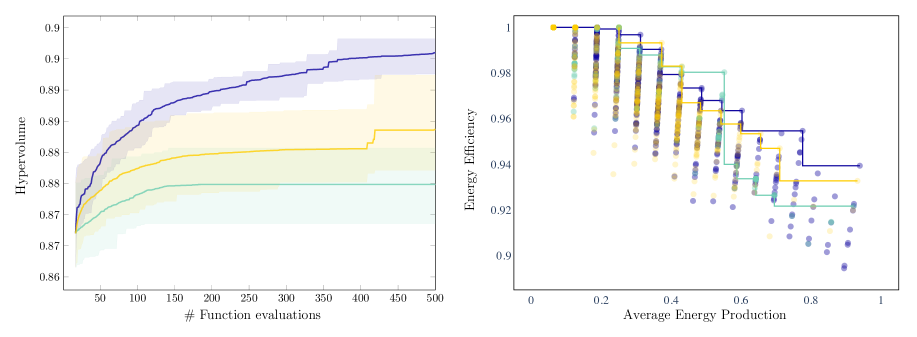
Figure 6: Compares windpark layout optimization results of NSGA-II (green), ENTMOOT (purple) and feasible sampling strategy (yellow). (left) Hypervolume bounded by Pareto frontier approximation after a certain number of function evaluations. (right) Best Pareto frontier approximation found for different algorithms based on hypervolume. Objectives are dimensionless due normalization based on physical limits.

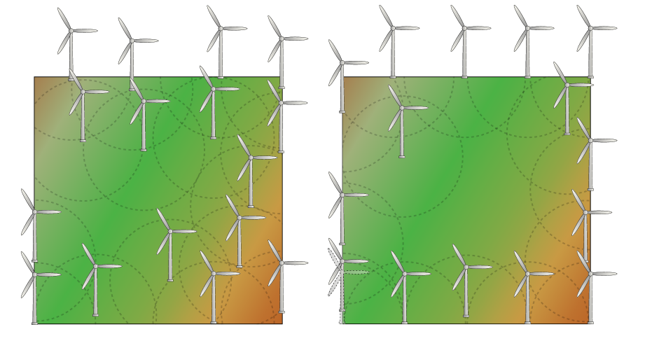
Figure 7: Example windpark layouts for highest average energy objective solutions not including initial samples, i.e. (left) ENTMOOT and (right) NSGA-II. Circles around wind turbines indicate the Equ. (28b) minimum distance constraints of 975 m between individual wind turbines. ENTMOOT is able to place all 16 turbines while NSGA-II is only able to place 15 due to constraint violation.

Fig. 6 shows the bounded hypervolume for different algorithms for a total of 500 black-box evaluations. For better comparison we include test runs for the initial sampling strategy where 500 total samples are generated. NSGA-II finds significantly better results early on when compared to a similar study presented in [RBB16], which is likely due to variety of initial feasible points provided, since GAs generate new black-box input proposals based on the previously observed population. However, even the feasible sampling strategy quickly outperforms NSGA-II, emphasizing the importance of providing feasible black-box input proposals. This is even more evident for solutions with large average energy production and low energy efficiency since these refer to windfarm layouts with a high number of wind turbines where more energy is produced with low energy efficiency due to wake effects. From an optimization perspective such solutions are more difficult due to Equ. (28b) minimum distance constraints enforced between all turbines that become increasingly restrictive for a growing number of wind turbines. Fig. 7 depicts layout proposals given by ENTMOOT and NSGA-II for highest average energy production, i.e. solutions with high number of turbines, when excluding the set of initial samples. While NSGA-II fails to place all 16 turbines due to constraint violation, ENTMOOT manages to find a feasible solution for all turbines available highlighting its capability to explore the entire Pareto frontier of non-dominated objective trade-offs. Moreover, ENTMOOT profits from its capability to explicitly handle input constraints. The presented 32-dimensional case study has a smaller effective dimensionality since only positions of active turbines influence the black-box outcome, e.g. if only one turbine is active, the problem becomes three dimensional. Since ENTMOOT can capture this hierarchical structure, it never revisits equivalent solutions and better uses the sampling budget. Fig. 6 depicts the best Pareto frontier approximations found by each algorithm and shows ENTMOOT’s outstanding performance compared to NSGA-II for high average energy production solutions due to guaranteed feasible input proposals even for highly-constrained problems. ENTMOOT also outperforms the feasible sampling strategy, highlighting the significance of using tree ensembles as surrogate models to learn multi-objective systems. Note that [RBB16] only tested on a discrete grid with varying resolution because continuous coordinates were deemed too difficult. With 500 iterations, ENTMOOT for the continuous case outperforms all methods presented in [RBB16] for the highest discretization resolution even after up to $10^{6}$ iterations. While one can argue that the windfarm layout benchmark presented here is cheap to evaluate, real-world layout planning will require many expensive dynamic fluid simulations, and sampling-efficient algorithms can help with quickly finding good solutions

4.4 Battery Material Optimization

$p$	parameter set picked for default values
$\epsilon_{\text{poros}}^{+}$	porosity of positive battery side
$\epsilon_{\text{active}}^{+}$	active material volume fraction of positive battery side
$R_{\text{particle}}^{+}$	particle radius of positive battery side
$C$	current that discharges the battery in one hour
$\lambda^{+}$	electrode thickness scaling factor of positive battery side
$\epsilon_{\text{poros}}^{-}$	porosity of negative battery side
$\epsilon_{\text{active}}^{-}$	active material volume fraction of negative battery side
$R_{\text{particle}}^{-}$	particle radius of negative battery side
$\lambda^{-}$	electrode thickness scaling factor of negative battery side
$I$	discharge current
$V$	discharge voltage
$t$	discharge time

Table 5: Battery benchmark table of notation.

4.5 General Model Description

Battery technology is a popular field of research and there are many examples in literature that successfully model key performance metrics, e.g. capacity degradation [Sev+19], by using data-driven approaches. In this section we consider Lithium-ion battery optimization: namely how to simultaneously achieve high energy and power density. For this exercise the open-source software PyBaMM [Sul+21] is used, which comprises a number of mathematical models for simulating the important physical processes that occur within batteries. PyBaMM makes extensive use of the CasADi framework [And+19] to solve the system of DAEs and the NumPy [Har+20] python package for array manipulation. Within the PyBaMM framework, the Single Particle Model with electrolyte effects (SPMe) [Mar+19] is chosen as it offers a good compromise between computational cost and accuracy (including electrolyte losses and particle diffusion). While recent works [Tra+20] and [Tim+21] have studied battery-state heterogeneity, we select a one-dimensional, isothermal formulation here for simplicity, noting that the proposed framework is agnostic to the form of the black-box model. The full suite of battery models available in PyBaMM is described in [Mar+20].

A typical Lithium-ion battery comprises layers of electrodes containing active material that host the ions at different open-circuit potentials. These electrodes are separated by non-conductive, electrolyte filled polymers, with layers alternating between anode (negative) and cathode (positive). The electrodes are usually coated onto both sides of metallic foils that form the current collectors, which are typically copper and aluminium. The battery charges and discharges when an external current is passed between the cell terminals, and ions flow internally within the electrolyte between the electrodes, completing redox reactions at the active-material surfaces. Each electrode is formed of a solid matrix mixture of active material, to support the intercalation of lithium ions, and carbon binder which structurally supports the active material and conducts electrons towards the reaction sites. The matrix is porous, allowing electrolyte to penetrate the material and conduct ions in the liquid phase to participate in the reactions. The active material in the anode is typically graphite and has an open-circuit potential close to zero, compared with lithium, and the active material in the cathode is commonly a transition metal or combination thereof, for example Nickel, Manganese and Cobalt or (NMC). The composition/chemistry of both electrodes, but especially the cathode, can vary quite significantly for different applications. Some materials, e.g., lithium-iron-phosphate (LFP), are more stable and longer lasting, but have a lower open-circuit voltage, and therefore, the resulting battery has lower power density.

Aside from chemistry, the dimensions of the layers and microstructural design of the materials also greatly affects whether a cell performs better as a high-energy or high-power cell. The losses within the cells are characterised by overpotentials that manifest by reducing the cell voltage, and these are typically dependent on the operating current. As batteries are usually operated within determined voltage windows for safety and longevity, the recoverable capacity (and cell voltage) decreases when cycling at higher rates. Two important transport related phenomena within the cell in particular are: ion migration within the electrolyte, and diffusion within the active material. The interlayer transport is largely determined by the volume fractions of the electrode constituents, which also in turn affect the tortuosity of the transport pathways. The porosity of the solid electrode matrix refers to the volume fraction of the space that is filled with electrolyte. A decreased porosity here results in a corresponding increase in active material volume (and therefore specific capacity); however, the transport is then on average more difficult, and the cell will not be able to operate at high power. Similarly, if the electrodes are made thicker then the overall active material volume fraction will increase compared to inactive components such as current collectors and separators, but transport losses will increase as ions have further to travel to reach all parts of the cell. Finally, another key microstructural parameter is the average size of active particles. Smaller particles will have better solid diffusion losses and a greater active surface area per volume, but may necessitate a greater binder volume fraction in order to keep them structurally stable and provide enough electron pathways to the increased number of active sites.

Given all the above considerations, this case study seeks to select a set of hyper-parameters using published parameter sets from the battery literature [Ai+19, Che+20, Eck+15, Eck+15a, Mar+19, Yan+17] and then explore various geometrical parameters in order to find an optimal high energy and high power combination. Table 5 lists the notation for this case study. The mean power and discharged energy of the battery cell form the objective functions, i.e. $f_{1}$ and $f_{2}$, respectively, and are defined as:

$$\begin{cases}f_{1}(\bm{x})=\overline{IV},\\ f_{2}(\bm{x})=\int_{0}^{t}IV\,dt,\end{cases}$$ (31)

where $I$ is the current, $V$ is the voltage and $t$ is discharge time. As simulations are performed on a 1-D domain an arbitrary cross-sectional area is assigned to the battery and determines the cell volume along with the layer thickness which is varied between cases. Cell volume is used to normalize the objective functions making them comparable for different runs.

4.5.1 Optimization Benchmark

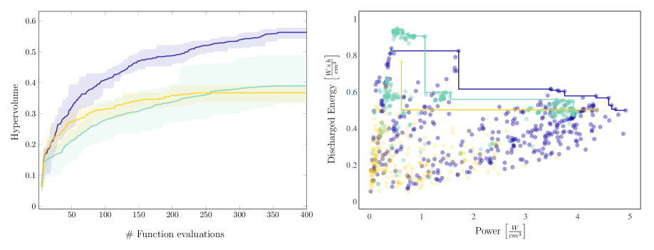
Figure 8: Compares battery optimization results of NSGA-II (green), ENTMOOT (purple) and feasible sampling strategy (yellow). (left) Hypervolume bounded by Pareto frontier approximation after a certain number of function evaluations. (right) Best Pareto frontier approximation found for different algorithms based on hypervolume.

Reasonable bounds for all optimization variables are given in Equ. (32h) - Equ. (32q), with variable $p$ indicating the parameter set selected. We model the variable $p$ as a categorical variable, as it is difficult to quantify a distance between different parameter sets $\{\text{Ai2019},\ \text{Chen2020},\ \text{Ecker2015},\ \text{Marquis2019},\ \text{Yang2017}\}$. Variables $\epsilon_{\text{poros}}$, $\epsilon_{\text{active}}$ and $R_{\text{particle}}$ denote porosity, active material volume fraction and particle radius and are optimized for both positive and negative side of the battery, i.e. indicated by $+$ and $-$. The negative and positive side electrode thickness is scaled by optimization variable $\lambda$ allowing a continuous range between half and double the size of the default electrode. Since porosity translates to the volume fraction of the electrolyte, Equ. (32a) and Equ. (32b) limit the sum of porosity and active material volume fraction $\epsilon_{\text{active}}$ to $0.95$ leaving a volume fraction of $5\%$ for binder material. Different battery specifications are designed for certain C-rate ranges, i.e. $1\text{C}$ translates to the current that discharges the battery in 1 hour, and is denoted by variable $C$. Too high values of $C$ certain battery designs cause PyBaMM simulations to fail. To reduce the number of failed simulations we introduce custom upper bounds for $C$ in Equ. (32c) - Equ.(32g) based on preliminary studies for all parameter sets in $p\in\{\text{Ai2019},\ \text{Chen2020},\ \text{Ecker2015},\ \text{Marquis2019},\ \text{Yang2017}\}$ without modifying other optimization variables. Both objectives, i.e.  power and discharged energy, are normalized based on best minimum and maximum values observed throughout all computational runs. In summary, this case study has one categorical variable describing the underlying parameter set that is being used, i.e. Equ. (32h), and nine continuous variables denoting various design parameters of the battery cell that can be optimized, i.e. Equ. (32i) - Equ. (32q). Equ. (32a) - Equ. (32g) comprise seven additional constraints for input variables.

Required Constraints

$$\epsilon_{\text{poros}}^{-}+\epsilon_{\text{active}}^{-}\leq 0.95$$ (32a)

$$\epsilon_{\text{poros}}^{+}+\epsilon_{\text{active}}^{+}\leq 0.95$$ (32b)

$$(p=\text{Ai2019})\rightarrow C\leq 3.2$$ (32c)

$$(p=\text{Chen2020})\rightarrow C\leq 2.2$$ (32d)

$$(p=\text{Ecker2015})\rightarrow C\leq 8.2$$ (32e)

$$(p=\text{Marquis2019})\rightarrow C\leq 5.2$$ (32f)

$$(p=\text{Yang2017})\rightarrow C\leq 8.2$$ (32g)

$$p\in\{\text{Ai2019},\ \text{Chen2020},\ \text{Ecker2015},\ \text{Marquis2019},\ \text{Yang2017}\}$$ (32h)

$$C\in\left[0.5,8.2\right]$$ (32i)

$$\epsilon_{\text{poros}}^{-}\in\left[0.2,0.7\right]$$ (32j)

$$\epsilon_{\text{active}}^{-}\in\left[0.2,0.7\right]$$ (32k)

$$R_{\text{particle}}^{-}\in\left[$1\text{\times}{10}^{-6}$,$20\text{\times}{10}^{-6}$[m]\right]$$ (32l)

$$\epsilon_{\text{poros}}^{+}\in\left[0.2,0.7\right]$$ (32m)

$$\epsilon_{\text{active}}^{+}\in\left[0.2,0.7\right]$$ (32n)

$$R_{\text{particle}}^{+}\in\left[$1\text{\times}{10}^{-6}$,$20\text{\times}{10}^{-6}$[m]\right]$$ (32o)

$$\lambda^{-}\in\left[0.5,2.0\right]$$ (32p)

$$\lambda^{+}\in\left[0.5,2.0\right]$$ (32q)

A procedure similar to Algorithm 1 provides ten feasible initial points to all competing methods. We fix the categorical variable $p\in\{\text{Ai2019},\ \text{Chen2020},\ \text{Ecker2015},\ \text{Marquis2019},\ \text{Yang2017}\}$ for individual points to obtain two points for each possible parameter set $p$. For the general case, the method extends Equ. (30) with similarity measures, e.g. Equ. (10) and Equ. (12), to increase diversity in initial samples with respect to categorical features.
Fig. 8 shows hypervolume improvement and best Pareto frontier approximations for the battery design benchmark. All methods are capable improving the hypervolume of the objective space. Compared to the Section 4.3 benchmark the constraints given in Equ. (32) are less restrictive making feasible solutions more attainable and allowing NSGA-II to surpass the feasible sampling strategy. ENTMOOT manages to outperform other strategies for all different random seeds considered. The Fig. 8 best Pareto frontier approximations derived by competing methods show that NSGA-II spends a large amount of evaluation budget to improve already explored points while ENTMOOT is actively exploring the entire objective space. ENTMOOT especially dominates when it comes to high power solutions which are dominated by high C-rates. Since, ENTMOOT guarantees feasibility of proposed solutions, C-rates are kept below the bounds specified in Equ. (32c) - Equ.(32g) allowing for a higher frequency of successful simulations. The feasible sampling strategy manages to only find two non-dominated points for the Pareto frontier approximation.

5 Conclusion

Energy systems with multiple opposing objects are challenging to optimize due to complex system behavior, highly restrictive input constraints and large feature spaces with heterogenous variable types. The resulting problems are often handled using multi-objective Bayesian optimization, owing to relatively high sampling efficiency and ability to directly include input constraints. Tree-based models represent promising candidates for this class of optimization problems, as they are well-suited for nonlinear/discontinuous functions and naturally support discrete/categorical features. Nevertheless, uncertainty quantification and optimization over tree models are non-trivial, limiting their deployment in black-box optimization.

Given the above, this work introduces a multi-objective black-box optimization framework based on the tree-based ENTMOOT tool. The proposed all-in-one strategy addresses all of the above challenges, while also providing better sampling efficiency compared to the popular state-of-the-art tool NGSA-II. In a comprehensive numerical study, we demonstrate the advantages of the proposed framework on both synthetic problems and energy-related benchmarks, including windfarm layout optimization and lithium-ion battery design with two objective functions. In both energy-related benchmarks, ENTMOOT identifies better Pareto frontiers, and in significantly fewer iterations, compared to NGSA-II and a random search strategy. Due to its versatility and sampling efficiency we envision ENTMOOT to be strongly relevant to real-world and industrial settings where experimental black-box evaluations are expensive. While the numerical studies only consider bi-objective problems, the proposed method also applies to case studies with more than two objective functions. Future research will focus on other applications with more objective functions that can benefit from the proposed method.

6 Acknowledgments

This work was supported by BASF SE, Ludwigshafen am Rhein, EPSRC Research Fellowships to RM (EP/P016871/1) and CT (EP/T001577/1), and an Imperial College Research Fellowship to CT. TT acknowledges funding from the EPSRC Faraday Institution Multiscale Modelling Project (EP/S003053/1, FIRG003)

References

- [Ai+19] Weilong Ai, Billy Wu, Johannes Sturm and Andreas Jossen “Electrochemical Thermal-Mechanical Modelling of Stress Inhomogeneity in Lithium-Ion Pouch Cells Electrochemical Thermal-Mechanical Modelling of Stress Inhomogeneity in Lithium-Ion Pouch Cells” In Journal of the Electrochemical Society 167.1, 2019, pp. 013512 DOI: 10.1149/2.0122001JES
- [And+19] Joel A.E. Andersson, Joris Gillis, Greg Horn, James B. Rawlings and Moritz Diehl “CasADi: a software framework for nonlinear optimization and optimal control” In Mathematical Programming Computation 11.1, 2019, pp. 1–36 DOI: 10.1007/s12532-018-0139-4
- [BCF09] E. Brochu, M. Cora and N. Freitas “A Tutorial on Bayesian Optimization of Expensive Cost Functions, with Application to Active User Modeling and Hierarchical Reinforcement Learning” In ArXiv 1012.2599, 2009
- [BCK08] S. Boriah, V. Chandola and V. Kumar “Similarity Measures for Categorical Data: A Comparative Evaluation” In Proceedings of the SIAM International Conference on Data Mining 30, 2008, pp. 243–254
- [BD20] J. Blank and K. Deb “Pymoo: Multi-Objective Optimization in Python” In IEEE Access 8, 2020, pp. 89497–89509
- [Bey+18] Burcu Beykal, Fani Boukouvala, Christodoulos A Floudas and Efstratios N Pistikopoulos “Optimal design of energy systems using constrained grey-box multi-objective optimization” In Computers & Chemical Engineering 116 Elsevier, 2018, pp. 488–502
- [BI18] A. Bhosekar and M. Ierapetritou “Advances in surrogate based modeling, feasibility analysis, and optimization: A review” In Computers & Chemical Engineering 108, 2018, pp. 250–267
- [BMF16] Fani Boukouvala, Ruth Misener and Christodoulos A. Floudas “Global optimization advances in Mixed-Integer Nonlinear Programming, MINLP, and Constrained Derivative-Free Optimization, CDFO” In European Journal of Operational Research 252.3, 2016, pp. 701–727
- [Bre01] Leo Breiman “Random Forests” In Machine learning 45.1 Springer, 2001, pp. 5–32
- [BSL18] Eric Bradford, Artur M Schweidtmann and Alexei Lapkin “Efficient multiobjective optimization employing Gaussian processes, spectral sampling and a genetic algorithm” In Journal of Global Optimization 71.2 Springer, 2018, pp. 407–438
- [BY03] Peter Bühlmann and Bin Yu “Boosting with the L2 loss: regression and classification” In Journal of the American Statistical Association 98.462 Taylor & Francis, 2003, pp. 324–339
- [Che+20] Chang-Hui Chen, Ferran Brosa Planella, Kieran O’Regan, Dominika Gastol, W. Widanage and Emma Kendrick “Development of Experimental Techniques for Parameterization of Multi-scale Lithium-ion Battery Models” In Journal of The Electrochemical Society 167.8, 2020, pp. 080534 DOI: 10.1149/1945-7111/ab9050
- [CJ97] Dennis D. Cox and Susan John “SDO: A Statistical Method for Global Optimization” In Multidisciplinary Design Optimization: State of the Art Society for Industrial & Applied Mathematics, 1997, pp. 315–329
- [CLV+07] Carlos A Coello Coello, Gary B Lamont and David A Van Veldhuizen “Evolutionary algorithms for solving multi-objective problems” Springer, 2007
- [Deb+02] Kalyanmoy Deb, Amrit Pratap, Sameer Agarwal and TAMT Meyarivan “A fast and elitist multiobjective genetic algorithm: NSGA-II” In IEEE Transactions on Evolutionary Computation 6.2 IEEE, 2002, pp. 182–197
- [Del+16] N Delgarm, B Sajadi, F Kowsary and S Delgarm “Multi-objective optimization of the building energy performance: A simulation-based approach by means of particle swarm optimization (PSO)” In Applied Energy 170 Elsevier, 2016, pp. 293–303
- [Eck+15] Madeleine Ecker, Thi Kim, Dung Tran, Philipp Dechent and Stefan Käbitz “Parameterisation of a Physico-Chemical Model of a Lithium-Ion Battery Part I : Determination of Parameters” In Journal of The Electrochemical Society 162.9, 2015, pp. A1836–A1848
- [Eck+15a] Madeleine Ecker, Stefan Käbitz, Izaro Laresgoiti and Dirk Uwe Sauer “Parameterization of a Physico-Chemical Model of a Lithium-Ion Battery: II. Model Validation” In Journal of The Electrochemical Society 162.9, 2015, pp. A1849–A1857 DOI: 10.1149/2.0541509jes
- [FF95] Carlos M Fonseca and Peter J Fleming “An overview of evolutionary algorithms in multiobjective optimization” In Evolutionary Computation 3.1 MIT Press, 1995, pp. 1–16
- [Fis58] Walter D Fisher “On grouping for maximum homogeneity” In Journal of the American statistical Association 53.284 Taylor & Francis, 1958, pp. 789–798
- [Fra18] Peter I. Frazier “A Tutorial on Bayesian Optimization” In ArXiv 1807.02811, 2018
- [Fri00] Jerome H. Friedman “Greedy Function Approximation: A Gradient Boosting Machine” In Annals of Statistics 29, 2000, pp. 1189–1232
- [Fri02] Jerome H Friedman “Stochastic gradient boosting” In Computational Statistics & Data Analysis 38.4, 2002, pp. 367–378
- [FSK08] A. Forrester, A. Sóbester and A. Keane “Engineering Design via Surrogate Modelling: A Practical Guide” Wiley, 2008
- [FW16] P.. Frazier and J. Wang “Bayesian optimization for materials design” In Information Science for Materials Discovery and Design Springer, 2016, pp. 45–75
- [GP02] A. Giloni and M. Padberg “Alternative Methods of Linear Regression” In Mathematical and Computer Modeling 35, 2002, pp. 361–374
- [Har+07] Ken Harada, Jun Sakuma, Isao Ono and Shigenobu Kobayashi “Constraint-handling method for multi-objective function optimization: Pareto descent repair operator” In International Conference on Evolutionary Multi-Criterion Optimization, 2007, pp. 156–170 Springer
- [Har+20] Charles R. Harris et al. “Array Programming with NumPy” In Nature 585.February, 2020, pp. 357–362 DOI: 10.1038/s41586-020-2649-2
- [HF17] Zahra Hajabdollahi and Pei-Fang Fu “Multi-objective based configuration optimization of SOFC-GT cogeneration plant” In Applied Thermal Engineering 112 Elsevier, 2017, pp. 549–559
- [HHL11] Frank Hutter, Holger H. Hoos and Kevin Leyton-Brown “Sequential Model-Based Optimization for General Algorithm Configuration” In Proceedings of the 5th International Conference on Learning and Intelligent Optimization, LION’05 Rome, Italy: Springer-Verlag, 2011, pp. 507–523
- [HM12] C-L Hwang and Abu Syed Md Masud “Multiple objective decision making—methods and applications: a state-of-the-art survey” Springer Science & Business Media, 2012
- [HN17] Hossein Haddadian and Reza Noroozian “Multi-microgrids approach for design and operation of future distribution networks based on novel technical indices” In Applied energy 185 Elsevier, 2017, pp. 650–663
- [Hu+16] Yuan Hu, Zhaohong Bie, Tao Ding and Yanling Lin “An NSGA-II based multi-objective optimization for combined gas and electricity network expansion planning” In Applied energy 167 Elsevier, 2016, pp. 280–293
- [Jav+20] Mohammad Javadi et al. “A multi-objective model for home energy management system self-scheduling using the epsilon-constraint method” In 2020 IEEE 14th International Conference on Compatibility, Power Electronics and Power Engineering (CPE-POWERENG) 1, 2020, pp. 175–180 IEEE
- [KBB18] Morgan T Kelley, Ross Baldick and Michael Baldea “Demand response operation of electricity-intensive chemical processes for reduced greenhouse gas emissions: application to an air separation unit” In ACS Sustainable Chemistry & Engineering 7.2 ACS Publications, 2018, pp. 1909–1922
- [Ke+17] Guolin Ke et al. “LightGBM: A Highly Efficient Gradient Boosting Decision Tree” In Proceedings of the 31st International Conference on Neural Information Processing Systems, NIPS’17 Long Beach, California, USA: Curran Associates Inc., 2017, pp. 3149–3157
- [KH01] Roger Koenker and Kevin F. Hallock “Quantile Regression” In Journal of Economic Perspectives 15.4, 2001, pp. 143–156
- [KHJ86] I Katic, Jørgen Højstrup and Niels Otto Jensen “A simple model for cluster efficiency” In European Wind Energy Association Conference and Exhibition 1, 1986, pp. 407–410
- [Kno06] Joshua Knowles “ParEGO: A hybrid algorithm with on-line landscape approximation for expensive multiobjective optimization problems” In IEEE Transactions on Evolutionary Computation 10.1 IEEE, 2006, pp. 50–66
- [Kum+10] Manoj Kumar, Mohammad Husain, Naveen Upreti and Deepti Gupta “Genetic algorithm: Review and application” In Available at SSRN 3529843, 2010
- [Kur90] Frank Kursawe “A variant of evolution strategies for vector optimization” In International Conference on Parallel Problem Solving from Nature, 1990, pp. 193–197 Springer
- [LL17] Changhong Liu and Lin Liu “Optimizing battery design for fast charge through a genetic algorithm based multi-objective optimization framework” In ECS Transactions 77.11 IOP Publishing, 2017, pp. 257
- [Mar+19] Scott G. Marquis, Valentin Sulzer, Robert Timms, Colin P. Please and S. Chapman “An asymptotic derivation of a single particle model with electrolyte” In Journal of The Electrochemical Society 166.15, 2019, pp. A3693–A3706 DOI: 10.1149/2.0341915jes
- [Mar+20] Scott Marquis, Robert Timms, Valentin Sulzer, Colin P Please and S Jon Chapman “A Suite of Reduced-Order Models of a Single-Layer Lithium-Ion Pouch Cell” In Journal of the Electrochemical Society 167.14 IOP Publishing, 2020, pp. 140513 DOI: 10.1149/1945-7111/abbce4
- [MCB21] Jamie A Manson, Thomas W Chamberlain and Richard A Bourne “MVMOO: Mixed variable multi-objective optimisation” In Journal of Global Optimization Springer, 2021, pp. 1–22
- [Mei06] Nicolai Meinshausen “Quantile Regression Forests” In Journal of Machine Learning Research 7, 2006, pp. 983–999
- [Mes+00] Achille Messac, Glynn J Sundararaj, Ravindra V Tappeta and John E Renaud “Ability of objective functions to generate points on nonconvex Pareto frontiers” In AIAA Journal 38.6, 2000, pp. 1084–1091
- [Mis+20] Miten Mistry, Dimitrios Letsios, Gerhard Krennrich, Robert M Lee and Ruth Misener “Mixed-Integer Convex Nonlinear Optimization with Gradient-Boosted Trees Embedded” In INFORMS Journal on Computing, 2020 DOI: 10.1287/ijoc.2020.0993
- [Miš17] Velibor V Mišić “Optimization of Tree Ensembles” In ArXiv 1705.10883, 2017
- [Moč89] J. Močkus “Bayesian Approach to Global Optimization: Theory and Applications” Kluwer Academic Publishers, 1989
- [MSG20] Martin János Mayer, Artúr Szilágyi and Gyula Gróf “Environmental and economic multi-objective optimization of a household level hybrid renewable energy system by genetic algorithm” In Applied Energy 269 Elsevier, 2020, pp. 115058
- [NFP11] D.. Negoescu, P.. Frazier and W.B. Powell “The knowledge gradient algorithm for sequencing experiments in drug discovery” In INFORMS Journal on Computing 1.23, 2011, pp. 46–363
- [Olo+18] Simon Olofsson, Mohammad Mehrian, Roberto Calandra, Liesbet Geris, Marc Peter Deisenroth and Ruth Misener “Bayesian multiobjective optimisation with mixed analytical and black-box functions: Application to tissue engineering” In IEEE Transactions on Biomedical Engineering 66.3 IEEE, 2018, pp. 727–739
- [Par19] Vilfredo Pareto “Manuale di economia politica: con una introduzione alla scienza sociale” Società editrice libraria, 1919
- [Pis+21] E N Pistikopoulos et al. “Process systems engineering – The generation next?” In Computers & Chemical Engineering 147, 2021, pp. 107252
- [RBB16] S Rodrigues, Pavol Bauer and Peter AN Bosman “Multi-objective optimization of wind farm layouts–Complexity, constraint handling and scalability” In Renewable and Sustainable Energy Reviews 65 Elsevier, 2016, pp. 587–609
- [RW06] C.. Rasmussen and C… Williams “Gaussian Processes for Machine Learning” The MIT Press, 2006
- [RY03] Thomas Runarsson and Xin Yao “Constrained evolutionary optimization” In Evolutionary Optimization Springer, 2003, pp. 87–113
- [SC04] Margarita R Sierra and Carlos A Coello Coello “A new multi-objective particle swarm optimizer with improved selection and diversity mechanisms” In Technical Report of CINVESTAV-IPN, 2004
- [Sch85] J David Schaffer “Some experiments in machine learning using vector evaluated genetic algorithms”, 1985
- [Sev+19] Kristen A Severson et al. “Data-driven prediction of battery cycle life before capacity degradation” In Nature Energy 4.5 Nature Publishing Group, 2019, pp. 383–391
- [SH10] Sepehr Sanaye and Hassan Hajabdollahi “Thermal-economic multi-objective optimization of plate fin heat exchanger using genetic algorithm” In Applied Energy 87.6 Elsevier, 2010, pp. 1893–1902
- [Sha+16] Bobak Shahriari, Kevin Swersky, Ziyu Wang, Ryan P Adams and Nando Freitas “Taking the Human Out of the Loop: A Review of Bayesian Optimization” In Proceedings of the IEEE 104.1, 2016, pp. 148–175
- [Sno+15] J. Snoek et al. “Scalable Bayesian Optimization Using Deep Neural Networks” In Proceedings of the 32nd International Conference on International Conference on Machine Learning 37, 2015, pp. 2171–2180
- [Sul+21] Valentin Sulzer, Scott Marquis, Robert Timms, Martin Robinson and S. Chapman “Python Battery Mathematical Modelling (PyBaMM)” In Journal of Open Research Software 9.1, 2021 DOI: doi.org/10.5334/ jors.309
- [The+21] Alexander Thebelt, Jan Kronqvist, Miten Mistry, Robert M Lee, Nathan Sudermann-Merx and Ruth Misener “ENTMOOT: A framework for optimization over ensemble tree models” In Computers & Chemical Engineering 151 Elsevier, 2021, pp. 107343
- [The18] The scikit-optimize contributors “scikit-optimize/scikit-optimize: v0.5.2” Zenodo, 2018 URL: https://doi.org/10.5281/zenodo.1207017
- [Tim+21] Robert Timms, Scott G. Marquis, Valentin Sulzer, Colin P. Please and S. Chapman “Asymptotic reduction of a lithium-ion pouch cell model” In SIAM Journal on Applied Mathematics 81.3, 2021, pp. 765–788 DOI: 10.1137/20M1336898
- [Tom88] J.. Tomlin “Special ordered sets and an application to gas supply operations planning” In Mathematical Programming 42.1, 1988, pp. 69–84
- [Tra+20] T.. Tranter et al. “Probing Heterogeneity in Li-Ion Batteries with Coupled Multiscale Models of Electrochemistry and Thermal Transport using Tomographic Domains” In Journal of The Electrochemical Society 167, 2020, pp. 110538 DOI: 10.1149/1945-7111/aba44b
- [Van99] David Allen Van Veldhuizen “Multiobjective evolutionary algorithms: classifications, analyses, and new innovations” Air Force Institute of Technology, 1999
- [VTD15] Pedro P Vergara, Ricardo Torquato and Luiz CP Da Silva “Towards a real-time Energy Management System for a Microgrid using a multi-objective genetic algorithm” In 2015 IEEE Power & Energy Society General Meeting, 2015, pp. 1–5 IEEE
- [WHE14] Stefan Wager, Trevor Hastie and Bradley Efron “Confidence Intervals for Random Forests: The Jackknife and the Infinitesimal Jackknife” In Journal of Machine Learning Research 15, 2014, pp. 1625–1651
- [Yan+17] Xiao Guang Yang, Yongjun Leng, Guangsheng Zhang, Shanhai Ge and Chao Yang Wang “Modeling of lithium plating induced aging of lithium-ion batteries: Transition from linear to nonlinear aging” In Journal of Power Sources 360 Elsevier, 2017, pp. 28–40 DOI: 10.1016/j.jpowsour.2017.05.110
- [Yin+14] Wing Yin Kwong, Peter Yun Zhang, David Romero, Joaquin Moran, Michael Morgenroth and Cristina Amon “Multi-objective wind farm layout optimization considering energy generation and noise propagation with NSGA-II” In Journal of Mechanical Design 136.9 American Society of Mechanical Engineers, 2014, pp. 091010
- [Yu+15] Wei Yu, Baizhan Li, Hongyuan Jia, Ming Zhang and Di Wang “Application of multi-objective genetic algorithm to optimize energy efficiency and thermal comfort in building design” In Energy and Buildings 88 Elsevier, 2015, pp. 135–143
- [Zad63] Lofti Zadeh “Optimality and non-scalar-valued performance criteria” In IEEE Transactions on Automatic Control 8.1 IEEE, 1963, pp. 59–60
- [Zho+16] Nan Zhou, Nian Liu, Jianhua Zhang and Jinyong Lei “Multi-objective optimal sizing for battery storage of PV-based microgrid with demand response” In Energies 9.8 MDPI, 2016, pp. 591