Episodic deluges in simulated hothouse climates

Earth’s distant past and potentially its future include extremely warm “hothouse”¹ climate states, but little is known about how the atmosphere behaves in such states. One distinguishing characteristic of hothouse climates is that they feature lower-tropospheric radiative heating, rather than cooling, due to the closing of the water vapor infrared window regions². Previous work has suggested that this could lead to temperature inversions and significant changes in cloud cover³, ⁴, ⁵, ⁶, but no previous modeling of the hothouse regime has resolved convective-scale turbulent air motions and cloud cover directly, thus leaving many questions about hothouse radiative heating unanswered. Here, we conduct simulations that explicitly resolve convection and find that lower-tropospheric radiative heating in hothouse climates causes the hydrologic cycle to shift from a quasi-steady regime to a “relaxation oscillator” regime, in which precipitation occurs in short and intense outbursts separated by multi-day dry spells. The transition to the oscillatory regime is accompanied by strongly enhanced local precipitation fluxes, a significant increase in cloud cover, and a transiently positive (unstable) climate feedback parameter. Our results indicate that hothouse climates may feature a novel form of “temporal” convective self-organization, with implications for both cloud coverage and erosion processes.

For the past few million years, Earth’s climate has been characterized by fairly cool conditions, with repeated transitions between glacial and interglacial climates⁷. On longer timescales, however, the range of Earth’s climate states is far wider. In the Hadean and Archean⁸, ⁹, as well as in the aftermath of Neoproterozoic Snowball events¹⁰, high carbon dioxide levels may have elevated surface temperatures by tens of degrees Kelvin compared to today. In the distant future, increases in solar luminosity will cause surface temperature to increase and eventually drive Earth through a runaway greenhouse transition¹¹. No matter the forcing mechanism, warming of Earth’s climate causes atmospheric water vapor to accumulate rapidly, strengthening the water vapor greenhouse effect by rendering more of the infrared spectrum opaque. With sufficient warming, even the most weakly absorbing spectral “window” regions in the thermal infrared are closed off and the lower troposphere can no longer cool by emitting infrared radiation to space¹², ¹³. However, because water vapor also absorbs in the near-infrared ², tropospheric absorption of incoming solar radiation persists in extremely warm climates, eventually yielding net lower-tropospheric radiative heating (LTRH). This phenomenon may also occur on the intensely-irradiated day sides of tidally-locked exoplanets⁴, the climates of which are strongly influenced by convection near the substellar point ¹⁴, ¹⁵, ¹⁶.

Simulations of hothouse climates

We investigated hothouse climates using a convection-resolving model in which radiative and convective heating rates are constrained to be in time-mean balance ¹⁷. The model we employ (DAM¹⁸) is fully compressible and nonhydrostatic, and is well suited to simulating very warm climates in two key respects: 1) it takes into account the full thermodynamics of moist air, including changes in atmospheric pressure due to condensation and the effect of water on the heat capacity of air; and 2) the radiative transfer scheme has been modified to remain accurate in very warm climates¹⁷. For simulations with a time-evolving sea surface temperature (SST), the model SST is evolved according to the sum of surface enthalpy fluxes, radiative fluxes, and a prescribed ocean heat sink; we also performed simulations with fixed SST. Our baseline simulations were conducted on a 72 km $\times$ 72 km square grid with doubly-periodic horizontal boundary conditions. Further information about our model setup is available in the Methods section¹⁷.

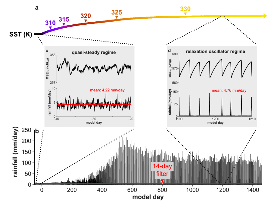
Figure 1: Transition to the relaxation oscillator regime due to increased insolation. Results are from a simulation initiated from an equilibrated state with a mean SST of 305 K but with a 10% increase in the solar constant, imposed on model day 0 in this figure. (a) 14-day-filtered SST with first-crossings indicated for 5-K increments above 305 K. (b) Hourly (black) and 14-day-filtered (red) precipitation. (c-d) Hourly precipitation and mean near-surface ($z<1$ km) moist static energy (MSE_ns) over 20-day intervals before and after the transition to the relaxation oscillator regime. Moist static energy is defined as $\mathrm{MSE}=c_{p}T+Lq_{v}+gz$, where $c_{p}$ (J/kg/K) is the heat capacity of air at constant pressure, $T$ (K) is the temperature, $L$ (J/kg) is the latent heat of vaporization, $q_{\mathrm{v}}$ (kg/kg) is the specific humidity, $g$ (m/s) is the gravitational acceleration, and $z$ (m) is the altitude.

Figure 1 shows results from a convection-resolving simulation that was initiated with an SST comparable to the warmest on Earth today (305 K, or 32 ^∘C), but with a 10% increase in the solar constant — equivalent to Earth about 1 billion years in the future, or on an orbit about 5% closer to the Sun today. In response to this large solar forcing, the model warms rapidly and reaches a new equilibrium at a mean SST of about 330 K (57 ^∘C) within four years of model-time. A fundamental shift in state is evident in Figures 1b–d, which show time series of hourly precipitation and near-surface moist static energy during the model evolution. The early stages of the simulation are in a quasi-steady convective regime, with hourly precipitation rates exhibiting noisy fluctuations about a mean of approximately 5 mm/day. Later in the simulation, as the SST warms above about 320 K, the nature of the precipitation changes fundamentally. Rather than exhibiting noisy fluctuations about the mean, precipitation occurs in large outbursts lasting a few hours, separated by regular multi-day dry spells during which there is essentially no precipitation. As in a canonical relaxation oscillator¹⁹, ²⁰, the latter regime is characterized by repeated sequences of slow destabilization and fast stabilization (Fig. 1d); hence we refer to this hothouse state as a “relaxation oscillator” or “oscillatory” regime. Since our simulations receive constant diurnally-averaged insolation¹⁷, the emergence of periodic behavior must be the result of radiative-convective feedbacks. Across the transition to the relaxation oscillator regime, the intensifying dry spells balance the increasingly large outbursts of precipitation such that time-mean rainfall before and after the transition changes by only about 10% (Figure 1b–d, 14-day-filtered rainfall), as predicted by mean energetic constraints²¹, ²². However, the maximum domain-mean hourly rain rates increase by an order of magnitude in the oscillatory regime.

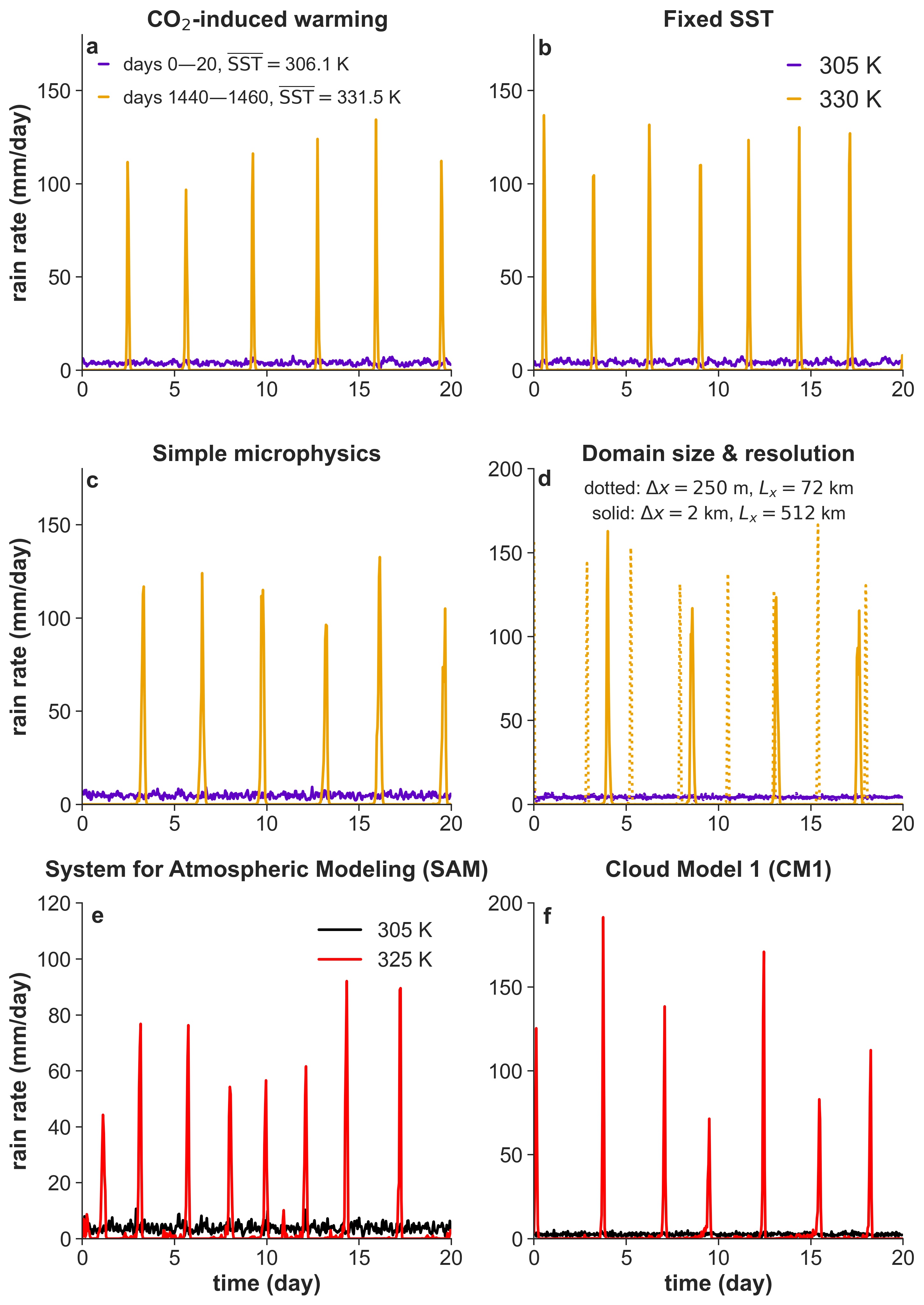
Figure E3: Tests of the robustness of the oscillatory transition. Domain-mean precipitation from two periods of (a) the FCO2 simulation with mean SSTs of 306.1 K and 331.5 K; (b) the fixedSST suite at 305 K and 330 K; (c) the fixedSST_sm suite, which use the simplified microphysics parameterization described in the Methods¹⁷; (d) fixed-SST simulations with finer horizontal resolution ($\Delta x=250$ m; fixedSST_hires) or on a larger domain ($L_{x}=512$ km; fixedSST_large). (e) The same quantity from simulations conducted with the System for Atmospheric Modeling (SAM)²¹ at fixed SSTs of 305 and 325 K. (f) As in (e), but for the Cloud Model 1 (CM1)²².

While Figure 1 shows that the oscillatory regime can result from solar-forced warming, the closing of the water vapor spectral windows is fundamentally tied to increased temperature and should occur regardless of the forcing mechanism. Indeed, our tests suggest that the oscillatory state is a general property of very warm and moist atmospheres simulated by convection-resolving models, being robust to forcing mechanism, microphysics scheme, domain size and resolution, and choice of convection-resolving model (Fig. E3). To further confirm the central importance of lower-tropospheric radiative heating, we conducted simulations across a range of surface temperatures with idealized time-invariant radiative heating profiles that resemble either cool-climate conditions (with radiative cooling throughout the troposphere) or hothouse conditions (with lower-tropospheric radiative heating). The cool-climate radiative heating profiles produce quasi-steady convective behavior at all temperatures (LTRH$\_$off; Fig. 2a,d), whereas the hothouse-type radiative heating profiles produce the relaxation oscillator regime at all temperatures (LTRH$\_$on; Fig. 2c,f). The simulations with radiation calculated interactively interpolate between these two regimes (Fig. 2b,e), suggesting that lower-tropospheric radiative heating is the key characteristic of hothouse climates that drives the transition to the relaxation oscillator regime.

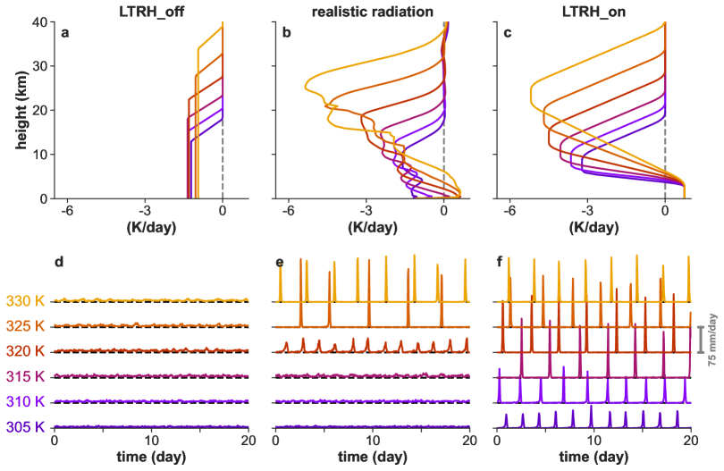
Figure 2: The oscillatory regime is induced by lower-tropospheric radiative heating. (Top row) Vertical profiles of radiative heating from the (a) LTRH_off, (b) fixedSST, and (c) LTRH_on simulations¹⁷. The fixedSST simulations use realistic radiative transfer calculated with the model-generated vertical profiles of temperature and absorber densities, while for the other two experiments, the radiative heating profiles are prescribed to resemble either cool-climate conditions (radiative cooling throughout the troposphere; LTRH_off) or hothouse conditions (radiative heating in the lower troposphere; LTRH_on). Cool to warm colors indicate increasing SST. (Bottom row, panels d–e) 20-day time series of domain-mean precipitation from the simulations. For visual clarity, the precipitation data is offset vertically by 75 mm/day (gray scale bar at right) for each 5-K increment of SST.

Physical basis of the oscillatory regime

To reveal the mechanism behind the oscillatory state, we studied high-frequency output from fixed-SST simulations at 330 K. This output shows that the oscillatory state consists of three main phases: recharge, triggering, and discharge (Fig. 3). An animation of model output in the oscillatory state can be viewed in the Supplementary Video, and a summary schematic of the phases of the oscillatory state is presented in Figure 4.

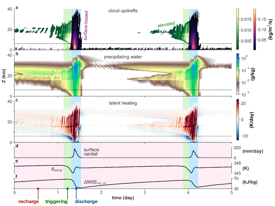
Figure 3: Mechanism of the oscillatory regime as revealed by high-frequency model output. (a–c) Time-vs-height plots of (a) cloud updraft mass flux, (b) precipitating water mass fraction $q_{p}$, and (c) latent heating from the fixedSST simulation at 330 K. Convective mass flux was divided into “surface-based” and “elevated” categories using a passive tracer¹⁷. (d–f) Timeseries of (d) domain-mean surface precipitation, (e) $\theta_{\mathrm{inhib}}$, the mean potential temperature in the inhibition layer ($2000<z<5500$ m), and (f) difference in mean moist static energy between the near-surface layer ($z<1$ km) and the upper troposphere ($25<z<35$ km) from the same simulation. The discharge phases in this figure (blue shading) are identified as intervals with a surface precipitation rate above 5 mm/day. The triggering phases (green shading) begin when the hourly-mean latent heating rate in the inhibition layer is more negative than -2 K/day and the surface precipitation rate is less than 1 mm/day, and end when the ensuing discharge period commences. The recharge phases occur between the end of a discharge phase and the beginning of a triggering phase. The dotted horizontal lines in panels a–c marks the level of zero radiative heating (i.e., the transition from time-mean radiative heating to cooling).

During an outburst of precipitation (discharge phase), the lower troposphere is flooded with negatively-buoyant downdrafts of cold and dry air with low moist static energy (Fig. 3f, Supplementary Video). Over the course of the ensuing recharge phase, LTRH keeps the surface and the upper troposphere decoupled by increasing the mean potential temperature in the intervening “inhibition layer” (Fig. 3e) and suppressing surface buoyancy fluxes. With the inhibition layer effectively throttling surface-based convection, surface evaporation humidifies the near-surface air without any compensating ventilation into the upper troposphere (Fig. 3a), while radiative cooling aloft cools the upper troposphere; combined, these processes lead to a large build-up of convective instability (Fig. 3f). Over the course of a few days, this build-up leaves the atmosphere primed for an intense precipitation event — a powder keg ready to explode.

The explosion of the powder keg is ultimately triggered from the top down by the influence of elevated convection. In the absence of subsidence warming and drying that would keep clear air unsaturated, radiative cooling aloft during the recharge phase leads to in-situ cooling, condensation, and elevated convection with cloud bases above 7 km. This elevated convection produces virga (precipitation that evaporates before reaching the ground), and as the recharge phase progresses, the base of the elevated convection moves lower in altitude and the virga falls lower in the atmosphere until it begins to evaporate within the radiatively-heated layer (Fig. 3a–c). The arrival of virga in the inhibition layer produces evaporative cooling rates that are approximately 20 times larger in magnitude than the antecedent radiative heating, rapidly cooling and humidifying the inhibitive cap (Fig. 3e).

The sudden weakening of the inhibition serves as a triggering mechanism that allows a small amount of surface-based convection to penetrate into the upper troposphere for the first time in several days. Once the inhibitive cap is breached, a chain reaction ensues and the discharge phase commences: vigorous convection emanating from the near-surface layer produces strong downdrafts, which spread out along the surface as “cold pools” (i.e., gravity currents) and dynamically trigger additional surface-based deep convection²³, ²⁴, ²⁵, ²⁶. This process proceeds for a few hours, until enough convective instability has been released such that air from the near-surface layer is no longer highly buoyant in the upper troposphere. The precipitation outburst dies out, and the cycle restarts with the recharge phase.

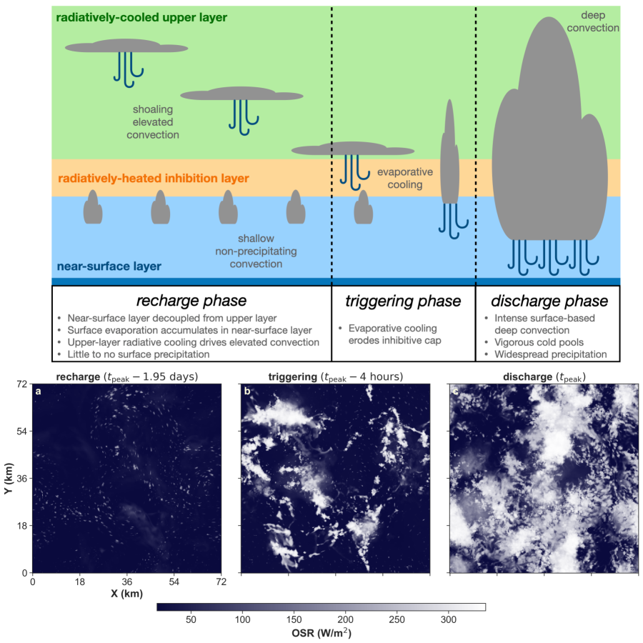
Figure 4: Schematic view of the phases of the relaxation oscillator convective regime. (Bottom) Snapshots of outgoing solar radiation (OSR) during the (a) recharge, (b) triggering, and (c) discharge phases, obtained 1.95 days, 4 hours, and 0 hours before the next hour of peak precipitation ($t_{\mathrm{peak}}$), respectively. These snapshots are from the high-resolution fixed-SST simulation at a surface temperature of 330 K. High values of OSR indicate cloud cover. Neither the graphical width of the phases nor the vertical thickness of the atmospheric layers in this schematic are proportional to the amount of time or space they occupy.

Comparison to parameterized convection

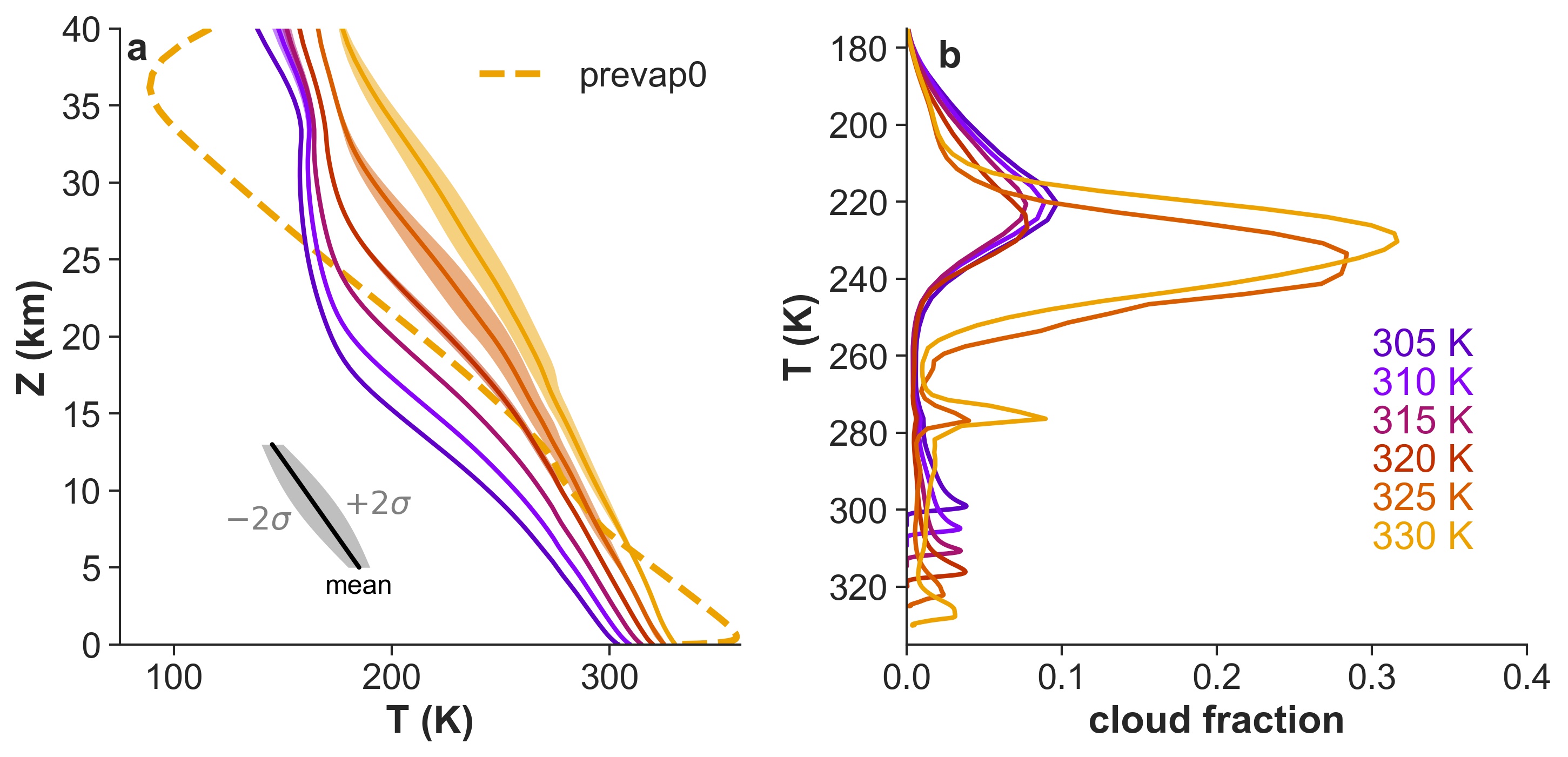
Figure E4: Mean profiles of temperature and cloud fraction. From the fixedSST simulations, profiles of (a) mean temperature and (b) mean cloud fraction (fraction of grid cells with non-precipitating cloud condensate mass fraction greater than 10^-5 kg/kg). In (a), the variability is indicated by the shading, which shows $\pm$2 standard deviations of hourly-mean temperatures at each altitude. In (a), the dashed line shows the mean temperature profile from the simulation without evaporation of precipitating hydrometeors (prevap0) at 330 K.

The convectively-resolved hothouse state has both similarities and differences to prior results from models with parameterized convection. An important difference is that the time-mean temperature profile in our oscillating simulations does not resemble the three-layered structure identified in previous work², ³, ⁴, ⁵, ⁶, with a significant surface-based temperature inversion capped by a deep non-condensing layer and an overlying condensing layer further aloft. Instead, our simulations have tropospheric lapse rates that fall somewhere between the dry and moist adiabats (Fig. E4a), consistent with prior evidence that entraining moist convection sets the temperature profile in the deeply-convecting tropics²⁷, ²⁸. Lacking a significant surface-based temperature inversion, our hothouse climate simulations energetically balance LTRH primarily by the latent cooling of rain evaporation rather than sensible heating of the surface. To further assess the importance of precipitation evaporation in the hothouse climate state, we modified the microphysics parameterization in the model to prevent evaporation of precipitating hydrometeors (rain, snow, and graupel). In contrast to the corresponding case with default microphysics, LTRH in the model without hydrometeor evaporation induces a mean temperature profile closely resembling the three-layered structure from previous work with parameterized convection (Fig. E4a). This suggests that the effects of evaporating hydrometeors on convective triggering and/or tropospheric energetics are critical to hothouse climates. In some global climate models (GCMs), evaporation of precipitation is either neglected or parameterized in a highly idealized manner²⁹, which may be why some previous studies concluded that surface-based inversions are a defining characteristic of hothouse atmospheres³.

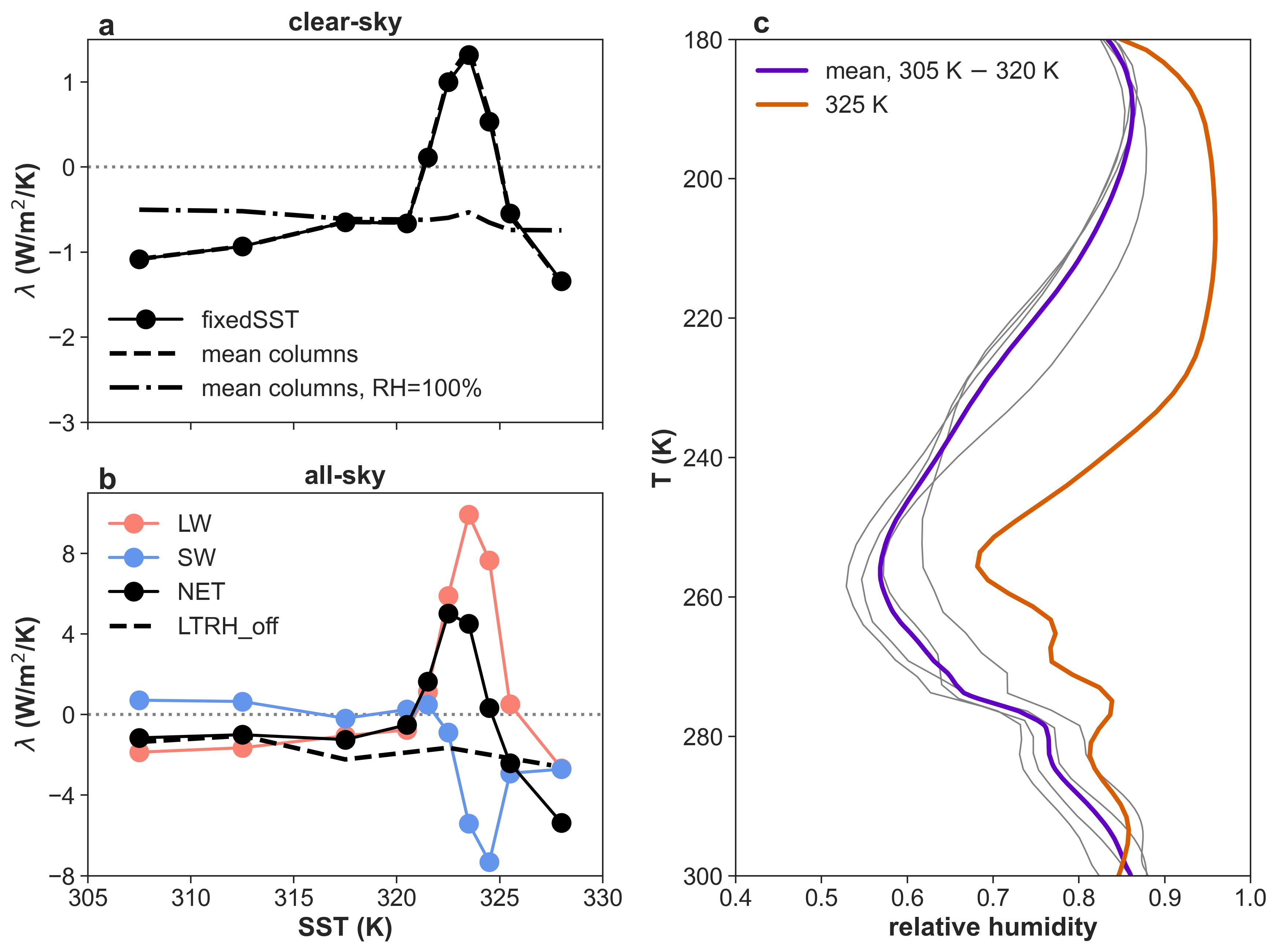
Figure E5: Sign reversal of the climate feedback parameter indicates transient climate instability. The feedback parameter $\lambda$ is defined here as minus the change in net radiative flux at the top-of-atmosphere (TOA) per degree of surface warming (positive downward, so that a negative feedback indicates more radiation escaping to space with warming and hence climate stability, and a positive feedback indicates climate instability; this is often called the “Cess sensitivity”²⁴). We calculated feedbacks using finite differences on a staggered surface temperature grid that interpolates between the surface temperatures of the fixedSST experiment. (a) The solid line shows clear-sky feedbacks calculated for TOA fluxes averaged over the final 100 days of the fixedSST simulations, while the dashed and dot-dashed lines show the feedbacks calculated using the time-mean columns from those simulations with actual or fixed 100% relative humidity profiles, respectively. (b) As in (a), but for the all-sky feedbacks from fixedSST experiments broken down into longwave and shortwave components. The dashed line shows the net all-sky feedback from the final 50 days of the LTRH_off experiment, which does not undergo a steady-to-oscillatory transition and remains stable at all temperatures. (c) Time-mean profiles of relative humidity (RH) in the fixedSST experiments, using temperature within the atmosphere as a vertical coordinate to emphasize the increases in upper-tropospheric relative humidity that occur during the oscillatory transition between 320 and 325 and K. Since the clear-sky climate instability is eliminated by using a fixed relative humidity of 100% (panel a), we attribute the clear-sky climate instability to the increase in upper-tropospheric RH, which lowers spectral emission temperatures and hence OLR.

Our simulations also help clarify prior results from GCMs regarding changes in cloud cover and climate stability in hothouse states. Previous work has suggested that LTRH causes clouds to thin or disappear from the lower troposphere and thicken in a layer of elevated convection in the upper troposphere ³⁰, ³, ⁶. Similarly, in our model elevated condensation and convection during the recharge phase significantly enhance (by a factor of 3–4) the mean upper-tropospheric cloud fraction (Fig. E4b), although shallow clouds do not disappear entirely. A further similarity between our simulations and results from GCMs is the existence of a transient climate instability (i.e., a temporary sign reversal of the climate feedback parameter) during the transition to the new state induced by LTRH⁵, ³, ⁶. In our model, the instability consists of a clear-sky longwave feedback driven by enhanced upper-tropospheric RH, which is significantly amplified by the increase in upper-tropospheric cloud cover in the oscillatory state (Fig. E5). Even for resolved convection, the net cloud radiative effect is sensitive to model details such as the horizontal resolution and microphysics scheme³¹, ³², so the radiative effects of clouds in the oscillatory state deserve additional study. The region of enhanced climate sensitivity associated with the transition to the hothouse state is distinct from the climate sensitivity peak found in our model at lower temperatures³³, the latter of which has been explained in terms of clear-sky feedbacks that operate in the quasi-steady convective regime¹³.

Analogy to spontaneous synchronization

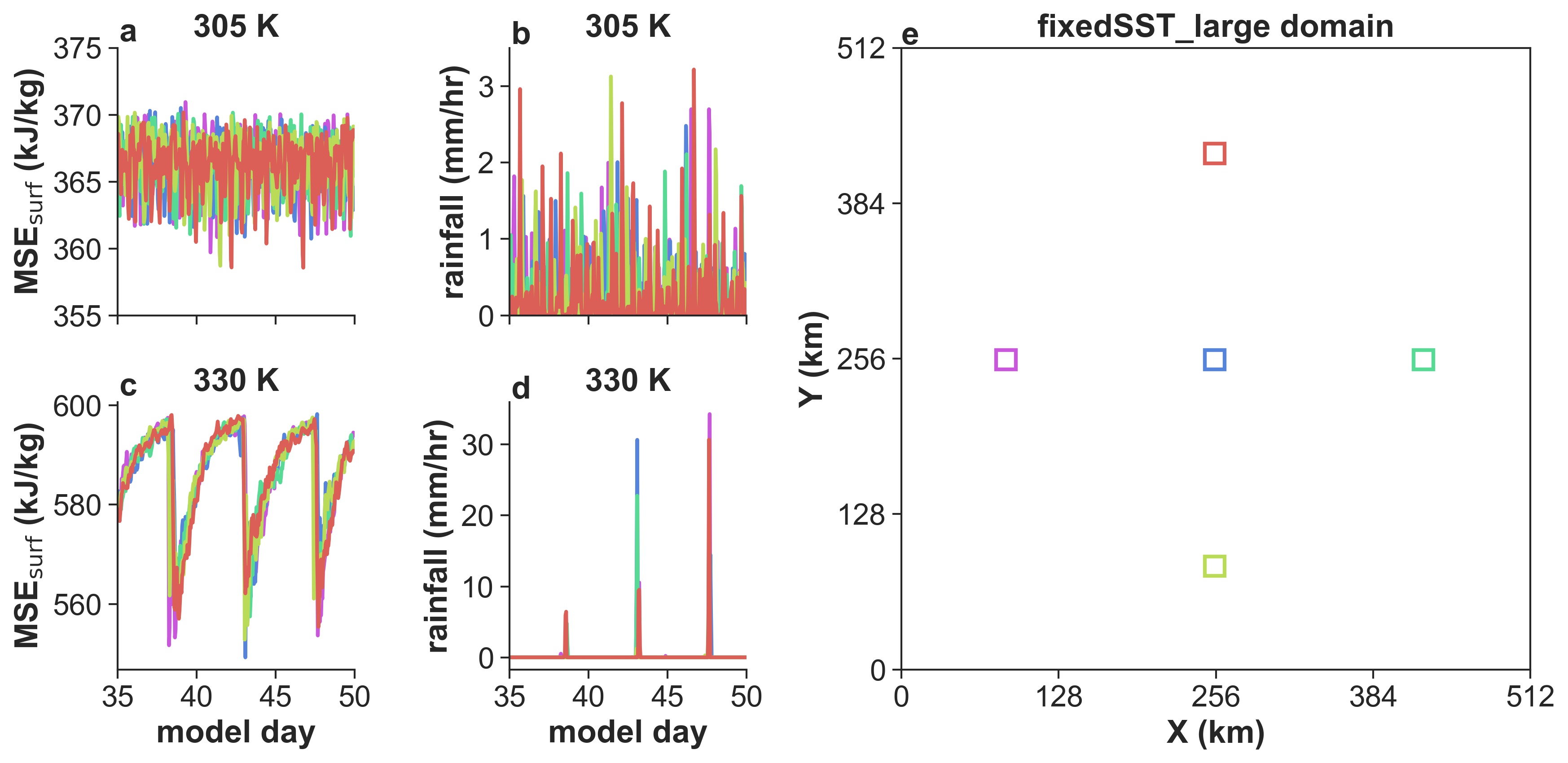
Figure E6: Spatially-separated subdomains exhibit in-phase pulses of convection. Timeseries of (a,c) moist static energy in the lowest model level ($z=12.5$ m; MSE_surf), and (b,d) precipitation rate, averaged over five different subdomains of the fixedSST_large simulations at 305 K (top row) and 330 K (bottom row). The subdomains (color-coded in panel e) each have an area of 256 km² and are located an average of 215 km apart from each other.

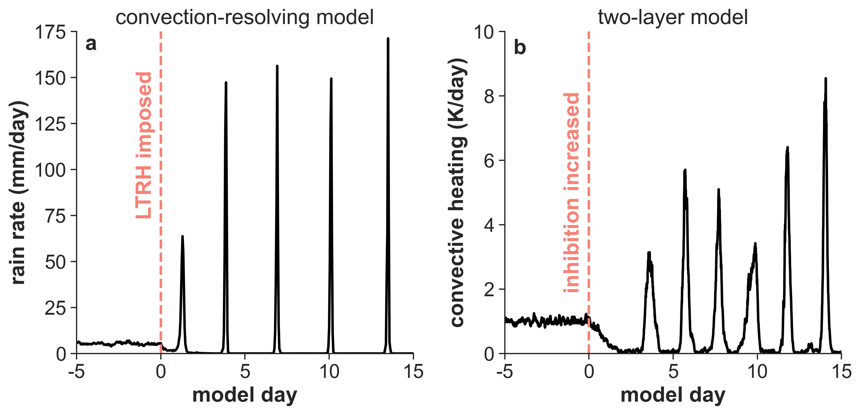
Figure E7: The steady-to-oscillatory transition in the convection-resolving model and the stochastic two-layer model. (a) In the convection-resolving model, the radiative heating profile is switched from cool-climate-type to hothouse-type (LTRH_off to LTRH_on) on model day 0 (the transient_SO simulation). (b) In the two-layer model, the inhibition parameter is increased linearly in time between days 0 and 2 and held fixed thereafter.

Spatial self-aggregation of convection, in which precipitating clouds localize in the horizontal into large and persistent clusters despite spatially-uniform forcing and boundary conditions, has received considerable attention in recent years³⁴. The new relaxation oscillator regime revealed by our work is an analogous state of temporal convective self-aggregation: in the absence of any time-dependent forcing, deep precipitating convection becomes spontaneously synchronized (i.e., temporally localized). The oscillatory state is synchronized in the sense that subdomains separated by hundreds of kilometers exhibit boom-bust cycles of near-surface moist static energy and spikes of precipitation that are nearly in-phase (Fig. E6). The phenomenology of this synchronized atmospheric state closely resembles that of other natural systems that exhibit spontaneous synchronization³⁵, such as mechanical metronomes on a wobbly platform³⁶ and fields of flashing fireflies³⁷. In such systems, the key ingredient that allows for synchronization is a coupling that tends to align the phases of sub-components. In the atmosphere, there are two obvious sources of coupling between spatially-separated sub-domains: 1) gravity waves, which rapidly homogenize temperatures in the free troposphere³⁸, ³⁹, and 2) cold pools, which dynamically trigger additional deep convection in the neighborhood of prior deep convection²³, ²⁴. To investigate this analogy further, we constructed a simple two-layer model of radiative-convective equilibrium that resembles a network of noisy pulse-coupled oscillators³⁵, ¹⁷. Just as in the convection-resolving model, this two-layer model undergoes a steady-to-oscillatory transition when the amount of convective inhibition is increased (Fig. E7).

Discussion

The hothouse convection described here bears similarities to today’s climate in the Great Plains of the central United States, where elevated mixed layers transiently suppress surface-based convection until a triggering mechanism overcomes the inhibition and intense convection ensues⁴⁰, ⁴¹, ⁴². Our results indicate that in hothouse climates, widespread radiatively-generated convective inhibition may shift the spectrum of convective behavior away from the quasi-equilibrium regime⁴³, ⁴⁴ and toward an “outburst” regime more similar to that of the U.S. Great Plains. Since very warm climates have strongly reduced equator-pole temperature gradients³, ⁵, tropical SSTs of between 330–340 K would be accompanied by moist and temperate high latitudes that might support LTRH and the convective outburst regime over a large fraction of Earth’s surface. Nonetheless, an important avenue for future work is to understand how the convective outburst regime described here interacts with large-scale overturning circulations in the tropics, as well as how this regime is expressed at higher latitudes where planetary rotation and seasonal effects play an important role in atmospheric dynamics. Convection-resolving simulations on near-global domains could address these questions, and would also shed light on the prospect of convective synchronization at scales larger than we have investigated here.

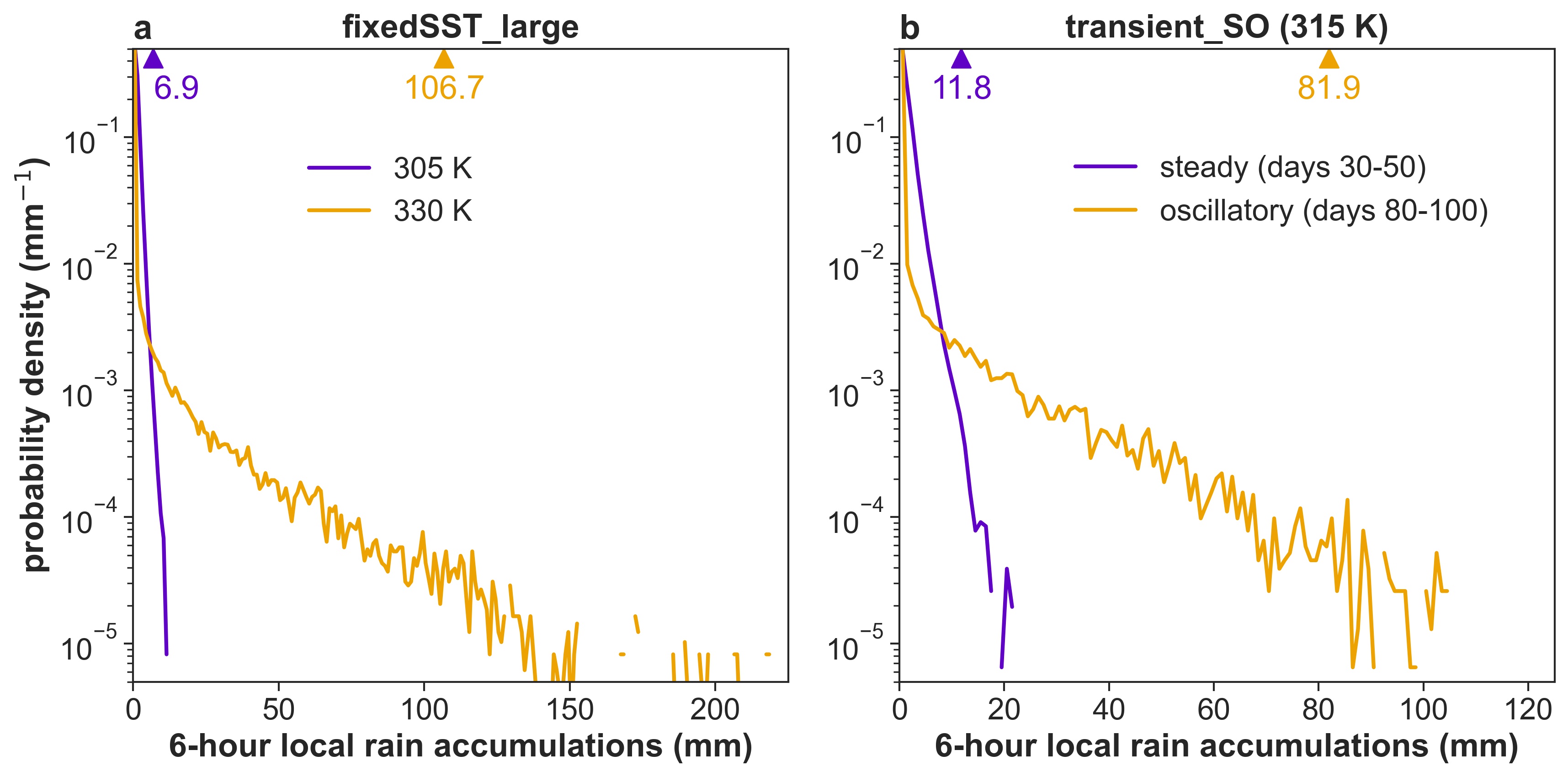
Figure E8: Probability density functions (PDFs) of 6-hour local rain accumulations. The precipitation data are from 20-day periods of (a) the fixedSST_large simulations, and (b) the transient_SO simulation in the steady and oscillatory regime. The PDFs are constructed by first dividing the model domains into watershed-sized subdomains (16$\times$16 km² for fixedSST_large, and 12$\times$12 km² for transient_SO). Precipitation is then accumulated in each subdomain for all 6-hour periods during the 20-day intervals, producing the 6-hour local rain accumulations from which the PDFs are constructed. The 99.9th percentile of each of the PDFs is indicated at the top of each plot.

It is widely recognized that most of the geological work done by precipitation (i.e., erosion, physical weathering, or sediment transport) is associated with large rain events, such that a small number of intense storms play a larger role than many small ones⁴⁵. Although our oscillating simulations have mean precipitation rates similar to their quasi-steady counterparts, local precipitation fluxes are dramatically enhanced in the oscillatory regime. For example, in our large-domain oscillating simulation with an SST of 330 K, watershed-sized areas ($\simeq 1000$ km²) regularly experience 6-hour rain accumulations of several hundred millimeters, comparable to multi-day rainfall totals along the track of landfalling tropical cyclones in the United States⁴⁶. Such large rain accumulations do not occur at all in our quasi-steady simulations (Fig. E8). If lower-tropospheric radiative heating in very warm climates leads to similar oscillatory convective behavior over land, the dramatically increased frequency of intense precipitation events would increase the fraction of rain that is converted to runoff, and presumably cause a significant acceleration of rain-induced surface alteration. Such a shift in rainfall intensity could strengthen the silicate weathering feedback well beyond the upper limit inferred from energetic constraints on the mean precipitation rate⁴⁷, and in principle might even leave an isotopic signature in the geological record⁴⁸, ⁴⁹. While the $\sim$320 K SST threshold for the oscillatory transition in our model is above proxy-based estimates of peak tropical SSTs during the Phanerozoic⁵⁰, such temperatures could have been reached in earlier periods of Earth history, such as the high-CO₂ climates predicted in the aftermath of Neoproterozoic Snowball events ¹⁰.

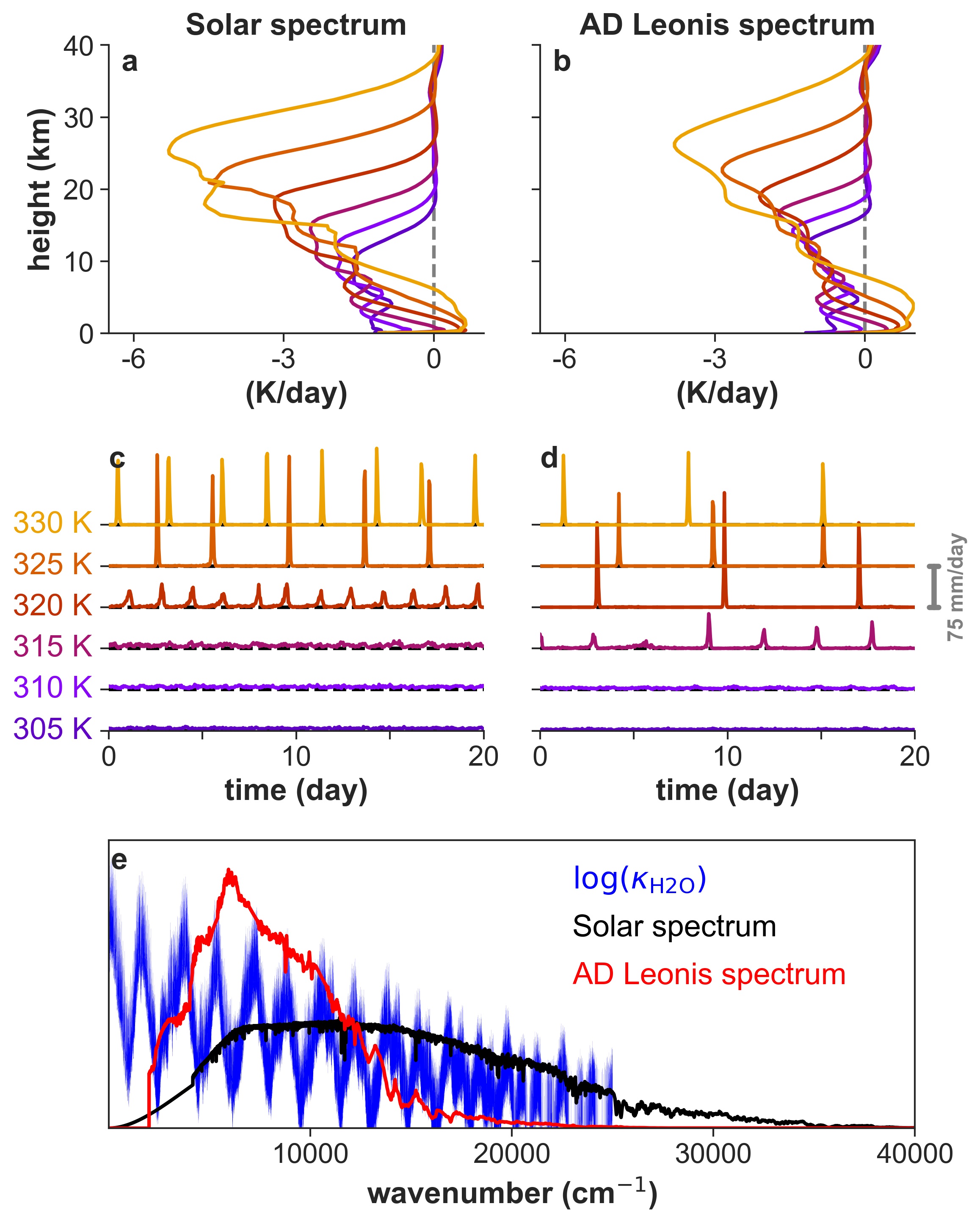
Figure E9: The oscillatory transition occurs more readily for climates instellated by an M-star spectrum. Comparison of tropospheric radiative heating rates (panels a,b) and timeseries of surface precipitation (panels c,d) in fixed-SST simulations with either the solar instellation spectrum or that of the M-star AD Leonis⁴. Panel (e) shows the spectral flux for these two stars (normalized to the same total flux), as well as the logarithm of the H₂O absorption coefficient at a reference temperature and pressure.

Finally, our work has also revealed the potentially significant influence of clouds on top-of-atmosphere radiative fluxes in hothouse climates: in our oscillating simulations, elevated condensation and convection during the recharge phase enhance cloud cover, the planetary albedo, and the longwave greenhouse effect. This could be particularly relevant to tidally-locked planets orbiting M-stars for two reasons: 1) their day-sides receive permanent instellation, and 2) the M-star spectrum is shifted toward the near-infrared. Both of these factors would enhance shortwave absorption by water vapor², and might therefore make the oscillatory convective regime more likely to occur. Indeed, in simulations with an M-star insolation spectrum, we find that the transition to the oscillatory regime occurs at a lower SST than in our standard simulations (Fig. E9). Previous work using a global model with parameterized convection found that lower-tropospheric radiative heating thinned upper-tropospheric cloud decks and led to runaway warming on tidally-locked planets⁴, which runs counter to the trend in high cloud amount we find in our model. These divergent model predictions highlight the importance of investigating the runaway greenhouse transition on Earth-like and tidally-locked planets using global convection-resolving models in the future.

Author contributions

JTS and RWD designed the research. JTS performed the simulations, analyzed the results, and made the figures. The manuscript was written jointly by JTS and RWD. The authors declare no competing interests.

Additional information

Correspondence and requests for materials should be directed to JTS at jacob.t.seeley@gmail.com. Reprints and permissions information is available at www.nature.com/reprints.

Data availability

Input data files and cloud-resolving model output associated with this work is available in a Zenodo repository at the following DOI: 10.5281/zenodo.5117529.

Code availability

Source code for the stochastic two-layer model, processing cloud-resolving model output, and generating figures is available in a Zenodo repository at the following DOI: 10.5281/zenodo.5117529.

Methods

Cloud-resolving model

We use the cloud-resolving model DAM¹⁸ to simulate nonrotating radiative-convective equilibrium (RCE). RCE is an idealization of planetary atmospheres in which radiative and convective heating rates achieve time-mean balance at each altitude².

All DAM simulations were conducted on square, doubly periodic domains with 140 vertical levels between the surface and the free-slip, rigid lid at 60 km. Our vertical grid spacing transitions from $\Delta z=25$ m below an altitude of 650 m, to $\Delta z=500$ m between altitudes of 5.4 and 33 km, and finally to $\Delta z=1000$ m at altitudes above 38 km. Our default horizontal resolution was $\Delta x=\Delta y=2$ km and our default horizontal domain size was $L_{x}=L_{y}=72$ km. The exceptions to this are: 1) the transient_SO and fixedSST_large simulations, which used larger domains of $L_{x}=216$ km and $L_{x}=512$ km, respectively; and 2) the fixedSST_hires simulation, which used a finer horizontal resolution of $\Delta x=250$ m (Extended data table 1). For all but the fixedSST_hires simulations, the model time step was $\Delta t=20$ s, which was sub-stepped to satisfy a CFL condition; for the fixedSST_hires simulations, we used $\Delta t=5$ s. Overall, our model configuration is similar to the “RCE_small” protocol from the RCEMIP project², ³¹ in which DAM participated.

Surface fluxes were modeled with bulk aerodynamic formulae. Specifically, the surface latent and sensible heat fluxes (LHF and SHF) were given by

$$\mathrm{LHF}(x,y)=\rho_{1}(x,y)C_{D}\sqrt{u_{1}(x,y)^{2}+v_{1}(x,y)^{2}+V^{2}}L_{v}\left[q_{\mathrm{s}}^{*}-q_{1}(x,y)\right];$$ (1)

$$\mathrm{SHF}(x,y)=\rho_{1}(x,y)C_{D}\sqrt{u_{1}(x,y)^{2}+v_{1}(x,y)^{2}+V^{2}}c_{p}\left[\mathrm{SST}-T_{1}(x,y)\right],$$ (2)

where $\rho_{1}$, $q_{1}$, $u_{1}$, $v_{1}$, and $T_{1}$ are the density, specific humidity, horizontal winds, and temperature at the first model level, $C_{D}=1.5\times 10^{-3}$ is a drag coefficient, $V=5$ m/s is a background “gustiness”, $L_{v}$ is the latent heat of condensation, $c_{p}$ is the specific heat capacity at constant pressure of moist air, $q_{\mathrm{s}}^{*}$ is the saturation specific humidity at the sea surface temperature and surface pressure. The surface was given a fixed, spectrally-uniform albedo of 0.07.

For simulations with a time-evolving sea surface temperature (CTRL, FSOL, and FCO2), we used a well-mixed slab ocean with horizontally-uniform temperature and heat capacity equal to that of a liquid water layer of depth 1 m. This is a standard approach³³. We used a depth of 1 m to speed the approach to equilibrium; even though this is shallower than Earth’s mixed layer, we have shown that simulations with an infinite heat capacity (fixed-SST simulations) also exhibit the oscillatory regime, which shows that using a shallow ocean does not affect our main results. At each time step, the change in the slab’s internal energy was equated to the sum of an applied ocean heat sink and the net surface enthalpy and radiative fluxes into the ocean. The applied ocean heat sink is necessary because limited-area simulations of the deeply convecting tropics are in a local runaway regime³: the absorbed shortwave radiation exceeds the outgoing longwave radiation by about 100 W/m². In the real atmosphere, this imbalance is accommodated by oceanic and atmospheric heat export, but in a limited-area cloud-resolving model coupled to a slab ocean, the imbalance must be countered by an artificial heat sink applied to the slab ocean or else runaway warming will ensue. We obtained the magnitude of the required heat sink by diagnosing the net enthalpy flux into the ocean averaged over the final 50 days of our standard simulation with a fixed sea surface temperature (fixedSST) of 305 K. This imbalance was 104.9 W/m². Our CTRL simulation (Extended data table 1), which was branched from the end of the fixedSST simulation at 305 K but with the slab ocean and a prescribed ocean heat sink of this magnitude, had a mean SST of 305 K over the ensuing 50 days of integration, confirming that the inclusion of this heat sink closed the column (ocean+atmosphere) heat budget. The solar- and CO₂-induced warming experiments (FSOL and FCO2) also include this same ocean heat sink.

For all simulations, domain-mean horizontal winds were nudged to zero on a timescale of 6 hours to avoid the development of stratospheric jets. To minimize artificial gravity wave reflection off the model’s rigid lid, a sponge layer was also included at altitudes above 40 km in which damping was applied to all three components of the wind field.

Additional details of the DAM simulations conducted for this work are summarized in Extended data table 1.

Table M1: Summary of key aspects of the suite of DAM simulations conducted for this work.

Radiative transfer modeling

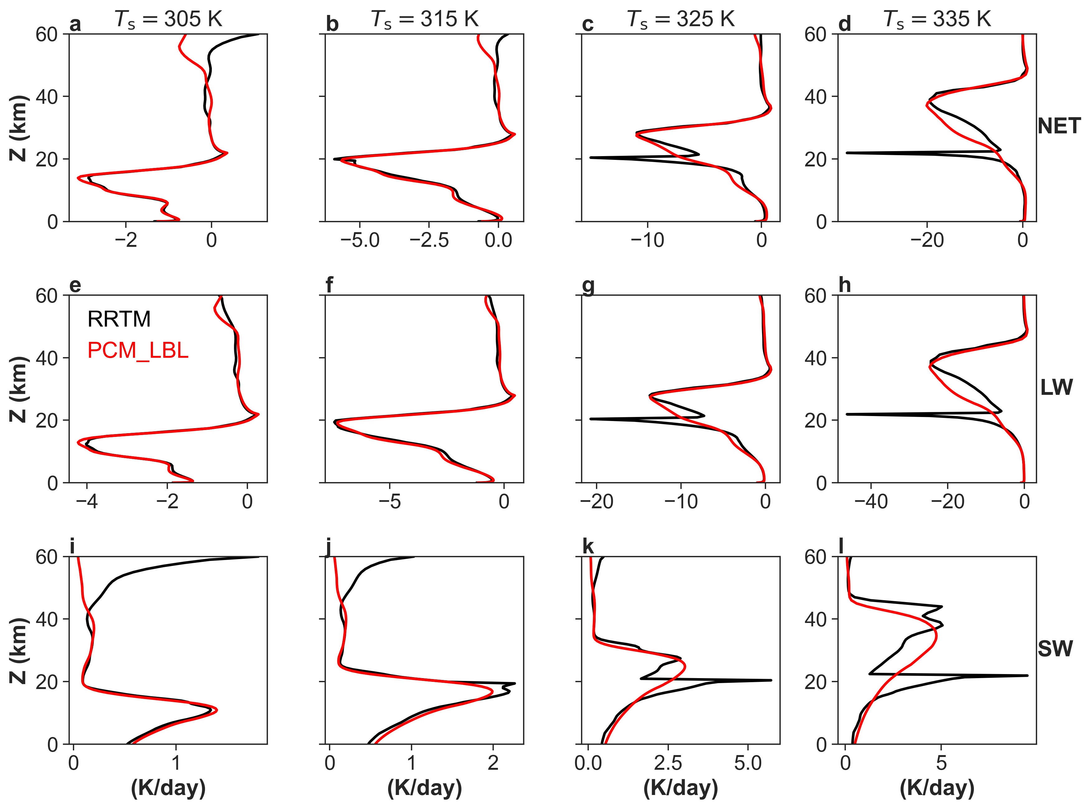
Figure E1: Errors in clear-sky RRTM radiative heating rates are corrected by using line-by-line radiative transfer. Comparison of net (LW+SW; panels a–d), longwave (LW; panels e–h), and shortwave (SW; panels i–l) radiative heating rates as computed by RRTM (black) and PCM_LBL (red). The heating rates are computed for moist-adiabatic temperature-pressure profiles with surface temperatures ranging from 305 K to 335 K in 10-K increments (columns, left to right). All columns have a surface pressure of 101325 Pa, 75% tropospheric relative humidity, 400 ppm CO₂, and an isothermal stratosphere at 160 K. Note that the discontinuous heating rates calculated by RRTM for the warmer atmospheres (around 20 km altitude) do not appear in the PCM_LBL results.

For shortwave and longwave radiative transfer, DAM is coupled to the fully interactive Rapid Radiative Transfer Model (RRTM)⁵, ⁶. RRTM is a correlated-$k$ code that prioritizes computational efficiency and is validated for atmospheric conditions close to those of contemporary Earth. However, RRTM can produce unphysical results for the very warm atmospheres that are our focus. Figure E1 shows clear-sky longwave and shortwave radiative heating rates calculated by RRTM for a series of increasingly warm moist-adiabatic soundings. The unphysical discontinuities in heating rate at around 20 km altitude in the warmer soundings appear to be due to the fact that RRTM uses different lookup tables and approximations above and below a hard-coded pressure. For cooler climates, this transition pressure occurs safely in the stratosphere and there is no heating rate discontinuity, but in warmer climates the transition pressure lands in the middle of the much taller troposphere.

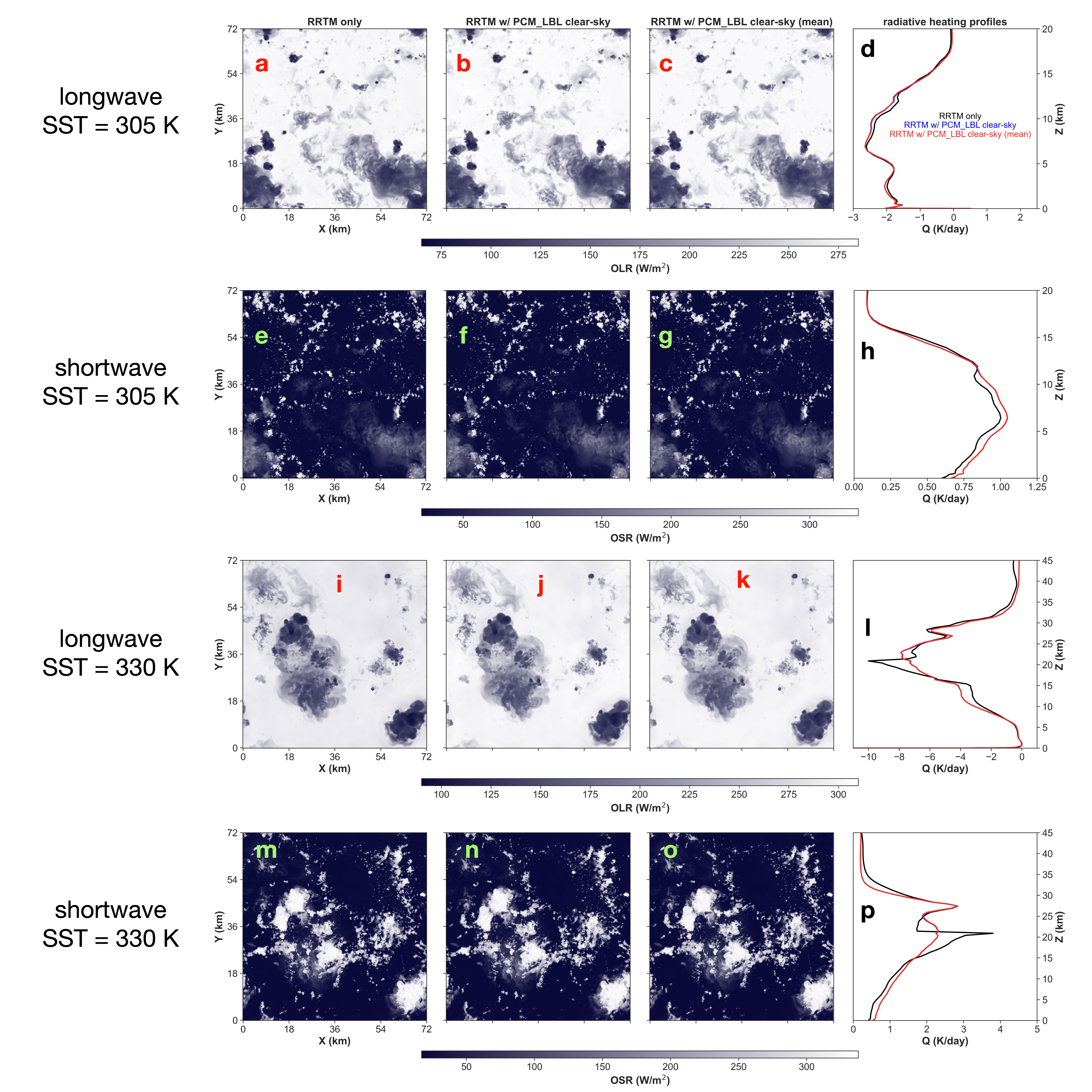
Figure E2: Top-of-atmosphere radiative fluxes and heating rates from DAM snapshots. (a–c) Outgoing longwave radiation (OLR) from a snapshot from the fixedSST_hires DAM simulation with a surface temperature of 305 K, computed by three different combinations of radiative transfer codes and approximations. Panel (a) is from RRTM alone, panel (b) shows the result of swapping out the clear-sky radiative fluxes from RRTM with those calculated by PCM_LBL, and panel (c) shows the result of swapping out each column’s clear-sky radiative fluxes for those calculated by PCM_LBL for the horizontal-mean column, which is the approach taken for the simulations associated with this work. Panel (d) shows the horizontal-mean longwave radiative heating rates for this snapshot. (e–h) As in (a–d), but for absorbed shortwave radiation (ASR). (i–p) As in (a–h), but for a snapshot from the simulation with a surface temperature of 330 K.

To obtain more realistic radiative heating rates in very warm atmospheres, we coupled DAM to a line-by-line radiation scheme known as PCM_LBL⁷. This code simply solves the radiative transfer equations directly as a function of wavenumber, on a fine enough spectral grid that the heating rates in our atmospheres converge. Figure E1 shows that the clear-sky radiative heating rates calculated by PCM_LBL closely match those of RRTM in current tropical conditions, and do not suffer from any unphysical discontinuities in heating rate in warm atmospheres. However, PCM_LBL is a clear-sky code, so to retain the effect of cloud-radiative interactions in our simulations, we took a hybrid approach: at every call to the radiation scheme (every 200 s), we swapped out the clear-sky radiative fluxes calculated by RRTM for those calculated by PCM_LBL for the horizontal-mean clear-sky column, while retaining the cloud-radiative effects calculated by RRTM. Using the horizontal-mean clear-sky column neglects variations in radiative heating rates due to horizontal variations in water vapor. However, sensitivity tests (not shown) indicated that this had a negligible effect on our simulation results, with differences in time-mean cloud-radiative effect of order 1 W/m². Figure E2 shows that this approach captures cloud-radiative effects closely. These effects are the dominant source of variability in top-of-atmosphere fluxes and atmospheric heating rates in our simulations. We also note that our approach to radiation is justified by the LTRH_on experiment suite (Extended data table 1), which shows that the transition to the oscillatory convective regime due to lower-tropospheric radiative heating does not depend on the details of cloud-radiative interactions. We validate and fully describe our radiative transfer modeling with PCM_LBL below.

Our longwave calculations with PCM_LBL covered the wavenumber range from 0–4000 cm^-1, while our shortwave calculations covered 0–50000 cm^-1. The spectral resolution for both channels was 0.1 cm^-1. While this spectral resolution does not resolve the cores of lines at very low (upper-stratospheric) pressures, sensitivity tests showed that further increases in resolution yielded negligible changes to the radiative fluxes and heating rates in the troposphere, which is our focus. Similar convergence was also found in previous work ⁷, ⁸. At each wavenumber, the monochromatic radiative transfer equation was solved using an approach described in previous work⁹, which uses the layer optical depth weighting scheme¹⁰ to ensure accurate model behavior in strongly-absorbing portions of the spectrum. To compute radiative fluxes, we used the two-stream approximation with first-moment Gaussian quadrature ¹⁰.

PCM_LBL uses lookup tables of absorption coefficients on a pressure-temperature grid that covers the range of atmospheric conditions encountered in the model evolution, and interpolates to the current horizontal-mean atmospheric state at each vertical model level. Our pressure-temperature grid had a total of 20 pressure levels, with 10 levels spaced linearly in pressure between 110000 Pa and 10000 Pa, and 10 levels spaced logarithmically between 10000 Pa and 0.1 Pa. On each pressure level, absorption coefficients were evaluated at a set of 20 temperatures (spaced 10 K apart) that bracket the conditions encountered in the model evolution. To generate the absorption-coefficient lookup tables for H₂O and CO₂ from the HITRAN2016 database ¹¹, we used the RFM, a contemporary line-by-line model ¹². Both PCM_LBL and RRTM use MT-CKD to calculate the water vapor continuum ¹³.

For shortwave radiation, we modeled gaseous absorption only, which is appropriate for clear skies at wavelengths where Rayleigh scattering is not important. In reality, Rayleigh scattering in clear skies enhances the planetary albedo, but this process is important at significantly shorter wavelengths than the near-infrared wavelengths absorbed by H₂O. Therefore, the inclusion of Rayleigh scattering would introduce a small offset in the relationship between insolation and equilibrated surface temperature in our model, which would simply be absorbed into the oceanic heat sink. Our shortwave radiation setup differs for our M-star simulations (MSTAR) and for our Earth-like experiment configurations (all other simulations with interactive radiation). For our Earth-like configurations, we used top-of-atmosphere downwelling spectral solar flux data¹⁴ normalized to our specified values of the solar constant. For the MSTAR experiment, we used spectral instellation data from the M-star Ad Leonis B⁴. We did not include a diurnal cycle of insolation; for our Earth-like configurations, the cosine of the solar zenith angle was set to its insolation-weighted average during the diurnal cycle at the equator on 1 January, yielding a zenith angle of 43.75^∘. With a contemporary solar constant of 1366 W/m², this yields a downwelling shortwave flux at top-of-atmosphere of 413.13 W/m². This shortwave insolation was used for all Earth-like simulations with interactive radiation except for the FSOL simulation, which used a solar constant larger by 10%. For our MSTAR experiment, we set the cosine of the solar zenith angle to its instellation-weighted (dayside) mean, yielding a zenith angle of 48.19^∘, and used a stellar constant of 800 W/m².

Microphysics parameterizations

The default microphysics scheme in DAM is known as the Lin-Lord-Krueger parameterization ¹⁵, ¹⁶, ¹⁷. The LLK parameterization is a bulk scheme with six water classes (vapor, cloud liquid, cloud ice, rain, snow, and graupel). Almost all of our DAM simulations were conducted with this microphysics scheme; however, to test the robustness of our main results to microphysics, we also conducted fixed-SST simulations at 305 K and 330 K (the fixedSST_sm suite; Extended data table 1) using a highly simplified microphysics scheme that has been described in previous work^{18, 19}; we also describe this simplified scheme below. Additionally, the “prevap0” simulations used the LLK microphysics parameterization, but with all evaporation of precipitating hydrometeors (rain, snow, and graupel) set to zero.

In the simplified microphysics scheme, there is no ice phase (i.e., water is modeled as a two-phase substance, with latent heat associated with phase change between vapor and liquid only). Accordingly, only three bulk classes of water substance are modeled: vapor, non-precipitating cloud liquid, and rain, with associated mass fractions $q_{\mathrm{v}}$, $q_{\mathrm{c}}$, and $q_{\mathrm{r}}$, respectively. Microphysical transformations between vapor and cloud condensate are handled by a saturation adjustment routine, which prevents relative humidity from exceeding 100% (i.e., abundant cloud condensation nuclei are assumed to be present) and evaporates cloud condensate in subsaturated air. Conversion of non-precipitating cloud condensate to rain is modeled as autoconversion according to

$$a=-q_{\mathrm{c}}/\tau_{\mathrm{a}},$$ (3)

where $a$ (s^-1) is the sink of cloud condensate from autoconversion and $\tau_{\mathrm{a}}$ (s) is an autoconversion timescale. We use $\tau_{\mathrm{a}}=25$ minutes, which was found in prior work to produce a similar mean cloud fraction profile as the LLK microphysics scheme¹⁹. We did not set an autoconversion threshold for $q_{\mathrm{c}}$. Furthermore, rain is given a fixed freefall speed of 8 m/s in this simplified microphysics scheme. When rain falls through subsaturated air, it is allowed to evaporate according to

$$e=(q_{\mathrm{v}}^{*}-q_{\mathrm{v}})/\tau_{\mathrm{r}},$$ (4)

where $e$ (s^-1) is the rate of rain evaporation, $q_{\mathrm{v}}^{*}$ is the saturation specific humidity, and $\tau_{\mathrm{r}}$ (s) is a rain-evaporation timescale. We set $\tau_{\mathrm{r}}=50$ hours, which was found in prior work to produce a tropospheric relative humidity profile similar to that of the LLK scheme¹⁹.

Near-surface tracer

In the oscillatory state, convective mass flux can be divided into two categories: updrafts that emanate from the near-surface layer ($z<1$ km), and updrafts that originate from higher in the troposphere. To discriminate between these two categories, we employed a passive tracer that measures what fraction of dry air in an updraft was recently advected from below a certain height (here, 1 km)²⁰ and. We denote this tracer’s mixing ratio as $\chi_{\mathrm{ns}}$. At every model time step, $\chi_{\mathrm{ns}}$ was set to 1 at altitudes below 1 km, and set to zero above that height except in the “vicinity” of cloudy updrafts. We define cloudy updrafts as grid cells that have vertical velocity $w\geq 0.5$ m/s and non-precipitating cloud condensate $q_{n}\geq 10^{-2}$ g/kg, and their “vicinity” as a cube of side length 7 grid cells centered on the updraft²⁰. Cloudy-updraft grid cells in which this tracer has a value of 0 contain no air that originated in the near-surface layer, so we assigned mass flux with a mean value of $\chi_{\mathrm{ns}}=0$ during our 5-minute sampling interval to the “elevated” category, and assigned the remainder to the “surface-based” category. This is an overly stringent definition of elevated convection, since any amount of surface-based convection that occurs at a certain altitude within the 5-minute sampling interval will knock other (potentially elevated) updrafts out of the “elevated” category. Nevertheless, we still identify a large amount of elevated convection in Figure 3a of the main text.

Simulations with other cloud-resolving models

In addition to our simulations with DAM, we also conducted simulations with two other cloud-resolving models: the System for Atmospheric Modeling (SAM)²¹ and the Cloud Model 1 (CM1)²². With each model, we conducted fixed-SST simulations at 305 K and 325 K, initialized with soundings from the corresponding fixedSST DAM simulation.

For our SAM simulations, we used a domain of horizontal dimension 144 km with 2 km resolution. We used the same vertical grid as used for our DAM simulations, but extended to 64 km (for a total of 144 levels in the vertical) to satisfy parallelization requirements in SAM. We used a time-step of 10 s. The radiation scheme was RRTM, and the microphysics scheme was SAM’s 1-moment scheme. We ran each simulation for 100 days.

For our CM1 simulations, we used a domain of horizontal dimension 72 km with 2 km resolution, and 100 vertical levels with a stretched grid (50 m resolution at altitudes below 650 m, and 500 m resolution at altitudes above 5600 m). We used a time-step of 20 s. The radiation scheme was RRTMG, and we used the Morrison double-moment microphysics scheme²³. We ran each simulation for 150 days.

Stochastic two-layer model

To explore the analogy between the oscillatory convective regime and the phenomenon of spontaneous synchronization³⁵, we constructed a simple two-layer model of RCE that resembles a network of noisy pulse-coupled oscillators. In this model, the two layers represent the near-surface layer and the upper troposphere. Each layer has a thermodynamic state variable $T$ whose time-evolution is governed by a combination of surface fluxes and convection (in the case of the lower layer) or radiation and convection (in the case of the upper layer). The upper layer is assumed to be well-mixed (with a single $T$), whereas the lower layer is divided into $N=nx\times ny$ cells arranged in a 2-dimensional, doubly-periodic lattice, each with its own $T$. Each lower-layer cell is coupled to the surface by a relaxation to a surface thermodynamic state of $T_{\mathrm{s}}=0$. (The choice of $T_{\mathrm{s}}$ is arbitrary as it simply adds an offset to the temperatures of the other layers). The two layers are also coupled by convection, which we model as a stochastically-triggered relaxation process that we describe in more detail below.

The governing equation for the upper layer temperature $T_{u}$ is:

$$\frac{dT_{u}}{dt}=Q+\frac{1}{N}\sum_{i,j}M_{ij},$$ (5)

where $Q$ (K/day) is the radiative heating rate in the upper troposphere (negative values indicate cooling) and $M_{ij}$ (K/day) is the deep-convective heating rate from boundary layer cell $(i,j)$. The governing equation for the lower layer cell temperatures $T_{ij}$ is

$$\frac{dT_{ij}}{dt}=-T_{ij}/\tau_{\mathrm{s}}-M_{ij},$$ (6)

where $\tau_{\mathrm{s}}$ is the surface-flux timescale. Note that, due to our choice of $T_{\mathrm{s}}=0$, $T_{ij}$ is negative (i.e., the surface-flux term acts as a relaxation to the surface temperature of 0).

We model convective triggering and heating as stochastic processes. The generation of a convective event proceeds in three steps: 1) testing if an event is triggered; 2) determining the magnitude of the event; and 3) determining if the event can overcome an externally-specified convective inhibition parameter. For the first step, convective triggering in each grid cell is assumed to behave as a Poisson process, which is a generic representation of events that are rare and independent but that occur at an expected rate. Accordingly, the probability of convective triggering in a small time step $\Delta t$ is given by $\exp(-\lambda\Delta t)$, where $\lambda$ (day^-1) is the expected rate of convective triggering. If convection is triggered, the second step determines the size of the event by drawing an inverse timescale $\alpha_{ij}$ (day^-1) from an exponential distribution:

$$\mathrm{P}(\alpha_{ij})=\frac{1}{\beta_{ij}}\exp(-\alpha_{ij}/\beta_{ij}),$$ (7)

for scale parameter $\beta_{ij}$. Hence larger inverse timescales, which correspond to larger convective mass fluxes/heating rates, are less common than smaller events. To represent the fact that downdrafts from neighboring convection generate larger convective plumes with lower bulk entrainment rates and larger heating rates²⁵, we made the scale parameter $\beta_{ij}$ linearly dependent on the convective heating rate in nearby grid cells:

$$\beta_{ij}=\beta_{0}\left(1+\frac{M_{\mathrm{neighbors}}}{M_{0}}\right),$$ (8)

where $M_{\mathrm{neighbors}}$ is the convective heating rate summed over the “neighborhood” of the lower-layer cell, which we specify below. The parameter $M_{0}$ (K/day), as well as the chosen size of the neighborhood of each lower-layer cell, together set the sensitivity of $\beta_{ij}$ to neighboring convection.

Finally, once the size of the triggered event is determined, $\alpha_{ij}$ is compared to the inhibition parameter $I$ (day^-1). $I$ functions as a cutoff scale: the triggered event only occurs if $\alpha_{ij}>I$. In the case of a triggered event at time $t^{*}_{ij}$ that overcomes the inhibition, the convective heating rate in cell $(i,j)$ is set as

$$M_{ij}(t)=\begin{cases}\max\left[\alpha_{ij}(T_{ij}-T_{u}),0\right],&\text{for}\quad t^{*}_{ij}\leq t<t^{*}_{ij}+\tau_{\mathrm{c}}\\ 0,&\text{otherwise},\end{cases}$$ (9)

where $\tau_{\mathrm{c}}$ is the duration of convective events. We do not allow additional convective events to trigger when there is an ongoing event. While heuristic, this model captures some of the basic features of the convective feedbacks that occur in the full RCE simulations.

The two-layer model equations are integrated numerically with a simple forward-difference Euler method. We used parameter values $Q=-1$ K/day, $\tau_{\mathrm{s}}=1$ day, $\tau_{\mathrm{c}}=1$ hour, $\lambda=12$ day^-1, $\beta_{0}=1$ day^-1 and $M_{0}=1$ K/day. We defined the neighborhood of each grid cell as a square of side length 9 grid cells centered on cell $(i,j)$, and we used a grid of size $nx=ny=50$ and a time step of 10 minutes. We checked model convergence by halving the time step twice (to 5 and 2.5 minutes) and found very similar results in both cases.

For Figure E7, we first integrated the model for 15 days with a low value of inhibition $I=1$ day^-1, then integrated the model for two days while linearly increasing $I$ to 6 day^-1 (representing the buildup of inhibition after radiative heating is switched on in the transient_SO simulation), and finally integrated the model for another 15 days with $I$ held fixed at the larger value.

Extended data video

An extended data video is available at the following URL: https://youtu.be/NALhYFiaeos.

Extended data video 1 is an animation of DAM model output from the fixed-SST simulation at 330 K (from our fixedSST_hires suite; Extended data table 1). Each frame in the video consists of 6 panels showing, from top to bottom and left to right: buoyancy in the near-surface layer, wind speed in the near-surface layer, outgoing solar radiation, temperature anomaly in the near-surface layer, specific humidity anomaly in the near-surface layer, and accumulated rainfall over the preceding 6 hours. Anomalies are calculated with respect to the horizontal- and time-mean. The sampling interval between frames is 15 minutes, and the animations cover 7 days of model time.

References

- 1 Steffen, W. et al. Trajectories of the earth system in the anthropocene. Proceedings of the National Academy of Sciences 115, 8252–8259 (2018).
- 2 Wordsworth, R. D. & Pierrehumbert, R. T. Water loss from terrestrial planets with CO2-rich atmospheres. The Astrophysical Journal 778 (2013).
- 3 Wolf, E. T. & Toon, O. B. The evolution of habitable climates under the brightening Sun. Journal of Geophysical Research: Atmospheres 120, 5775–5794 (2015).
- 4 Kopparapu, R. K. et al. The inner edge of the habitable zone for synchronously rotating planets around low-mass stars using general circulation models. The Astrophysical Journal 819 (2016).
- 5 Popp, M., Schmidt, H. & Marotzke, J. Transition to a moist greenhouse with CO2 and solar forcing. Nature Communications 7 (2016).
- 6 Wolf, E. T., Haqq-Misra, J. & Toon, O. B. Evaluating climate sensitivity to CO2 across Earth’s history. Journal of Geophysical Research: Atmospheres 123, 11,861–11,874 (2018).
- 7 Snyder, C. W. Evolution of global temperature over the past two million years. Nature 538, 226–228 (2016).
- 8 Sleep, N. H. The Hadean-Archaean Environment. Cold Spring Harb. Perspect. Biol. 1–15 (2010).
- 9 Charnay, B., Le Hir, G., Fluteau, F., Forget, F. & Catling, D. C. A warm or a cold early Earth? New insights from a 3-D climate-carbon model. Earth and Planetary Science Letters 474, 97–109 (2017).
- 10 Pierrehumbert, R., Abbot, D., Voigt, A. & Koll, D. Climate of the Neoproterozoic. Annual Review of Earth and Planetary Sciences 39, 417–460 (2011).
- 11 Goldblatt, C. & Watson, A. J. The runaway greenhouse: Implications for future climate change, geoengineering and planetary atmospheres. Philosophical Transactions of the Royal Society A: Mathematical, Physical and Engineering Sciences 370, 4197–4216 (2012).
- 12 Koll, D. D. B. & Cronin, T. W. Earth’s outgoing longwave radiation linear due to H2O greenhouse effect. Proceedings of the National Academy of Sciences of the United States of America 115, 10293–10298 (2018).
- 13 Seeley, J. T. & Jeevanjee, N. H2O windows and CO2 radiator fins: A clear-sky explanation for the peak in equilibrium climate sensitivity. Geophysical Research Letters 48, 1–12 (2021).
- 14 Yang, J., Cowan, N. B. & Abbot, D. S. Stabilizing cloud feedback dramatically expands the habitable zone of tidally locked planets. The Astrophysical Journal Letters 45 (2013).
- 15 Sergeev, D. E. et al. Atmospheric convection plays a key role in the climate of tidally-locked terrestrial exoplanets: insights from high-resolution simulations. The Astrophysical Journal 894 (2020).
- 16 Lefèvre, M., Turbet, M. & Pierrehumbert, R. 3D convection-resolving model of temperate, tidally locked exoplanets. The Astrophysical Journal 913, 101 (2021).
- 17 See methods for futher details .
- 18 Romps, D. M. The Dry-Entropy Budget of a Moist Atmosphere. Journal of the Atmospheric Sciences 65, 3779–3799 (2008).
- 19 Wang, D. Relaxation Oscillators and Networks. Wiley Encyclopedia of Electrical and Electronics Engineering 18, 396–405 (1999).
- 20 Ginoux, J. M. & Letellier, C. Van der Pol and the history of relaxation oscillations: Toward the emergence of a concept. Chaos 22 (2012). 1408.4890.
- 21 Pendergrass, A. G. & Hartmann, D. L. The Atmospheric Energy Constraint on Global-Mean Precipitation Change. Journal of Climate 27, 757–768 (2014).
- 22 Jeevanjee, N. & Romps, D. M. Mean precipitation change from a deepening troposphere. Proceedings of the National Academy of Sciences 115, 11465–11470 (2018).
- 23 Torri, G., Kuang, Z. & Tian, Y. Mechanisms for convection triggering by cold pools. Geophysical Research Letters 42, 1–8 (2015).
- 24 Jeevanjee, N. & Romps, D. M. Effective buoyancy, inertial pressure, and the mechanical generation of boundary layer mass flux by cold pools. Journal of the Atmospheric Sciences 72, 3199–3213 (2015).
- 25 Feng, Z. et al. Mechanisms of convective cloud organization by cold pools over tropical warm ocean during the AMIE/DYNAMO field campaign. Journal of Advances in Modeling Earth Systems 7, 357–381 (2015).
- 26 Torri, G. & Kuang, Z. On cold pool collisions in tropical boundary layers. Geophysical Research Letters 46, 399–407 (2019).
- 27 Singh, M. S. & O’Gorman, P. A. Influence of entrainment on the thermal stratification in simulations of radiative-convective equilibrium. Geophysical Research Letters 40, 4398–4403 (2013).
- 28 Seeley, J. T. & Romps, D. M. Why does tropical convective available potential energy (CAPE) increase with warming? Geophysical Research Letters 42, 1–9 (2015).
- 29 Zhao, M. Uncertainty in model climate sensitivity traced to representations of cumulus precipitation microphysics. Journal of Climate 29, 543–560 (2016).
- 30 Popp, M., Schmidt, H. & Marotzke, J. Initiation of a runaway greenhouse in a cloudy column. Journal of the Atmospheric Sciences 72, 141006071034003 (2014).
- 31 Wing, A. A. et al. Clouds and convective self-aggregation in a multimodel ensemble of radiative-convective equilibrium simulations. Journal of Advances in Modeling Earth Systems 12, 1–38 (2020).
- 32 Becker, T. & Wing, A. A. Understanding the extreme spread in climate sensitivity within the radiative-convective equilibrium model intercomparison project. Journal of Advances in Modeling Earth Systems 12 (2020).
- 33 Romps, D. M. Climate sensitivity and the direct effect of carbon dioxide in a limited-area cloud-resolving model. Journal of Climate 33, 3413–3429 (2020).
- 34 Wing, A. A., Emanuel, K., Holloway, C. E. & Muller, C. Convective self-aggregation in numerical simulations: A review. Surveys in Geophysics 38, 1173–1197 (2017).
- 35 Mirollo, R. E. & Strogatz, S. H. Synchronization of pulse-coupled biological oscillators. SIAM Journal on Applied Mathematics 50, 1645–1662 (1990).
- 36 Pantaleone, J. Synchronization of metronomes. American Journal of Physics 70, 992–1000 (2002).
- 37 Buck, J. & Buck, E. Biology of synchronous flashing of fireflies. Nature 211, 562–564 (1966).
- 38 Bretherton, C. S. & Smolarkiewicz, P. K. Gravity waves, compensating subsidence, and detrainment around cumulus clouds. Journal of the Atmospheric Sciences 46 (1989).
- 39 Edman, J. P. & Romps, D. M. Beyond the rigid lid: Baroclinic modes in a structured atmosphere. Journal of the Atmospheric Sciences 74, 3551–3566 (2017).
- 40 Carlson, T. N., Benjamin, S. G. & Forbes, G. S. Elevated mixed layers in the regional severe storm environment: conceptual model and case studies. Monthly Weather Review 11 (1983).
- 41 Schultz, D. M., Richardson, Y. P., Markowski, P. M. & Doswell, C. A. Tornadoes in the central United States and the “clash of air masses”. Bulletin of the American Meteorological Society 95, 1704–1712 (2014).
- 42 Agard, V. & Emanuel, K. Clausius–Clapeyron scaling of peak CAPE in continental convective storm environments. Journal of the Atmospheric Sciences 74, 3043–3054 (2017).
- 43 Arakawa, A. & Schubert, W. H. Interaction of a cumulus cloud ensemble with the large-scale environment, Part I. Journal of the Atmospheric Sciences 31 (1974).
- 44 Raymond, D. Boundary layer quasi-equilibrium (BLQ). The Physics and Parameterization of Moist Atmospheric Convection 387–397 (1997).
- 45 Melosh, J. Water. In Planetary Surface Processes (Cambridge University Press, 2011).
- 46 Villarini, G., Smith, J. A., Baeck, M. L., Marchok, T. & Vecchi, G. A. Characterization of rainfall distribution and flooding associated with U.S. landfalling tropical cyclones: Analyses of Hurricanes Frances, Ivan, and Jeanne (2004). Journal of Geophysical Research Atmospheres 116 (2011).
- 47 Graham, R. J. & Pierrehumbert, R. Thermodynamic and energetic limits on continental silicate weathering strongly impact the climate and habitability of wet, rocky worlds. The Astrophysical Journal 896, 115 (2020).
- 48 Dansgaard, W. Stable isotopes in precipitation. Tellus 16, 436–468 (1964).
- 49 Pausata, F. S., Battisti, D. S., Nisancioglu, K. H. & Bitz, C. M. Chinese stalagmite 18 O controlled by changes in the indian monsoon during a simulated heinrich event. Nature Geoscience 4, 474–480 (2011).
- 50 Frieling, J. et al. Extreme warmth and heat-stressed plankton in the tropics during the Paleocene-Eocene Thermal Maximum. Science Advances 3 (2017).
Acknowledgements
We are grateful to the authors of the cloud-resolving models used in this work: David Romps, Marat Khairoutdinov, and George Bryan. We also thank Anu Dudhia for sharing with us the Reference Forward Model. The authors thank Xin Wei for conducting exploratory simulations with SAM. JTS thanks Nadir Jeevanjee, Aaron Match, Nathaniel Tarshish, and Zhiming Kuang for discussions.

References

- 1
- 2 Wing, A. A. et al. Radiative-convective equilibrium model intercomparison project. Geoscientific Model Development Discussions 11, 1–34 (2017).
- 3 Romps, D. M. Response of tropical precipitation to global warming. Journal of the Atmospheric Sciences 68, 123–138 (2011).
- 4 Segura, A. et al. Biosignatures from Earth-like planets around M dwarfs. Astrobiology 5, 706–725 (2005). 0510224.
- 5 Clough, S. A. et al. Atmospheric radiative transfer modeling: A summary of the AER codes. Journal of Quantitative Spectroscopy and Radiative Transfer 91, 233–244 (2005).
- 6 Iacono, M. J. et al. Radiative forcing by long-lived greenhouse gases: Calculations with the AER radiative transfer models. Journal of Geophysical Research Atmospheres 113, 2–9 (2008).
- 7 Wordsworth, R. et al. Transient reducing greenhouse warming on early Mars. Geophysical Research Letters 44, 1–7 (2017).
- 8 Ding, F. & Wordsworth, R. D. A new line-by-line general circulation model for simulations of diverse planetary atmospheres: Initial validation and application to the exoplanet GJ 1132B. The Astrophysical Journal 878, 117 (2019).
- 9 Schaefer, L., Wordsworth, R. D., Berta-Thompson, Z. & Sasselov, D. Predictions of the atmospheric composition of GJ 1132b. The Astrophysical Journal 829, 63 (2016).
- 10 Clough, S. A., Iacono, M. J. & Moncet, J.-L. Line-by-line calculations of atmospheric fluxes and cooling rates: Application to water vapor. Journal of Geophysical Research 97, 15761 (1992).
- 11 Gordon, I. E. et al. The HITRAN2016 molecular spectroscopic database. Journal of Quantitative Spectroscopy & Radiative Transfer 203, 3–69 (2017).
- 12 Dudhia, A. The Reference Forward Model ( RFM ). Journal of Quantitative Spectroscopy and Radiative Transfer 186, 243–253 (2017).
- 13 Mlawer, E. J. et al. Development and recent evaluation of the MT_CKD model of continuum absorption. Philosophical Transactions of the Royal Society A: Mathematical, Physical and Engineering Sciences 370, 2520–2556 (2012).
- 14 Claire, M. W. et al. The evolution of solar flux from 0.1 nm to 160 m: Quantitative estimates for planetary studies. The Astrophysical Journal 757 (2012).
- 15 Krueger, S. K., Fu, Q., Liou, K. N. & Chin, H.-N. S. Improvements of an ice-phase mcrophysics parameterization for use in numerical simulations of tropical convection. Journal of Applied Meteorology 34 (1995).
- 16 Lin, Y.-L., Farley, R. D. & Orville, H. D. Bulk parameterization of the snow field in a cloud model. Journal of Climate and Applied Meteorology 22 (1983).
- 17 Lord, S. J., Willoughby, H. E. & Piotrowicz, J. M. Role of a parameterized ice-phase microphysics in an axisymmetric, nonhydrostatic tropical cyclone model. Journal of the Atmospheric Sciences 41, 2836–2848 (1984).
- 18 Seeley, J. T., Jeevanjee, N. & Romps, D. M. FAT or FiTT: Are anvil clouds or the tropopause temperature-invariant? Geophysical Research Letters 46, 1842–1850 (2019).
- 19 Seeley, J. T., Lutsko, N. J. & Keith, D. W. Designing a Radiative Antidote to CO2. Geophysical Research Letters 48, 1–12 (2021).
- 20 Romps, D. M. & Kuang, Z. Nature versus nurture in shallow convection. Journal of the Atmospheric Sciences 67, 1655–1666 (2010).
- 21 Khairoutdinov, M. F. & Randall, D. A. Cloud resolving modeling of the ARM summer 1997 IOP: Model formulation, results, uncertainties, and sensitivities. Journal of the Atmospheric Sciences 60, 607–625 (2003).
- 22 Bryan, G. & Fritsch, J. A benchmark simulation for moist nonhydrostatic numerical models. Monthly Weather Review 130, 2917–2928 (2002).
- 23 Morrison, H., Curry, J. A. & Khvorostyanov, V. I. A new double-moment microphysics parameterization for application in cloud and climate models. Part I: Description. Journal of the Atmospheric Sciences 62, 1665–1677 (2005).
- 24 Cess, R. D. et al. Intercomparison and interpretation of climate feedback processes in 19 atmospheric general circulation models. Journal of Geophysical Research: Atmospheres 95, 16601-16615 (1990).