Van der Pol and the history of relaxation oscillations:
toward the emergence of a concept

Abstract

Relaxation oscillations are commonly associated with the name of Balthazar van der Pol via his eponymous paper (Philosophical Magazine, 1926) in which he apparently introduced this terminology to describe the nonlinear oscillations produced by self-sustained oscillating systems such as a triode circuit. Our aim is to investigate how relaxation oscillations were actually discovered. Browsing the literature from the late 19th century, we identified four self-oscillating systems in which relaxation oscillations have been observed: i) the series dynamo machine conducted by Gérard-Lescuyer (1880), ii) the musical arc discovered by Duddell (1901) and investigated by Blondel (1905), iii) the triode invented by de Forest (1907) and, iv) the multivibrator elaborated by Abraham and Bloch (1917). The differential equation describing such a self-oscillating system was proposed by Poincaré for the musical arc (1908), by Janet for the series dynamo machine (1919), and by Blondel for the triode (1919). Once Janet (1919) established that these three self-oscillating systems can be described by the same equation, van der Pol proposed (1926) a generic dimensionless equation which captures the relevant dynamical properties shared by these systems. Van der Pol’s contributions during the period of 1926-1930 were investigated to show how, with Le Corbeiller’s help, he popularized the “relaxation oscillations” using the previous experiments as examples and, turned them into a concept.

Van der Pol is well-known for the eponymous equation which describes a simple self-oscillating triode circuit. This equation was used as a prototypical model for many electro-technical devices where the triode is replaced with an arc lamp, a glow discharge tube, an electronic vacuum tube, etc. If this equation is now used with a driven term as a benchmark system producing chaotic behavior, it was also associated with an important class of oscillations, the so-called relaxation oscillations, where relaxations refers to the discharge of a capacitor. Van der Pol popularized this name. But what was his actual contribution? We bring some anwsers to this question.

1 Introduction

Since the late 19th century, with the ability to conduct electro-mechanical or electrical systems, sustained self-oscillating behaviors started to be experimentally observed. Among systems able to present self-sustained oscillations and which were investigated during this period, the triode circuit is the most often quoted today, problably due to its relevant role played in the development of the widely popular wireless telegraphy. It is almost impossible to find a reference to another system in the recent publications and, van der Pol is widely associated with the very first development of a nonlinear oscillations theory.

In the 60’s, van der Pol was already considered as “one of the most eminent radio scientists, a leader in many fields, and one of the pioneers in the theory and applications of nonlinear circuits” [1]. Mary-Lucy Cartwright, considered [2] that “his work formed the basis of much of the modern theory of nonlinear oscillations. […] In his paper [3], on “Relaxation-Oscillations” van der Pol was the first to discuss oscillations which are not nearly linear.” After such a statement by Cartwright, the first woman mathematician to be elected as a Fellow of the Royal Society of England who worked with John Littlewood on the solutions to the van der Pol equation [4], probably triggered the historiography in this domain to be mainly focussed on van der Pol’s contribution and, particularly, on Ref. [3] in which he “apparently” introduced the term relaxation to characterize the particular type of nonlinear oscillations he investigated.

The birth of relaxation oscillations is thus widely recognized as being associated with this paper. Since these oscillations were seemingly discovered by van der Pol as a solution to his equation describing a triode circuit, historians looked for the first occurrence of this equation, and led to the conclusion that it was written four years before 1926 according to Israel [5, p. 4] :

“Of particular importance in our case is the 1922 publication in collaboration with Appleton, as it contained an embryonic form of the equation of the triode oscillator, now referred to as “van der Pol’s equation”.

This was summarized in Aubin and Dahan-Dalmedico [6, p. 289] as follows.

“By simplifying the equation for the amplitude of an oscillating current driven by a triode, van der Pol has exhibited an example of a dissipative equation without forcing which exhibited sustained spontaneous oscillations:

$$\nu^{\prime\prime}-\varepsilon\left(1-\nu^{2}\right)\nu^{\prime}+\nu=0$$

In 1926, when he started to investigate its behaviour for large values of $\varepsilon$ (where in fact the original technical problem required it to be smaller than 1), van der Pol disclosed the theory of relaxation oscillation.”

Dahan [7, p. 237] goes even further by stating that “van der Pol had already made use of Poincaré’s limit cycles”.

Thus, according to the reconstruction proposed by these historians it seems that van der Pol’s contribution takes place at several levels: i) writing the “van der Pol equation”, ii) discovering a new phenomenon named relaxation oscillations and iii) recognizing that these oscillations were a limit cycle. But concerning the last point, Diner [8, p. 339] with others claimed that:

“Andronov recognizes, for the first time that in a radiophysical oscillator such as van der Pol’s one, which is a nonconservative (dissipative) system and whose oscillations are maintained by drawing energy from non vibrating sources, the motion in the phase space is a kind of limit cycle, a concept introduced by Poincaré in 1880 in a pure mathematical context.”

Nevertheless, this historical presentation is not consistent with the facts and provides a further illustration of the “Matthew effect” [9]. By focusing almost exclusively on some van der Pol’s publications dealing with a self-oscillating triode, the side effect was to partly or completely hide previous research on sustained oscillations and to overestimate van der Pol’s contribution.

Our approach was thus to browse the literature from the last two decades of the 19th century up to the 1930’s to check whether sustained oscillations were not investigated in some other mechanical or electrical systems. We did not pretend to be exhaustive since our investigations remain to be improved, particularly concerning the German literature. Nevertheless, we were already able to find works preceding van der Pol’s contributions, some of them being even quoted in some of his papers. A more extended analysis of these aspects can be found in [10]. Section 2 is devoted to systems producing sustained oscillations and which were published before 1920. Section 3 is focussed on how these experimental systems were described in terms of differential equations and, on the origin of the so-called “van der Pol equation”. Section 4 discusses how “relaxation oscillations” were introduced and how they were identified in various systems. Section 6 gives a conclusion.

2 The early self-oscillating systems

2.1 A series dynamo machine

In 1880, during his research at the manufacture of electrical generators, the French engineer Jean-Marie-Anatole Gérard-Lescuyer made an experiment where he coupled a dynamo acting as a generator to a magneto-electric machine. Gérard-Lescuyer [11, p. 215] observed a surprising phenomenon he described as follows.

“As soon as the circuit is closed the magnetoelectrical machine begins to move; it tends to take a regulated velocity in accordance with the intensity of the current by which it is excited; but suddenly it slackens its speed, stops, and start again in the opposite direction, to stop again and rotate in the same direction as before. In a word, it receives a regular reciprocating motion which lasts as long as the current that produces it.”

He thus noted periodic reversals in the rotation of the magneto-electric machine although the source current was constant. He considered this phenomenon as an “electrodynamical paradox”. According to him, an increase in the velocity of the magneto-electric machine gives rise to a current in the opposite direction which reverses the polarity of the inductors and, then reverses its rotation.

In fact, many years later Paul Janet (1863-1937) [12, 13] revealed that between brushes of the dynamo there is an electromotive force (or a potential difference) which can be represented as a nonlinear function of the current. Such a nonlinear current-voltage characteristic lead to an explanation for the origin of this phenomenon.

2.2 The musical arc

By the end of the 19th century an electric arc was used for lighthouses and street lights. Regardless of its weak light, it had a major drawback: the noise produced by the electrical discharge was disturbing the residents. In London, William Du Bois Duddell (1872-1917) was commissioned in 1899 by the British authorities to solve this problem. He stopped the rustling by inserting a high-frequency oscillating circuit in the electric arc circuit (Fig. 1): as he wrote [14, p. 238], “the sound only became inaudible at frequencies approaching 30,000 oscillations per second.”

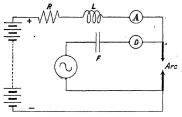
Figure 1: Diagram of the circuit built by Duddell to drive the electric arc with an oscillating circuit [14].

During his investigations, Duddell obtained other interesting results. He also built an oscillating circuit with an electrical arc and a constant source [15]:

“… if I connect between the electrodes of a direct current arc […] a condenser and a self-induction connected in series, I obtain in this shunt circuit an alternating current. I called this phenomenon the musical arc. The frequency of the alternating current obtained in this shunt circuit depends on the value of the self-induction and the capacity of the condenser, and may practically be calculated by Kelvin’s well-known formula [16].”

The block diagram of this circuit is shown in Fig. 2.

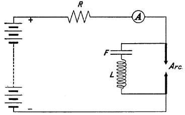
Figure 2: Diagram of the circuit with a constant source of current built by Duddell to obtain a musical arc [14].

Duddel well identified that it is

“the arc itself which is acting as a converter and transforming a part of the direct current into an alternating, the frequency of which can be varied between very wide limits by alterning the self-induction and capacity.”

To observe this effect, Duddell showed that the change in the potentiel $\delta V$ and in the corresponding current $\delta A$ between the ends of the arc must obey to $-\frac{\delta V}{\delta A}\geq r$ where $r$ is the resistance of the capacitor circuit. This means that the arc can be seen as presenting a negative resistance (a concept introduced by Luggin [17]). The various behaviors obtained by Duddell were as follows.

• When the arc is supplied with an oscillating current, he obtained humming which are nearly periodic (Fig. 3a) and hissing which are very irregular and whose frequence is such as $f_{\rm hissing}\approx 100f_{\rm humming}$ (Fig. 3b).

• When the arc is supplied with a constant current, he obtained a self-oscillating electrical arc, a regime he called intermittent or musical.

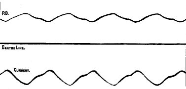
(a) Humming: $\overline{U}=50.5$ V, $\overline{I}=15.2$ A

Top curve = potential difference (PD)

Bottom curve = current

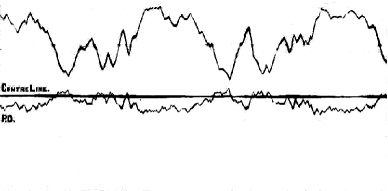
(b) Hissing: $\overline{U}=38$ V, $\overline{I}=22.3$ A

Top curve = current

Bottom curve = potential difference (PD)

Figure 3: Two types of oscillating arc supplied with an oscillating current. Centre line = 40 V = 20 A. With the original figure size, 1 mm = 0.5 V = 0.186 A = $\frac{1}{6400}s$. From [14].

Hissing and intermittent regimes clearly correspond to nonlinear oscillations since not obeying Thomson’s formulae for the period of oscillations. Duddell proposed the formula

$$T=\frac{2\pi}{\displaystyle\sqrt{\displaystyle\frac{1}{LC}-\frac{R^{2}}{4L^{2}}}}$$ (1)

for their period [18]. But there is an ambiguity in Duddell’s work since intermittent (non-linear) and musical (linear since obeying to Thomson’s formula) are not distinguished. Duddell quoted André Blondel (1863-1938) for his observation of the hissing and the intermittent arcs [19].

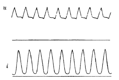
(a) Musical oscillations

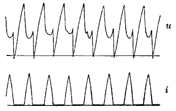
(b) Discontinuous or intermittent oscillations

Figure 4: The two types of oscillations produced by a musical arc and distinguished by Blondel. Musical oscillations are very stable but discontinuous (intermittent) oscillations are only observed when the arc is close to its limit of stability. From [20].

Blondel was assigned to the Lighthouses and Beacons Service, to conduct research on electric arc in order to improve the outdated French electrical system. He made an extensive analysis of the musical arc [20] using Duddell’s circuit (Fig. 2). Blondel, who named it the “singing arc”, clearly distinguished two types of oscillations which were not very well defined in Duddell’s work. The first type corresponds to musical oscillations as used by Duddell to play tunes at a meeting of the Institution of Electrical Engineers using an arrangement of well-chosen capacitors and a keyboard [14]. According to Blondel, these oscillations are nearly sinusoidal (Fig. 4a). The second type corresponds to discontinuous oscillations (Fig. 4b) and were termed “intermittent” by Duddell. In these regimes, already observed in 1892 by Blondel [19] and quoted in [14], the arc can blow out and relight itself with great rapidity. Blondel explained that such intermittent (or discontinuous) regimes are observed when the circuit is placed close to the limit of stability of the arc. Unfortunately, Blondel qualified these second type of oscillations as hissing (“sifflantes” or “stridentes”) although they have nothing o do with the hissing regime observed by Duddell (compare Fig. 3b with Fig. 4b).

Blondel also observed irregular intermittent oscillations as shown in Fig. 5. These periodic oscillations are quite interesting today because they have obviously recurrent properties and could therefore be a good candidate for being considered as chaotic.

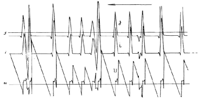
Figure 5: Oscillations “with 3 or 4 alternations” observed with an musical arc between a copper anode and a carbon cathod. From [20].

2.3 From the Audion to the Multivibrator

Although the “audion”, a certain type of triode, was invented in 1907 by Lee de Forest (1873-1961) [25], it was not until the First World War that it was widely distributed for military and commercial purposes. During the summer of 1914, the French engineer Paul Pichon (18??-1929) who deserted the French Army in 1900 and had emigrated to Germany, went to USA on an assignment from his employers, the Telefunken Company of Germany, to gather samples of recent wireless equipments. During his tour he visited the Western Electric Company, and obtained the latest high-vacuum Audion with full information on their use. On his way back to Germany he traveled by the Atlantic liner to Southampton. He arrived in London on August 3, 1914, the very day upon which Germany declared war on France. Considered as a deserter in France and as an alien in Germany, he decided to go to Calais where he was arrested and brought to the French military authorities which were represented by Colonel Gustave Ferrié (1868-1932), the commandant of the French Military Telegraphic Service. Ferrié immediately submitted Pichon’s Audion to eminent physicists including Henri Abraham (1868-1943) who was then sent to Lyon in order to reproduce and improve the device. Less than one year after, the French valve known as the lamp T.M. (Military Telegraphy) was born (Fig. 7). After many tests it became evident that the French valve was vastly superior in every way to the soft-vacuum Round valves and earlier Audions.

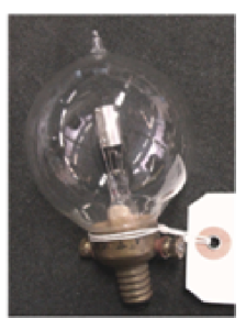
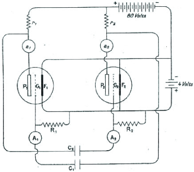
Figure 6: Picture of the original lamp T.M. made by Abraham (1915).

(a) Circuit diagram of multivibrator.

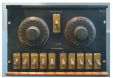
(b) Picture of the original multivibrator.

Figure 7: Circuit diagrams and picture of the multivibrator.

On May 1915, Ferrié asked to Abraham to come back at the École Normale Supérieure (Paris) where, with his colleague Eugène Bloch (1878-1944), he invented the “multivibrator” during the first World War. A multivibrator is a circuit (Fig. 7) made of two lamps T.M. producing sustained oscillations with many harmonics.

Made of two resistors ($R_{1}$ and $R_{2}$) and two capacitors ($C_{1}$ and $C_{2}$), Abraham and Bloch [26, p. 256] explained that reversal of current intensities in plates $P_{1}$ and $P_{2}$ were observed (Fig. 8). They described these oscillations as “a serie of very sudden reversals in currents splitted by long intervals during which variation of the current intensity is very slow” [26]. Two reversals were separated by time intervals corresponding to durations of charge and discharge of capacitors $C_{1}$ and $C_{2}$ through resistors $R_{1}$ and $R_{2}$, respectively. “The period of the system was thus about $C_{1}R_{1}+C_{2}R_{2}$.” The period of these oscillations is therefore associated with some capacitor discharge.

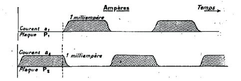
Figure 8: Reversals of the current in plate P₁ and P₂ currents. From [26, p. 256].

3 Differential equations for self-oscillating systems

3.1 Poincaré’s equation for the musical arc

In 1880’s, Poincaré developed his mathematical theory for differential equations and introduced the concept of limit cycle [21] as

“closed curves which satisfy our differential equations and which are asymptotically approached by other curves defined by the same equation but without reaching them.”

Aleksandr Andronov (1901-1952) was commonly credited for the first evidence of a limit cycle in an applied problem, namely in self-sustained oscillating electrical circuit [23]. Nevertheless, it was recently found by one of us [24] that Poincaré gave a series of lectures at the École Supérieure des Postes et Télégraphes (today Sup’Télécom) in which he established that the existence of sustained oscillations in a musical arc corresponds to a limit cycle [22].

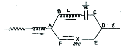
Figure 9: Block diagram of the circuit corresponding to the musical arc as investigated by Poincaré in 1908 [22, p. 390].

Investigating Duddell’s circuit (Fig. 9 which is equivalent to Fig. 2), Poincaré wrote the corresponding differential equations. Designating the capacitor charge by $x$, the current in branch ABCD was thus $x^{\prime}=\frac{dx}{dt}$. Applying Kirchhoff’s law, Poincaré obtained the second-order nonlinear differential equation [22]

$$Lx^{\prime\prime}+\rho x^{\prime}+\theta\left(x^{\prime}\right)+Hx=0\,.$$ (2)

This equation has a general form since the circuit characteristic $\theta\left(x^{\prime}\right)$ describing how the electromotive force depends on the current was not explicitly defined. $\rho x^{\prime}$ corresponds to the internal resistance of the inductor and to the other possible causes of damping, including the radiation from the antenna. $\theta(x^{\prime})$ is the term due to the arc and $\frac{1}{H}$ defines the capacitor. Using the coordinate transformation

$$x^{\prime}=\frac{dx}{dt}=y\,,\,dt=\frac{dx}{dy}=y\,,\,x^{\prime\prime}=\frac{dy}{dt}=\frac{ydy}{dx}\,,$$ (3)

introduced in [21, p. 168], Poincaré obtained

$$Ly\frac{dy}{dx}+\rho y+\theta\left(y\right)+Hx=0\,.$$ (4)

He then stated that

“One can construct curves satisfying this differential equation, provided that function $\theta$ is known. Sustained oscillations correspond to closed curves, if there exist any. But every closed curve is not appropriate, it must fulfill certain conditions of stability that we will investigate.”

Once the direction of rotation defined, Poincaré stated the stability condition [22, p. 391]:

“Let us consider another non-closed curve satisfying the differential equation, it will be a kind of spiral curve indefinitely approaching the closed curve. If the closed curve represents a stable regime, by describing the spiral in the direction of the arrow, one should be brought to the closed curve, and this is the condition according to which the closed curve will represent a stable regime of sustained waves and will provide a solution to this problem.”

The stability condition obviously matches with the definition of a limit cycle. In order to define under which condition a closed curve is stable, Poincaré multiplied Eq. (4) by $x^{\prime}{\rm d}t$ and then integrated the obtained relation over one period of oscillation. Using the fact that the first and the fourth term vanish since corresponding to the conservative component of his nonlinear equation, the obtained condition reduces to

$$\rho\int{{x}^{\prime 2}dt}+\int{\theta\left({{x}^{\prime}}\right){x}^{\prime}dt}=0\,.$$ (5)

Since the first term is quadratic, the second one must be negative. Poincaré then stated that the oscillating regime is stable if and only if function $\theta$ is such as

$$\int{\theta\left({{x}^{\prime}}\right){x}^{\prime}dt}<0\,.$$ (6)

Poincaré thus provided a condition the characteristic $\theta(x^{\prime})$ of the circuit must fulfill to guaranty the presence of a limit cycle in a musical arc. Using the Green formula, this condition was proved [24] to be equivalent to the condition obtained by Andronov [23] more than twenty years later. It is therefore relevant to realize that Poincaré was in fact the first to show that his “mathematical” limit cycle was of importance for radio-engineering. Up to now Andronov was therefore erroneoulsy credited for such insight with a more general equation in his 1929.

3.2 Janet’s equation for series dynamo machine

In April 1919, Janet exhibited an analogy between three electro-mechanical devices, namely i) the series dynamo machine, ii) the musical arc and iii) the triode. For the series dynamo machine, Janet quoted Aimé Witz (1848-1926) [28] who was presenting the experiment as widely known. He only quoted Gérard-Lescuyer in his introduction to Cartan and Cartan’s paper [27]. Janet [12, p. 764] wrote about the series dynamo machine:

“It seemed interesting to me to report unexpected analogies between this experiment and the sustained oscillations so widely used today in wireless telegraphy, for instance, those produced by Duddell’s arc or by the three-electrodes lamps used as oscillators. The production and the maintenance of oscillations in all these systems mainly result from the presence, in the oscillating circuit, of something analogous to a negative resistance.”

He then explained that function $e=f(i)$, where $e$ is the potential difference and $i$ the current, should be nonlinear and should act as a negative resistance. He thus established that these three devices produced non-sinusoidal oscillations and could be described by a unique nonlinear differential equation reading as [12, p. 765]

$$L\frac{d^{2}i}{dt^{2}}+\left[{R-{f}^{\prime}\left(i\right)}\right]\frac{di}{dt}+\frac{k^{2}}{K}i=0$$ (7)

where $R$ corresponds to the resistance of the series dynamo machine, $L$ is the self-induction of the circuit and $K/k^{2}$ is analogous to a capacitor.

Replacing $i$ with $x$, $R$ with $\rho$, $f^{\prime}(i)$ with $\theta(x)$, and $\frac{k^{2}}{K}$ with $H$, this equation becomes Poincaré’s equation (2). As in Poincaré’s work, Janet did not provide an explicit form for nonlinear function $f(i)$. Nevertheless, he wrote the oscillating period as being $T=\frac{2\pi}{k}\sqrt{KL}$, which is equivalent to $T=2\pi\sqrt{CL}$ as obtained by Duddell when resistance $R$ is neglected.

Duddell was quoted by Janet without reference. Janet spoke about Duddell’s arc as a very well-known experiment. Being an engineer in electro-technique, Janet was a reader of L’Éclairage Électrique in which he published more than 20 papers. Consequently, he may have read Poincaré’s conferences…

3.3 Blondel’s equation for the triode

The “triode” equations was proposed six months later by Blondel who used a circuit with an Audion. To achieve this, he proposed to approximate the characteristic as a series of odd terms [29, p. 946]

$$i=b_{1}\left(u+k\nu\right)-b_{3}\left(u+k\nu\right)^{3}-b_{5}\left(u+k\nu\right)^{5}...$$ (8)

From the circuit diagram he used (Fig. 10a) and applying Kirchhoff’s law, he got

$$\begin{array}[]{rl}\displaystyle\frac{{\rm d}^{3}u}{{\rm d}t^{3}}+\frac{r_{2}}{L}\frac{{\rm d}^{2}u}{{\rm d}t^{2}}+\left(\frac{1}{CL}-\frac{r_{1}r_{2}}{L^{2}}\right)\frac{{\rm d}u}{{\rm d}t}&\\[8.5359pt] \displaystyle-\frac{r_{1}}{CL^{2}}u-r_{2}\frac{{\rm d}^{3}i}{{\rm d}t^{3}}-\frac{1}{C}\frac{{\rm d}^{2}i}{{\rm d}t^{2}}&=0\end{array}$$ (9)

By substituting $i$ by its expression in Eq. (9), neglecting the internal resistors and integrating once with respect to time, he thus obtained

$$C\frac{{\rm d}^{2}u}{{\rm d}t^{2}}-\left(b_{1}h-3b_{3}h^{3}u^{2}-...\right)\frac{{\rm d}u}{{\rm d}t}+\frac{u}{L}=0\,,$$ (10)

that is, an equation equivalent to those obtained by Poincaré and Janet, respectively, but where the characteristic was explicitely written. Blondel considered this equation as an approximation.

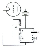
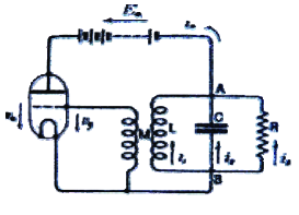
(a) From Blondel [29]	(b) From Van der Pol [30]

Figure 10: Circuit diagrams for the triode oscillator as investigated by Blondel (a) and van der Pol (b). Resistance $r_{2}$ in Blondel’s circuit does not appear in van der Pol’s circuit where resistance $R$ was added in parallel to capacitor $C$.

3.4 The van der Pol equation

One year after Blondel’s paper, van der Pol [30] proposed an equation for a triode oscillator. Its circuit diagram (Fig. 10b) differs from Blondel’s one by the internal resistance he neglected and a resistance $R$ he added in parallel to the capacitor. Van der Pol used a Taylor-McLaurin series expansion to express the characteristic of the triode by the cubic function [30, p. 703]

$$i=\psi\left(kv\right)=\alpha v+\beta v^{2}+\gamma v^{3}\,.$$ (11)

He then obtained the differential equation

$$C\frac{{\rm d}^{2}v}{{\rm d}t^{2}}+\left(\frac{1}{R}-\alpha\right)\frac{{\rm d}v}{{\rm d}t}+\beta\frac{{\rm d}\nu^{2}}{{\rm d}t}+\gamma\frac{{\rm d}\nu^{3}}{{\rm d}t}=0$$ (12)

Van der Pol [30, p. 704] precised that, by symmetry consideration, one can choose $\beta=0$. However, to allow comparison with Blondel’s equation (10), one should also remove the resistance $R$. With Appleton, van der Pol then reduced Eq. (12) [31] to

$$\frac{{\rm d}^{2}v}{{\rm d}t^{2}}+\frac{{\rm d}}{{\rm d}t}\left(\displaystyle\frac{Rv}{L}+\frac{\Psi(v)}{C}\right)+\omega_{0}^{2}v=0$$ (13)

where

$$\Psi(v)=\alpha v+\beta v^{2}+\gamma v^{3}+\delta v^{4}+\epsilon v^{5}+...$$ (14)

They also provided a stability criterion for periodic solutions when coefficients $\alpha$, $\beta$, $\gamma$, etc. are sufficiently small. Solutions to Eq. (13) were then investigated by Appleton and Greaves (see for instance [32, 33]). This is only in 1926 that van der Pol introduced the dimensionless equation [34, 35]

$$\ddot{v}-\epsilon(1-v^{2})\dot{v}+v=0\,.$$ (15)

This equation quicly became popular in radio-electricity. It can be found in a book review (1935) by Robert Mesmy [36] associated with van der Pol’s name and the relaxation oscillations. In [37, p. 373], this equation was mentioned as follows.

“As a typical example of the technique of isoclines, one can use the study of an equation proposed by van der Pol in the phase plane which, we already know it, is called the van der Pol equation”

Quoting [37], Minorsky [39] used the same name. If the van der Pol equation is only an example among many others in Ref. [37], its role is far more important in [39]. Van der Pol’s breakthrough was to propose a dimensionless equation which can thus be used to explain various systems regardless their origins. From that point of view, van der Pol was the first to write a propotypal equation. In doing that, he assimilated the fact that the dynamical nature of the behaviours observed was much more important than a physical explanation as provided, for instance, by Blondel [20, 29]. Van der Pol is therefore correctly credited for this equation written in its simplest form in 1926. Van der Pol also pushed the analysis further by investigating some solutions to his equation.

3.5 Some equations for the multivibrator

In his 1926 paper [3], van der Pol proposed an equation for the multivibrator based on current and potential departures from the unstable equilibrium values. Surprisingly, he had to take into account “the inductance $L$ of the wires connected to the two capacities” but neglected, “for simplicity, the influence of the anode potential on the anode current.” Assuming that the triodes are exactly equal, van der Pol showed that the prototypical equation (15) “represents the action of the multivibrator”. Consequently, “the special vibration of the multivibrator represents an example of a general type of relaxation-oscillations”.

Without taking into account the inductance of the wires, Andronov and Witt obtained another set of equations [38]

$$\left\{\begin{array}[]{l}\displaystyle\dot{x}=\frac{ax-y\varphi^{\prime}(y)}{\phi^{\prime}(x)\varphi^{\prime}(y)-a^{2}}\\[8.5359pt] \displaystyle\dot{y}=\frac{ay-x\varphi^{\prime}(x)}{\phi^{\prime}(x)\varphi^{\prime}(y)-a^{2}}\end{array}\right.$$ (16)

where $x=Ri$, $y=Ri$, and $a=\frac{r+R}{Rr}$ (Fig. 11). The characteristic $I_{k}=\varphi(Ri_{k})$ ($k=1,2$) were approximated by $\varphi(\xi)=\frac{1}{1+\xi^{2}}$. Andronov and Witt performed a dynamical analysis of their system of equations for the multivibrator.

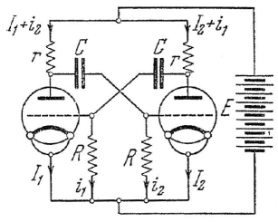
Figure 11: Block diagram of the multivibrator considered by Andronov and Witt (from [38]).

They found that system (16) has three singular points, one located at the origin of the phase space is a saddle and, two symmetry-related singular points defined by

$$x=y=\pm\sqrt{\displaystyle\frac{1-a}{a}}$$ (17)

are unstable (the type is not given with more precision). They then described a typical trajectory (Fig. 12) starting from the initial condition $a_{0}$. They observed a transient regime aAbBcCdDeEfF up to a $\omega$-limit set, made of $\omega\Omega\sigma\Sigma$, which is a limit cycle. They mentioned a “discontinuous curve” for which the jumps occur between $\omega$ and $\Omega$ and, $\sigma$ and $\Sigma$. This trajectory has the very characteristics of “relaxation oscillations” but was not designated by such a name.

Figure 12: The trajectory solution to system (16) investigated by Andronov and Witt (from [38]).

4 Birth of relaxation oscillations

Once the equation written, the job is just beginning. It remains to investigate the corresponding solutions. In 1925, van der Pol distinguished a “separate group” of oscillations whose period can no longer be described by the Thomson’s fomula [16]. Duddell, and then Blondel, already remarked that “the oscillation frequency of the musical arc was variable and not well defined […] In the intermittent case, it has nothing to do with the eigen-frequency of the oscillating circuit” [20]. In 1925, van der Pol remarked [40] that there are some oscillations which

“diverge considerably from the sine curve, being more peaked. Moreover, the frequency is no longer determined by the equation $\omega=\frac{1}{\sqrt{LC}}$ and the time period is approximately the product of a resistance by a capacitor, i.e. a relaxation time. Such oscillations belong to a separate group and are conveniently named “relaxation-oscillations”.”

Van der Pol later noted that “the period of these new oscillations is determined by the duration of a capacitor discharge, which is sometimes named a “relaxation time” [41, p. 370]. Since non-corresponding to the mostly investigated solutions, van der Pol considered his results important enough to publish them at least four times:

1. Over Relaxatietrillingen [42] (in Dutch);

2. Over Relaxatie-trillingen [34] (in Dutch);

3. Über Relaxationsschwingungen [35] (in German);

4. On relaxation-oscillations [3] (in English).

All these contributions have the same title and almost the same content. Consequently, the paper (in Dutch) which was published in 1925 should be quoted as the first paper where relaxation oscillations were introduced. Nevertheless, their conclusions differ in the choice for the devices exemplifying the phenomenon of relaxation oscillations. They were

1. a Wehnelt interrupter (without reference): this example comes from Blondel’s paper [43] (Fig. 13a) but very suggestive relaxation oscillations can also be found in [44] (Fig. 13b);

2. a separate excited motor fed by a constant rotating speed series dynamo and possibly heartbeats;

3. the three previous examples;

4. Abraham and Bloch’s multivibrator,

respectively. Van der Pol was therefore aware of these prior works presenting self-sustained oscillations and whose some of them (Figs. 3b and 4b) were obviously nonlinear since not satisfying the Thomson formula. Van der Pol recognized something special in these dynamics. In order to enlarge the interest for these new dynamical features, he made an explicit connection with electro-chemical systems (the Wehnelt interrupter). He may have not quoted the electric arc because it became an obsolete device since Audion was widely sold. More surprisingly, van der Pol only quoted the well-known multivibrator in his most celebrated paper [3], which is the single one written in English (we recall that not mentionning the first three examples is one of the very few changes compared to his three previous papers). This could be explained by the fact that only the multivibrator was then considered as a “modern” system.

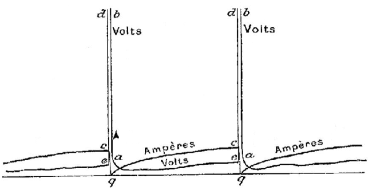
(a) From Blondel [43]

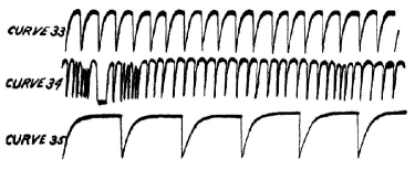
(b) From Compton [44]

Figure 13: Current observed in a Wehnelt interrupter.

The key point is that van der Pol started to investigate solution, not when $\epsilon\ll 1$ as commonly considered, but when $\epsilon\gg 1$. Van der pol distinguished various cases, speaking about the “well-known aperiodic case”, which refers to Pierre Curie’s classification of transient regimes [45]. Note that Eq. (1) in [3] is equivalent to Eq. (2) in Curie’s paper. Moreover, it is possible that van der Pol got the idea to use a prototypical equation from Curie’s paper where the study is performed on a “reduced equation”. This is in fact a dimensionless equation where “each of its terms […] has a null dimension with respect to the fundamental units.” Curie’s paper was known from the electrical engineers since it was quoted by Le Corbeiller in [46] who confirmed that “M. van der Pol [applied] it to the much more complicated case of Eq. (15).” Curie’s paper was also used in [36] without quotation and in [47] with an explicit quotation.

Using a series of isoclynes, that is, of curves connecting all points for which $\frac{{\rm d}v}{{\rm d}t}$ is a given constant, van der Pol draw three cases of oscillation for $\epsilon=0.1$, 1 and 10, respectively. He focussed his attention on the third case (Fig. 14) which was designated as “quasi-aperiodic” because the oscillations quickly converge toward a closed curve, the aperiodicity being only observed during the transient regime. It actually seems that van der Pol erroneously qualified the closed curve itself as an aperiodic behavior. It would be an example of a lack of rigor and, source of contradiction as exemplified in [3, p. 987]: “our equation for the quasi-aperiodic case, which differs considerably from the normal approximately sinusoidal solution, has again a purely periodic solution, …” How can we have a clear understanding of a quasi-aperiodic solution which is purely periodic?

The plot of the periodic solutions of equation (15) was one of the result which was mostly appreciated in van der Pol’s paper. Van der Pol did not realized that this periodic solution was Poincaré’s limit cycle. He did not use this expression before 1930 [48, p. 294]

“We see on each of these three figures a closed integral curve; this is an example of what Henri Poincaré has called a limit cycle [23], because integral curves approach it asymptotically.”

Nevertheless, he quoted the paper in which Elie Cartan (1869-1951) and his son Henri Cartan (1904-2008) established the uniqueness of the periodic solution to Janet’s equation (7) [27].

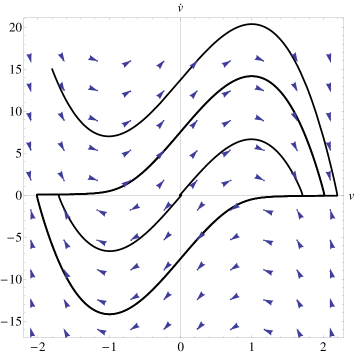
Figure 14: Isoclines in a $\dot{v}$-$v$ plane diagram. The heavy line follow the slopes indicated on the isoclines, thus forming a solution to equation (15). Drawn in the spirit of the original figure.

Van der Pol [3, p. 987] determined graphically the period of relaxation oscillations starting from the time series (Fig. 15). According to this figure, it is obvious that the period for relaxation oscillations (from a maximum to the next maximum) is equal to twenty and not approximatively equal to $\varepsilon=10$ as claimed by van der Pol [3, p. 987]. It is rather surprising that van der Pol did not provide $T=2\epsilon$, particularly because he correctly estimated the period to be $2\pi$ for $\epsilon=0.1$. This lack of rigor was pointed out by Alfred Liénard (1869-1958) in [49, p. 952] where he demonstrated the existence and uniqueness of the periodic solution to a generalized van der Pol equation. Van der Pol had already realized his mistake and provided (in 1927) a better approximation for the period according to the formula [50, p. 114]:

$$T=\left({3-2\log_{e}2}\right)\varepsilon=1.61\varepsilon\,.$$ (18)

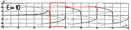
Figure 15: Relaxation oscillations solution to the van der Pol equation for $\epsilon=10$. From [3, p. 986].

For $\epsilon=10$, this leads to $T=16.1$ which is still far away from the measured value of 20. Seventeen years later, Jules Haag (1882-1953) provided a better approximation [51] by using Asymptotic Methods [52, p. 103]:

$$\begin{array}[]{rl}T&=\displaystyle\left[\displaystyle 3-2\log\left(2\right)\right]\varepsilon+\frac{12.89}{\varepsilon^{1/3}}\\[8.5359pt] &\displaystyle~{}~{}~{}+\frac{2}{\varepsilon}\left[{-3.31+\frac{19}{9}\log\left(\varepsilon\right)}\right]-\frac{4}{\varepsilon^{5/3}}+\cdots\end{array}$$ (19)

Then, replacing $\varepsilon$ by ten into Eq. (19) one finds a value (20.3) closer to twenty,.

5 Turning relaxation oscillations as a concept

5.1 Some insights on the German school

German scientists were not quoted up to now. We will focus our attention on a few contributions. Of course, sustained oscillations were found in a symmetrical pendulum by Georg Duffing [55]. Sustained oscillations were found in a thermionic system by Heinrich Barkhausen (1881-1956) and Karl Kurz [56]. It seems that this contribution triggered the interest of German physicists for sustained oscillations in electro-technical or electronic devices. An important contribution was provided by Erich Friedländer in 1926, a few months before van der Pol’s papers were published. Note that Friedländer is quite often quoted in [37]. Entitled “On relaxation oscillations (Kippschwingungen) in electronic vacuum tubes”, Friedländer started his paper as follows [57].

“it has been already pointed out that several systems can produce self-excited oscillations which do not obey to the Thomson formula. […] The best control devices which are enable to enforce such an energy oscillating exchange are now arc, neon lamp, vacuum tube.”

Friedländer then evidenced an oscillating regime in a glow discharge (Fig. 16).

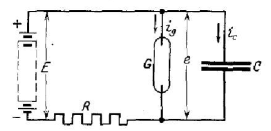
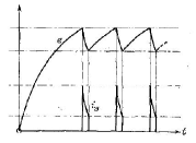
(a) Block diagram	(b) Nonlinear oscillations

Figure 16: Oscillations in a glow discharge circuit. From [57].

Friedländer then explained how an alternating potential (Fig. 17b) occurs in a circuit with an arc lamp (Fig. 17a). With such a circuit, he obtained some intermittent regimes as shown in Fig. 17c, and which correspond to Duddell’s intermittent regime or Blondel’s discontinuous arc.

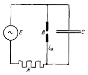
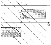
(a) Block diagram	(b) Circulation diagram
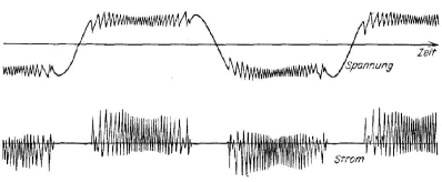
(c) Intermittent oscillations

Figure 17: Oscillations in a glow discharge circuit. From [57].

Friedländer also investigated a triode circuit (Fig. 18a) where he observed relaxation oscillations (Fig. 18b) when the grid current did not reach saturation. He then investigated stability conditions for some particular regimes in a second paper [58].

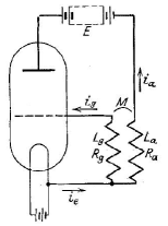
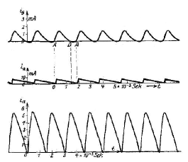
(a) Block diagram	(b) Relaxation oscillations

Figure 18: Sustained oscillations in a circuit with a triode. From [57].

Few years later Erich Hudec developed a theorie for “Kippschwingungen” in a triode circuit with a cubic characteristic (Fig. 19), and presenting various relaxation oscillations [59]. Hudec quoted Friedländer but not van der Pol. Friedrich Kirschstein presented many relaxation oscillations observed in various electronic circuits [60]. Contrary to Hudec, he prefered the word “Relaxationsschwingungen” to “Kippschwingungen”, and quoted van der Pol [35]. With the graphical method used by van der Pol (Fig. 14), he was looking for stable sustained solution (Fig. 20), but as in van der Pol’s work, no link was made with Poincaré’s limit cycle. To end this brief review, W. Pupp did a similar contribution one year before Kirschstein, showing stable sustained oscillations — in a plane projection — produced by an impulse radio emitter [61].

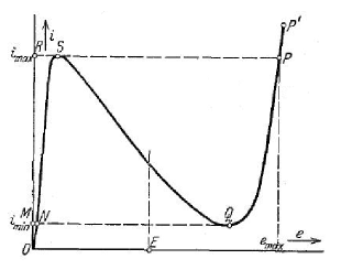
Figure 19: Cubic characteristic of the triode circuit investigated by Hudec [59].

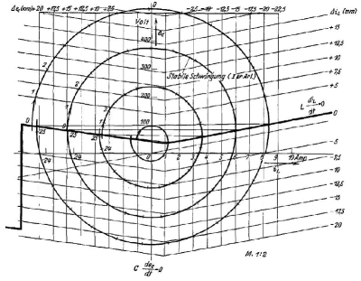
Figure 20: Plane diagram for representing solution to the triode circuit as investigated by Kirschstein [60].

5.2 Van der Pol’s lectures in France

In 1926, van der Pol described the relaxation-oscillations as follows [3].

“It is seen that the amplitude alters very slowly from the value 2 to the value 1 and then very suddenly it drops to the value -2. Next we observe a very gradual increase from the value -2 to the value -1 and again a sudden jump to the value 2. This cycle term proceeds indefinitely.”

As van der Pol later precised [41]

“their form […] is characterized by discontinuous jumps arising each time the system becomes unstable, that is, periodically [and] their period is determined by a relaxation time.”

He also remarked that these oscillations are easily synchronized with a periodic external forcing term [53]. In 1931, Le Corbeiller described them as “oscillations whose shape is very different and whose prototype is provided by a slow charge of a capacitor, followed by its rapid discharge, the cycle being indefinitely repeated” [54].

As we showed the French school of electrical engineers and/or mathematicians contributed quite a lot to the early developments of a theory in non-linear oscillations. As briefly mentionned in the previous section, German school was active too, but it was a little bit isolated, probably due to the particular political context during this period. Its actual contribution remains to be more extensively investigated. In anyway, it is not surprising that van der Pol, deeply involved in this area of research, was regularly invited in France to present his works on relaxation oscillations. During each of his lectures he exhibited the differential equation (15). Then, van der Pol [41, p. 371] provided a non-exhaustive list of examples:

“Hence with Aeolian harp, as with the wind blowing against telegraph wires, causing a whistling sound, the time period of the sound heard is determined by a diffusion-or relaxation time and has nothing to do with the natural period of the string when oscillating in a sinusoidal way. Many other instances of relaxation oscillations can be cited, such as: a pneumatic hammer, the scratching noise of a knife on a plate, the waving of a flag in the wind, the humming noise sometimes made by a watertap, the squeaking of a door, a steam engine with much too small flywheel, […], the periodic reoccurence of epidemics and economical crises, the periodic density of an even number of species of animals, living together and the one species serving as food to the other, the sleeping of flowers, the periodic reoccurence of showers behind a depression, the shivering from cold, the menstruation and finally the beating of the heart.”

Starting from these examples, van der Pol wanted to show that relaxation oscillations are ubiquitous in nature. All of them, although apparently very different, belong in fact to the new class of relaxation oscillations he discovered as solutions to “his” prototypical equation (15).

With such an attitude, van der Pol tried to generalize the notion of relaxation oscillations in order to confer it the value of a concept. This attempt for a generalization was received with a mixed feeling in France. On the one hand, a certain scepticism on behalf of the French and international scientific community like that expressed by Liénard [49, p. 952] who noted that the period of relaxation oscillations van der Pol graphically deduced [3] was wrong or Rocard [62, p. 402] which was speaking of a “very extended generalization of the concept of relaxation oscillations”. The French school was complaining about a certain lack of rigor in van der Pol’s works. In U.S.S.R., Leonid Mandel’shtam [63] and his students Andronov, Khaikin & Witt [37] did not make use of the terminology “relaxation oscillations” introduced by van der Pol. They prefered the term “discontinuous motions”, as used by Blondel, particularly because it suggests a description of these oscillations in terms of slow/fast regimes. This approach only became mature in the context of the singular perturbation theory whose according to O’Malley [64], early motivations arose from Poincaré’s works in celestial mechanics [65], works by Ludwig Prandtl (1875-1953) in fluid mechanics [66] and van der Pol’s contribution.

On the other hand, an extreme focusing on relaxation oscillations took the shape of a “hunting of the relaxation effect”. Minorsky spent the fourth part of his book [39] on relaxation oscillations, quoting various examples as suggested in Le Corbeiller’s book [67]. In France, the neurophysiologist Alfred Fessard (1900-1982) exhibited relaxation oscillations in nervous rhythms (Fig. 21) [68], the engineer in hydrodynamics François-Joseph Bourrières (1880-1970) found some of them in a hose through which a fluid was flowing [69]. Concerning the list of typical examples proposed by van der Pol [41, p. 371] some of them could be considered as being non justified. But van der Pol [70] showed quite convincing time series (Fig. 22a) produced by a heart model made of three relaxation systems (Fig. 22b). Some periodic reoccurence of economical crisis were studied at that time by the Dutch economist Ludwig Hamburger [71]. He explained that sales curves correspond in many aspects to relaxation oscillations (Fig. 23).

(a) Global electromyogram of a strong voluntary contraction by a men.

(b) Pulsation of a nervous ending observed using the local action potential.

Figure 21: Two physiological examples where relaxation oscillations were found by Fessard [68].

(a) Heartbeats

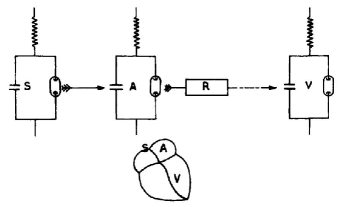
(b) The heart model as three three relaxation systems

Figure 22: Heartbeats produced by a heart model made of three relaxation systems. S $\equiv$ sinus, A $\equiv$ auriculum and V $\equiv$ ventriculum. R is a delay system for reproducing the time necessary for a stimulus to be transmitted through the auriculo-ventricular bundle. From [70].

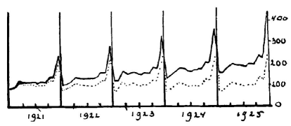
Figure 23: Ratios of monthly sales in shop “Five-and-ten chain stores” in USA between 1921 and 1925. The solid line corresponds to the real data, the dotted curve to what occurs after eliminating the annual growth. From Hamburger [71].

Sleep of flowers was also seriously investigated by Antonia Kleinhoonte in her thesis [72]. The leaf movement of jack-bean, Canavalia ensiformis, plants daily fluctuates as relaxation oscillations. Kleinhoonte’s work is considered as a confirmation of a circadian rhythm in plants, as proposed by Jagadish Chandra Bose [73]. The time series shown in Fig. 24 was included in one of van der Pol’s paper [48, p. 312]. Nonlinear oscillations were already observed in the Lotka-Volterra model [74, 75]; although this model was conservative, the obtained oscillations were nonlinear and do not look too different from the relaxation oscillations observed in dissipative systems.

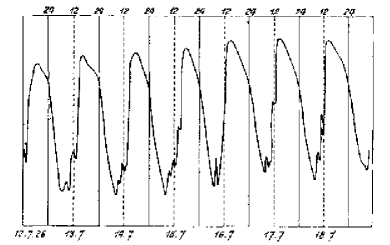
Figure 24: Leaf movement of Canavalia ensiformis plants revealing a circadian rhythm and considered as a relaxation oscillation by van der Pol. From Kleinhoonte [72].

5.3 Le Corbeiller’s contribution

In the early 1930s, the French engineer Philippe Le Corbeiller (1891-1930), who was assisting van der Pol during his lectures in France, contributed to popularize the concept of relaxation oscillations. After the First World War, he became an expert in electronics, acoustics and worked for the French Ministry of Communication. In his lectures, he most often promoted van der Pol’s contribution [67, p. 4] as for instance follows.

“ […] this is a Dutch physicist, M. Balth. van der Pol, who, by his theory on relaxation oscillations (1926) made decisive advances. Scholars from various countries are working today to expand the path he traced; among these contributions, the most important seems to be that of M. Liénard (1928). Very interesting mathematical research are pursued by M. Andronow from Moscow.”

Poincaré was mentioned for the limit cycle that Andronov identified in 1929 [23]. Blondel was quoted for having suggested the term of “variance” for negative resistance, Janet for his popularization of the Gérard-Lescuyer experiments, but Duddell was forgotten. With such a presentation, van der Pol was presented as the main contributor who triggered the interesting approach (before was the “old” science, after was the “modern” science). This is in fact only based on the word “relaxation”. When he spoke about preceding works, only the experimental evidences supporting van der Pol’s relaxation theory were mentionned. In his conclusion, Le Corbeiller [67, p. 45] seems to come back to a more realistic point of view:

“The mathematical theory of relaxation oscillations only begun, several phenomena of which we spoke are just empirically known and, therefore, can surprise us […]. In a word, we have in the front of us the immense field of nonlinear systems, in which we have only begun to penetrate. I would hope that these conferences have shown all the interest we can have in its exploration.”

But the story was already written: Balthazar van der Pol was the first one to give a “general framework” to investigate all these behaviors. He was thus promoted as the heroe of this field. To be complete about Le Corbeiller’s position, let us mention that he became close enough to van der Pol’s widow Pietronetta Posthuma (1893-1984) to marry her in New York, on May 7, 1964.

6 Conclusion

We showed that many self-sustained oscillating experiments were observed before the 1920s, some of them being well investigated, experimentally as well as theoretically. Blondel should be mentionned as being the one who pushed quite far explainations for the physical mechanisms underlying such phenomena. The key property of these new oscillations was that they were not linear, that is, not associated with a frequency matching with the eigen-frequency of the circuit (Thomson’s formula). Blondel noted such a property. Van der Pol then distinguished a particular type of oscillations which greatly differ from sinusoidal oscilaltions and whose period does not match with the Thomson formula. He proposed a generic name, the “relaxation oscillations”, but no clear mathematical definition was proposed. A “slow evolution followed by a sudden jump” is not enough to avoid ambiguous interpretation. As a consequence, many “relaxation oscillations” were seen in various contexts. If we consider that relaxation is justified by a kind of “discharge property” by analogy with a capacitor, some of the examples provided by van der Pol, clearly not belong to this class of oscillations, as well exemplified by the plant leaf movement.

The so-called van der Pol equation — in its interesting simplified form — was written for the first time by van der Pol. This equation was not the first one where self-oscillating behaviours were observed but this is the first “reduced equation” in Curie’s sense. The preceding equations were obtained for some particular experimental set-up as exemplified by Poincaré, Blondel and Janet. Van der Pol spent a large amount of energy to convince people that his simple equation and its solutions could serve as a paradigm to explain various behaviors: the breakthrough was also that what is important is the dynamics and no longer the physical processes. With its graphical representation, he also contributed to change the way in which these nonlinear phenomena had to be investigated. To that respect, associating his name with this simple equation is one of the possibilities to thank him.

7 Remark

This article has been entirely copied by C. Letellier in the chapter 2 pp. 101-137 of his book entitled Chaos in Nature but in omitting the reference to the present work which was directly issued from the original research made by Ginoux [10] in his second PhD-thesis in History of Sciences.

References

- [1] F. L. H. H. Stumpers, Balth. van der Pol’s work on nonlinear circuits, IRE Transactions on Circuit Theory, 7 (4), 366-367, 1960.
- [2] M.-L. Cartwright, Balthazar van der Pol, Journal of the London Mathematical Society, 35, 367-376, 1960.
- [3] B. van der Pol, On “relaxation-oscillations”, The London, Edinburgh, and Dublin Philosophical Magazine and Journal of Science, 7 (2), 978-992 (1926).
- [4] M.-L. Cartwright & J. E. Littlewood, On non-linear differential equations of the second order: I. The equation , large, Journal of the London Mathematical Society, 20, 180-189, 1945.
- [5] G. Israel, Technological innovations and new mathematics: van der Pol and the birth of non-linear dynamics, Technological concepts and mathematical models in the evolution of modern engineering systems, (M. Lucertini, A. M. Gasca & F. Nicolo, Ed.), Birkhäuser (Basel), pp. 52-78 (2004).
- [6] D. Aubin & A. Dahan, Writing the history of dynamical systems and chaos: Longue durée and revolution, disciplines and cultures, Historia Mathematica, 29, 273-339 (2002).
- [7] A. Dahan Dalmedico, Early developments of nonlinear science in soviet Russia: The Andronov school at Gor’kiy (in collaboration with Irina Gouzévitch), Science in Context, 17, 235-265 (2004).
- [8] S. Diner, Les voies du chaos déterministe dans l’école russe, in Chaos et déterminisme, (A. Dahan-Dalmedico, J.-L. Chabert, & K. Chemla, Ed.), Seuil (Paris), pp. 331-368 (1992).
- [9] R. Merton, The Matthew effect in science, Science, 159, 56-63 (1968).
- [10] J. M. Ginoux, Analyse mathématique des phénomènes oscillatoires non linéaires, Ph’D Thesis, Université of Paris vi (2011).
- [11] J. M. A. Gérard-Lescuyer, On an electrodynamical paradox, Philosophical Magazine, v, 10, 215-216 (1880).
- [12] P. Janet, Sur une analogie électro-technique des oscillations entretenues, Comptes-Rendus de l’Académie des Sciences, 168, 764-766 (1919).
- [13] P. Janet, Note sur une ancienne expérience d’électricité appliquée, Annales des P.T.T., 14, 1193-1195 (1925).
- [14] W. Duddell, On rapid variations in the current through the direct-current arc, Journal of the Institution of Electrical Engineers, 30 (148), 232-267 (1900).
- [15] W. Duddell, The arc and the spark in Radio-Telegraphy, Science, 26, 815-824 (1907).
- [16] W. Thomson, On transient electric currents, Philosophical Magazine, iv, 5, 393-405, (1853).
- [17] H. Luggin, Versuche und Bemerkungen über den galvanischen Lichtbogen, Centralblatt für Elektrotechnik, 10, 567-581 (1888).
- [18] W. Duddell, The musical arc, The Electrician, 52, 902, (1901).
- [19] A. Blondel, Etudes expérimentale sur l’arc à courants alternatifs, La Lumière électrique, 43 (2), 51-61 (1892).
- [20] A. Blondel, Sur les phénomènes de l’arc chantant, Éclairage Électrique, 44 (28), 41-58 and 81-104 (1905).
- [21] H. Poincaré, Sur les courbes définies par une équation différentielle, Journal de Mathématiques Pures et Appliquées, iv, 2, 151-217 (1886).
- [22] H. Poincaré, Sur la télégraphie sans fil, Lumière électrique, 4, 259-266, 291-297, 323-327, 355-359 & 387-393 (1908).
- [23] A. A. Andronov, Les cycles limites de Poincaré et la théorie des oscillations auto-entretenues, Comptes-Rendus de l’Académie des Sciences, 189, 559-561 (1929).
- [24] J.M. Ginoux & L. Petitgirard, Poincaré’s forgotten conferences on wireless telegraphy, International Journal of Bifurcation & Chaos, 11 (20), 3617-3626, (2010).
- [25] L. de Forest, Oscillation-responsive device, US Patent n°836070 (1906) and Wireless telegraphy, US Patent n° 841386 (1907).
- [26] H. Abraham & E. Bloch, Mesure en valeur absolue des périodes des oscillations électriques de haute fréquence, Annales de Physique, 9, 237-302 (1919).
- [27] E. Cartan & H. Cartan, Note sur la génération des oscillations entretenues, Annales des P.T.T., 14, 1196-1207 (1925).
- [28] A. Witz, Des inversions de polarité dans les machines série-dynamos, Comptes-Rendus de l’Académie des Sciences, 108, 1243-1246 (1889).
- [29] A. Blondel, Amplitude du courant oscillant produit par les audions générateurs, Comptes-Rendus de l’Académie des Sciences, 169, 943-948 (1919).
- [30] B. Van der Pol, A theory of the amplitude of free and forced triode vibrations, Radio Review (London), 1, 701-710 and 754-762 (1920).
- [31] E. V. Appleton & B. Van der Pol, On a type of oscillation-hysteresis in a simple triode generator, Philosophical Magazine, vi, 43, 177-193, 1922.
- [32] E. B. Appleton, THe automatic synchronization of triode oscillators, Proceedings of the Cambridge Philosophical Society, 21, 231-248 (1922).
- [33] E. V. Appleton & W. M. H. Greaves, On the solution of the representative differential equation of the triode oscillator, Philosophical Magazine, vi, 45, 401-414 (1923).
- [34] B. Van der Pol, Over ,,Relaxatie-trillingen”, Tijdschrift van het Nederlandsch Radiogenootschap, 3, 25-40 (1926).
- [35] B. Van der Pol, Über ,,Relaxationsschwingungen”, Jahrbuch der drahtlosen Telegraphie und Telephonie, 28, 178-184 (1926).
- [36] R. Mesny, Radio-électricité générale. i Étude des circuits et de la propagation, E. Chiron Ed. (Paris), 1935.
- [37] A. A. Andronov S. E. Khaikin, Theory of oscillations, (in Russian), O.N.T.I, Moscow-Leningrad (1937). It should be understood that this edition differs considerably from the one translated by Lefschetz as well as the later editions highly revised and highly augmented by N. A. Zheleztsov.
- [38] A. A. Andronov A. Witt, Discontinuous periodic motions and the theory of Abraham & Bloch’s multivibrator (in Russian), Bulletin of the Academy of Science of SSSR, 8, 189-192, 1930.
- [39] N. Minorsky, Introduction to non-linear mechanics, Edwards Ed. (Ann Arbor), 1974.
- [40] B. van der Pol, Het onderling verband tusschen eenige moderne vorderingen in de draadlooze telegrafie en telefonie, Polytechnish Weekblad, 19, 791-794, 1925.
- [41] B. Van der Pol & J. Van der Mark, Le battement du cœur considéré comme oscillation de relaxation et un modèle électrique du cœur, L’Onde Électrique, 7, 365-392 (1928).
- [42] B. Van der Pol, Over Relaxatietrillingen, Physica, 6, 154-157 (1926).
- [43] A. Blondel, Sur l’interrupteur électrique Wehnelt, Comptes-Rendus de l’Académie des Sciences, 128, 877-879 (1899).
- [44] K. T. Compton, A study of the Wehnelt electrolytic interrupter, Physical Review, i, 30, 161-179 (1910).
- [45] P. Curie, Équations réduites pour le calcul des mouvements amortis, La Lumière Électrique, xli, 31, 201-209, 1891.
- [46] P. Le Corbeiller, Les systèmes auto-entretenus et les oscillations de relaxation, Hermann (Paris), 1931.
- [47] N. Krylov & B. Bogoliubov, Introduction non-linear mechanics (in Russian), Izd. Akad. Nauk SSSR (1937), translated by S. Lefschetz, Princeton University Press, 1943.
- [48] B. Van der Pol, Oscillations sinusoïdales et de relaxation, Onde Électrique, 9, 245-256 & 293-312 (1930).
- [49] A. Liénard, Étude des oscillations entretenues, Revue générale de l’Electricité, 23, 901-912 & 946-954 (1928).
- [50] B. van der Pol, Über ,,Relaxationsschwingungen II”, Jahrbuch der drahtlosen Telegraphic und Telephonie, 29, 114-118 (1927).
- [51] J. Haag, Étude asymptotique des oscillations de relaxation, Annales de l’École Normale Supérieure, III 60, 35-64, 65-111 and 289 (errata) (1943).
- [52] J. Haag, Exemples concrets d’études asymptotiques d’oscillations de relaxation, Annales de l’École Normale Supérieure, III 61, 73-117 (errata) (1944).
- [53] B. van der Pol & J. van der Mark, Frequency demultiplication, Nature, 120, 363-364, 1927.
- [54] P. Le Corbeiller, Les systèmes auto-entretenus et les oscillations de relaxation, Econometrica, 1 (3), 328-332, 1933.
- [55] G. Duffing, Erzwungene Schwingungen bei veranderlicher Eigenfrequenz und ihre technische Bedeutung, Friedr. Vieweg & Sohn Braunschweig (1918).
- [56] H. Barkausen & K. Kurz, Die kurzesten mit Vakuumrohren herstellbaren Wellen, Physikalische Zeitschrift, 21, 1 (1920).
- [57] E. Friedländer, Über Kippschwingungen, insbesondere bei Elektronenröhren, Archiv fur Elektrotechnik, 16, 273-279 (1926).
- [58] E. Friedländer, Über Kippschwingungen, insbesondere bei Elektronenröhren — II. Teil: Die Vorgänge bei Elektronenröhren, Archiv fur Elektrotechnik, 17 (2), 103-142 (1926).
- [59] E. Hudec, Erzwangene, Kippschwingungen und ihre technischen Anwendungen, Archiv fur Elektrotechnik, 22, 459-506 (1929).
- [60] F. Kirschstein, Über ein Verfahren zur graphischen Behadlung elektrischer Schwingungsvorgänge, Archiv fur Elektrotechnik, 24, 731-762 (1930).
- [61] W. Pupp, Über Funkenerregung kurzer elektrischer Wellen unter 1 m Wellenlänge und einen neuartigen Stoßfunkensender, Annalen der Physik, 394 (7), 865-908 (1929).
- [62] Y. Rocard, Sur certains types nouveaux d’oscillations mécaniques, in Livre jubilaire de M. Brillouin, Gauthier-Villars (Paris), pp. 400-408 (1935).
- [63] L. I. Mandel’shtam, N. D. Papaleksi, A. A. Andronov, S. E. Chaikin and A. A. Witt, Exposé des recherches récentes sur les oscillations non-linéaires (in French), Journal de Physique Technique de l’URSS, 2, 81-134 (1935).
- [64] R. E. O’Malley, Singular perturbation theory for ordinary differential equations, Applied Mathematical Sciences, 89, Springer-Verlag, New-York (1991).
- [65] H. Poincaré, Les Méthodes Nouvelles de la Mécanique Céleste, Gauthier-Vilars, 3 volumes, (1892, 1895 and 1899).
- [66] L. Prandtl, Über Fluüssigkeits bewegung bei kleiner Reibung, Verhndlungen des dritten internationalen Mathematik-Kongresses, Tübner, Leipzig, pp. 484-491 (1905).
- [67] Ph. Le Corbeiller, Les systèmes auto-entretenus et les oscillations de relaxation, Hermann, Paris (1931).
- [68] A. Fessard, Les rythmes nerveux et les oscillations de relaxation, L’Année psychologique, 32 49-117, (1931).
- [69] F.-J. Bourrières, Sur un phénomène d’oscillation auto-entretenue en mécanique des fluides, Publications Scientifiques et Techniques du Ministère de l’air, (E. Blondel La Rougery, Ed.), 147, Gauthier-Villars, Paris (1939).
- [70] B. van der Pol, Biological rhythms considered as relaxation oscillations, Acta Medica Scandinavica, 103 (S108), 76-88 (1940).
- [71] L. Hamburger, Een nieuwe weg voor conjunctuur-onderzoek, een nieuwe richtlijn voor conjunctuur-politiek, De Economist, 79 (1), 1-39 (1930) — Analogie des Fluctuations économiques et des Oscillations de relaxation, Institut de Statistique de l’Université de Paris, Supplément aux Indices du Mouvement des Affaires, 9, 1-35 (1931).
- [72] A. Kleinhoonte, De door het licht geregelde autonome bewegingen der Canavalia bladeren, Arch. Neer. Sci. Exca. Natur. B, iii , 5, 1-110 (1929).
- [73] J. C. Bose, Life movements in plants, Transactions of the Bose Institute, 2, 255-597 (1919).
- [74] A. J. Lotka, Analytical note on certain rhythmic relations in organic systems, Proceedings of the National Academy of Sciences (USA), 6 (7), 410-415 (1920).
- [75] V. Volterra, Variazioni e fluttuazioni del numero di individui in specie, animali cunvirenti, Memorie della R. Accademia dei Lincei S., 6 (2), 31-113 (1926).