Poincaré’s forgotten conferences on wireless telegraphy

Abstract

At the beginning of the twentieth century while Henri Poincaré (1854-1912) was already deeply involved in the developments of wireless telegraphy, he was invited, in 1908, to give a series of lectures at the École Supérieure des Postes et Télégraphes (today Sup’Télecom). In the last part of his presentation he established that the necessary condition for the existence of a stable regime of maintained oscillations in a device of radio engineering completely analogous to the triode: the singing arc, is the presence in the phase plane of stable limit cycle. The aim of this work is to prove that the correspondence highlighted by Andronov between the periodic solution of a non-linear second order differential equation and Poincaré’s concept of limit cycle has been carried out by Poincaré himself, twenty years before in these forgotten conferences of 1908.

Keywords: maintained oscillations, wireless telegraphy, limit cycles, stability, singing arc

1 Introduction

The famous correspondence established by the Russian mathematician Aleksandr Andronov (1901-1952) in a note published in the Comptes Rendus of the French Academy of Sciences in 1929 was until now considered by scientists and historians of science as a key moment in the development of the theory of nonlinear oscillations. One of the first to point out the importance of this result was Leonid Mandel’shtam (1879-1944), the Ph-D advisor of Andronov, during the sixth General Assembly of the Union Radio-Scientifique Internationale (U.R.S.I.):

“The relationship between the work of Poincaré, improved by Birkhoff, and those of Lyapunov, and our physical problem was reported by one of us. Three things should be distinguished here. First the qualitative theory of differential equations developed by Poincaré proved very efficient for qualitative discussion of physical phenomena that occur in systems used by radio engineering. But neither the physician nor a fortiori the engineer can not be satisfied with a qualitative analysis. Another series of works of Poincaré provides a method that enables to analyze our problems quantitatively. Finally the work of Lyapunov can give a mathematical discussion of the questions of stability.” [Mandel’shtam et al., 1935, p. 83]

A few years later, Nicolas Minorsky (1885-1970) wrote in his “Introduction to Non-Linear-Mechanics”:

“Andronow was first to suggest that periodic phenomena in non-linear and non-conservative systems can be described mathematically in terms of limit cycles which thus made it possible to establish a connection between these phenomena and the theory of Poincaré developed for entirely different purposes.” [Minorsky, 1947, p. 63]

Since then, many scientists and historians of science have considered Andronov as the first to have emphasized a connection with Poincaré’s works.

“Henceforth, by using, transposing, or extending Poincaré’s arsenal Andronov would endeavor to develop Mandel’shtam’s program. Also, reaping Lyapounov’s heritage, Andronov focused on the problem of stability. Combining Poincaré’s small-parameter method with Lyapounov’s stability theory, he established a method for finding periodic solutions and studying their stability.”
N                                      [Aubin & Dahan, 2002, p. 286]

As above mentioned, let’s notice that the correspondence of Andronov does not only deal with the analogy between the shape of the periodic solution of a nonlinear second order differential equation and Poincaré’s concept of limit cycle. In fact, the result of Andronov is of much greater importance since it concerns the stability of the limit cycle. In other words, it states that the necessary condition for establishing a stable regime of maintained oscillations in a system (a radio engineering device for example) is the existence, in the phase plane, of a stable limit cycle.

Generally, Andronov’s result is associated with that of Balthazar Van der Pol (1889-1959) who is wrongly credited for having highlighted the existence of a limit cycle in an oscillating circuit comprising a triode. Although the triode was invented in 1907, its use was widespread only after the first World War. But at this time, Poincaré had already died prematurely. So, the question that arises then is the following:

What kind of device has been employed by Poincaré

to observe maintained oscillations?

Before the advent of the triode, a device was commonly used in wireless telegraphy: the singing arc. Completely analogous to the triode the singing arc was used to generate electromagnetic waves (radio waves).

During the last two decades of his life, Poincaré had been involved in many research on the propagation of electromagnetic waves. In 1890, he wrote to Hertz to report a miscalculation in his famous experiments. Three years later, he solved the telegraphists equation [Poincaré, 1893]. The following year he published a book entitled: “Oscillations électriques” [Poincaré, 1894] and in 1899 another one: “La Théorie de Maxwell et les oscillations hertziennes” [Poincaré, 1899]. This book, also published in English and German in 1904 and reprinted in French in 1907, has been considered as a reference. In Chapter XIII, page 79 Poincaré stated that the singing arc and the Hertz spark gap transmitter were also analogous except that oscillations are maintained in the first and damped in the second. Thus, from the early twentieth century until his death Poincaré continued his research on wireless telegraphy and on maintained waves and oscillations [Poincaré, 1901, 1902, 1903, 1904, 1907, 1908, 1909abcde, 1910abc, 1911,1912].

On July $4^{th}$, 1902 he became Professor of Theoretical Electricity at the École Supérieure des Postes et Télégraphes (today Sup’Télecom) in Paris where he taught until 1910. The director of this school, Édouard Estaunié (1862-1942), also asked him to give a series of conferences every two years. In 1908, Poincaré chose as the subject: wireless telegraphy. The text of his lectures was first published weekly in the journal La Lumière électrique [Poincaré, 1908] before being edited as a book [Poincaré, 1909d].

In the fifth and last part of these lectures entitled: “Télégraphie dirigée : oscillations entretenues” Poincaré stated a necessary condition for the establishment of a stable regime of maintained oscillations in the singing arc. More precisely, he demonstrated the existence, in the phase plane, of a stable limit cycle.

This paper is organized as follows. In the second section the fifth part of the Poincaré’s conferences [Poincaré, 1908] will be fully presented and analyzed. Then, it will be compared to Andronov’s work of 1929 [Andronov, 1929] presented in the third section and it will be shown in fourth section that Poincaré and Andronov results are completely identical. Thus, the reasons why this fundamental paper of Poincaré has remained in oblivion, for scientists and historians of science for more than one century, will be discussed in the last section.

2 Poincaré’s forgotten conferences on wireless telegraphy

At the end of the nineteenth a device, ancestor of the incandescent lamp, called electric arc was used for illumination of lighthouses and cities. It presented independently of its low light, a major drawback: the noise generated by the electrical discharge disturbed the residents. In London, the British physicist William Du Bois Duddell (1872-1917), was commissioned in 1899 by the English authorities to solve this problem. He had the idea of combining an oscillating circuit composed of inductor L and a capacitor of capacitance C (F in Fig. 1) electric arc to stop the rustling (see Fig. 1). After making such a device he called singing arc, Duddell [Duddell, 1900a, Duddell, 1900b] then established that the musical sound emitted by the arc corresponded to the period of oscillation circuit associated with it and expressed using the formula of Thomson [Thomson, 1853].

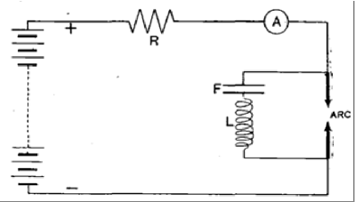
Figure 1: Singing arc circuit diagram [Duddell, 1900a, p. 248]

In fact, Duddell had invented an oscillating circuit susceptible to produce sounds and more than that: electromagnetic waves. Thus, this apparatus will be used as emitter and receiver for the wireless telegraphy till the advent of the triode. By producing spark, the singing arc or Duddell generated electromagnetic waves highlighted by Hertz experiments [Hertz, 1887].

2.1 The singing arc equation

In the last part of his lectures, Poincaré [Poincaré, 1908, p. 390] focused on the maintained oscillations in a singing arc circuit. The circuit diagram he studied (see Fig. 2) is completely identical to that of Duddell (see Fig. 1).

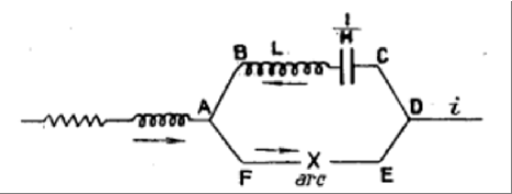
Figure 2: Maintained oscillations in the singing arc [Poincaré, 1908, p. 390]

According to Poincaré [Poincaré, 1908, p. 390] this circuit consists of an Electro Motive Force (E.M.F.) of direct current E, a resistance R and a self, and in parallel, a singing arc and another self L and a capacitor. In order to provide the differential equation modeling the maintained oscillations he calls $x$ the capacitor charge and $i$ the current in the external circuit. Thus, the intensity in the branch (ABCD) comprising the capacitor of capacity $1/H$ may be written:

$$x^{\prime}=\frac{dx}{dt}$$

The current intensity $i_{a}$ in the branch (AFED) comprising the singing may be written while using Kirchoff’s law: $i_{a}=i+x^{\prime}$. Then, Poincaré establishes the following second order nonlinear differential equation for the maintained oscillations in the singing arc:

$$Lx^{\prime\prime}+\rho x^{\prime}+\varphi\left(i+x^{\prime}\right)+Hx=0$$ (1)

He specifies that the term $\rho x^{\prime}$ corresponds to the internal resistance of the self and various damping while the term $\varphi\left(i+x^{\prime}\right)$ represents the E.M.F. of the arc which is related to the intensity by a function, unknown at that time. The main problem of equation (1) is that it depends on two variables $x$ and $i$. So, it is necessary for Poincaré to get rid of $i$.

By neglecting the external self and while equaling the tension in all branches of the circuit he finds that:

$$Ri+\varphi\left(i+x^{\prime}\right)=E$$ (2)

He explains that if the function $\varphi$ was known, equation (2) would provide a relation between $i$ and $x^{\prime}$ or between $i+x^{\prime}$ and $x$ and then the variable $i$ could be eliminated in the equation (1). Thus, he makes the assumption that there exists a function relating $i$ and $x^{\prime}$. Then, he directly replaces in equation (1) $\varphi\left(i+x^{\prime}\right)$ by $\theta\left(x^{\prime}\right)$ and writes:

$$Lx^{\prime\prime}+\rho x^{\prime}+\theta\left(x^{\prime}\right)+Hx=0$$ (3)

2.2 Stability condition: Maintained oscillations and limit cycles

Then, Poincaré establishes, twenty years before Andronov [Andronov, 1929], that the stability of the periodic solution of equation (3) depends on the existence of a “closed curve”, i.e. a stable limit cycle in the phase plane. By using the variable changes he has introduced in his famous memoirs entitled: “Sur les courbes d’éfinis par une équation différentielle” [Poincaré, 1886, p. 168] he sets:

$$x^{\prime}=\frac{dx}{dt}=y\quad\mbox{;}\quad dt=\frac{dx}{dy}=y\quad\mbox{;}\quad x^{\prime\prime}=\frac{dy}{dt}=\frac{ydy}{dx}$$

Thus, equation (3) becomes:

$$Ly\frac{dy}{dx}+\rho y+\theta\left(y\right)+Hx=0$$ (4)

Poincaré states then that:

“Les oscillations entretenues correspondent aux

courbes fermées, s’il y en a.[Poincaré, 1908]”

and he gives the following representation for the solution of equation (4):

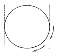
Figure 3: Closed curve solution of equation (4) [Poincaré, 1908, p. 390]

Let’s notice that this closed curve is only a “metaphor” of the solution since Poincaré do not use any graphical integration method such as “isoclines”. Moreover, the main purpose of this representation is to specify the sense of rotation of the trajectory curve which is a preliminary necessary condition to the establishment of the following proof involving the Green-Ostrogradsky theorem.

Then, Poincaré explains that if $y=0$ then $dy/dx$ is infinite and so, the curve admits vertical tangents. Moreover, if $x$ decreases $x^{\prime}$, i.e. $y$ is negative. He concludes that the trajectory curves turns in the direction indicated by the arrow (see Fig. 3).

Poincaré writes:

“Condition de stabilité. - Considérons donc une autre courbe non fermée satisfaisant à l’équation différentielle, ce sera une sorte de spirale se rapprochant indéfiniment de la courbe fermée. Si la courbe fermée représente un régime stable, en décrivant la spirale dans le sens de la flèche on doit être ramené sur la courbe fermée, et c’est à cette seule condition que la courbe fermée représentera un régime stable d’ondes entretenues et donnera lieu à la solution du problème.” [Poincaré, 1908, p. 391]

In the Notice sur les Travaux scientifiques d’Henri Poincaré he wrote in 1886, he defines the concept of limit cycle:

“J’appelle ainsi les courbes fermées qui satisfont à notre équation différentielle et dont les autres courbes définies par la même équation se rapprochent asymptotiquement sans jamais les atteindre.” [Poincaré, 1886n, p. 30]

By comparing both definitions it clearly appears that the “closed curve” which represents a stable regime of maintained oscillations is nothing else but a limit cycle as Poincaré has defined it in his own works. But this, first “giant step” is not sufficient to prove the stability of the oscillating regime. Poincaré has to demonstrate now that the periodic solution of equation (3) (the “closed curve”) corresponds to a stable limit cycle.

2.3 Possibility condition of the problem: stability of limit cycles

In the following part of his lectures, Poincaré gives what he calls a “condition de possibilité du problème”. In fact, he establishes a condition of stability of the periodic solution of equation (3), i.e. a condition of stability of the limit cycle under the form of inequality.

After multiplying equation (4) by $x^{\prime}dt$ Poincaré integrates it over one period while taking into account that the first and fourth term are vanishing since they correspond to the conservative part of this nonlinear equation. He finds:

$$\rho\int{{x}^{\prime 2}dt}+\int{\theta\left({{x}^{\prime}}\right){x}^{\prime}dt}=0$$ (5)

Then, he explains that since the first term is quadratic, the second one must be negative in order to satisfy this equality. So, he stated that the oscillating regime is stable iff:

$$\int{\theta\left({{x}^{\prime}}\right){x}^{\prime}dt}<0$$ (6)

It will be shown in the next section that this inequality is completely identical to the one Andronov [Andronov, 1929] will state twenty years later.

3 Andronov’s works on self-oscillations

In 1920, Aleksandr Aleksandrovich Andronov (1901-1952) entered the Electrical Engineering Department of the Technical High-School of Moscow where a radio engineering specialization was proposed. Five years later, he obtained a diploma in Theoretical Physics (Master Degree) at the university of Moscow. Then, he started a Ph-D with Leonid Isaakovich Mandel’shtam (1879-1944). This charismatic figure which is at the origin of the concept of “nonlinear thinking” has deeply influenced the young Andronov. In fact, the correspondence he established in the famous note at the Comptes Rendus was preceded by a short presentation of his Ph-D works at the sixth congress of Russian Physicists at Moscow between the $5^{th}$ and $16^{th}$ August 1928 [Andronov, 1928]. In this work Andronov gives the foundations of what will become the theory of nonlinear oscillations.

“However, any sufficiently rigorous general theory for such oscillations does not exist nowadays. Meanwhile, there is an adequate mathematical model or schema, created without any connection with the theory of oscillations, which allows a common view of all these processes to the case of one degree of freedom. This concept is the “theory of limit cycles” of Poincaré.” [Andronov, 1928, p. 23]

In his conclusion, which should be compared to that of Poincaré [Poincaré, 1908, p. 391] (See above p. 6), Andronov introduced his famous neologism:

“The stable motions existing in devices capable of self-oscillations must always correspond to limit cycles.”[Andronov, 1928, p. 24]

On Monday, October $14^{th}$, 1929 the French mathematician Jacques Hadamard (1865-1963) presented to the Academy of Sciences of Paris a note from Alexander Andronov. The fact that Hadamard had presented this work is not really surprising since on the one hand he was responsible for mathematical analysis section at the Academy of Sciences and on the other hand he was also correspondent of the Russian Academy of Sciences since 1922 and a foreign member of the Academy of Sciences of the USSR since 1929. In this work, Andronov considers first many examples of non-conservative systems such as the problem of Cepheids for P.D.E., the Froude pendulum and the triode oscillator for nonlinear O.D.E.

“Citons, pour le cas des équations aux dérivées partielles, le problème déjà ancien de la corde vibrante excitée par un archet ainsi que le problème des Céphéides, tel que le traite Eddington $(^{1})$; pour celui des équations différentielles ordinaires, en mécanique le pendule de Froude $(^{2})$, en physique l’oscillateur à triode $(^{3})$, en chimie les réactions périodiques $(^{4})$; des problèmes similaires se posent en biologie $(^{5})$.”

(1) EDDINGTON, The internal constitution of stars, p. 200 (Cambridge, 1926).
(2) Lord RAYLEIGH, The theory of sound, London 1, 1894, p. 212.
(3) Voir par exemple VAN DER POL, Phil. Mag., 7 série, 2, 1926, p. 978. (4) Voir par exemple KREMANN, Die periodischen Erscheinungen in der Chemie, p. 124 (Stuttgart, 1913).
(5) LOTKA, Elements of physical biology, p. 88 (Baltimore, 1925). Voir aussi les récentes recherches de M. Volterra.

[Andronov, 1929, p. 560]

3.1 Self-oscillations and limit cycles

Then, Andronov explains that such systems he calls “self-oscillators“ can be represented in the phase plane by two simultaneous differential equations:

$$\frac{dx}{dt}=P\left(x,y\right)\quad\mbox{;}\quad\frac{dy}{dt}=Q\left(x,y\right)$$ (7)

and he adds that:

“It may easily be shown that, to periodic motions satisfying these conditions, there correspond, in the $xy$ plane, isolated closed curves, approached in spiral fashion by neighboring solutions from the interior or the exterior (for increasing $t$). As a result, self-oscillations arising in systems characterized by equations of type (7) correspond mathematically to stable Poincaré limit cycles $(^{3})$.

$(^{3})$ POINCARÉ, OEuvres, I, p. 53 (Paris, 1928)

[Andronov, 1929, p. 560]

It is important to notice, on the one hand, that due to the imposed format of the Comptes Rendus, Andronov does not provide any demonstration. He just claims that the periodic solution of a non-linear second order differential equation defined by (7) “corresponds” to stable Poincaré limit cycles. On the other hand, it is interesting to compare this sentence with that of Poincaré (See above p. 7). Then, it clearly appears that Andronov has stated the same correspondence as Poincaré twenty years after him. Nevertheless, it seems that Andronov may not have read Poincaré’s article since at that time even if the first volume of his complete works had been already published it didn’t contained this paper.

3.2 Stability condition of limit cycles

The next step for Andronov is to show that the periodic solution, i.e. the limit cycle is stable. To this purpose he considers the following system, where $\mu$ is a real parameter, as an example:

$$\frac{dx}{dt}=y+\mu f\left(x,y;\mu\right)\quad\mbox{;}\quad\frac{dy}{dt}=-x+\mu g\left(x,y;\mu\right)$$ (8)

He explains that for $\mu=0$ the solution of this system is: $x=R\cos\left(t\right)$, $y=R\sin\left(t\right)$ as it is obvious to check. This enables him to introduce an “unusual” variables changes in polar coordinates. Then, by using Poincaré’s methods [Poincaré, 1892-93-99, tome I, p. 89] he states that for sufficiently small $\mu\neq 0$, the $xy$ plane contains only isolated closed curves, near to circles with radii defined by the equation:

$$\int_{0}^{2\pi}\left[f\left(R\cos\xi,-R\sin\xi;0\right)\cos\xi-g\left(R\cos\xi,-R\sin\xi;0\right)\sin\xi\right]d\xi=0$$ (9)

Andronov provides a stability condition for the steady-state motion, i.e. for the limit cycle:

$$\int_{0}^{2\pi}\left[f_{x}\left(R\cos\xi,-R\sin\xi;0\right)\cos\xi+g_{y}\left(R\cos\xi,-R\sin\xi;0\right)\sin\xi\right]d\xi<0$$ (10)

In fact, this condition is based on the use of characteristic exponents introduced by Poincaré in his so-called New Methods on Celestial Mechanics [Poincaré, 1892-93-99, tome I, p. 161] and after by Lyapounov in his famous textbook General Problem of Stability of the Motion [Lyapounov, 1907]. That’s the reason why Andronov will call later the stability condition (10): stability in the sense of Lyapounov or Lyapounov stability. It will be stated in the next section that both stability condition of Poincaré (6) and of Andronov (10) are totally identical.

4 Poincaré stability versus Lyapounov stability

In order to establish a comparison between Poincaré’s results and that of Andronov it is necessary to transform Eq. (4) into a dimensionless system. This can be easily done by using this variables changes: $x\rightarrow\sqrt{L/H}$, $t\rightarrow\mu t$ and while posing: $\mu=1/{\sqrt{LH}}$. Then, starting from Eq. (4) and by neglecting the resistance $\rho$ of the self we have:

$$\left\{\begin{array}[]{l}\dfrac{dx}{dt}=y\vspace{4pt}\\ \dfrac{dy}{dt}=-x-\mu\theta\left(t\right)\end{array}\right.$$ (11)

By comparing with the system of Andronov (8) we find that: $f\left(x,y;\mu\right)=0$ and $g\left(x,y;\mu\right)=-\theta\left(y\right)$. Moreover, the stability condition (10) is only the rough idea of a theorem which will be formalized later by Pontryagin [Pontryagin, 1934]. This theorem involves the Green’s formula ([Pontryagin, 1934, p. 100]):

$$\int_{\Gamma}f\left(x,y\right)dy-g\left(x,y\right)dx=\iint_{S}\left(f^{\prime}_{x}\left(x,y\right)+g^{\prime}_{y}\left(x,y\right)\right)dxdy$$ (12)

where $\Gamma$ and $S$ design respectively a closed path and a surface. Let’s notice that this theorem may be only stated provided that the sense of rotation on the closed path (curve) has been previously defined or chosen. That’s the reason why Poincaré has accurately specified it (see above p. 5). Then, by using Cartesian coordinates system it may be shown that the stability condition of Andronov (10) reads:

$$\int_{\Gamma}f\left(x,y;\mu\right)\frac{dy}{dt}-g\left(x,y;\mu\right)\frac{dx}{dt}<0$$ (13)

Finally, by replacing in Eq. (13) $f\left(x,y;\mu\right)=0$ and $g\left(x,y;\mu\right)=-\theta\left(y\right)$ and taking into account Poincaré’s variables changes (see above p. 5): $x^{\prime}=dx/dt=y$ we have:

$$\int_{\Gamma}\theta\left(t\right)x^{\prime}dt<0$$ (14)

This condition (14) exactly transcribes the fact that the characteristic exponent or Lyapounov exponent is negative. So, the identity between both Poincaré and Andronov stability conditions is thus stated. Then, it appears that Poincaré had not only established a correspondence between maintained oscillations and the existence of a limit cycle but he had also proved the stability of this limit cycle through a condition that Andronov will find again (independently) two decades later.

5 Discussion

In this paper it has been proved that Poincaré in these “forgotten” conferences has established two correspondences between technical problems of oscillations coming from wireless telegraphy and his own works. As well as Andronov in his note at the Comptes Rendus. Indeed, both of them have used, on the one hand, the concept of limit cycle that Poincaré had introduced in his famous memoirs and, on the other hand, the concept of characteristic exponents he had developed for Celestial Mechanics (especially for periodic orbits) in his so-called New Methods.

But, while the former only represents a minor step towards the theory of nonlinear oscillations, because if the limit cycle is unstable no maintained oscillations can be observed, the later is of fundamental importance. It is very surprising to notice that many historians of science have only focussed on the former weakening thus the impact of this result. Moreover, it is difficult to explain why these conferences have been completely ”forgotten” by both scientists and historians over more than a century.

Many hypotheses are to be considered. The main reason is probably that these conferences have never been published in Poincaré’s complete works, only in the journal La Lumière électrique (which disappeared in 1916) and in a textbook. Moreover, they clearly tackle technological problems that are the concern of engineers rather than mathematicians. Papers referring specifically to these conferences address the question of diffraction of radio waves, not maintained oscillations.

No reference to these conferences has been found until today in the technological neither mathematical literature. But other hypotheses must be stated. First it may be reminded that Poincaré studies the singing arc circuit and not the triode circuit. But, after 1920 the singing arc is considered as completely obsolete by engineers, maybe explaining partly that nobody cares about the result of 1908. Except the fact that both singing arc and triode are analogous devices and are so modeled by the same equations, but was this known largely in the 1920s?

Second is the fact that the conferences aimed at presenting the solution of a very “difficult” problem in 1908 to students in telegraphy engineering: the public did not have a high mathematical background, except for the curious who may have attended it. Considering also that during the war, which started in 1914, most of those students may have been killed and the memory of this work may have disappeared in the trenches.

For now, many questions are unresolved. For example: why Poincaré did not use the terminology limit cycle while he gives a very accurate definition of the closed curve towards which any non-closed curve tends? Is it why the audience was supposed to be engineers without basic notions of qualitative theory of differential equations? The problem is that we ignore who was precisely that day in the audience, and have no idea who may have read the texts, who may get inspired with it (without citing it).

In any case, it remains clear that this work of 1908 represents the first application of Poincaré research (on what is called today dynamical system) in a technological problem, anticipating thus the development of the theory of nonlinear oscillations in the twentieth century.

References

- [Aubin & Dahan, 2002] Aubin D. & Dahan-Dalmedico A. [2002] Writing the History of Dynamical Systems and Chaos: Longue Durée and Revolution, Disciplines and Cultures, Historia Mathematica 29, pp. 273-339.
- [Andronov, 1928] Andronov A. A. [1928] Poincaré’s limit cycles and the theory of oscillations (in Russian), n IVs’ezd ruskikh fizikov, 5-16.08, Moscow: N.-Novgorod, Kazan, Saratov, pp. 23-24. (reprinted in Andronov, 1956, p. 32-33)
- [Andronov, 1929] Andronov A. A. [1929] Les cycles limites de Poincaré et la théorie des oscillations auto-entretenues, Comptes Rendus Hebdomadaires de l’Académie des Sciences 189, pp. 559-561.
- [Ayrton, 1902] Ayrton H. [1902] The Electric Arc, (Printing and Publishing Company, London).
- [Barkhausen, 1907] Barkhausen H. [1907] Das Problem der Schwingungserzeugung mit besonderer Berücksichtigung schneller elektrischer Schwingungen, (S. Hirzel, Leipzig).
- [Duddell, 1900a] Du Bois Duddell W. [1900a] On Rapid Variations in the Current through the Direct-Current Arc, Journ. Inst. Elec. Eng. 30, pp. 232-283, (december 13th 1900).
- [Duddell, 1900b] Du Bois Duddell W. [1900b] On Rapid Variations in the Current through the Direct-Current Arc, Journ. Inst. Elec. Eng. 46, pp. 269-273 & pp. 310-313, (december 14th & 21th 1900).
- [Hertz, 1887] Hertz H. R. [1887] Ueber sehr schnelle electrische Schwingungen, Annalen der Physik, vol. 267 (7), pp. 421-448.
- [Janet, 1919] Janet P. [1919] Sur une analogie électrotechnique des oscillations entretenues, Comptes Rendus Hebdomadaires de l’Académie des Sciences 168, pp. 764-766.
- [Lyapounov, 1907] Lyapounov A. [1907] Problème général de la stabilité du mouvement, Annales de la faculté des sciences de Toulouse, Sér. 2 9 (1907), p. 203-474. (Originally published in Russian in 1892. Translated by M. Édouard Davaux, Engineer in the French Navy à Toulon).
- [Mandel’shtam et al., 1935] Mandel’shtam L. I., Papaleksi N. D., Andronov A. A., Khaikin S. E. & Witt A. A. [1935] Exposé des recherches récentes sur les oscillations non-linéaires, Journal de Physique Technique de l’U.R.S.S. 2, p. 81-134 (in French).
- [Massau, 1887] Massau J. [1887] Mémoire sur l’intégration graphique et ses applications, Annales de l’Association des ingénieurs sortis des écoles spéciales de Gand 10, pp. 1-535.
- [Maz’ya & Shaposhnikova, 1998] Maz’ya V. & Shaposhnikova T. O. [1998] Jacques Hadamard: a Universal Mathematician, (History of Mathematics, vol. 14. AMS, Providence, RI, London Mathematical Society).
- [Minorsky, 1947] Minorsky N. [1947] Introduction to Non-Linear Mechanics, (J. W. Edwards, Ann. Arbor, Michigan).
- [Pechenkin, 2002] Pechenkin A. [2002] The concept of self-oscillations and the rise of synergetics ideas in the theory of nonlinear oscillations, Studies in History and Philosophy of Modern Physics 33, pp. 269-295.
- [Poincaré, 1881] Poincaré, H. [1881] Sur les courbes définies par une équation différentielle, J. de Math. Pures et Appl., Série III 7, pp. 375-422.
- [Poincaré, 1882] Poincaré, H. [1882] Sur les courbes définies par une équation différentielle, J. de Math Pures Appl., Série III 8, pp. 251-296.
- [Poincaré, 1885] Poincaré, H. [1885] Sur les courbes définies par une équation différentielle, J. de Math. Pures et Appl., Série IV 1, pp. 167-244.
- [Poincaré, 1886] Poincaré, H. [1886] Sur les courbes définies par une équation différentielle, J. de Math. Pures et Appl., Série IV 2, pp. 151-217.
- [Poincaré, 1886n] Poincaré H. [1886n] Notice sur les Travaux Scientifiques de Henri Poincaré, (Gauthier-Villars, Paris).
- [Poincaré, 1892-93-99] Poincaré H. [1892-93-99] Les Méthodes Nouvelles de la Mécanique Céleste, (Gauthier-Villars, Paris).
- [Poincaré, 1893] Poincaré H. [1893] Sur la propagation de l’électricité, Comptes Rendus Hebdomadaires de l’Académie des Sciences 117, pp. 1027-1032.
- [Poincaré, 1894] Poincaré H. [1894] Les oscillations électriques, (Charles Maurain, G. Carré & C. Naud, Paris).
- [Poincaré, 1899] Poincaré H. [1899] La Théorie de Maxwell et les oscillations Hertziennes, (Charles Maurain, G. Carré & C. Naud, Paris).
- [Poincaré, 1901] Poincaré H. [1901] Sur les excitateurs et résonateurs hertziens (à propos d’un article de M. Johnson), Éclairage électrique 29, pp. 305-307.
- [Poincaré, 1902] Poincaré H. [1902] Sur la télégraphie sans fil, Revue scientifique 17 (375), pp. 65-73.
- [Poincaré, 1903] Poincaré H. [1903] Sur la diffraction des ondes électriques: A propos d’un article de M. Macdonald, Proceedings of the Royal Society of London 72, pp. 42-52.
- [Poincaré, 1904] Poincaré H. [1904] Étude de la propagation du courant en période variable sur une ligne munie de récepteur, Éclairage électrique 40, pp. 121-128, pp. 161-167, pp. 201-212 & pp. 241-250.
- [Poincaré, 1907] Poincaré H. [1907] Sur quelques théorèmes généraux relatifs à l’électrotechnique, Éclairage électrique 50, pp. 293-301.
- [Poincaré, 1908] Poincaré H. [1908] Sur la télégraphie sans fil, Lumière électrique 4, pp. 259-266, pp. 291-297, pp. 323-327, pp. 355-359 & pp. 387-393.
- [Poincaré, 1909a] Poincaré H. [1909a] Les ondes hertziennes et l’équation de Fredholm, Comptes Rendus Hebdomadaires de l’Académie des Sciences 148, pp. 459-453.
- [Poincaré, 1909b] Poincaré H. [1909b] Sur la diffraction des ondes hertziennes, Comptes Rendus Hebdomadaires de l’Académie des Sciences 148, pp. 966-968.
- [Poincaré, 1909c] Poincaré H. [1909c] Sur la diffraction des ondes hertziennes, Comptes Rendus Hebdomadaires de l’Académie des Sciences 149, pp. 621-622.
- [Poincaré, 1909d] Poincaré H. [1909d] Conférences sur la télégraphie sans fil, (Éds. Lumière électrique, Paris).
- [Poincaré, 1909e] Poincaré H. [1909e] La télégraphie sans fil, Journal de l’Université des Annales 3, pp. 541-552.
- [Poincaré, 1910a] Poincaré H. [1910a] Sur l’envoi de l’heure par la télégraphie sans fil, Comptes Rendus Hebdomadaires de l’Académie des Sciences 151, pp. 911.
- [Poincaré, 1910b] Poincaré H. [1910b] Sur la diffraction des ondes hertziennes, Lumière électrique 10, pp. 355-362 & pp. 387-394. Lumière électrique 11, pp. 7-12.
- [Poincaré, 1910c] Poincaré H. [1910c] Sur la diffraction des ondes hertziennes, Rendiconti del Circolo Matematico di Palermo 29, pp. 169-259.
- [Poincaré, 1911] Poincaré H. [1911] Sur diverses questions relatives à la télégraphie sans fil, Lumière électrique 13, pp. 7-12, pp. 35-40, pp. 67-72 & pp. 99-104.
- [Poincaré, 1912] Poincaré H. [1912] Sur la diffraction des ondes hertziennes, Comptes Rendus Hebdomadaires de l’Académie des Sciences 154, pp. 795-797.
- [Pontryagin, 1934] Pontryagin L. S. [1934] On dynamical systems close to Hamiltonian systems, Zh. Éksper. Teoret. 4, pp. 883-885. (English translation)
- [Rytov, 1957] Rytov S. M. [1957] Developments of the theory of nonlinear oscillations in the USSR, Radiotekh. i elektronika, 2 (1435) pp. 169-192.
- [Thomson, 1853] Thomson W. aka Lord Kelvin [1853] On transient electric currents, The London, Edinburgh, and Dublin Philosophical Magazine and Journal of Science, 4 (5), pp. 393-405.
- [van Bladel, 2006] van Bladel J. [2006] http://ursiweb.intec.ugent.be/, pp. 1-12.
- [Van der Pol, 1926] Van der Pol B. [1926] On “relaxation-oscillations”, The London, Edinburgh, and Dublin Philosophical Magazine and Journal of Science 7 (2), pp. 978-992.
- [Whittaker, 1951-53] Whittaker E. T. [1951-53] A History of the Theories of Aether and Electricity, (2 vols, T. Nelson, London).