“Super-Kilonovae” from Massive Collapsars as Signatures of Black-Hole Birth
in the Pair-instability Mass Gap

Abstract

The core collapse of rapidly rotating massive $\sim 10M_{\odot}$ stars (“collapsars”), and resulting formation of hyper-accreting black holes, are a leading model for the central engines of long-duration gamma-ray bursts (GRB) and promising sources of $r$-process nucleosynthesis. Here, we explore the signatures of collapsars from progenitors with extremely massive helium cores $\gtrsim 130M_{\odot}$ above the pair-instability mass gap. While rapid collapse to a black hole likely precludes a prompt explosion in these systems, we demonstrate that disk outflows can generate a large quantity (up to $\gtrsim 50M_{\odot}$) of ejecta, comprised of $\gtrsim 5-10M_{\odot}$ in $r$-process elements and $\sim 0.1-1M_{\odot}$ of ⁵⁶Ni, expanding at velocities $\sim 0.1$ c. Radioactive heating of the disk-wind ejecta powers an optical/infrared transient, with a characteristic luminosity $\sim 10^{42}$ erg s^-1 and spectral peak in the near-infrared (due to the high optical/UV opacities of lanthanide elements) similar to kilonovae from neutron star mergers, but with longer durations $\gtrsim$ 1 month. These “super-kilonovae” (superKNe) herald the birth of massive black holes $\gtrsim 60M_{\odot}$, which—as a result of disk wind mass-loss—can populate the pair-instability mass gap “from above” and could potentially create the binary components of GW190521. SuperKNe could be discovered via wide-field surveys such as those planned with the Roman Space Telescope or via late-time infrared follow-up observations of extremely energetic GRBs. Gravitational waves of frequency $\sim 0.1-50$ Hz from non-axisymmetric instabilities in self-gravitating massive collapsar disks are potentially detectable by proposed third-generation intermediate and high-frequency observatories at distances up to hundreds of Mpc; in contrast to the “chirp” from binary mergers, the collapsar gravitational-wave signal decreases in frequency as the disk radius grows (“sad trombone”).

1 Introduction

The astrophysical locations which give rise to the synthesis of heavy nuclei via the rapid capture of neutrons onto lighter seed nuclei (the $r$-process; Burbidge et al. 1957; Cameron 1957) remains a topic of active debate (see Horowitz et al. 2019; Cowan et al. 2021; Siegel 2021 for recent reviews). Several lines of evidence, ranging from measurements of radioactive isotopes on the sea floor (e.g., Wallner et al. 2015; Hotokezaka et al. 2015) to the abundances of metal-poor stars formed in the smallest dwarf galaxies (e.g., Ji et al. 2016; Tsujimoto et al. 2017), suggest that the dominant site of the $r$-process is much rarer than ordinary core collapse supernovae (SNe), both in the early history of our Galaxy and today. The most promising contenders are the mergers of neutron star binaries (e.g., Lattimer & Schramm 1974; Symbalisty & Schramm 1982) or rare channels of core collapse SNe, such as those which give birth to a rapidly spinning magnetar (Thompson et al., 2004; Metzger et al., 2007; Winteler et al., 2012; Nishimura et al., 2015) or a hyper-accreting black hole (“collapsar”; e.g., Surman et al. 2008; Siegel et al. 2019; see also Grichener & Soker 2019). Perhaps not coincidentally, the same two types of events$-$neutron star mergers and collapsars$-$are the leading models for the central engines of gamma-ray bursts (GRB) of the short- and long-duration classes, respectively (e.g., Woosley & Bloom 2006; Berger 2014).

The radioactive decay of $r$-process elements in the ejecta of a neutron star mergers power a short-lived optical/infrared transient known as a kilonova (Li & Paczyński, 1998; Metzger et al., 2010; Barnes & Kasen, 2013). However, the large quantity of $r$-process ejecta $\gtrsim 0.02-0.06M_{\odot}$ inferred from the kilonova to accompany GW170817, as well as the relatively low inferred outflow velocity $\sim 0.1$ c of the bulk of this material (e.g., Cowperthwaite et al. 2017; Drout et al. 2017; Villar et al. 2017), do not agree with predictions from numerical relativity for the mass ejected during the early dynamical phase of the merger (see Metzger 2019; Siegel 2019; Margutti & Chornock 2020; Nakar 2020 for reviews). Instead, the dominant ejecta source in GW170817, and likely in the majority of neutron star mergers, are delayed outflows from the accretion disk which forms around the black hole (BH) or neutron star remnant (e.g., Metzger et al. 2008; Fernández & Metzger 2013; Just et al. 2015; Siegel & Metzger 2017, 2018; Fujibayashi et al. 2018). General relativistic magnetohydrodynamical (GRMHD) simulations of the long-term evolution of post-merger disk find that up to $\sim 30\%$ of its original mass is unbound in outflows with average velocities $\sim 0.1$ c (Siegel & Metzger, 2017; Fujibayashi et al., 2018; Fernández et al., 2019; Christie et al., 2019; Fujibayashi et al., 2020), broadly consistent with the kilonova observed from GW170817.

As emphasized by Siegel, Barnes, & Metzger (2019), similar accretion disk outflows to those generated in neutron star mergers occur also in collapsars (see also MacFadyen & Woosley 1999; Janiuk et al. 2004; Surman et al. 2006; Miller et al. 2020; Just et al. 2021). Unlike in the merger case, the collapsing stellar material feeding the disk is composed of roughly equal numbers of protons and neutrons (electron fraction $Y_{e}\simeq 0.5$). However, for mass accretion rates above a critical threshold value ($\gtrsim 10^{-1}-10^{-3}M_{\odot}$ s^-1, which depends on the effective viscosity and BH mass; Chen & Beloborodov 2007; Metzger et al. 2008), the inner regions of the disk are electron degenerate and act to “self-neutronize” via electron captures on protons (e.g., Beloborodov 2003), thus maintaining a low electron fraction $Y_{e}\approx 0.1$ in a regulated process (Siegel & Metzger, 2017). As a result, the collapsar disk outflows, which feed on this neutron-rich reservoir, can themselves possess a sufficiently high neutron concentration to enable an $r$-process, throughout much of the epoch over which the GRB jet is being powered. However, the details of the synthesized composition$-$particularly the partitioning between light and heavy $r$-process elements$-$are sensitive to the impact of neutrino absorption processes on the electron fraction of the outflowing material (Surman et al. 2006; Miller et al. 2020; Li & Siegel 2021).

In comparison to neutron star mergers, collapsars hold several complementary advantages as $r$-process sources (Siegel et al., 2019). Firstly, as a result of being generated promptly from very massive stars and empirically found to occur in small dwarf galaxies at low metallicity (e.g., Fruchter et al. 2006), collapsars naturally explain the $r$-process enrichment in ultra-faint dwarf galaxies such as Reticulum II (e.g., Ji et al. 2016) and metal-poor stars in the Galactic halo (e.g., Brauer et al. 2021). Furthermore, if the gamma-ray luminosity of GRBs scales with BH accretion rate in the same way in mergers as in collapsars, then from the relative rate and gamma-ray fluence distributions of long- versus short-duration GRBs, one is led to conclude that the total mass accreted through collapsar disks over cosmic time (and hence the integrated amount of disk wind ejecta) could exceed that in neutron star mergers (Siegel et al., 2019). Arguments based on the chemical evolution history of the early Milky Way galaxy have been made both in favor of rare SNe/collapsars (Côté et al., 2019; Siegel et al., 2019; van de Voort et al., 2020; Yamazaki et al., 2021; Brauer et al., 2021) and mergers (Shen et al., 2015; Duggan et al., 2018; Macias & Ramirez-Ruiz, 2019; Bartos & Márka, 2019; Holmbeck et al., 2019; Tarumi et al., 2021) as sources of early $r$-process.

While the kilonova from GW170817 provided ample evidence that neutron star mergers can execute an $r$-process, the same signature has not yet been seen from the SNe observed in coincidence with long GRBs. However, this fact is not necessarily constraining yet, insofar that $r$-process material is easier to hide in the collapsar case. In particular, a prompt and powerful supernova explosion may be required to explain the large masses of ⁵⁶Ni inferred from GRB supernova light curves (e.g., Cano 2016; Barnes et al. 2018; however, see Zenati et al. 2020). By contrast, the $r$-process-generating disk outflows occur over longer times, up to tens of seconds or more after collapse, commensurate with the observed duration of the long GRB. Unless efficiently mixed to the highest velocities, the $r$-process elements (and any associated photometric or spectroscopic signatures) are therefore buried behind several solar masses of “ordinary” supernova ejecta (dominated by $\alpha$-elements such as oxygen).

Nevertheless, if present in the inner ejecta layers, $r$-process elements could manifest as a late-time infrared signal (Siegel et al., 2019) arising from the high opacity of heavy $r$-process nuclei (Kasen et al., 2013; Tanaka & Hotokezaka, 2013). This signal is challenging to detect given the typically large distances to GRB SNe and the late times required (at which point the emission is faint). The detection prospects will improve with the advent of the James Webb Space Telescope (JWST), particularly if the nebular spectra of lanthanide-rich material also peaks in the infrared (Hotokezaka et al., 2021).

Collapsars of the type observed so far as SNe may also only represent a subset of accretion-powered core collapse events. The progenitor stars which give rise to long GRBs are typically believed to possess ZAMS masses $\lesssim 40M_{\odot}$ with helium cores at death of $\lesssim 10M_{\odot}$ (e.g., Woosley & Heger 2006). Upon collapse of their iron cores, these events first go through a rapidly rotating proto-neutron star phase (Dessart et al., 2008), in which a millisecond magnetar is formed (Thompson & Duncan, 1993; Raynaud et al., 2020). The strong and collimated outflow from such a magnetar during the first seconds after its birth (Thompson et al., 2004; Metzger et al., 2007), before it accretes sufficient matter to collapse into a BH, may play an important role in shock heating and in unbinding much of the outer layers of the star and generating the required large ⁵⁶Ni masses (e.g., Shankar et al. 2021).

On the other hand, the number of long GRBs with detected SNe only number around a dozen, and the majority of these are associated with the volumetrically more common but physically distinct “low luminosity” class of GRBs (e.g., Liang et al. 2007). It thus remains unclear whether the more energetic, classical long GRBs always occur in coincidence with ⁵⁶Ni-powered SNe. Indeed, luminous SNe have been ruled out for a few nominally long GRBs (e.g., Fynbo et al. 2006; Gehrels et al. 2006), though the nature of these events (e.g., whether they are actually short GRBs masquerading as collapsars) remains unclear (e.g., Zhang et al. 2007).

Within this context, we consider in this paper the fate of initially much more massive stars, those with ZAMS masses $M_{\rm ZAMS}\gtrsim 260M_{\odot}$ which are predicted to evolve helium cores by the time of core collapse above the pair-instability (PI) gap $\gtrsim 130M_{\odot}$ (e.g., Woosley et al. 2002, Woosley 2017, Renzo et al. 2020b, Farmer et al. 2020, Woosley & Heger 2021). If the initial mass function (IMF) is an indication, such stars are potentially much rarer than the ordinarily considered collapsar progenitors with $M_{\rm ZAMS}\lesssim 40M_{\odot}$. On the other hand, if such stars are rapidly spinning (e.g., Marchant et al., 2019; Marchant & Moriya, 2020)—possibly because of continuous gas accretion throughout their life (e.g. Jermyn et al., 2021; Dittmann et al., 2021)—and if these form collapsar-like disks upon collapse in proportion to their (much higher) helium core masses, their resulting yield of $r$-process ejecta in disk winds could be substantially greater.

Another key difference is that a prompt explosion (e.g., as attributed to a proto-magnetar above, or fallback accretion; Powell et al. 2021) is more challenging to obtain for these very massive stars. This is because (1) the nominal timescale for BH formation is much faster, within $\lesssim 0.1$ s, due to large masses exceeding $2M_{\odot}$ and high compactness of their iron cores (e.g., Renzo et al., 2020b); (2) their larger $\gtrsim 10^{53}$ erg gravitational binding energies relative to those of lower mass helium cores $\lesssim 10^{52}$ erg exceed the rotational energies of even maximally spinning neutron stars. As a result of the assuredly failed initial explosion of post-PI cores, these systems are unlikely to eject a large quantity of prompt, shock-synthesized ⁵⁶Ni and unprocessed stellar material (however, see Fujibayashi et al. 2021). Instead, the bulk of the ejecta will arise over longer timescales from disk outflows, which–scaling up from low-mass collapsars—could amount to $\gtrsim 10M_{\odot}$ of $r$-process and Fe-group elements (including ⁵⁶Ni).

Rather than the usual picture of GRB SNe, the type of collapse transient above the PI-gap we envision is in some ways more akin to a scaled-up neutron star merger. At risk of committing etymological heresy, we therefore refer to these massive collapsar transient events as “super-kilonovae” (superKNe). As we shall discuss, if superKNe exist, their long durations and red colors may render them potentially identifiable through either follow-up infrared observations of long GRBs (e.g., with JWST), or blindly in surveys with the Vera Rubin Observatory (Tyson 2002) or the Nancy Grace Roman Space Telescope (Roman; Spergel et al. 2015).

The gravitational wave observatory LIGO/Virgo detected a binary BH merger, GW190521, for which both binary components of masses $\sim\!85M_{\odot}$ and $\sim\!66M_{\odot}$, respectively (Abbott et al., 2020), were inside the nominal PI mass gap. Tentative evidence suggests an effective high BH spin of the progenitor binary, albeit with the spin axis misaligned with the orbital momentum axis (however, see Mandel & Fragos 2020; Nitz & Capano 2021). These unusual properties have motivated a number of theoretical studies proposing new ways to populate the PI mass gap, such as through dynamical stellar mergers (e.g. Di Carlo et al., 2019, 2020; Renzo et al., 2020a), hierarchical black hole mergers in dense environments (e.g., Antonini & Rasio 2016; Yang et al. 2019; Tagawa et al. 2021; Gerosa & Fishbach 2021), modifying stellar physics at low metallicity (e.g. Farrell et al., 2021; Vink et al., 2021), or through external gas accretion (e.g., Safarzadeh & Haiman 2020). As we shall describe, if both the BHs acquired their low expected masses and high spin as a result of inefficient disk accretion, superKN events of the type envisioned here provide a novel single-star channel for filling the PI mass gap “from above”.

This paper is organized as follows. Sec. 2 presents a semi-analytic model for the collapse of rotating massive stars, their accretion disks and disk wind ejecta, and resulting heavy element nucleosynthesis, which builds on earlier work in Siegel et al. (2019). Calibrating the model such that collapsars generate BH accretion events consistent with the observed properties of long GRB jets, we then apply the model to more massive $\gtrsim 130M_{\odot}$ progenitors above the PI mass gap. Using our results for the disk wind ejecta, in Sec. 3 we calculate the light curves and spectra of their superKN emission by means of Monte Carlo radiative transfer simulations. Sec. 4 explores the prospects for discovering superKNe by future optical/infrared surveys or in follow-up observations of long GRBs. Section 5 discusses several implications of our findings, including gravitational-wave emission from self-gravitating phases of the collapsar disk evolution; the astrophysical origin of GW190521; and the luminous radio and optical emission that results from the superKN ejecta interacting with surrounding gas. Sec. 6 summarizes our results.

2 Disk Outflow Model

2.1 Stellar models

To model the pre-collapse structure of the superKN progenitors, we employ the MESA stellar evolution models of Renzo et al. (2020b), publicly available at https://zenodo.org/record/3406357. The simulations start from naked helium cores of metallicity $Z=0.001$ which are then self-consistently evolved from helium core ignition, through possible (pulsational) pair-instability (PPI), to the onset of core-collapse (defined as when the radial in-fall velocity exceeds $1000\,\mathrm{km\ s^{-1}}$). We label the input stellar models according to their initial helium core mass, e.g., model 200.25 corresponds to $M_{\rm He,init}=200.25M_{\odot}$, and focus on models “above” the PI gap, which do not experience pair-instability driven pulses.

The models are computed using a 22-isotope nuclear reaction network, which is sufficient to capture the bulk of the energy generation throughout the stellar evolution, but cannot accurately capture the weak-interactions in the innermost core (e.g., Farmer et al., 2016). However, the deepest layers of the core promptly fall into the newly formed BH (see Sec. 2.2) and hence do not contribute to the accretion disk and its outflows.

These models were evolved without rotation, which we instead artificially impose at the point of core collapse (see Sec. 2.2). The main effect of rotation during the pre-core-collapse evolution is mixing at the core-envelope interface, which leads to more massive helium cores for a given initial mass. In the extreme case of chemically homogeneous evolution (Maeder & Meynet, 2000), the entire star may become a helium core. This will impact how many stars develop core masses reaching into the PI/pulsational PI regime or beyond, and thus the predicted population statistics. However, because Renzo et al. (2020b) only simulate the helium core, this does not affect our present study. Rotation can also enhance the wind mass-loss rate (e.g., Langer, 1998), and increase the radius in the outer layers at the rotational equator by up to 50%, which is neglected in the progenitors we use. Finally, by adding centrifugal support to the core, rotation can modestly increase the PI/pulsational PI mass range (e.g., Glatzel et al., 1985).

For sufficiently large initial core masses $M_{\mathrm{He,init}}\gtrsim 200\,M_{\odot}$, the final mass at collapse would nominally produce a BH above the PI mass gap (neglecting subsequent mass-loss in accretion disk outflows, as explored in the present study). This arises because the gravitational energy released by the PI-driven collapse acts to photo-disintegrate nuclei produced in the thermonuclear explosion, instead of generating outwards bulk motion (e.g., Bond et al., 1984). Since these models do not experience pulses of mass loss, their pre-collapse total mass is determined by the assumed wind mass-loss prescription: the minimum final helium core mass above the PI mass gap for our MESA models is $M_{\mathrm{He,fin}}\gtrsim 125\,M_{\odot}$. Renzo et al. (2020b) estimated the corresponding final BH mass (again, neglecting post-collapse disk outflows) as the total baryonic mass with binding energy $<10^{48}$ ergs, which effectively corresponds to the total final mass within a few $0.1\,M_{\odot}$ (e.g., Farmer et al., 2019; Renzo et al., 2020b).

A key ingredient in modeling fallback accretion is the radial density profile of the star at collapse (Sec. 2.2). Despite their large masses, helium stars above the PI gap remain compact throughout their lives, never expanding as a result of PI pulses. Their typical radii $R_{\star}\approx 10\,R_{\odot}$ are similar to the normally considered Wolf-Rayet progenitors of GRBs (e.g., Woosley & Heger 2006; Fig. 1). If stars in this mass range reach core collapse with their hydrogen envelope intact (e.g., for sufficiently low metallicity, as in population III stars) their radii could be considerably larger; however, no red supergiants of this mass have yet been observed.

We also employ the $15\,M_{\odot}$ and $20\,M_{\odot}$ single (hydrogen-rich) star models from Heger et al. (2000) to test our collapsar model on more canonical long-GRB progenitors (see Appendix D for a discussion of results). These are computed starting from a surface equatorial velocity of $200\,\mathrm{km\ s^{-1}}$ at ZAMS and assume that mean molecular weight gradients do not impede rotational mixing ($f_{\mu}=0$, “weak molecular weight barriers”). They are labeled E15 and E20 respectively, and are publicly available at https://2sn.org/stellarevolution/rotation/.

2.2 Collapsar Model

The masses and composition of the superKNe ejecta are computed by modeling the collapse of a progenitor star. Depending on the stellar angular momentum profile, the collapse and fallback of envelope material leads to the formation of an accretion disk, which gives rise to massive neutron-rich disk outflows (Siegel et al., 2019; Miller et al., 2020; Just et al., 2021). Although rotation profiles of massive stars at the time of core collapse, in particular of those above the PI mass gap considered here, are highly uncertain (e.g., Heger et al. 2000; Ma & Fuller 2019; Marchant & Moriya 2020), the specific angular momentum $j_{z}$ generally increases with stellar radius. In-falling stellar material thus circularizes at increasingly larger radii from the BH with time.

We endow the stellar models with mass $M_{\star}$ and radius $R_{\star}=R_{\rm He,fin}$ at the time of core collapse (Sec. 2.1) with an angular momentum profile that assumes rigid rotation on spherical shells, with angular velocity $\Omega(r,\theta)=\Omega(r)$. This results in

$$j_{z}(r,\theta)=j(r)\sin^{2}(\theta),$$ (1)

where $r,\theta$ are the radial and polar angle coordinates, respectively. We adopt a general parametrized angular momentum profile of the form

$$j(r)=\left\{\begin{array}[]{cc}f_{\rm K}j_{\rm K}(r)\left(\frac{r}{r_{\rm b}}\right)^{p},&r<r_{\rm b}\\ f_{\rm K}j_{\rm K}(r),&r_{\rm b}\leq r\leq R_{\star}\end{array}\right.,$$ (2)

where $r_{\rm b}$, $p$, and $f_{\rm K}$ are free parameters. This corresponds to a low-density ‘envelope’, composed primarily of helium in the models considered here, rotating at a fraction $f_{\rm K}<1$ of the local Keplerian angular momentum $j_{\rm K}=\sqrt{GM_{\rm enc}(r)r}$, where $M_{\rm enc}(r)$ is the mass enclosed interior to radius $r$, and an inner ‘core’, in which rotation is suppressed by a power-law with index $p$ relative to the fraction of local break-up rotation adopted for the envelope. Although the parameter values ($r_{\rm b}$, $p$, $f_{\rm K}$) are uncertain, as we discuss below, they can be “calibrated” to produce the timescales and energetics of the disk accretion consistent with the observed properties of long GRB jets. Figure 1 illustrates the parametrized rotation profile for model 250.25.

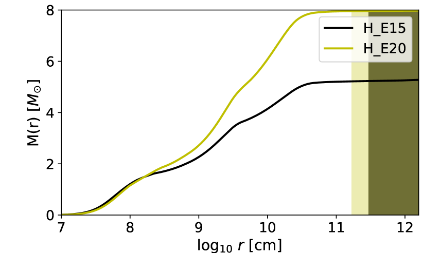
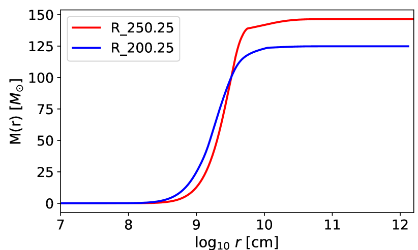
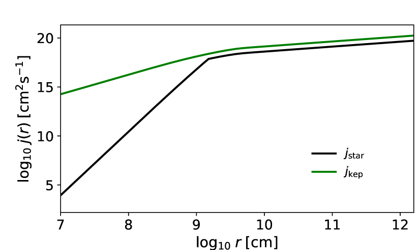
Figure 1: Properties of stellar models at the onset of collapse, showing the enclosed mass as a function of stellar radius (top: models E15 and E20 of Heger et al. 2000; center: models 200.0 and 250.25 of Renzo et al. 2020b), and an example of the imposed specific angular momentum profile for model 250.25 with $p=4.5$, $r_{\rm b}=1.5\times 10^{9}$ cm, and $f_{\rm K}=0.3$ (cf. Eq. 2) compared to the corresponding Keplerian profile (green solid line; bottom). The light (dark) shaded region in the top panel represents the hydrogen envelopes of the E20 (E15) models. Such envelopes are absent in the models of Renzo et al. (2020b).

Assuming an axisymmetric rotating star, we discretize the progenitor stellar model into $(n_{r},n_{\theta})$ mass elements, logarithmically spaced in stellar radius $r$, and uniformly spaced in $\cos\theta$. The angular resolution is chosen sufficiently high (typically $n_{\theta}=1001$) that the accuracy in numerically computing global quantities by integration (total mass, total fall-back mass, etc.) is dominated by the finite radial resolution of the stellar progenitor models. Defining $t=0$ as the onset of core-collapse, a given stellar layer at radius $r$ will start to collapse onto the centre upon the sound travel time $t_{\rm s}(r)=\int_{0}^{r}c_{s}^{-1}(r){\rm d}r$ from the centre to $r$. Due to its finite angular momentum, a given fluid element will do so on an eccentric trajectory and circularize on the equatorial plane at time (cf. Kumar et al. 2008)

$$t_{\rm circ}(r,\theta) = t_{\rm s}(r)$$

$$+ \frac{(1+e)^{-3/2}}{\Omega_{\rm K}(r)}\left[\cos^{-1}(-e)+e(1-e^{2})^{1/2}\right]$$

and radius

$$r_{\rm circ}(r,\theta)=\left(\frac{8}{3\pi}\right)^{2}r(1-e),$$ (4)

where $e(r,\theta)=1-[\Omega^{2}(r)/\Omega^{2}_{\rm K}(r)]\sin^{2}\theta$ is the eccentricity of the trajectory and $\Omega_{\rm K}=(GM_{\rm enc}(r)/r^{3})^{1/2}$ the Keplerian angular velocity.

The innermost parts of the stellar core may not possess sufficient angular momentum to circularize in an accretion disk and, instead, directly collapse into a BH. We define the initial BH as a ‘seed BH’ formed by the innermost stellar layers up to radius $r_{\bullet,0}$ with enclosed mass $M_{\bullet,0}=0.5\,M_{\odot}$, a safe assumption for all stellar models considered here. This seed BH has dimensionless spin parameter

$$a_{\bullet,0}=\frac{cJ_{\rm enc}(r_{\bullet,0})}{GM^{2}_{\rm enc}(r_{\bullet,0})},$$ (5)

where $J_{\rm enc}(r)$ is the enclosed angular momentum, $G$ is the gravitational constant, and $c$ is the speed of light. The corresponding innermost stable circular orbit (ISCO) is given by (Bardeen et al., 1972)

$$r_{\mathrm{ISCO}}(M_{\bullet},a_{\bullet}) = \frac{GM_{\bullet}}{c^{2}}$$

$$\times \left\{3+z_{2}-\left[(3-z_{1})(3+z_{1}+2z_{2})\right]^{1/2}\right\},$$

where

$$z_{1} = 1+(1-a_{\bullet}^{2})^{1/3}\left[(1+a_{\bullet})^{1/3}+(1-a_{\bullet})^{1/3}\right],$$ (7)

$$z_{2} = (3a_{\bullet}^{2}+z_{1}^{2})^{1/2}.$$ (8)

Upon initial BH formation, we follow the collapse of the outer stellar layers according to Eqs. (2.2) and (4) and distinguish between mass elements that circularize outside the BH to form a disk ($r_{\rm circ}(r(t),\theta)>r_{\rm ISCO}(t)$), giving rise to a ‘disk feeding rate’ $\dot{m}_{\rm fb,disk}$, and those that directly fall into the BH without accreting through a disk ($r_{\rm circ}(r(t),\theta)\leq r_{\rm ISCO}(t)$), giving rise to a direct fallback rate onto the BH $\dot{m}_{\rm fb,\bullet}$. Here, $r(t)$ refers to the radius of a stellar element at polar angle $\theta$ which circularizes at time $t$ in the equatorial plane. We denote the associated rates of angular momentum supplied to the disk and the BH by $\dot{J}_{\rm fb,disk}$ and $\dot{J}_{\rm fb,\bullet}$, respectively.

We follow the evolution of the BH, disk, and ejecta properties solving the following equations:

$$\frac{{\rm d}M_{\rm\bullet}}{{\rm d}t} = \dot{m}_{\rm fb,\bullet}+\dot{m}_{\rm acc},$$ (9)

$$\frac{{\rm d}J_{\rm\bullet}}{{\rm d}t} = \dot{J}_{\rm fb,\bullet}+\dot{m}_{\rm acc}j_{\rm ISCO},$$ (10)

$$\frac{{\rm d}M_{\rm disk}}{{\rm d}t} = \dot{m}_{\rm fb,disk}-\dot{m}_{\rm acc}-\dot{m}_{\rm wind},$$ (11)

$$\frac{{\rm d}J_{\rm disk}}{{\rm d}t} = \dot{J}_{\rm fb,disk}-\dot{m}_{\rm acc}j_{\rm ISCO}-\dot{J}_{\rm wind},$$ (12)

$$\frac{{\rm d}M_{\rm ejecta}}{{\rm d}t} = \dot{m}_{\rm wind},$$ (13)

$$\frac{{\rm d}J_{\rm ejecta}}{{\rm d}t} = \dot{J}_{\rm wind}.$$ (14)

Here,

$$j_{\rm ISCO} = (GM_{\rm\bullet}r_{\rm ISCO})^{1/2}\times$$

$$\mskip-40.0mu\frac{r^{2}_{\mathrm{ISCO}}-a_{\rm\bullet}r_{g}(r_{\mathrm{ISCO}}r_{g}/2)^{1/2}+a_{\rm\bullet}^{2}r_{g}^{2}/4}{r_{\mathrm{ISCO}}\left[r^{2}_{\mathrm{ISCO}}-3r_{\mathrm{ISCO}}r_{g}/2+a_{\rm\bullet}r_{g}(r_{\mathrm{ISCO}}r_{g}/2)^{1/2}\right]^{1/2}}$$

is the specific angular momentum of a fluid element at the ISCO of the BH with mass $M_{\rm\bullet}$, spin $a_{\rm\bullet}=cJ_{\rm\bullet}/GM_{\rm\bullet}^{2}$, and gravitational radius $r_{g}=2GM_{\rm\bullet}/c^{2}$ (Bardeen et al., 1972). Mass is accreted onto the BH at a rate

$$\dot{m}_{\rm acc}=f_{\rm acc}\frac{M_{\rm disk}}{t_{\rm visc}},$$ (16)

where

$$t_{\rm visc}=\alpha^{-1}\Omega_{\rm K,disk}^{-1}h_{\rm z,disk}^{-2}$$ (17)

is the viscous timescale of the disk, with $\alpha$ being the standard dimensionless disk viscosity (Shakura & Sunyaev, 1973),

$$\Omega_{\rm K,disk}(t)=(GM_{\rm\bullet}/r_{\rm disk}^{3})^{1/2}$$ (18)

is the Keplerian angular velocity of the disk, and $h_{\rm z,disk}$ its scale height (we take $h_{\rm z,disk}\approx 0.5$ as a fiducial value). The disk radius $r_{\rm disk}(t)$ is defined by the current disk mass and angular momentum,

$$j_{\rm disk}\equiv(GM_{\rm\bullet}r_{\rm disk})^{1/2}=\frac{J_{\rm disk}}{M_{\rm disk}}.$$ (19)

The disk accretion flow gives rise to powerful outflows with mass-loss at a rate

$$\dot{m}_{\rm wind}=(1-f_{\rm acc})\frac{M_{\rm disk}}{t_{\rm visc}},$$ (20)

and associated angular momentum loss rate

$$\dot{J}_{\rm wind}=\dot{m}_{\rm wind}j_{\rm disk}.$$ (21)

Neutrinos cool the disk effectively above the critical “ignition” accretion rate for weak interactions (Chen & Beloborodov, 2007; Metzger et al., 2008; Siegel et al., 2019; De & Siegel, 2020), which is approximately given by (see Appendix A.1)

$$\dot{M}_{\rm ign}\approx 2\times 10^{-3}M_{\odot}{\rm s}^{-1}\left(\frac{\alpha}{0.02}\right)^{5/3}\left(\frac{M_{\rm\bullet}}{3M_{\odot}}\right)^{4/3}.$$ (22)

Motivated by the findings of GRMHD simulations of neutrino-cooled accretion flows (Siegel & Metzger, 2018; Fernández et al., 2019; Siegel et al., 2019; De & Siegel, 2020), we assume that for high accretion rates $>\!\dot{M}_{\rm ign}$ a fraction $1-f_{\rm acc}\approx 0.3$ of the disk mass is unbound in outflows. This fraction is assumed to increase to $\approx 0.6$ below $\dot{M}_{\rm ign}$, under the assumption that inefficient cooling will result in excess heating and outflow production (e.g., Blandford & Begelman 1999; De & Siegel 2020). Similarly, we assume that enhanced outflow production occurs also at very high accretion rates, for which neutrinos become effectively trapped in the optically thick accretion disk and are advected into the BH before radiating. This threshold “trapping” accretion rate is given by (see Appendix A.3)

$$\dot{M}_{\nu,{\rm trap}}\approx 1M_{\odot}{\rm s}^{-1}\left(\frac{\alpha}{0.02}\right)^{1/3}\left(\frac{M_{\rm\bullet}}{3M_{\odot}}\right)^{4/3}.$$ (23)

Insofar as $\dot{M}_{\nu,{\rm trap}}$ scales in the same way with the (growing) BH mass as $\dot{M}_{\rm ign}$, we find this trapped regime is of little practical importance in our models. In summary, the accretion efficiency is given by

$$f_{\rm acc}=\left\{\begin{array}[]{cc}0.4,&\dot{M}_{\nu,{\rm trap}}\leq\frac{M_{\rm disk}}{t_{\rm visc}}\\ 0.7,&\dot{M}_{\rm ign}<\frac{M_{\rm disk}}{t_{\rm visc}}<\dot{M}_{\nu,{\rm trap}}\\ 0.4,&\frac{M_{\rm disk}}{t_{\rm visc}}\leq\dot{M}_{\rm ign}\end{array}\right..$$ (24)

Eqs. (9)–(14) allow a calculation of the total ejecta mass $M_{\rm ejecta}$ obtained from a particular collapsar model. We evolve this set of coupled differential equations numerically until all stellar progenitor material has collapsed and has either been accreted onto the BH or been ejected into outflows. Note that these equations explicitly conserve mass and angular momentum. Time stepping is equidistant in $\log t$ and chosen sufficiently high, such that i) the accuracy of the total fallback mass is dominated by the radial resolution of the provided stellar model (see Appendix C) and that ii) conservation of total mass and angular momentum in Eqs. (9)–(14) is achieved to better than $10^{-14}$ relative accuracy for all model runs.

Once a disk forms around the BH and its accretion rate $\dot{m}_{\rm acc}$ exceeds $10^{-4}\,M_{\odot}\,\text{s}^{-1}$, we assume that a relativistic jet emerges, powerful enough to drill through the remaining outer layers in the polar region. This threshold is motivated by typical GRB luminosities $L_{\gamma}\sim\!2\times 10^{50}\,\text{erg}\,\text{s}^{-1}$ (Goldstein et al., 2016), which, if accretion powered, require an accretion rate of at least $\dot{M}\sim L_{\gamma}/c^{2}\sim 1.1\times 10^{-4}\,M_{\odot}\,\text{s}^{-1}$. If this threshold is surpassed, we ignore any remaining material in the polar regions $\theta<\theta_{\rm jet}$ and $\theta>180^{\circ}-\theta_{\rm jet}$ for the subsequent fallback process. This material has little effect on the total quantity of material accreted through the disk as it predominantly falls into the BH directly due to the low angular momentum in these regions. However, it has a slight indirect effect on nucleosynthesis by modifying the BH mass (see below). As a fiducial value, we take $\theta_{\rm jet}=30^{\circ}$. We further justify the existence of such a successful jet a posteriori by the fact that our models reach the regime $\dot{M}>10^{-4}\,M_{\odot}\,\text{s}^{-1}$ favorable for powering typical observed long GRBs including the time necessary for the jet to drill through the stellar envelope (see Sec. 2.3).

The fallback process may in some cases give rise to massive, gravitationally unstable accretion disks. In this limit, the disk mass becomes comparable to the BH mass, and our assumption of a Kerr metric would not be justified anymore. We estimate this instability region by monitoring the ratio of self-gravity to external gravitational acceleration by the BH potential (Paczynski, 1978; Gammie, 2001),

$$Q^{-1}\equiv\frac{2\pi\Sigma r_{\rm disk}^{2}}{M_{\rm\bullet}h_{z,{\rm disk}}}\simeq\frac{2}{h_{z,{\rm disk}}}\frac{M_{\rm disk}}{M_{\rm\bullet}}>1,$$ (25)

where $\Sigma$ is the disk’s surface density. If $Q<1$, we remove excess disk mass by enhancing accretion and wind production such as to restore $Q=1$. This is motivated by the fact that gravitationally unstable disks tend to self-regulate by increased angular momentum transport via gravitationally driven turbulence, thereby increasing the accretion rate and reducing the disk mass until $Q>1$ (e.g., Gammie 2001).

The composition of the disk wind ejecta at a given time depends most sensitively on the instantaneous accretion rate (Siegel et al., 2019). Following Siegel et al. (2019), Miller et al. (2020), and Li & Siegel (2021), we define the following accretion regimes:

$$\frac{M_{\rm disk}}{t_{\rm visc}}=\left\{\begin{array}[]{cc}>\dot{M}_{\nu,{\rm r-p}}&\text{weak $r$-process}\\ \in[2\dot{M}_{\rm ign},\dot{M}_{\nu,{\rm r-p}}]&\text{strong $r$-process}\\ \in[\dot{M}_{\rm ign},2\dot{M}_{\rm ign}]&\text{weak $r$-process}\\ <\dot{M}_{\rm ign}&\text{no $r$-process,}\\ &{}^{56}\text{Ni production}\end{array}\right..$$ (26)

Here, $\dot{M}_{\nu,{\rm r-p}}$ represents a threshold between production of lanthanides and first-to-second peak $r$-process elements only, accounting for the fact that increased neutrino irradiation at high accretion rates tends to raise the electron fraction above $\approx\!0.25$ required for lanthanide production (e.g., Lippuner & Roberts 2015). We assume this threshold scales with the accretion rate above which the inner disk becomes optically thick to neutrinos, which we estimate as (see Appendix A.3)

$$\dot{M}_{\nu,{\rm r-p}}\approx 0.1M_{\odot}{\rm s}^{-1}\left(\frac{\alpha}{0.02}\right)\left(\frac{M_{\rm\bullet}}{3M_{\odot}}\right)^{4/3}.$$ (27)

This expression has been normalized using numerical results by Siegel et al. (2019) and Miller et al. (2020) for $M_{\rm\bullet}\approx 3M_{\odot}$. Additionally including the effects of neutrino fast flavor conversions may increase $\dot{M}_{\nu,{\rm r-p}}$ significantly (Li & Siegel, 2021), possibly up to $\approx\!1M_{\odot}$ s^-1 or higher for such light BHs. We therefore treat the normalization as a free parameter and explore different scenarios in which the value is scaled up by a factor of ten.

Below the ignition rate $\dot{M}_{\rm ign}$, $r$-process production ceases abruptly and nucleosynthesis in the outflows with roughly equal numbers of neutrons and protons ($Y_{e}\simeq 0.5$) only proceeds up to iron-peak elements (Siegel et al., 2019). A large fraction of the outflowing material in this epoch remains, however, as ⁴He instead of forming heavier isotopes. This is due to the slow rate of the triple-$\alpha$ reaction needed to create seed nuclei when $Y_{e}\approx 0.5$, relative to the much faster neutron-catalyzed reaction ⁴He($\alpha n,\gamma)^{9}$Be($\alpha,n)^{12}$C that operates when $Y_{e}\ll 0.5$ (Woosley & Hoffman, 1992). Here, we employ a simple model to estimate the yield of ⁵⁶Ni in such $Y_{e}\simeq 0.5$ disk outflows, similar to Siegel et al. (2019) (see Appendix B).

A requisite for the synthesis of ⁵⁶Ni in disk outflows is that nuclei from stellar fallback material are dissociated into individual nucleons once entering the inner part of the accretion disk. At late times during the accretion process, the disk densities and temperatures may not be high enough to ensure full dissociation. We estimate the transition time $t_{\rm diss}$ to this state by evaluating the conditions under which only 50% of $\alpha$ particles are dissociated in the disk (see Appendix B). For $t>t_{\rm diss}$ we ignore any potential further nucleosynthesis in disk outflows.

2.3 Collapsar Model Results

We start in Sec. 2.3.1 by walking through the evolution of the collapse and mass-ejection process for a representative model corresponding to a star above the nominal PI mass gap. Appendix D presents the results of our model when applied to “ordinary” low-mass collapsars (with BH masses below the PI mass gap), demonstrating that for the fiducial range of parameters considered in this work, we obtain properties in agreement with observed GRBs and previously predicted $r$-process ejecta. Using the same parameters (now “calibrated” to reproduce the properties of ordinary collapsars) we present in Sec. 2.3.2 a parameter exploration of ejecta masses and nuclear compositions for massive collapsars above the PI mass gap.

2.3.1 Basic Model Evolution

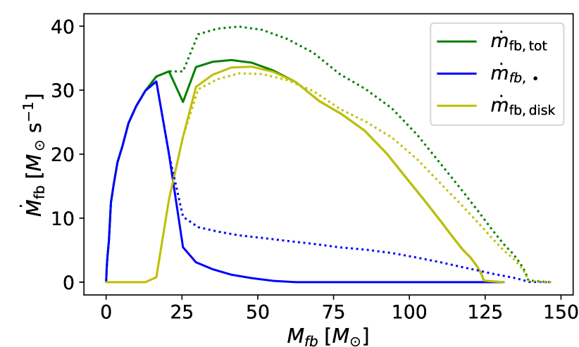
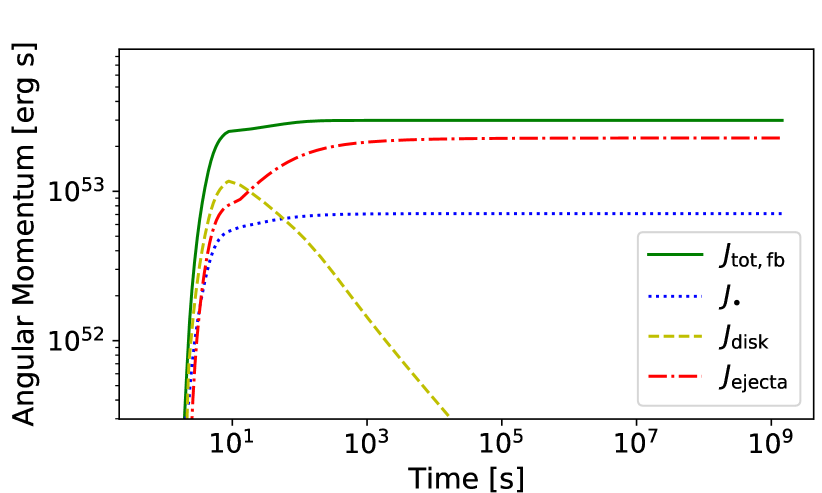
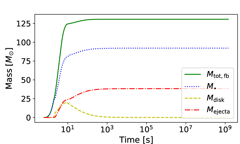
Figure 2: Collapse evolution for a representative stellar model 250.25 with typical rotation parameters $p=4.5$, $f_{\rm K}=0.3$ and $r_{\rm b}=1.5\times 10^{9}$ cm. Top: fallback rates $\dot{M}_{\rm fb}$ onto the BH (direct; blue), onto an accretion disk (yellow), and total (green), as a function of the total cumulative collapsed mass $M_{\rm fb}$. Dotted lines indicate the corresponding evolution when ignoring the effect of a jet. Center and bottom: evolution of angular momenta (center) and masses (bottom) as determined by Eqs. (9)–(14).

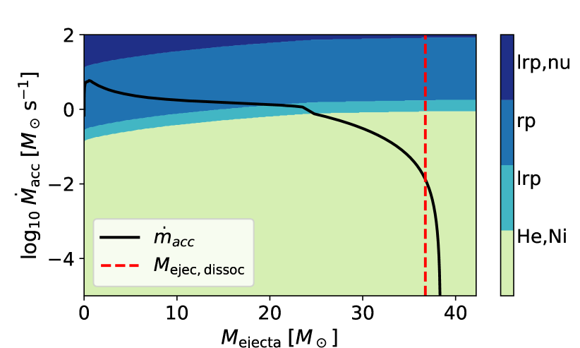
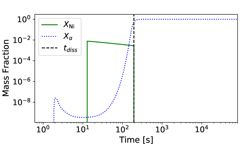
Figure 3: Top: accretion rate at which ejecta is being produced as a function of cumulative ejecta mass for model 250.25 with $p=4.5$, $f_{\rm kep}=0.3$, and $r_{\rm b}=1.5\times 10^{9}$ cm. The nucleosynthesis regimes according to Eq. (26) are color-coded. Bottom: corresponding mass fraction of ⁵⁶Ni synthesized in disk outflows and of ⁴He in the accretion disk. The vertical dashed line refers to the time $t_{\rm diss}$ at which only 50% of $\alpha$-particles are dissociated in the disk. For $t>t_{\rm diss}$ we ignore further ⁵⁶Ni production in the outflows.

Figure 2 illustrates the collapse evolution of model 250.25 with representative rotation parameters of $p=4.5$, $f_{\rm K}=0.3$, and $r_{\rm b}=1.5\times 10^{9}$ cm. Upon seed BH formation, the BH grows rapidly in mass and spin through low-angular momentum material at small radii directly falling into the seed BH before circularizing. Only after a few seconds and accretion of $\approx\!10\,M_{\odot}$ of the inner layers, first material starts to circularize outside the BH horizon to form an accretion disk (cf. Fig. 2, top and bottom panel), and initiate accretion onto the BH through a disk in addition to direct infall.

Direct fallback onto the BH subsides after the accretion of about $20\,M_{\odot}$ in this model (cf. Fig. 2, top panel) when a significant fraction of low angular momentum material residing in the polar region of the progenitor model has fallen into the BH. Further BH growth then proceeds almost entirely through disk accretion. This initial direct fallback episode partially clears up the polar regions for a relativistic jet to propagate through the outer stellar layers to eventually break out of the star and generate a long gamma-ray burst. Around the same time, a significant fallback rate onto the disk sets in (cf. Fig. 2, top panel) to establish a heavy $\sim\!15\,M_{\odot}$ accretion disk on a timescale of a few seconds (cf. Fig. 2, bottom panel). The disk accretion rate onto the BH, $\dot{m}_{\rm acc}$, quickly exceeds $\dot{M}_{\rm ign}$ and we assume that a relativistic jet forms. This removes the remaining low-angular momentum material in the polar regions and thus results in suppression of direct fallback onto the BH, which becomes negligible compared to disk fallback (cf. Fig. 2, top panel).

The top panel of Fig. 2 also shows that ignoring the effect of such a jet would lead to subdominant extended direct fallback of residual low-angular momentum material in polar regions onto the BH. While this does not have a direct impact on disk accretion, it has minor indirect consequences on nucleosynthesis in the disk winds due to its effect on the BH mass (cf. Eq. (26)). For somewhat larger values of $r_{\rm b}$, the situation changes and direct fallback onto the BH may extend to late times even in the presence of a jet, due to the overall lower angular momentum budget of the progenitor star outside the polar cone with opening angle $\theta_{\rm jet}$. For more extreme scenarios, fallback onto the disk may become close to non-existent.

As soon as the disk forms, most angular momentum resides in the disk rather than the BH in this model (cf. Fig. 2, center panel). The majority of this is being blown off in the ejecta, while a subdominant amount is transferred to the BH as disk matter gradually accretes through the ISCO onto the BH. For significantly larger values of $r_{b}$ this trend reverses, and most angular momentum is transferred to the BH rather than the ejecta as less material accretes through a disk.

The top panel of Fig. 3 shows the history of ejecta production in the model discussed above. Shown is the instantaneous accretion state $M_{\rm disk}/t_{\rm visc}$ of the disk as a function of the cumulative ejected wind mass, together with the nucleosynthesis regimes defined in Eq. (26). This evolution shows a ‘sweep’ through most nucleosynthesis regimes, typical of the models considered here. Nucleosynthesis regimes change during the evolution as a result of the BH mass growth and can be more dramatic in some cases than illustrated here. Outflows are first created in the regime of a main $r$-process with lanthanide production, during which the bulk of the wind ejecta is produced. The remaining $\approx 10\,M_{\odot}$ of ejecta originate in a regime that mostly ejects $\alpha$-particles and $\sim\!0.1\,M_{\odot}$ of ⁵⁶Ni. The bottom panel of Fig. 3 illustrates ⁵⁶Ni production in this regime. Shown are the mass fraction of ⁵⁶Ni produced in disk outflows according to Eq. (B2) as well as the mass fraction of $\alpha$-particles in the accretion disk according to Eq. (B6). The vertical dashed line indicates the dissociation time $t_{\rm diss}$ after which $<50\%$ of $\alpha$-particles are dissociated into individual nucleons in the accretion disk (Sec. 2.2, Appendix B). As a conservative estimate, for $t>t_{\rm diss}$, we ignore any further production of ⁵⁶Ni according to Eq. (B2) as the required free nucleons become unavailable. However, this represents only a slight correction in most cases, as by far the dominant amount of ⁵⁶Ni is typically produced before $t=t_{\rm diss}$.

2.3.2 Parameter Study of Massive Collapsars

Before systematically applying our model across the parameter space of massive collapsars, we first apply it to ‘ordinary’ collapsars of stars well below the PI mass gap, the results of which we describe in Appendix D. We use the progenitor models of Heger et al. (2000) as representative of typical stellar progenitors of canonical long GRBs (MacFadyen & Woosley, 1999). Our results for the nucleosynthesis yields of the disk outflows as a function of the parameters $\{f_{\rm K},r_{\rm b}\}$ which enter the progenitor angular momentum profile (Fig. 16), broadly agree with those previously presented in Siegel et al. (2019), though some quantitative differences arise due to our more detailed treatment of different regimes of BH accretion (see Appendix D for a discussion). Our low-mass collapsar models also exhibit BH accretion timescales and energetics of putative jet activity in agreement with long GRB observations. We can therefore claim a rough “calibration” of our model across the adopted parameter space of progenitor angular momentum properties, allowing for more confidence when extrapolating to the regime of more massive collapsars described below.

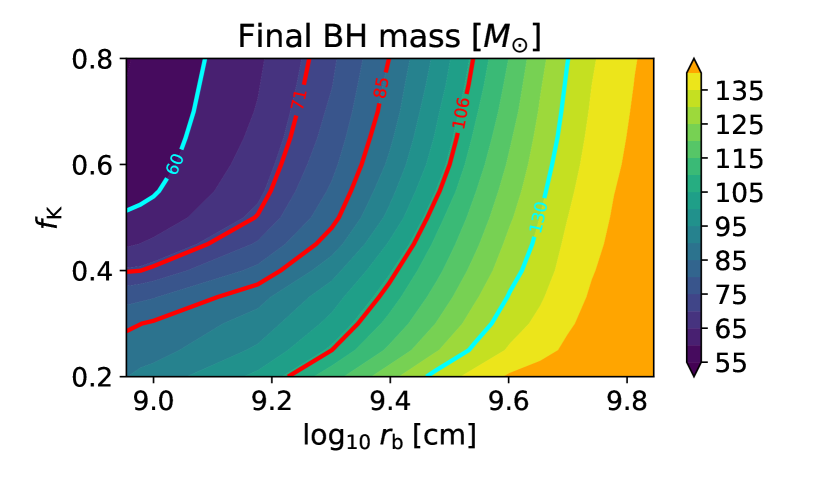
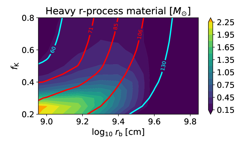
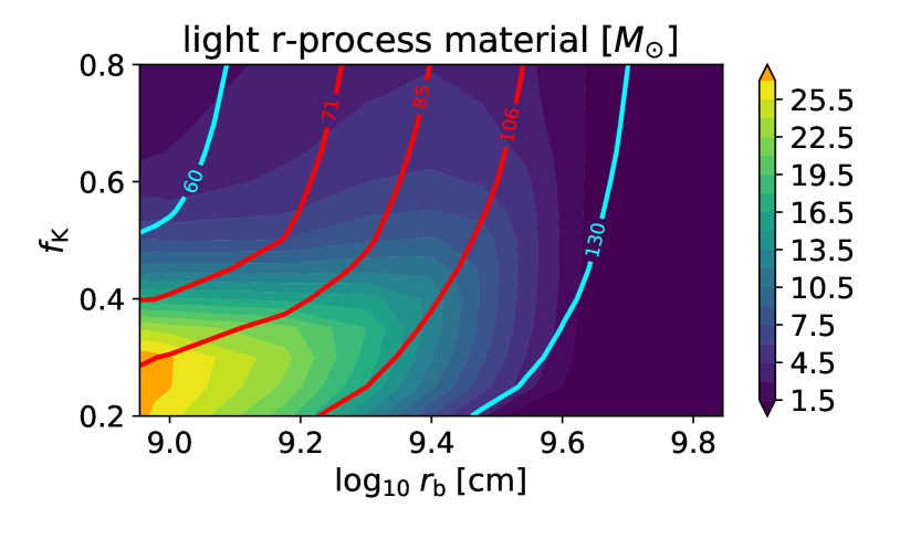
Figure 4: BH masses and disk wind ejecta properties across the parameter space of progenitor rotational profiles (envelope Keplerian fraction $f_{\rm K}$ and break radius $r_{\rm b}$; see Fig. 1, bottom panel) for model 250.25. Shown are the final BH mass (top), the total ejected mass in heavy ($A>136$) $r$-process elements including lanthanides (center top), light ($A<136$) $r$-process material (center bottom), and ⁵⁶Ni (bottom). Red contours indicate the inferred primary mass of GW190521, together with its 90% confidence limits ($85^{+21}_{-14}\,M_{\odot}$; Abbott et al. 2020). Cyan contours delineate final BH masses of 60 $M_{\odot}$ and 130 $M_{\odot}$, which approximately correspond to the lower and upper end of the PI mass gap.

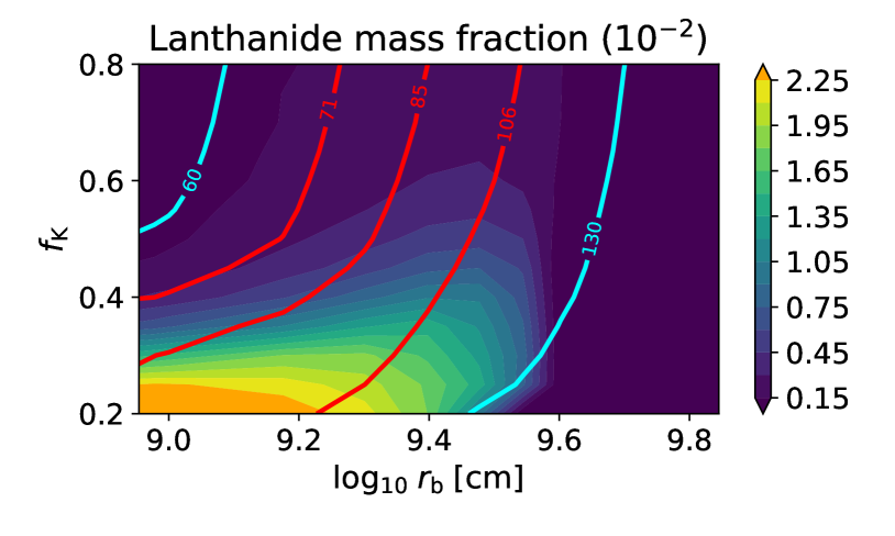
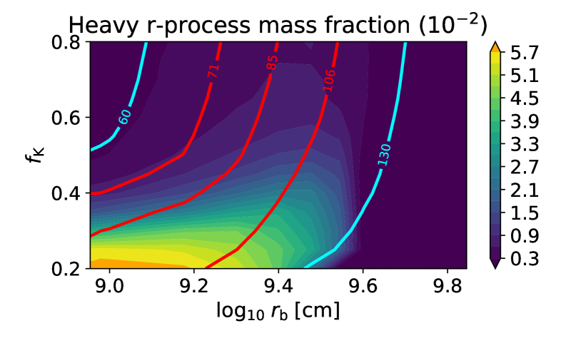
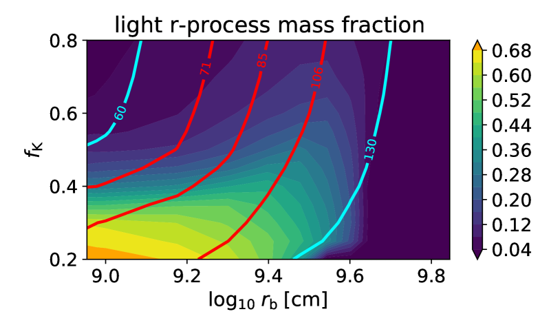
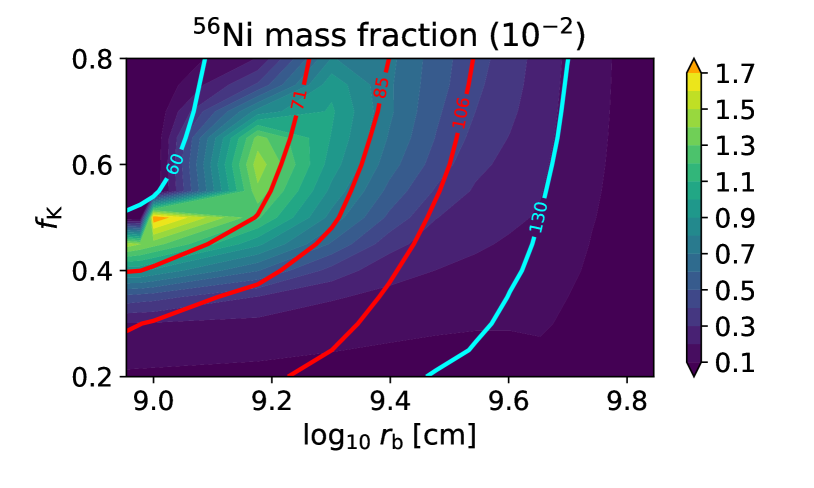
Figure 5: Scan of the parameter space for model 250.25. We show the mass fractions of lanthanides (top), light $r$-process elements ($A<136$; center), and of ⁵⁶Ni (bottom) in the ejecta, assuming full mixing of ejecta components. Red contours indicate the inferred primary mass of GW190521, together with its 90% confidence limits. Cyan contours delineate final BH masses of 60 $M_{\odot}$ and 130 $M_{\odot}$, which approximately correspond to the lower and upper end of the PI mass gap.

Figs. 4 and 18 summarize our results for the ejecta and GRB properties for model 250.25 as a representative example of a stellar model above the PI mass gap, in the parameter space $\{f_{\rm K},r_{\rm b}\}.$ The top panel of Fig. 4 shows that, even for a progenitor mass $M_{\star}=150\,M_{\odot}$ at the onset of collapse (that is, well above the PI mass gap), the final BH remnant can populate the entire mass gap between $\sim\!55\,M_{\odot}-130\,M_{\odot}$ (for typical parameter values), depending on the rotation profile at the onset of collapse. Labelled contours indicate the inferred primary mass of GW190521, together with its 90% confidence limits. We focus on this region of the parameter space in what follows, insofar that superKNe generated from such events probe BHs formed in the PI mass gap.

As in case of the low-mass collapsars (Appendix D), our results are not sensitive to the precise value of the power-law coefficient $p$, which we thus ignore in what follows. We find ubiquitous $r$-process production throughout the parameter space, ranging between $\sim 0.1-2.3\,M_{\odot}$ of heavy ($A>136$) $r$-process material including lanthanides and $\sim 1-29\,M_{\odot}$ of light ($A<136$) $r$-process elements. Additionally, between $\sim 0.05-1\,M_{\odot}$ of ⁵⁶Ni are synthesized in the ejecta.

Interestingly, the region of highest $r$-process production is well aligned with intermediate final BH masses in a range similar to the GW190521 confidence region (Sec. 5.3). For large $r_{\rm b}$ the outer stellar layers possess too little angular momentum to form massive accretion disks that give rise to copious $r$-process ejecta, as most material directly falls into the BH. On the other hand, for small values of $r_{\rm b}$ and high values of $f_{\rm K}$ massive disks form; however, high angular momentum leads to large disk radii $r_{\rm disk}$ and associated viscous timescales, such that the accretion rate drops below the required thresholds for $r$-process production for most of the accretion process. This occurs despite the presence of spiral modes in this regime, which tend to increase the accretion rate (Sec. 2.2). Most $r$-process material (both light and heavy) is synthesized for small values of both $r_{\rm b}$ and $f_{\rm K}$, which represents the optimal compromise between high angular momentum and sufficient compactness of the accretion disk. We discuss the possible contribution of massive collapsars to the long GRB population in Sec. 4.3.

For use in our subsequent light curve models (Sec. 3), we decompose the ejecta content of the collapsar models further into mass fractions of several constituents of interest. Assuming full mixing of all ejecta content (see also Sec. 3.1), we calculate the mass fraction $X_{\rm La}$ of lanthanides (atomic mass number $136\lesssim A\lesssim 176$) based on the amount of main $r$-process material, assuming the solar $r$-process abundance pattern (Arnould et al., 2007) motivated by the results of Siegel et al. (2019). A mass fraction $X_{\rm lrp}$ for light $r$-process elements is based on the combined mass fraction of light $r$-process material only plus the fraction of main $r$-process ejecta with $A<136$ when applying the solar $r$-process abundance pattern. Finally, we also compute the mass fraction $X_{\rm Ni}$ of ⁵⁶Ni. Results are depicted in Fig. 5. For concreteness, we select several models along iso-mass contours for the final BH mass within the GW190521 confidence region and report the corresponding ejecta parameters in Tab. 1.

Table 1: Ejecta parameters for select mass gap collapsar models with $p=4.5$ along contours of constant final BH mass (cf. Figs. 4 and 5).

model	$M_{\bullet}$	$M_{\rm ej}$	$r_{\rm b}$	$f_{\rm K}$	$X_{\rm La}$	$X_{\rm lrp}$	$X_{\rm Ni}$	$X_{\rm Ni}/X_{\rm rp}$
	($M_{\odot}$)	($M_{\odot}$)	($10^{9}$ cm)
250.25	106	27.24	1.94	0.25	0.020	0.59	0.0011	0.0018
	106	29.67	2.35	0.35	0.014	0.47	0.0020	0.0041
	106	30.51	2.67	0.45	0.008	0.36	0.0028	0.0075
	106	31.53	3.04	0.60	0.004	0.21	0.0039	0.0179
	85	45.57	1.20	0.35	0.012	0.47	0.0040	0.0079
	85	46.25	1.69	0.45	0.007	0.32	0.0059	0.0175
	85	47.20	1.96	0.55	0.005	0.22	0.0070	0.0303
	85	47.48	2.06	0.60	0.004	0.19	0.0072	0.0359
	71	58.06	1.19	0.50	0.004	0.19	0.0120	0.0601
	71	58.22	1.37	0.55	0.003	0.16	0.0094	0.0562
	71	58.00	1.50	0.60	0.003	0.13	0.0058	0.0417
	71	59.78	1.53	0.65	0.002	0.11	0.0121	0.1035
200.25	106	11.41	2.14	0.25	0.011	0.42	0.0013	0.0029
	106	13.87	2.59	0.35	0.008	0.34	0.0019	0.0054
	85	28.77	1.32	0.35	0.016	0.53	0.0026	0.0046
	85	29.74	1.59	0.45	0.010	0.39	0.0040	0.0096
	71	40.93	1.07	0.50	0.007	0.29	0.0079	0.0254
	71	40.64	1.21	0.55	0.006	0.25	0.0083	0.0308

3 Super-Kilonova Emission

As the disk outflows expand away from the BH, the ejecta shell they form eventually gives rise to optical/infrared emission powered by radioactive decay (the “superKN”).

3.1 Analytic Estimates

We begin with analytic estimates of the superKN properties. The total ejecta mass $M_{\rm ej}$ is comprised of up to three main components: (1) radioactive $r$-process nuclei, mass fraction $X_{\rm rp}$; (2) radioactive ⁵⁶Ni, $X_{\rm Ni}$; (3) non-radioactive ⁴He, $X_{\rm He}=1-X_{\rm rp}-X_{\rm Ni}$ (also a placeholder for other non-radioactive elements). Typical values for our fiducial models (Sec. 2.3) are $M_{\rm ej}\sim 10-60M_{\odot}$, $X_{\rm rp}\sim 0.1-0.5$, $X_{\rm Ni}\sim 10^{-3}-10^{-2}$ ($M_{\rm Ni}\sim 10^{-2}-0.5M_{\odot}$). As described in the previous section, the total $r$-process mass fraction can be further subdivided into that of light $r$-process nuclei $X_{\rm lrb}$ and of lanthanides $X_{\rm La}$. For simplicity, throughout this section we assume the ejecta are mixed homogeneously into a single approximately spherical shell. Physically, such mixing could result from hydrodynamic instabilities that develop between different components of the radial and temporally-dependent disk winds and or due to its interaction with the GRB jet (e.g., Gottlieb et al. 2021).

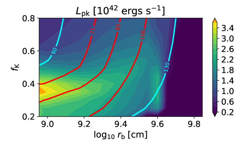
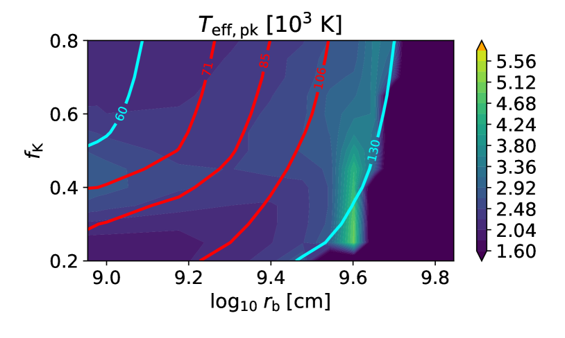
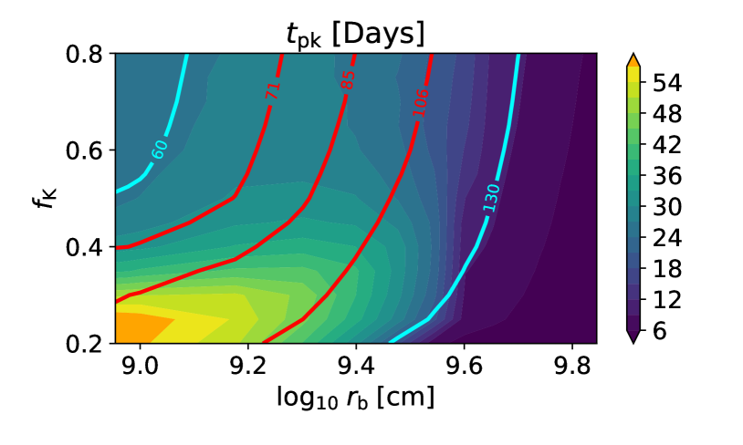
Figure 6: Analytic light curve estimates across the parameter space for model 250.25. Shown are the peak luminosity (top), peak effective temperature (center), and peak timescale (bottom). Red contours indicate the inferred primary mass of GW190521, together with its 90% confidence limits. Cyan contours delineate final BH masses of 60 $M_{\odot}$ and 130 $M_{\odot}$, which approximately correspond to the lower and upper end of the PI mass gap.

The light curve will peak roughly when the expansion timescale equals the photon diffusion timescale (e.g., Arnett 1982),

$$t_{\rm pk} \approx \left(\frac{M_{\rm ej}\kappa}{4\pi v_{\rm ej}c}\right)^{1/2}$$

$$\approx 108\,{\rm d}\left(\frac{M_{\rm ej}}{50M_{\odot}}\right)^{1/2}\left(\frac{v_{\rm ej}}{0.1c}\right)^{-1/2}\left(\frac{\kappa}{1{\rm cm^{2}\,g^{-1}}}\right)^{1/2},$$

where $v_{\rm ej}$ is the average ejecta velocity. The effective gray opacity $\kappa$ varies in kilonovae from $\lesssim 1$ cm² g^-1 for ejecta dominated by light $r$-process species, to $\sim 10-30$ cm² g^-1 for ejecta containing a sizable quantity of lanthanide atoms and ions (e.g., Kasen et al. 2013; Tanaka et al. 2020). However, $\kappa$ will be smaller than these estimates in the superKN case due to the large mass fraction of light elements, $X_{\rm He}\sim 0.5-0.9$, which contribute negligibly to the opacity. For our analytical estimates below, we linearly interpolate $\kappa$ between 0.03 cm² g^-1(at $X_{\rm La}=10^{-4}$) and 3 cm² g^-1 (at $X_{\rm La}\geq 0.2$), which we find results in reasonable agreement with the detailed radiation transport calculations present in Sec. 3.2.

The peak luminosity and effective temperature can also be estimated using analytic formulae (e.g., Metzger 2019),

$$L_{\rm pk} \approx 4\times 10^{41}{\rm erg\,s^{-1}}\left(\frac{X_{\rm rp}}{0.2}\right)$$

$$\times\left(\frac{M_{\rm ej}}{50M_{\odot}}\right)^{0.35}\left(\frac{v_{\rm ej}}{0.1c}\right)^{0.65}\left(\frac{\kappa}{{\rm cm^{2}\,g^{-1}}}\right)^{-0.65},$$

$$T_{\rm eff,pk} \approx 900\,{\rm K}\left(\frac{X_{\rm rp}}{0.2}\right)^{0.25}$$

$$\times\left(\frac{M_{\rm ej}}{50M_{\odot}}\right)^{-0.16}\left(\frac{v_{\rm ej}}{0.1c}\right)^{0.41}\left(\frac{\kappa}{{\rm cm^{2}\,g^{-1}}}\right)^{-0.41},$$

where we have used the radioactive heating rate of $r$-process nuclei from Metzger et al. (2010) with an assumed thermalization efficiency of 50%. Near peak light $t\sim t_{\rm pk}\sim$ 100 d, the specific radioactive heating rate of ⁵⁶Ni is $\sim 10-30$ times higher than that of $r$-process elements (e.g., Siegel et al. 2019). Given values $X_{\rm Ni}/X_{\rm rp}\sim 0.01-0.05$ for most of our disk outflow models, $L_{\rm pk}$ is moderately underestimated by Eq. (3.1), which neglects ⁵⁶Ni heating.

Fig. 6 shows the predicted peak timescale, luminosity, and effective temperature of the superKN emission in the parameter space $\{f_{\rm K},r_{\rm b}\}$ for the fiducial model 250.25. For the same parameters which generate remnant BHs with masses in the PI gap, we predict peak luminosities $L_{\rm pk}\sim 10^{42}$ erg s^-1 and characteristic durations of months. Though similar to other types of SNe in duration, superKNe are characterized by significantly cooler emission ($T_{\rm eff}\approx 1000$ K), as confirmed by radiative transfer calculations presented in the next section.

3.2 SuperKN Light Curves and Spectra

Table 2: SuperKN Light Curve Models and Survey Detection Rates

Model	$M_{\rm ej}$	$v_{\rm ej}$	$M_{\rm Ni}$	$M_{\rm lrp}$	$X_{\rm La}$	$R_{\rm Rubin}^{(a)}$	$R_{\rm Roman}^{(b)}$
	($M_{\odot}$)	($c$)	($M_{\odot}$)	($M_{\odot}$)	($10^{-3}$)	(yr-1)	(yr-1)
a	8.6	0.1	0.019	0.83	1.4	0.01	0.02
b	31.0	0.1	0.012	8.28	17.0	0.03	0.4
c	35.6	0.1	0.087	23.2	4.0	0.1	2
d	50.0	0.1	0.53	9.59	0.53	0.1	4
e	60.0	0.1	0.0	5.6	0.17	0.2	0.01

${}^{(a)},^{(b)}$Detection rates per year by Rubin Observatory and Roman, respectively for an assumed $z=0$ superKN rate of 10 Gpc^-3 yr^-1 (see Sec. 4.2 for details).

3.2.1 Model Selection and Parameters

To elaborate on the estimates of §3.1, we carried out detailed radiation transport simulations for five ejecta models whose properties ($M_{\rm ej}$, $M_{\rm Ni}$, $M_{\rm lrp}$, and $M_{\rm La}$) span the space defined by the subset of simulations that produced BHs within the mass gap ($60\lesssim M_{\bullet}/M_{\odot}\lesssim 130$), i.e., models that fall between the two cyan contours of Fig. 5. (See also Woosley 2017; Farmer et al. 2019; Renzo et al. 2020b; Farmer et al. 2020; Costa et al. 2021; Mehta et al. 2021). The parameters of the mass gap models are largely confined to a plane in $M_{\rm ej}$-$M_{\rm Ni}$-$M_{\rm lrp}$-$M_{\rm La}$ space, making it straightforward to select a handful of characteristic parameters from the full set. We used the KMeans routine of sklearn (Pedregosa et al., 2011) to divide our models into four clusters, and adopted the positions of the cluster centers as four representative super-kilonova models. However, a small fraction of the mass-gap models occupy a distinct region of the parameter space, having large $M_{\rm ej}$, but little to no nucleosynthetic products heavier than He. Since these models were not captured by our clusters, we added a fifth model to explore the edge case of a high-mass, nickel-free outflow. Our five models are listed in Tab. 2.

We performed for the models of Tab. 2 one-dimensional radiation transport calculations carried out with Monte Carlo radiation transport code Sedona (Kasen et al., 2006, in prep.). We adopted for each model a density profile such that the mass external to the velocity coordinate $v$ follows a power-law,

$$M_{>v}\propto\left(\frac{v}{v_{\rm min}}\right)^{-\alpha},\>\>v\geq v_{\rm min}.$$ (31)

Above, the minimum ejecta velocity $v_{\rm min}$ is determined by the characteristic velocity $v_{\rm ej}=(2E_{\rm kin}/M_{\rm ej})^{1/2}$ (with $E_{\rm kin}$ the ejecta kinetic energy), and the choice of power-law index $\alpha$,

$$v_{\rm min}=\left(\frac{\alpha-2}{\alpha}\right)^{1/2}v_{\rm ej}.$$ (32)

We take $\alpha=2.5$ and $v_{\rm ej}=0.1c$ for all models, consistent with predictions of accretion disk outflow velocities (e.g. Fernández et al., 2015; Siegel et al., 2019).

The opacity of the outflowing gas, and therefore the nature of the transients’ electromagnetic emission, is sensitive to the abundance pattern in the ejecta. Specifically, lanthanides and actinides, and to a lesser extent elements in the d-block of the periodic table, contribute a high opacity, while the opacities of s- and p- block elements is significantly lower (Kasen et al., 2013; Tanaka et al., 2020).

In this work, we predict the synthesis of helium, ${}^{56}\mathrm{Ni}$, and light and heavy r-process material, but do not carry out detailed nucleosynthesis calculations, e.g. by post-processing fluid trajectories. The composition of each model is then solely a function of its $M_{\rm ej}$, $M_{\rm Ni}$, $M_{\rm lrp}$, and $X_{\rm La}$. We assume that heavy ($A>136$) r-process material is 41% lanthanides and actinides by mass, equal to the solar value of $M_{\rm La}/M_{\rm A>136}$. The remainder is split between d-block and s/p-block elements (54% and 5% by mass, respectively). For light r-process material, $X_{\rm La}=0$. We estimated it comprises 95% (5%) d-block (s-/p-block) elements by mass.

The composition adopted for our radiation transport models is limited by both our imperfect knowledge of the details of nucleosynthesis and incomplete atomic data of the sort necessary to calculate photon opacities in the ejecta. Lanthanide and actinide mass ($M_{\rm La}$) is divided among lanthanide elements following the solar pattern, with one adjustment: because the required atomic data is not available for atomic number Z=71, we redistribute the solar mass fraction of Z=71 to Z=70.

Atomic data is also unavailable for most of the d-block elements produced by r-process (whether heavy or light). We thus distribute d-block mass evenly among elements with $Z=21-28$ (excluding $Z=23$ for lack of data), artificially increasing the mass numbers to $A\sim 90$ to avoid overestimating the ion number density. All r-process s- and p-block material is modeled by the low-opacity filler Ca ($Z=20$). ⁴He and ${}^{56}\mathrm{Ni}$ (as well as its daughter products ${}^{56}\mathrm{Co}$ and ${}^{56}\mathrm{Fe}$) are straightforward to incorporate into the composition.

Our radiation transport simulations include radioactivity from both the ${}^{56}\mathrm{Ni}$ decay chain and from the r-process. We explicitly track energy loss by $\gamma$-rays from ${}^{56}\mathrm{Ni}$ and ${}^{56}\mathrm{Co}$, and assume that positrons from ${}^{56}\mathrm{Co}$ decay thermalize immediately upon production. We model r-process radioactivity using the results of Lippuner & Roberts (2015) for an outflow with $(Y_{\rm e},s_{\rm B},\tau_{\rm exp})=(0.13,32k_{\rm B},0.84\;\text{ms})$, with $s_{\rm B}$ the initial entropy per baryon and $\tau_{\rm exp}$ the expansion timescale. To account for thermalization, we adjust the absolute radioactive heating rate following the analytic prescription of Barnes et al. (2016).

3.2.2 Radiation Transport Results

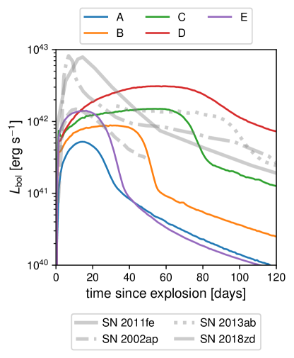
Figure 7: The bolometric light curves of the models in Tab. 2, compared to prototypical SNe 2011fe (Type Ia), 2002ap (Type Ic-bl), 2013ab (Type II-p), and 2018zd (electron-capture). The superKN light curves are dimmer than SNe Ia, but at some epochs can approximate the light curves of SNe Type Ic-bl and Type IIp.

The bolometric light curves of models A through E are presented in Fig. 7. For comparison, we also show the light curves of typical SNe of various subtypes: Type Ia SN 2011fe (Tsvetkov et al., 2013), Type Ic-bl SN 2002ap (Tomita et al., 2006), Type IIp SN 2013ab (Bose et al., 2015), and the electron-capture SN 2018dz (Hiramatsu et al., 2021) .

The superKN light curves exhibit considerable diversity, which is not surprising given the large ranges of ejecta and radioactive masses these systems may produce. As would be expected from simple Arnett-style (Arnett, 1982) arguments, higher masses are generally associated with longer light-curve durations. This can be seen in the progression from model A to model D.

However, as model E demonstrates, the shape of the light curve also depends on the presence of ${}^{56}\mathrm{Ni}$ in the ejecta. While the mass of r-process material burned in superKN outflows greatly exceeds that of ${}^{56}\mathrm{Ni}$, the energy generated by the ${}^{56}\mathrm{Ni}$ decay chain, per unit mass, exceeds that of r-process decay by orders of magnitude (e.g., Metzger et al. 2010; Siegel et al. 2019). When ${}^{56}\mathrm{Ni}$ is present, it can be the main source of radiation energy for the transient. As a result of the long half-life of the ${}^{56}\mathrm{Ni}$ daughter ${}^{56}\mathrm{Co}$ ($\tau_{1/2}^{\rm Co}\approx 77$ days), the energy generation rate for ${}^{56}\mathrm{Ni}$-producing systems is declining slowly just around the time the light curves reach their maxima. The effect is a more extended light curve (see Khatami & Kasen 2019 and Barnes et al. 2021 for more detailed discussions).

Model E, which produces no ${}^{56}\mathrm{Ni}$, has a relatively short (${\sim}$month) duration, despite its high mass ($M_{\rm ej}=60M_{\odot})$, owing to the steep decline of the r-process radioactivity that is its only source of energy. The qualitative difference between models that burn even small amounts of ${}^{56}\mathrm{Ni}$ and models that burn none points to the importance of a careful treatment of nucleosynthesis in disk outflows.

As is apparent from Fig. 7, the diversity of superKN light curves allows them to mimic other types of SNe. While superKNe do not produce sufficient ${}^{56}\mathrm{Ni}$ to approach the luminosity of SNe Ia, they can, at various epochs, mimic the bolometric light curves of SNe Ic-bl, SNe IIp as well as electron-capture SNe. However, the high opacity of the r-process-enriched ejecta pushes the superKN emission to redder wavelengths than what is observed for other classes of SNe. This is illustrated in Fig. 8, which shows the normalized spectra for models A through E at bolometric peak.

Unlike other types of SNe, most of the superKN flux emerges at near- and even mid-infrared wavelengths. This is likely due to a combination of lower radioactive heating per unit ejecta mass, as well as the high opacity from r-process elements (particularly lanthanides and actinides) and the high $M_{\rm ej}$, which work in concert to increase the optical depth across the ejecta and push the photosphere out to the exterior where temperatures are cooler.

A second distinguishing feature of superKNe is their broad absorption features. These are a product of our assumed ejecta velocities ($v_{\rm ej}=0.1c$), which are higher than what is inferred for all supernova other than the hyper-energetic SNe Ic-bl. And while SNe Ic-bl produce spectra with similarly wide absorption features, in the case of Ic-bl these features are found at much bluer (4000 Å$\lesssim\lambda\lesssim 8000$ Å) wavelengths. Thus, despite their bolometric similarities, superKNe are spectroscopically unique among SNe.

The peak photospheric temperatures of superKNe $\sim 1000$ K are also similar to those required for solid condensation, suggesting the possibility of dust formation in the ejecta (e.g., Takami et al. 2014; Gall et al. 2017). Insofar as the optical/NIR opacity of ${\sim}\mu$m sized dust is roughly comparable to that of lanthanide-enriched ejecta, dust formation would not qualitatively impact the appearance of the transient. However, this does imply potential degeneracy between the photometric signatures of superKNe and other dust-enshrouded explosions unrelated to $r$-process production, including stellar mergers (e.g., Kasliwal et al. 2017). This degeneracy with dusty transients can generally be broken by the predicted broad spectral features of superKNe $(v_{\rm ej}\sim 0.1c$).

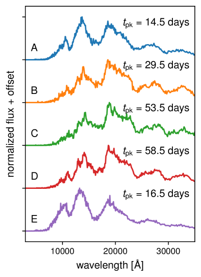
Figure 8: The flux per unit wavelength at bolometric peak for each of the five models defined in Tab. 2. All spectra have broad absorption features consistent with a high-velocity outflow, and a low-temperature, pseudo-black body spectrum, consistent with a high-opacity composition. These spectra distinguish superKNe from other classes of SNe, which are much bluer, and from other dust-enshrouded explosions, in which broad absorption features are absent.

4 Discovery Prospects

In this section we explore the discovery prospects of superKNe with future optical/infrared transient surveys and via late-time infrared follow-up observations of energetic long GRBs. We then discuss how superKN emission could be enhanced by circumstellar interaction for collapsars embedded in AGN disks.

4.1 Volumetric Rates

We begin by estimating the volumetric rate of superKNe. One approach is to scale from the observed rates of ordinary collapsars. The local (redshift $z\simeq 0$) volumetric rate of classical long GRBs is $\approx 0.6-2$ Gpc^-3yr^-1 (Wanderman & Piran, 2010), which for an assumed gamma-ray beaming fraction $f_{\rm b}=0.006$ (Goldstein et al., 2016), corresponds to a total collapsar rate of $\approx 100-300$ Gpc^-3 yr^-1. Under the assumption that ordinary collapsars originate from stars of initial mass $M_{\rm ZAMS}\gtrsim 40M_{\odot}$, then the more massive stars $M_{\rm ZAMS}\gtrsim 250M_{\odot}$ which generate helium core masses above the PI mass gap ($M_{\mathrm{BH}}\gtrsim 130M_{\odot}$) will be less common by at least a factor $\sim(40/250)^{\alpha-1}\sim 0.1-0.3$ for an initial-mass function (IMF) $dN_{\star}/dM_{\star}\propto M_{\star}^{-\alpha}$, where we consider values for the power-law index between $\alpha=2.35$ for a Salpeter IMF and a shallower value $\alpha\approx 1.8$ (Schneider et al. 2018). This optimistically assumes that (i) stars that massive exist (e.g., de Koter et al., 1997; Crowther et al., 2016), and that (ii) these can form helium cores such that $M_{\mathrm{He}}\simeq M_{\mathrm{ZAMS}}$, for instance because of rotational mixing (e.g., Maeder & Meynet, 2000; Marchant et al., 2016; de Mink & Mandel, 2016) or continuous accretion of gas (e.g., Jermyn et al., 2021; Dittmann et al., 2021). Various processes act to remove mass from a massive star during its evolution, and generally the more massive the star, the larger its mass loss rate. Some of these mechanisms (e.g., continuum-driven stellar winds and eruptive mass loss phenomena, see also Renzo et al. 2020a) might occur even at low metallicity.

With the above estimate and caveats, we obtain an optimistic maximum local rate of superKNe from massive collapsars of $\sim 10-100$ Gpc^-3 yr^-1. On the other hand, the long GRB rate increases with redshift in rough proportion to the cosmic star-formation rate (SFR $\propto(1+z)^{3.4}$ for $z\lesssim 1$; e.g., Yüksel et al. 2008) and hence the maximum rate of superKNe is larger at redshift $z\gtrsim 1$ by a factor $\sim 10$ than at $z\simeq 0$, corresponding to a maximum superKN rate of $\sim 100-1000$ Gpc^-3 yr^-1 at $z\gtrsim 1$.

The superKN rate question can be approached from another perspective: What is the minimum birth-rate of BHs in the PI mass gap to explain GW190521-like merger events (Sec. 5.3) via the massive collapsar channel? The rate of GW190521-like mergers at $z\simeq 0$ was estimated by LIGO/Virgo to be $\sim 0.5-1$ Gpc^-3 yr^-1 (Abbott et al., 2020). This rate is smaller than the maximum superKN rate estimated above, consistent with only a small fraction of BHs formed through this channel ending up in tight binaries that merge due to gravitational waves at $z\approx 0$.

4.2 Discovery with Optical/Infrared Surveys

We now evaluate the prospects for discovering superKNe with impending wide-field optical/infrared surveys.

First, we explore the expected observable rates within the Legacy Survey of Space and Time (LSST) conducted with the Vera Rubin Observatory. LSST is currently set to commence in early 2024 and will explore the southern sky in optical wavelengths to a $5\sigma$ stacked nightly visit depth of $\sim 24$ mag. We inject the set of SEDONA light curves of models described in Tab. 2 into the publicly available LSST operations simulator, OpSim (Delgado & Reuter, 2016). We use the most recent baseline scheduler (baseline v1.7) to calculate LSST pointings, limiting magnitudes, and expected sky noise across a full simulated 10 year survey in $ugrizY$ bands. We additionally apply dust reddening following the dust maps of Schlegel et al. (1998). For each model, we inject a superKN randomly 300 times within the full LSST simulation (including both the wide-fast-deep survey and deep-drilling fields) at redshift bins of 0.01.

We find that superKNe discovered with LSST are confined to the local universe, with $z<0.1$. Assuming that the superKN rate traces star-formation with a local rate of 10 Gpc^-3yr^-1, we expect LSST to discover $\sim 0-0.2$ superKNe annually, resulting in up to $2$ events over its 10-year nominal duration. We note that the larger the ejecta masses (i.e., Models b and e) the most likely the detection with LSST.

Given the expected red colors of the superKN emission (Fig. 8), we additionally explore the possibility of discovering superKN with the Nancy Grace Roman Space Telescope, expected to launch in the mid 2020s. Although not fully defined, Roman expects to conduct a $\sim 5$ year, 10 deg² SN survey, primarily targeted at Type Ia SNe for cosmological distance measurements. We assume a survey cadence of 30 days and single-visit, stacked $5\sigma$ depth of 27th magnitude, corresponding to roughly an hour of integration time (in F158 band). We inject the same set of models using the Roman F062, F158 and F184 filters, corresponding to central wavelengths of 0.62, 1.58 and 1.83 $\mu$m, respectively. We assume observations are taken in each filter at the same epoch, and consider superKNe with three or more $3\sigma$ detections to be detectable. Assuming the Roman wide-field survey footprint is chosen to minimize galactic dust, we do not account for any galactic reddening.

We find that Roman is most sensitive to models with the largest Lanthanide fractions. Assuming that the superKN rate traces star-formation with a local rate of 10 Gpc^-3yr^-1, we expect a 5 year Roman survey as described would find roughly 1–20 superKNe, most favoring the Lanthanide-rich Model B. These superKNe will be observable out to a redshift of $z\sim 0.9$. We note that longer cadences significantly decrease the number of superKN detections possible with Roman, at least within the 3-detection discovery criterion we have adopted.

4.3 Energetic Long GRB Accompanied by SuperKNe

SuperKNe could also be detected following a subset of long GRBs. Figure 18 summarizes the GRB properties for our fiducial massive collapsar model 250.25. We find accretion timescales comparable to those of ordinary collapsars from lower mass progenitor stars (Appendix D). These mass gap collapsars are therefore candidates for contributing to the observed population of long GRBs, except that they may be a factor of $\sim\!10$ times more luminous and energetic than typical GRBs if the gamma-ray luminosity tracks the BH accreted mass. Furthermore, if the fraction of massive stars above the PI mass gap which form or evolve into collapsar progenitors is greater at lower metallicity, this could imprint itself on the redshift evolution of the long GRB luminosity function (for which there is claimed evidence; Petrosian et al. 2015; Sun et al. 2015; Pescalli et al. 2016).

In the local universe, long GRBs with supernovae are commonly accompanied with the luminous hyper-energetic Type Ic SNe with broad lines (Ic-BL; e.g., Woosley & Bloom 2006; Japelj et al. 2018; Modjaz et al. 2020). The superKN transients we predict from the birth of more massive BHs are of comparable or moderately lower peak luminosities than ordinary collapsar SNe (e.g., Cano 2016) but significantly redder (Figs. 7, 8). Luminous optical SNe have been ruled out to accompany a few nominally long duration GRBs (Fynbo et al. 2006; Gehrels et al. 2006). One of these events, GRB 060614, was found to exhibit a red excess which Jin et al. (2015) interpreted as a kilonova. However, the luminosity and timescale of the excess could also be consistent with superKN emission from a massive collapsar of the type described here. We encourage future deep infrared follow-up observations of energetic long GRB with Roman or JWST on timescales of weeks to months after the burst to search for infrared superKN emission.

4.4 SuperKNe Embedded in AGN Disks

The optical emission from superKNe could be significantly enhanced by circumstellar interaction if they are embedded in a gas-rich environment.

Graham et al. (2020) reported a candidate optical wavelength counterpart to GW190521 in the form of a flare from an active galactic nucleus (AGN). The flare reached a peak luminosity $L_{\rm pk}\sim 10^{45}$ erg s^-1 in excess of the nominal level of AGN emission and lasted a timescale $t_{\rm pk}\sim 50$ days, over which it radiated a total energy of $E_{\rm rad}\sim 10^{51}$ erg. Shibata et al. (2021) propose a scenario for GW190521 as a massive stellar core collapse generating a single BH and a massive accretion disk $\gtrsim 10-50M_{\odot}$ rather than a binary BH merger. Although our results in Secs. 5.2 and 5.3 challenge this interpretation, our present work shows that a prediction of this scenario is a superKN counterpart with $M_{\rm ej}\sim 3-20M_{\odot}$ and $v_{\rm ej}\sim 0.1$ c. Though the predicted peak timescale, $t_{\rm pk}\sim 50$ days (Eq. 3.1), of the superKNe emission roughly agrees with that observed by Graham et al. (2020), the luminosity powered by radioactivity $\sim 10^{42}$ erg s^-1 (Fig. 7) is too small to explain the observations by several orders of magnitude.

This problem could be alleviated if the collapsing star is embedded in a dense gaseous AGN disk (e.g., Jermyn et al. 2021; Dittmann et al. 2021). If the density of the AGN disk at the star location is sufficiently high, $\rho\gtrsim 10^{-15}\,\mathrm{g\ cm^{-3}}$, runaway accretion of mass might help building up very massive and fast rotating helium cores. The mass accretion might be interrupted as the AGN turns off (on a few Myr timescale), and depending on the balance between mass loss processes and the previous accretion phase one might obtain a superKN progenitor. At its collapse, the shock-mediated collision between the superKN ejecta and the surrounding disk material could power a more luminous optical signal than from radioactive decay alone, akin to interaction-powered super-luminous SNe (e.g., Smith et al. 2007).

Given the large kinetic energy of the superKN ejecta, $E_{\rm kin}\sim M_{\rm ej}v_{\rm ej}^{2}/2\sim 1-5\times 10^{53}$ erg, the Graham et al. (2020) transient could be powered by tapping into only $\sim 1\%$ of $E_{\rm kin}$ by shock deceleration. Insofar as such luminous shocks are radiative and momentum-conserving, the swept-up gaseous mass in the AGN disk required to dissipate $E_{\rm rad}\sim 10^{51}$ erg is only $M_{\rm sw}\sim(E_{\rm rad}/E_{\rm kin})M_{\rm ej}\sim 0.1-1M_{\odot}$. Treating the swept-up material as being approximately spherical and expanding at $\sim v_{\rm ej}$, the optical diffusion time through $M_{\rm sw}$ is (Eq. 3.1),

$$t_{\rm pk,min}\approx 5\,{\rm d}\left(\frac{M_{\rm sw}}{0.3M_{\odot}}\right)^{\frac{1}{2}}\mskip-5.0mu\left(\frac{v_{\rm ej}}{0.1c}\right)^{-\frac{1}{2}}\mskip-5.0mu\left(\frac{\kappa}{0.3\,{\rm cm^{2}\,g^{-1}}}\right)^{\frac{1}{2}},$$ (33)

where $\kappa$ is now normalized to a value more appropriate to AGN disk material. Insofar that $t_{\rm pk,min}$ is significantly shorter than the observed $\sim 50$ d rise time of the Graham et al. (2020) counterpart, this implies the rise of the putative counterpart would instead need to be limited by photon diffusion through the unshocked external AGN disk material (e.g., Graham et al. 2020; Perna et al. 2021).

A bigger challenge for this scenario is the typically much closer source distance for GW190521 that would be predicted if this resulted from a self-gravitating collapsar disk instead of a binary BH merger (redshift $z\lesssim 0.05$; Sec. 5.2), compared to that of the AGN identified by Graham et al. (2020) at redshift $z=0.438$.

5 Other Observable Implications

5.1 Luminous Slow Radio Transients

In addition to their prompt optical/IR signal, superKNe produce synchrotron radio emission as the ejecta decelerates by driving a shock into the circumburst medium (e.g., Nakar & Piran 2011; Metzger & Bower 2014). This emission can be particularly luminous because the kinetic energy of the superKN ejecta $E_{\rm kin}\approx 1-5\times 10^{53}$ erg can be one to two orders of magnitude higher than those of ordinary collapsar SNe.

The radio transient rises on the timescale required for the ejecta to sweep up a mass comparable to their own,

$$t_{\rm radio}\approx 200\,{\rm yr}\left(\frac{E_{\rm kin}}{5\times 10^{53}\,\rm erg}\right)^{\frac{1}{3}}\mskip-5.0mu\left(\frac{v_{\rm ej}}{0.1c}\right)^{-\frac{5}{3}}\mskip-5.0mu\left(\frac{n}{\rm 1\,cm^{-3}}\right)^{-\frac{1}{3}},$$ (34)

where $n$ is the particle density of the external medium. The peak luminosity at a frequency $\nu=$ 1 GHz can be estimated as (e.g., Nakar & Piran 2011)

$$\nu L_{\nu} \approx 5\times 10^{39}\,{\rm erg\,s^{-1}}\left(\frac{E_{\rm kin}}{5\times 10^{53}\,\rm erg}\right)\left(\frac{v_{\rm ej}}{0.1c}\right)^{2.3}$$ (35)

$$\times\left(\frac{n}{\rm 1\,cm^{-3}}\right)^{0.83}\left(\frac{\epsilon_{e}}{0.1}\right)^{1.3}\left(\frac{\epsilon_{B}}{0.01}\right)$$

where the fraction of the shock energy placed into relativistic electrons $\epsilon_{e}$ and magnetic fields $\epsilon_{B}$ are normalized to characteristic values, respectively, and we have assumed a power-law index $p=2.3$ for the energy distribution of the shock accelerated electrons, $dN/dE\propto E^{-p}$.

For characteristic circumstellar densities $n\sim 0.1-10$ cm^-3 the peak radio luminosity is comparable to that of rare energetic transients, such as those from binary neutron star mergers that generate stable magnetar remnants (e.g., Metzger & Bower 2014; Schroeder et al. 2020). However, the predicted timescale of the radio evolution of decades to centuries is much longer in the superKN case due to the large ejecta mass. This slow evolution makes it challenging to uniquely associate the radio source with a known GRB or gravitational wave event, or to even identify it as a transient in radio time-domain surveys (e.g., Metzger et al. 2015). We note that luminous radio point sources are in fact common in the types of dwarf galaxies which host collapsars (e.g., Eftekhari et al. 2020). Ofek (2017) place an upper limit on the local volumetric density of persistent radio sources in dwarf galaxies of luminosity $\gtrsim 3\times 10^{38}$ erg s^-1 of $\mathcal{N}\lesssim 5\times 10^{4}$ Gpc^-3. Assuming the superKN radio emission remains above this luminosity threshold for a time $t_{\rm det}\sim 10t_{\rm radio}\sim 10^{3}$ yr, this constrains the local rate of superKNe to obey $\lesssim 10-100$ Gpc^-3 yr^-1, consistent with the estimates given in Sec. 4.1.

5.2 Gravitational Wave Emission

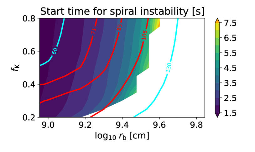
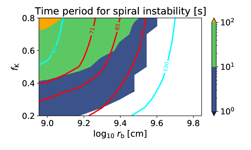
Figure 9: Time after core collapse at which gravitational instabilities in the collapsar disk first set in (top panel) and the duration over which gravitational instabilities are continuously excited during the fallback process (bottom panel), shown in the space of $\{r_{\rm b},f_{\rm K}\}$ for the fiducial progenitor model 250.25. White space indicates models that do not experience gravitational instabilities during fallback accretion. Red contours indicate the inferred primary mass of GW190521 [$M_{\odot}$], together with its 90% confidence limits. Cyan contours delineate final BH masses of 60 $M_{\odot}$ and 130 $M_{\odot}$, which approximately correspond to the lower and upper end of the PI mass gap.

The accretion disks formed in superKN collapsars may become susceptible to gravitational instabilities if their disk mass approaches an order-unity fraction of the BH mass during the fallback evolution process (Sec. 2.2). As shown in Fig. 9, only progenitor cores with high angular momentum (small $r_{\rm b}$ and/or high $f_{\rm K}$) lead to fallback accretion that result in gravitational instabilities. Low-angular momentum cores instead form heavier BHs with relatively smaller disk masses.

The onset time of the instability of typically a few seconds (Fig. 9), representative of all superKN progenitor models investigated here, is determined by the progenitor structure, its rotation profile, and the free-fall timescale. Once triggered, subsequent fallback material collapsing onto the disk continues to excite these instabilities in the collapsar disk for a timescale of seconds to hundreds of seconds (Fig. 9), until viscous draining of the disk becomes fast compared to the free-fall timescale of the remaining outer layers of the progenitor star (roughly $\sim\!10$ s for our fiducial model in Fig. 2).

The onset of the instability manifests itself as the exponential growth of a non-axisymmetric one-arm ($m=1$) density mode in the disk with growth time on the order of the orbital period of the disk, typically followed by exponential growth of an $m=2$ mode (e.g., Kiuchi, K. et al. 2011; Shibata et al. 2021; Wessel et al. 2021). These non-axisymmetric density perturbations give rise to gravitational-wave emission with dominant frequency at the orbital and twice the orbital frequency, respectively (e.g., Wessel et al. 2021).

As long as further fallback keeps the disk in the instability regime defined by Eq. (25), we assume that the dominant gravitational-wave frequencies of these modes are determined by the evolving angular frequency $\Omega_{\rm K,disk}$ of the disk (Eq. 18) with radius $r_{\rm disk}(t)$ (Sec. 2.2). Since $r_{\rm disk}(t)$ monotonically increases with time as the black hole grows and material with larger specific angular momentum enters the disk, the gravitational-wave frequency decreases, sweeping down with a rate and amplitude that depends on the density and angular momentum structure of the progenitor star envelope. The gravitational-wave signal thus exhibits a “sad-trombone” pattern in the time-frequency spectrogram, as opposed to a “chirp” signal generally associated with gravitational waves from compact binary mergers. Examples of the frequency evolution of the disk for different mass models and for high and low specific angular momentum of the progenitor envelope are shown in Fig. 10. Over a large range of the parameter space and progenitor models explored here, superKN collapsars are strong emitters of quasi-monochromatic gravitational waves of duration $\sim\!1-100$ s with a decreasing frequency trend (between $\sim\!0.1-40$ Hz for the $l=m=2$ and $\sim\!\text{few}\times 10^{-2}-25$ Hz for the $l=2$, $m=1$ mode) characteristic of their progenitor stellar structure (see Figs. 9 and 19 for a representative example). If detected, such gravitational-wave signals could reveal information about the rotation profiles of and angular momentum transport in evolved massive stars. The “sad-trombone” feature simultaneously followed by typically two dominant modes separated in frequency space by the instantaneous characteristic disk rotation frequency may prove useful in searching and detecting such sources with gravitational-wave detectors.

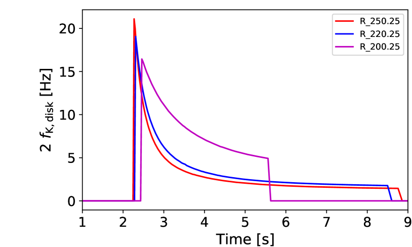
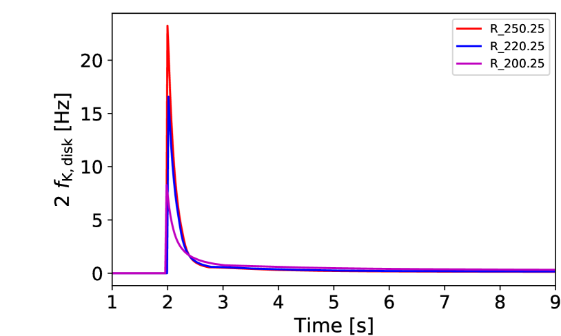
Figure 10: Disk frequency evolution (Eq. 18) for three progenitor models (250.25, 220.25, 200.25) with rotation parameters $p=4.5$, $r_{\rm b}=1.5\times 10^{9}$ cm, and overall small ($f_{\rm K}=0.3$; top) or large ($f_{\rm K}=0.6$; bottom) Keplerian angular momentum parameter. Plotted is twice the orbital angular frequency, which corresponds to the gravitational-wave frequency of the $m=2$ density mode of the gravitationally unstable disk. The frequency evolution is largely controlled by $f_{\rm K}$, with all models reflecting the ‘sad-trombone’ nature of the gravitational-wave signal.

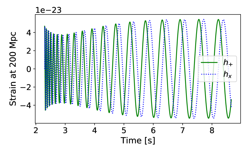
Figure 11: Plus and cross polarization strain amplitudes of the $l=m=2$ mode of gravitational waves resulting from the gravitationally unstable collapsar disk of the fiducial model shown in Fig. 2 with $p=4.5$, $f_{\rm K}=0.3$ and $r_{\rm b}=1.5\times 10^{9}$ cm, assuming a face-on orientation of the accretion disk ($\iota=0$). The emission starts a few seconds after the onset of collapse and persists for several seconds until viscous draining of the disk dominates fallback accretion and the disk becomes stable again at around 9 s after the onset of collapse.

We calculate the gravitational wave strain of emitted gravitational waves as described in Appendix E. Figures 11–14 present results for gravitational-wave emission, evaluated for a typical distance of 200 Mpc, at which superKN events are expected to occur once every $\sim\!3$ years for our fiducial local superKN rate of 10 Gpc^-3 yr^-1 (Sec. 4.1). Figure 11 shows the time evolution of the plus and cross polarization strain calculated for the fiducial progenitor model (Fig. 2) assuming a face-on orientation of the collapsar disk ($\iota=0$). The maximum characteristic strain $h_{c}$ (typically $h_{c}\sim 10^{-24}-10^{-22}$) and the frequency range of the gravitational wave emission vary considerably across the $\{f_{\rm K},r_{\rm b}\}$ parameter space (Figs. 19 and 20, Appendix E).

SuperKN collapsars are multi-band gravitational-wave sources. Figures 12 and 14 compare the gravitational-wave signal in frequency space to the sensitivity of advanced LIGO (aLIGO), Cosmic Explorer (CE), Einstein Telescope (ET), DECi-hertz Interferometer Gravitational wave Observatory (DECIGO), and Big Bang Observer (BBO). Gravitational-wave emission typically starts at a few tens of Hz in the frequency band of aLIGO, CE, and ET, and subsequently drifts into the deciherz regime of DECIGO and BBO as the disk expands. The relative strain amplitude in these two different bands encodes information about the total mass and mass profile of the progenitors (Fig. 12). Lighter progenitors typically give rise to louder gravitational-wave signals over a narrower frequency band for the same rotation profile.

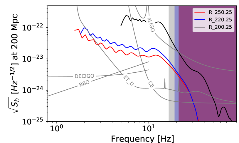
Figure 12: Amplitude spectral density (ASD) of gravitational-wave emission from the collapsar disk, shown for three progenitor models (250.25, 220.25, 200.25) and stellar rotation parameters $p=4.5$, $f_{\rm K}=0.3$, $r_{\rm b}=1.5\times 10^{9}$ cm at an assumed source distance of 200 Mpc. The shaded region for each curve shows the unphysical frequency regime above the maximum disk frequency as plotted in Fig. 10, which is ignored in the SNR calculations. Shown for comparison are the measured or predicted noise curves for aLIGO, CE, ET, DECIGO, and BBO with sensitivity curve data from https://dcc.ligo.org/LIGO-T1500293/public and Yagi & Seto (2011).

The overall magnitude of the amplitude spectral density is largely determined by the progenitor angular momentum as illustrated in Fig. 14. In the limit of high angular momentum (large value of the parameter $f_{\rm K}$) for fixed $r_{\rm b}$, the instability and gravitational-wave emission are triggered earlier than for smaller values of $f_{\rm K}$ (cf. Fig. 9). This is because matter deposition in the disk at early times is enhanced (rather than direct fallback onto the black hole). Under these conditions, the gravitational-wave signal is relatively weak due to the small disk and BH mass. Owing to enhanced viscosity and enhanced accretion during the instability epoch, disks that become unstable early on tend to stay relatively light; the gravitational-wave signal thus remains relatively weak throughout the fallback process. As a result, these signals tend to peak late and thus in the decihertz regime, which may only render them detectable there for Mpc distances. A non-detection in the high-frequency band may thus be indicative of the angular momentum budget of the progenitor star. In the other limit of low angular momentum (small value of the parameter $f_{\rm K}$ and large $r_{\rm b}$), the accretion disk may never become susceptible to the instability and gravitational-wave emission may be negligible (cf. Fig. 9). Hence, there exists an intermediate regime of progenitor angular momentum (intermediate values of $f_{\rm K}$) in which the gravitational wave strain becomes maximal. For the given parameters of our fiducial progenitor model, this optimum is reached for $f_{\rm K}\approx 0.2$, which is also reflected by the detection horizons (Figs. 13, 21).

We calculate a detection horizon for these events assuming an optimal matched filter and an SNR of 8 (see Appendix E for details). We find a detection horizon of $\sim$5 Mpc (aLIGO), $\sim$300 Mpc (ET), $\sim$250 Mpc (CE), and $\sim$425 Mpc (DECIGO) for our fiducial model with mass $250.25M_{\odot}$, $f_{\rm K}=0.3$, and $r_{\rm b}=1.5\times 10^{9}$ cm. A parameter space study of the detection horizons is presented in Fig. 13, showing that third-generation detectors (ET, CE) as well as DECIGO are able to detect gravitational waves from superKN collapsars at distances of typically a few hundred Mpc up to a few Gpc. Detection horizons for aLIGO are typically limited to $\lesssim 100$ Mpc (Fig. 21, Appendix E). BBO will be particularly sensitive to the lowest-frequency sources with low angular momentum in the progenitor ‘core’ (medium to large values of $r_{\rm b}$) and typically reach several hundred Mpc to several Gpc. (Fig. 21, Appendix E).

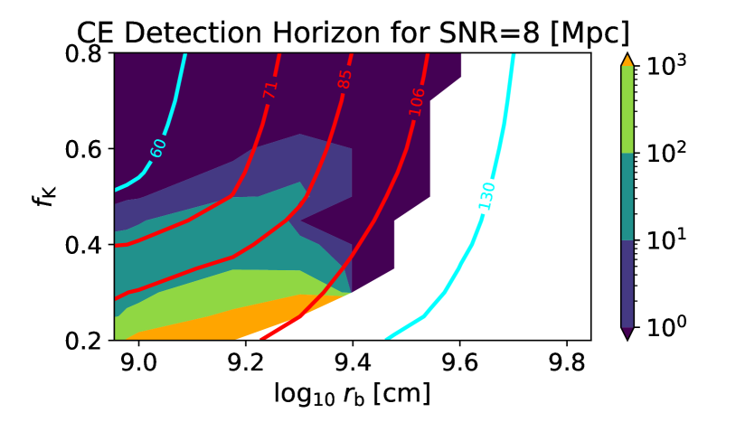
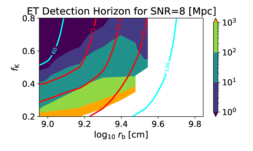
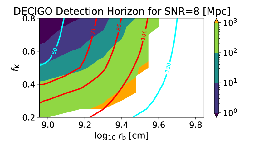
Figure 13: Detection horizons of gravitational waves from our fiducial model shown in Fig. 2 with $p=4.5$, $f_{\rm K}=0.3$ and $r_{\rm b}=1.5\times 10^{9}$ cm for Cosmic Explorer (top), the Einstein Telescope (center), and DECIGO (bottom), assuming optimal matched filtering and a signal-to-noise ratio of 8. For progenitors with medium to low rotation, these detectors may be able to detect gravitational waves from superKN collapsars at distances of typically a few hundred Mpc up to a few Gpc. These estimates are based on the corresponding physical frequency regime as indicated in Fig. 10. The sharp decrease in detection horizon for CE at $\log r_{\rm b}\gtrsim 9.4$ is due to low-frequency emission below 10 Hz (below CE’s sensitivity band). Contours delineate final BH masses as in previous figures.

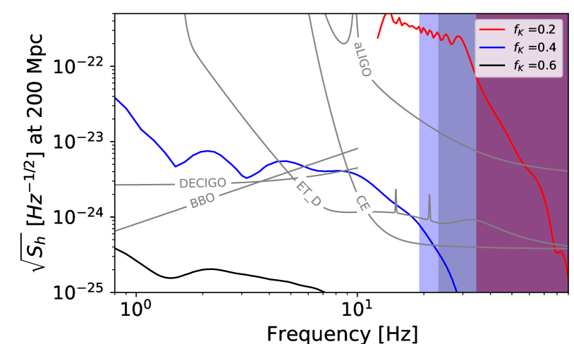
Figure 14: Same as Fig. 12 but for the progenitor model 250.25 with $p=4.5$, $r_{\rm b}=1.5\times 10^{9}$ cm and different values of the Keplerian fraction, $f_{\rm K}=0.2,0.4$ and $0.6$. Relatively low to medium angular momentum models (here $f_{\rm K}\approx 0.2$) generate a stronger signal in all detectors (with detection horizon $\sim$ 400 Mpc with aLIGO at an SNR of 8) compared to cases with higher angular momentum (large values of $f_{\rm K}$). The $f_{\rm K}=0.6$ model would only be detectable by BBO with a distance up to 100 Mpc at an SNR of 8 (cf. Fig. 21).

5.3 GW190521

Our work has several potential implications for the gravitational wave event GW190521 (Abbott et al., 2020). Firstly, as already discussed, in the standard interpretation of GW190521 as a binary BH coalescence, mass loss associated with the birth of one or both of the constituent BHs can place them in the nominal PI mass gap “from above”, even if they would have been above the PI gap if all of the star’s mass were accreted at the time of core collapse (Fig. 4, top panel). To generate a BH with a mass consistent with the more massive member of GW190521 of $\sim 88M_{\odot}$ (Abbott et al., 2020) from a star with a helium core nominally above the gap, would require the ejection of $\gtrsim 50M_{\odot}$ of ejecta (most of it $r$-process enriched; Sec. 2.2). In a direct sense, superKNe probe one channel for forming BHs in the PI mass gap.

Our scenario requires a fast rotating pre-collapse star and predicts that the magnitude of the BH spin would be nearly maximal ($a_{\rm BH,fin}\sim 1$; Fig. 18, bottom panel). Although a low orbit-aligned spin $\chi_{\rm eff}\lesssim 0.35$ (90% confidence) was measured for GW190521, there is some evidence for a large spin component in the binary plane (Abbott et al., 2020). However, assuming that the progenitor stars can retain large rotation rates (see however Spruit, 2002; Fuller & Ma, 2019) and the progenitor of GW190521 formed from an isolated stellar binary through common envelope evolution (e.g., Belczynski et al., 2016), stable mass transfer (e.g., van den Heuvel et al., 2017; van Son et al., 2021), or via chemically homogeneous evolution driven by tidal interactions (e.g., Maeder & Meynet, 2000; de Mink & Mandel, 2016; Marchant et al., 2016), one would expect the stellar angular momentum vector—and hence that of the BHs formed from the collapse—to be aligned with the orbital angular momentum (Mandel & de Mink, 2016).

In the case of rapidly rotating progenitors, we speculate that misaligned spins could arise from a kick imparted to the BH by mass loss in the disk winds. Our calculations in Sec. 5.2 indicate that the formed disks can become self-gravitating and hence will be subject to bar-mode like instabilities, generating non-axisymmetric spiral density waves. The latter could impart a non-axisymmetric component to the wind mass loss, which would endow the BH with an effective kick. To significantly misalign the spins without breaking the binary, the natal kick must be comparable to the pre-collapse orbital velocity of the system, $v_{\rm kick}\sim 300$ km s^-1 (e.g., Kalogera 1996; Callister et al. 2021). Given the characteristic wind ejecta speed $v_{\rm ej}\sim 0.1$ c, from momentum conservation an asymmetry in the disk mass-loss rate or velocity at the level of $\gtrsim v_{\rm kick}/v_{\rm ej}\sim 10^{-2}$ would be sufficient to impart significant spin-orbital misalignment. Although self-gravitating instabilities result in non-axisymmetric disk density fluctuations at the level $\delta\rho/\rho\gtrsim 0.1$, quantifying the extent to which these impart non-axisymmetric mass-loss will require additional GRMHD simulations of the disk outflows in the regime of massive, self-gravitating disks.

In an alternative approach, Shibata et al. (2021) interpret GW190521 as gravitational waves from a non-axisymmetric instability similar to those discussed in Sec. 5.2 in a massive BH–disk system, thought to originate from the collapse of a massive star. In contrast to the BH–torus systems of fixed mass numerically evolved by Shibata et al. (2021), in an astrophysical setting mass is continuously fed to the disk at a rate $\dot{m}_{\rm fb,disk}$ due to fallback of the progenitor envelope (Sec. 2.2). If the accretion disk approaches the gravitationally unstable regime its mass evolution $M_{\rm disk}(t)$ is dominated by the addition of fallback material through $\dot{m}_{\rm fb,disk}$. The associated timescale over which the fallback rate changes is $\tau_{\dot{m}_{\rm fb,disk}}\propto t^{\alpha}$, where $\alpha\approx 1$ (Siegel et al. 2019 and Sec. 2.2). This is reflected by the fact that disks for the progenitor models considered here become gravitationally unstable on a timescale of a few seconds after BH formation, and this instability phase then lasts for a few seconds to tens of seconds (Fig. 9, Sec. 5.2). Generating a gravitational-wave signal of only a few cycles and duration $t_{\rm GW}\sim 0.1$ s as required by GW190521 (Abbott et al., 2020) with comparatively negligible amplitude thereafter thus requires a fallback rate given by the total mass of the BH–disk system divided by the duration of the signal of $\dot{m}_{\rm fb,disk}>(M_{\bullet}+M_{\rm disk})/t_{\rm GW}\sim 650-1000\,M_{\odot}\,\text{s}^{-1}$ for the configurations considered by Shibata et al. (2021). While fallback rates of the order of up to $\sim\!30-40\,M_{\odot}\,\text{s}^{-1}$ may be reached realistically (cf., e.g., Fig. 2), fallback rates that are larger by one or two orders of magnitude seem implausible even with the most compact progenitor models possible (Sec. 2.1). These fallback rates also set limits on the compactness and thus on the gravitational-wave frequency of possible BH–disk systems—the frequency of gravitational-wave emission may be in tension with GW190521 as well. While a frequency around $\sim\!60$ Hz of GW190521 may not be impossible per se, our unstable BH–disk systems are typically not compact enough to reach such high frequencies even for an $l=m=2$ mode and instead strongly prefer maximum frequencies below 20-30 Hz (Fig. 10). Another consequence of the weaker gravitational wave signals that we predict from massive collapsars are much closer detection horizons, which for Advanced LIGO at O3 sensitivity amount to $\lesssim 100$ Mpc (Fig. 21, Appendix E); it is unlikely that a superKN transient from GW190521 would have gone undetected by existing wide-field optical surveys at such close distances.

5.4 Implications for Galactic $r$-Process Enrichment

Although the massive collapsars studied here are probably less common by a factor $\gtrsim 10-30$ than the bulk of ordinary collapsars (Sec. 4.1), they can in principle generate $\sim 10$ times more $r$-process ejecta mass for similar progenitor angular momentum structure. The contribution of superKNe to total $r$-process production in the Universe could therefore be non-negligible relative to that of ordinary collapsars.

SuperKNe are probably too rare to explain the occurrence of individual $r$-process pollution events in small dwarf galaxies (e.g., Ji et al. 2016), but this does not exclude them from contributing to larger stellar systems. The total mass of $r$-process elements in the Milky Way is only $\sim 10^{4}M_{\odot}$, so given an $r$-process yield of $\gtrsim 10M_{\odot}$ per superKNe, the number of contributing events must be $\lesssim 1000$ and probably $\lesssim 100$ (accounting for the dominant contribution likely coming from other channels such as lower mass collapsars and neutron star mergers).

Depending on the efficiency of gas mixing and retention in the environments of superKNe, subsequent generations of star formation could produce a modest number of extremely $r$-process-enriched stars. The dilution mass of the interstellar medium into which the superKN ejecta is mixed, can be estimated as (e.g., Macias & Ramirez-Ruiz 2019)

$$M_{\rm dil}\approx 2\times 10^{7}M_{\odot}\left(\frac{E_{\rm kin}}{5\times 10^{53}\rm erg}\right)^{0.97}\left(\frac{n}{\rm cm^{-3}}\right)^{-0.062},$$ (36)

where we have assumed $10$ km s^-1 for the sound speed of the interstellar medium. The value of $M_{\rm dil}$ in superKNe is larger than in ordinary SNe ($E_{\rm kin}\sim 10^{51}$ erg) or ordinary collapsars ($E_{\rm kin}\sim 10^{52}$ erg) by a factor of $\gtrsim 10-100$.

The total amount of $r$-process material generated by superKNe is larger than ordinary collapsars by a similar factor $\sim 10$, while the production $\sim 0.1-0.5M_{\odot}$ of ⁵⁶Ni and hence ⁵⁶Fe (Fig. 5) are similar to ordinary collapsars. If a superKN were to occur in otherwise pristine material at very low metallicity (perhaps an questionable idealization given that SNe tend to be spatially and temporally clustered), the next generation of stars which form from this material could possess a metallicity as low as [Fe/H] $\sim-5$ and a Europium abundance as high as [Eu/Fe] $\sim 5$, much higher than the current record holder (Reichert et al. 2021). This abundance combination would also contrast strongly with the chemical signatures of PI SNe (e.g., Woosley et al. 2002; Aoki et al. 2014), for which a large quantity of iron group elements but no $r$-process elements are produced.

6 Conclusions

We have explored the collapse of rotating very massive $\gtrsim 130M_{\odot}$ helium stars and predicted their nucleosynthetic, electromagnetic, and gravitational waves signatures. Our conclusions can be summarized as follows.

• Building on Siegel, Barnes, & Metzger (2019), we present a semi-analytic model for the BH accretion disk in collapsars and its associated outflows which predict the quantity and composition of the disk wind ejecta, as well as the final BH mass and spin, given an assumed angular momentum structure of the progenitor star. The accretion regimes are calibrated based on the results of numerical GRMHD simulations and analytic scaling relations (Appendix A). Although the radial angular momentum structure of the progenitor star at collapse is uncertain theoretically, our approach allows us to cover a wide portion of the physically allowed parameter space. Applied to “ordinary” low-mass collapsars, the model predicts accretion luminosities and durations broadly consistent with long GRB observations.

• Our main application is to massive collapsars, originating from progenitor stars with final helium core masses $\sim 125-150M_{\odot}$, which avoid pair instability SNe and nominally (in the case of zero mass ejection) would create BHs above the PI mass-gap. Analogous to lower-mass collapsars, as the fall-back accretion rate declines in time, the composition of the disk outflows systematically evolve from heavier to lighter elements (Fig. 3). Across a wide parameter space of progenitor rotational properties, we find total wind ejecta masses $\sim 10-50M_{\odot}$, of which $\sim 10-60\%$ is composed of $r$-process nuclei, including a sizable quantity of lanthanide elements associated with heavy $r$-process production. The remaining ejecta is primarily unprocessed material (assumed to be ⁴He in our models) and a modest quantity $\sim 0.1-1M_{\odot}$ of ⁵⁶Ni, formed from the brief hot, proton-rich phases of the disk evolution.

• The radioactive decay of $r$-process nuclei and ⁵⁶Ni in the ejecta of massive collapsars powers a months-long transient with a peak luminosity $\sim 10^{42}$ erg s^-1 (Fig. 7), which we refer to as a “superKN”. The spectral energy distribution of superKNe near maximum light peaks at several microns due to the large opacity of the lanthanide elements (Fig. 8), similar to lanthanide-rich kilonovae from neutron star mergers. Although the bolometric light curves of superKNe are broadly similar to common types of core-collapse SNe, their combination of extremely red colors and high-velocity spectral features ($v_{\rm ej}\sim 0.1$ c) should render superKNe distinguishable from other transient classes.

  Our radiative transfer calculations have assumed a homogeneous ejecta structure; if the ejecta instead exhibits significant radial stratification, particularly a low lanthanide abundance in the highest velocity outermost layers, then the early light curve could be substantially brighter and bluer than our baseline predictions.

• Even for a progenitor stars well above the PI mass gap at collapse, the final BH remnant can populate the entire mass gap between $\sim 55-130M_{\odot}$ due to disk wind mass-loss (e.g., Fig. 4; Tab. 1). SuperKNe therefore probe one mechanism for populating the PI mass gap “from above”. The BHs formed through this channel are predicted to be rapidly spinning due to the large accretion of angular momentum, with final Kerr parameter $a_{\rm BH,fin}\sim 1$. If the BH is formed in a binary, we speculate that its spin angular momentum axis could become misaligned with that of the binary angular momentum due to non-asymmetric mass-outflows associated with the gravitationally-unstable phases of the accretion (Sec. 5.2). Future numerical simulation work is necessary to explore this possibility quantitatively.

• One avenue to discover SuperKNe is via wide-field optical/infrared surveys. A 5-year survey with the Roman Space Telescope similar to that planned for Type Ia SNe, could potentially detect $\sim 1-20$ superKNe out to redshift $z\simeq 1$, for an assumed $z=0$ superKN rate of $\sim 10$ Gpc^-3 yr^-1. SuperKNe could also be discovered by LSST, but the detection rate is lower because the predicted emission peaks at redder wavelengths than covered by the LSST bands. Measurements or limits on the occurrence rate of superKNe would constrain the birth rate of PI mass gap BHs via this channel (for comparison, the local rate of GW190521-like mergers is $\sim 1$ Gpc^-3 yr^-1; Abbott et al. 2020). SuperKNe may also be detectable following (particularly energetic) GRBs with JWST after the GRB afterglow has faded.

• The large kinetic energies of the superKN ejecta $\gtrsim 10^{53}$ erg results in a bright, long-lived synchrotron radio transient as the ejecta decelerates via shock interaction with the circumstellar medium (Sec. 5.1). However, the slow evolution of the radio emission for typical circumstellar densities will render these radio sources challenging to identify as radio transients (they may appear as luminous persistent sources in star-forming dwarf galaxies, for example; Eftekhari et al. 2020).

  If superKNe occur inside gaseous AGN disks, shock interaction with the dense disk material could substantially enhance the optical luminosity of the event relative to that powered by radioactivity alone. This offers a speculative explanation for the claimed optical counterpart of GW190521 (Graham et al., 2020), provided it represents a gravitational wave burst from a core collapse event (Shibata et al., 2021) instead of a black hole merger (however, see Sec. 5.3).

• The massive accretion disks from massive collapsars can become gravitationally unstable, generating gravitational wave emission as a result of non-axisymmetric density fluctuations. The predicted duration of the gravitational waves is several seconds or longer (calling into question the core-collapse origin for GW190521 proposed by Shibata et al. 2021, Sec. 5.3), while the frequency range overlaps the sensitivity window of ground-based (e.g., LIGO/CE/ET) and space-based intermediate-frequency gravitational-wave detectors (e.g., DECIGO, BBO). Unlike the gravitational wave signal of compact binary mergers, which increase in frequency and amplitude with time (“chirp”), the gravitational wave signals of collapsar disks decreases in frequency as the disk radius grows (“sad-trombone”). Our simple estimates suggest that gravitational waves from massive collapsar disks are detectable by CE/ET/DECIGO to distances of up to several hundred Mpc (Figs. 12, 13, 14), interior to which the event rate could be as high as once every few years.

• SuperKNe are unlikely to contribute dominantly to the total production of $r$-process elements in the Universe, compared to neutron star mergers or ordinary low-mass collapsars, because the progenitors are disfavored by the initial mass function of stars. However, their extremely $r$-process-rich but iron-poor ejecta could in principle seed the creation of a small fraction of stars with abundance ratios more extreme than currently known metal-poor $r$-process-enhanced stars (e.g., [Eu/Fe] $\sim 5$).

Appendix A Dependence of Critical Accretion Rates on BH Mass

Here we estimate various critical accretion rates which enter our calculations in Sec. 2.2. We focus on deriving the scaling laws as a function of the effective $\alpha$ viscosity parameter and the BH mass $M_{\bullet}$, normalizing our final results to those obtained by one-dimensional (e.g., Chen & Beloborodov 2007) and three-dimensional MHD simulations (e.g., De & Siegel 2020).

A.1 Ignition Accretion Rate

We begin with the critical accretion rate $\dot{M}_{\rm ign}$, below which neutrinos can no longer efficiently cool the inner regions of the disk and lead to its self-neutronization.

At the transition between efficient neutrino cooling and adiabatic evolution, the midplane temperature $T$ is determined by balancing the specific rate of neutrino cooling $\dot{q}_{\nu}\propto T^{6}$ in the optically-thin limit (due to the capture of relativistic electrons and positrons on free nuclei; e.g., Qian & Woosley 1996; Di Matteo et al. 2002), with the rate of viscous heating,

$$\dot{q}_{\rm visc}\approx\frac{9}{4}m_{\rm p}\nu\Omega^{2}\approx\frac{9}{4}\alpha m_{\rm p}r^{2}\Omega^{3}\left(\frac{H}{r}\right)^{2},$$ (A1)

where $\nu=\alpha c_{\rm s}H\simeq\alpha R^{2}\Omega(H/r)^{2}$ is the kinematic viscosity and $m_{p}$ is the proton mass. We have assumed a Keplerian disk with angular velocity $\Omega\simeq\Omega_{\rm K}=(GM_{\bullet}/r^{3})^{1/2}$, midplane sound speed $c_{\rm s}=H\Omega$ and aspect ratio $H/r$. Since $H/r\sim\mathcal{O}(1)$ once advective cooling competes with radiative cooling (e.g., Di Matteo et al. 2002), we have $H/r\sim\mathrm{constant}$ at the transition to an advective disk from an efficiently neutrino-cooled disk. This gives,

$$T^{6}\propto\alpha r^{2}\Omega^{3}.$$ (A2)

We also assume that, near the transition point to an advective disk, radiation pressure dominates over gas pressure in the disk midplane, i.e. the midplane pressure obeys $P\propto T^{4}$. From vertical hydrostatic equilibrium, we then have

const. $$\sim \left(\frac{H}{r}\right)^{2}\approx\frac{c_{\rm s}^{2}}{r^{2}\Omega^{2}}\approx\frac{P/\rho}{r^{2}\Omega^{2}}\propto\frac{\alpha T^{4}r}{\Omega\dot{M}}$$ (A3)

$$\Rightarrow T^{4}\propto\frac{\dot{M}\Omega}{\alpha r}$$

where $\rho$ is the midplane density and in the final line we have used the fact that the local disk mass $M_{\rm d}\propto\rho r^{2}H$ accretes on the local viscous time $t_{\rm visc}\propto\nu/r\sim\alpha^{-1}\Omega^{2}(H/r)^{-2}$, i.e.

$$\dot{M} \propto \frac{M_{\rm d}}{t_{\rm visc}}\propto\frac{\rho r^{2}H}{\alpha^{-1}\Omega^{-1}(H/r)^{-2}}\propto\alpha\rho\Omega r^{3}\left(\frac{H}{r}\right)^{3}$$ (A4)

$$\Rightarrow \rho\propto\frac{\dot{M}}{\alpha\Omega r^{3}}.$$

Combining Eqs. (A2), (A3), we obtain

$$\dot{M}\propto\alpha^{5/3}r^{7/3}\Omega.$$ (A5)

Scaling $r$ to the radius of the innermost stable circular orbit, $r_{\rm ISCO}\propto M_{\bullet}$, we have $r\propto M_{\bullet}$ and $\Omega\propto M_{\bullet}^{-1}$, thus giving

$$\dot{M}_{\rm ign}\propto\alpha^{5/3}M_{\bullet}^{4/3}.$$ (A6)

A derivation of this scaling in the general-relativistic context is given in De & Siegel (2020). The scaling $\dot{M}_{\rm ign}\propto\alpha^{5/3}$ has been verified in 1D models (Chen & Beloborodov, 2007) for BH masses $M_{\bullet}\approx 3M_{\odot}$. However, the scaling should hold for the higher values of $M_{\bullet}$ of interest in this paper because the assumptions which enter the above derivation (i.e., optically thin cooling, radiation pressure dominating over gas pressure at the advective transition) only strengthen with increasing BH mass. In particular, the ratio of radiation to gas pressure,

$$\left.\frac{T^{3}}{\rho}\right|_{\dot{M}_{\rm ign}}\propto r^{5/3}\Omega^{3/2}\propto M_{\bullet}^{1/6},$$ (A7)

increases with $M_{\bullet}$. Other forms of neutrino cooling, particularly arising from the annihilation of electron-positron pairs into neutrino-antineutrino pairs, will dominate over the pair-capture rates entering the radiative cooling rate at sufficiently high $T^{3}/\rho$ (e.g., Qian & Woosley 1996), changing the above scalings. However, the weak $M_{\bullet}$-dependence in Eq. (A7) suggests that this is not likely to occur for even the highest BH masses $M_{\bullet}\sim 100M_{\odot}$ of interest in this paper.

A.2 Neutrino Opaque and Trapping Thresholds

We now consider the accretion rate $\dot{M}_{\nu,\rm r-p}$, above which the inner disk is optically thick to neutrinos. The vertical optical depth through the disk obeys

$$\tau_{\nu}\propto\Sigma\kappa\propto\rho HT^{2},$$ (A8)

where $\sigma\propto T^{2}$ is the energy-dependent absorption cross section with which electron neutrinos or antineutrinos are absorbed by free neutrons or protons, respectively. Using Eqs. (A3) and (A4) for $T$ and $\rho$, and again taking $H/r\sim\text{const.}$, we find:

$$\tau_{\nu}\propto\frac{\dot{M}^{3/2}}{\alpha^{3/2}\Omega^{1/2}r^{5/2}}.$$ (A9)

Evaluating the marginally thick condition $\tau_{\nu}=1$ at $r\approx r_{\rm ISCO}$, we obtain

$$\dot{M}_{\nu,\rm r-p}\propto\alpha M_{\bullet}^{4/3}.$$ (A10)

A.3 Neutrino Trapping Threshold

Finally, consider the “trapping” accretion rate $\dot{M}_{\rm tr}$, above which the thermal energy released by the accretion flow is advected into the BH faster than it can be radiated through neutrinos. Equating the neutrino diffusion timescale out of the disk midplane $t_{\rm diff}\sim\tau_{\nu}(H/c)$ with the inwards flow time $\sim r/v$, we find that neutrinos are trapped for $\tau_{\nu}>(c/v)(r/H)$. Using $v\sim\nu/r$ for the inflow velocity of a steady disk and Eq. (A8), and again taking $H/r\sim\text{const.}$, the trapping condition can be written

$$\Sigma\nu T^{2}>r.$$ (A11)

Finally, recalling that $\nu\Sigma\propto\dot{M}$ for steady accretion, then using Eq. (A3) and evaluating Eq. (A11) at $r=r_{\rm ISCO}$, we find

$$\dot{M}_{\rm tr}\propto\alpha^{1/3}M_{\bullet}^{4/3}.$$ (A12)

Appendix B Production of ⁵⁶Ni in disk winds and dissociation threshold

Assuming the dominant seed particle formation process in the disk wind outflow is ⁴He(2$\alpha,\gamma$)¹²C, rather than the neutron-catalyzed reaction ⁴He($\alpha n,\gamma)^{9}$Be($\alpha,n)^{12}$C in neutron-rich environments $Y_{e}\ll 0.5$ (Woosley & Hoffman, 1992), the destruction of $\alpha$-particles in disk winds proceeds as (Roberts et al., 2010)

$$\frac{dY_{\alpha}}{d\tau}\approx-14\rho^{2}Y_{\alpha}^{3}\lambda_{3\alpha},$$ (B1)

where $Y_{\alpha}$ is the abundance of $\alpha$-particles, $\lambda_{3\alpha}(T)$ is the temperature-dependent triple-alpha rate coefficient, and the factor of 14 is due to assuming $\alpha$-captures cease at ⁵⁶Ni. Furthermore, $d\tau=-(\tau_{\rm d}/3T)dT$, where $\tau_{\rm d}$ is the expansion time of the outflow around the point of $\alpha$-particle formation. We take $\tau_{\rm d}\approx 5-30\,\text{ms}$ typical of expansion time scales of such accretion disk winds (Siegel & Metzger, 2018; Siegel et al., 2019). Integration of Eq. (B1) yields the resulting abundance of seed particles (Roberts et al., 2010)

$$Y_{\rm seed}=\frac{1}{56}\left\{1-[1+35(\tau_{\rm d}/{\rm ms})s_{\rm f}^{-2}]^{-1/2}\right\}.$$ (B2)

Here, $s_{\rm f}$ is the final entropy in $k_{\rm B}$ per baryon, which we estimate by $s_{\rm f}\approx s_{\rm m}=s_{\rm m,rad}+s_{\rm m,N}$, where

$$s_{\rm m,rad} = \frac{11\pi^{2}k^{3}m_{\text{p}}}{45c^{3}\hbar^{3}}\frac{T_{\rm m}^{3}}{\rho_{\rm m}}$$ (B4)

$$\approx 21\left(\frac{r_{\rm disk}}{5r_{\rm g}}\right)^{-\frac{3}{8}}\left(\frac{\dot{M}}{10^{-4}M_{\odot}\,s^{-1}}\right)^{-\frac{1}{4}}\mskip-5.0mu\left(\frac{\alpha}{0.01}\right)^{\frac{1}{4}}$$

$$\times\left(\frac{M_{\bullet}}{3M_{\odot}}\right)^{\frac{7}{8}}\left(3h_{z,\text{disk}}\right)^{\frac{9}{4}},$$

is the entropy of radiation in the disk midplane and

$$s_{\rm m,N}\approx 13.3+{\rm ln}\left(\frac{(T_{\rm m}/1\text{MeV})^{3/2}}{\rho_{\rm m}/10^{7}\text{g}\,\text{cm}^{-3}}\right)$$ (B5)

is the entropy in the non-relativistic nucleons. The disk midplane density $\rho_{\rm m}$ and temperature $T_{\rm m}$ are calculated using an $\alpha$-disk model as in Appendix A (see also Siegel et al. 2019). We translate Eq. (B2) into a mass fraction $X_{{}^{56}\mathrm{Ni}}$ and $X_{\mathrm{He}}\approx 1-X_{\rm seed}$ by assuming that seed particles are mostly within the iron peak (charge numbers $24\leq Z\leq 28$), using the nucleosynthesis results of Siegel et al. (2019).

At late times during the fallback process (low accretion rates), the accretion disk must be hot and dense enough to dissociate $\alpha$-particles as well as heavier nuclei of the infalling stellar material into individual nucleons, a requisite for the synthesis of ⁵⁶Ni in disk outflows. We estimate the time of this transition to a state in which dissociation into individual nucleons becomes suppressed by considering a fluid of neutrons, protons, and $\alpha$-particles with a proton fraction $Y_{e}=0.5$ and determining the state in which half of the $\alpha$-particles are dissociated. Assuming that nuclear statistical equilibrium holds (a good assumption as our disk midplane temperatures typically stay above 0.5 MeV), this can be estimated from the Saha equation (Shapiro & Teukolsky, 1983)

$$X_{\rm nuc}^{4}=1.57\times 10^{4}X_{\alpha}\rho_{{\rm m},10}^{-3}T_{{\rm m},10}^{9/2}\exp\left(-\frac{32.81}{T_{{\rm m},10}}\right),$$ (B6)

where $X_{\rm nuc}=2X_{\rm p}=2X_{\rm n}$ is the mass fraction of nucleons, and $\rho_{{\rm m},10}$ and $T_{{\rm m},10}$ denote the midplane density and temperature in $10^{10}\,\text{g}\,\text{cm}^{-3}$ and $10^{10}$ K, respectively. Expressing $X_{\rm nuc}=1-X_{\alpha}$ and setting $X_{\alpha}=0.5$, Eq. (B6) can be solved numerically for the transition time $t_{\rm diss}$ upon inserting $\rho_{\rm m}$ and $T_{\rm m}$ as obtained from the numerical evolution of Eqs. (9)–(14). The time-dependence of the functions $\rho_{\rm m}$ and $T_{\rm m}$ is determined by the evolution of $M_{\bullet}$, $M_{\rm disk}$, and $r_{\rm disk}$. At $t>t_{\rm diss}$ we set $Y_{\rm seed}=0$ in Eq. (B2), discarding any potential ⁵⁶Ni production after this time.

Appendix C Resolution studies

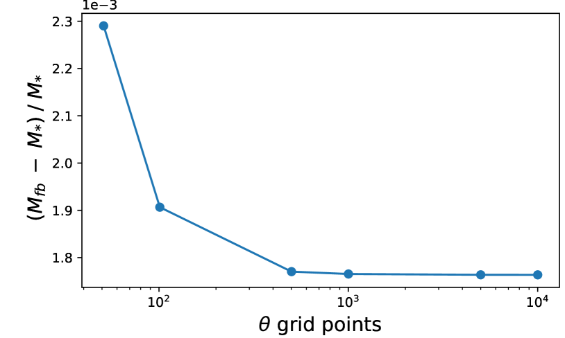
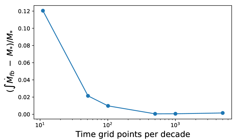
Figure 15: Convergence test for model 250.25. Top: relative error in computing the total mass of the star $M_{\star}$ using a grid discretized in both polar angle and radius, showing that at the fiducial angular resolution of $n_{\theta}=1001$ the relative error $\lesssim 0.0018$ is dominated by the radial resolution of the progenitor model. Bottom: total stellar mass as computed by numerical integration of Eqs. (9)–(14) with fixed angular resolution $(n_{\theta}=1001)$, varying the time step. For sufficiently high temporal resolution, the relative error of $\lesssim 0.002$ is again dominated by the radial discretization of the progenitor model, consistent with the error budget shown in the top panel.

We have performed numerical convergence tests to check convergence of nucleosynthesis results from our collapsar model (Sec. 2.3) and to determine optimal resolution for our numerical collapsar evolution calculations (Sec. 2.2). Figure 15 shows results of two convergence tests to determine optimal discretization for the polar coordinate and for time integration. The top panel illustrates that at our fiducial resolution in the polar angle of $n_{\theta}=1001$ the relative error in computing the total mass of the star by numerical integration is dominated by the radial resolution of the progenitor model (relative error of $\lesssim 0.0018$). The bottom panel indicates that for sufficiently high angular resolution ($n_{\theta}\sim 1001$) and sufficiently large number of time steps of several hundred to $10^{3}$, the relative error in computing the stellar mass by numerical integration of Eqs. (9)–(14) is again dominated by the radial discretization of the progenitor model. The relative error of $\lesssim 0.002$ in this case is consistent with the error budget obtained for the corresponding convergence test in the polar angle. This shows that our results are converged with roughly $10^{3}$ grid points both in $\theta$ an in time, which we employ for all model runs.

Appendix D Results for ordinary collapsars and GRB properties

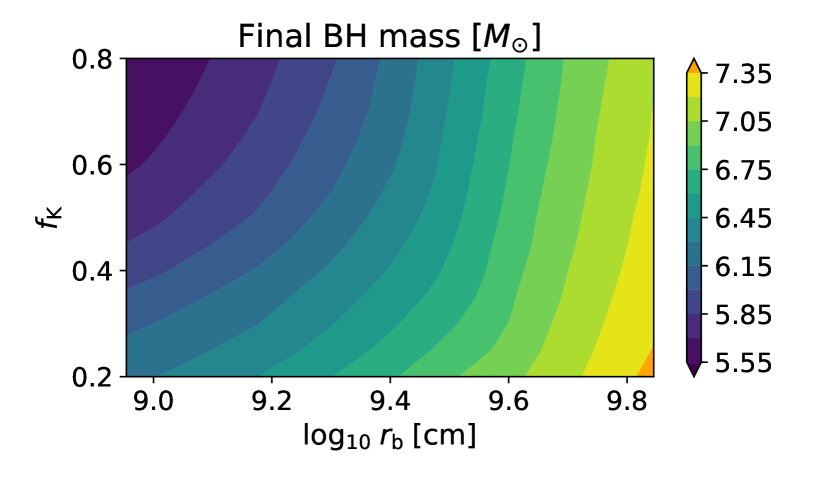
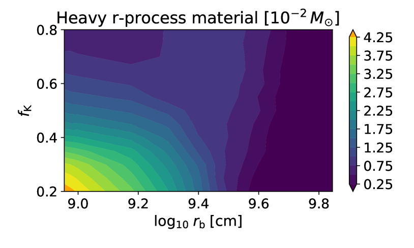
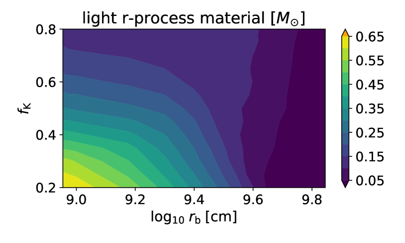
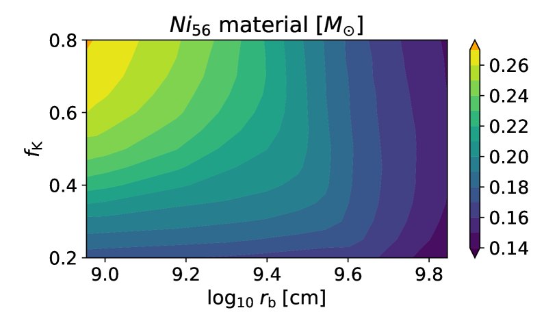
Figure 16: Scan of the parameter space for model E20 of Heger et al. (2000). Shown are the final BH mass (top), the total ejected mass [$M_{\odot}$] in heavy ($A>136$) $r$-process elements (center top), in light ($A<136$) $r$-process elements (center bottom), and ⁵⁶Ni (bottom).

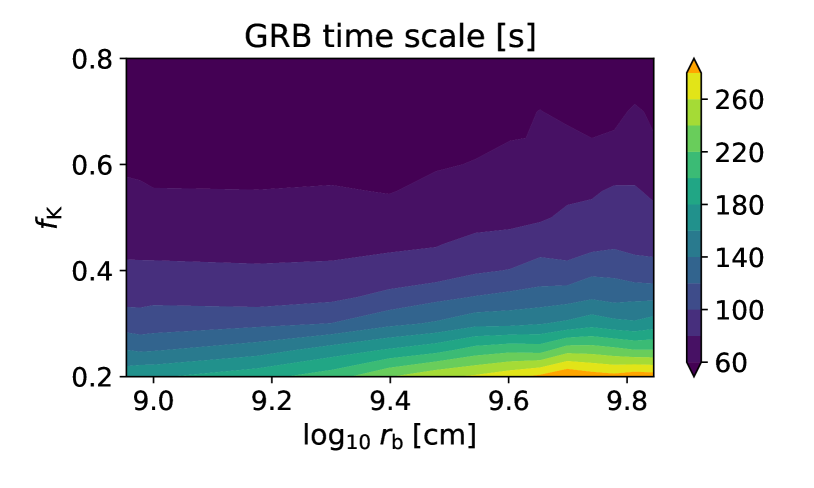
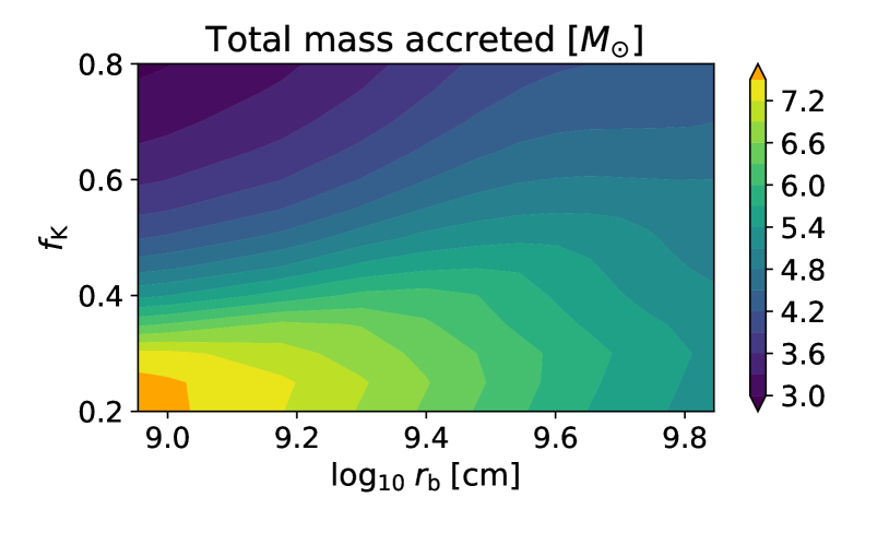
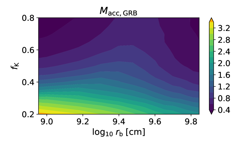
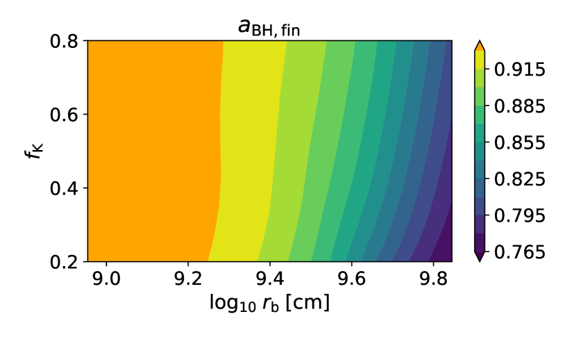
Figure 17: Scan of the parameter space for model E20 of Heger et al. (2000). Shown are the GRB timescale $t_{\rm GRB}$ (top), total accreted mass [$M_{\odot}$] (top center), and accreted mass $M_{\rm GRB}$ during the GRB phase [$M_{\odot}$] (bottom center), and final dimensionless BH spin $a_{\rm BH,fin}$ (bottom).

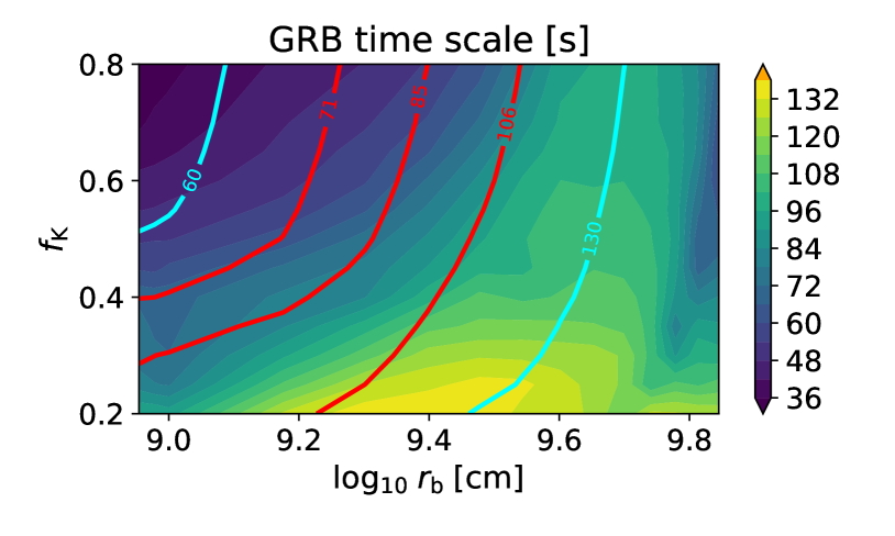
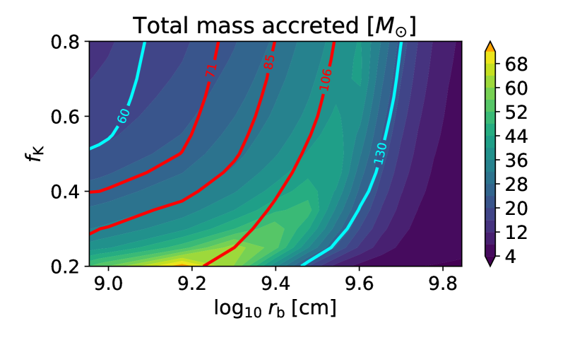
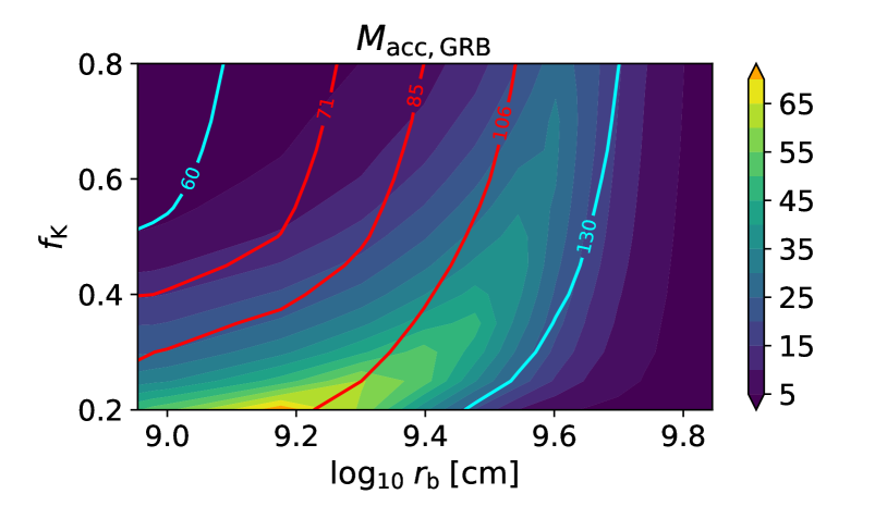
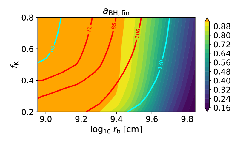
Figure 18: Scan of the parameter space for model 250.25. Shown are the GRB timescale $t_{\rm GRB}$ (top), total accreted mass [$M_{\odot}$] (center top), accreted mass $M_{\rm GRB}$ during the GRB phase [$M_{\odot}$] (center bottom), and final dimensionless BH spin $a_{\rm BH,fin}$ (bottom). Red contours indicate the inferred primary mass of GW190521 [$M_{\odot}$], together with its 90% confidence limits. Cyan contours delineate final BH masses of 60 $M_{\odot}$ and 130 $M_{\odot}$, which approximately correspond to the lower and upper end of the PI mass gap.

Figure 16 presents results for model E20 of Heger et al. (2000), one representative case for ordinary collapsars below the PI BH mass gap. We vary the parameters of the adopted progenitor rotation profile (cf. Eq. (2)) within ranges motivated by the structure of the stellar evolution models (see Sec. 2.2), making nearly identical assumptions regarding the rotation profile as for mass-gap collapsars (Sec. 2.3.2). Our results are almost insensitive to the exact value of the power-law index $p$, which we thus fix to $p=4.5$ for simplicity here. For model E20, we find $\approx\!0.04-0.7\,M_{\odot}$ of $r$-process material, including $\approx\!0.01-0.04\,M_{\odot}$ of heavy ($A>136$) $r$-process material and $\approx\!0.03-0.65\,M_{\odot}$ of light ($A<136$) $r$-process material, and $\approx\!0.14-0.26\,M_{\odot}$ of ⁵⁶Ni.

In comparison to Siegel et al. (2019), the updated model presented here tends to predict moderately less heavy $r$-process material, more light $r$-process material, and more ⁵⁶Ni. This is the result of i) a more detailed treatment of the disk accretion rate onto the BH, ii) an additional nucleosynthesis regime of light $r$-process material only at high accretion rates $>\!\dot{M}_{\nu,\text{r}-\text{p}}$ (cf. Eq. (26)), and iii) a detailed evolution of the nucleosynthesis regimes throughout the accretion process as a result of BH growth. Overall, however, the mass ranges of all nucleosynthesis products found here broadly agree with Siegel et al. (2019). In particular, our refined analysis still predicts a sizable amount of lanthanide-bearing $r$-process ejecta of $\approx\!0.04-0.7\,M_{\odot}$ across various progenitor models of Heger et al. (2000). These results remain consistent with Miller et al. (2020), insofar that the mass accretion and generation of disk winds occur over a wide range of accretion rates, which drift through nucleosynthesis regimes characterized by varying degrees of neutrino irradiation (cf. Eq. (26)). Interestingly, our new models result in disk-wind ⁵⁶Ni yields approaching the values required to explain the light curves of observed GRB SNe (e.g., Cano et al. 2016), without a prompt shock-heated explosion (e.g., Barnes et al. 2018) or explosive nucleosynthesis at larger radii in the disk (Zenati et al., 2020).

Our collapsar model is also in good agreement with properties of observed GRBs. We check for consistency of our collapsar model with observed GRBs in terms of GRB timescales and energies. We assume that the accreted mass onto the BH is proportional to the radiated $\gamma$-ray energy, that is, $L_{\gamma}\propto\eta\dot{m}_{\rm acc}c^{2}$, where $L_{\gamma}$ is the observed gamma-ray luminosity and $\eta$ is an efficiency parameter.

A necessary requirement for collapsar accretion to explain observed GRBs is that the evolution time of the accretion rate be smaller or equal to the typical time required to generate a GRB in the engine frame, i.e., $\tau_{\dot{m}_{\mathrm{acc}}}\lesssim\tau_{\mathrm{GRB}}$. The timescale $\tau_{\dot{m}_{\mathrm{acc}}}$ increases with time, typically expected as a power-law $\tau_{\dot{m}_{\mathrm{acc}}}\propto t^{\alpha}$, where $\alpha\simeq 1$. Following Siegel et al. (2019), we define

$$\tau_{\dot{m}_{\mathrm{acc}}}\equiv\left(\frac{\mathrm{d}\ln\dot{m}_{\mathrm{acc}}}{\mathrm{d}t}\right)^{-1}.$$ (D1)

Furthermore, let $t_{\mathrm{GRB}}$ denote the time relative to the onset of disk accretion at which the equality $\tau_{\dot{m}_{\mathrm{acc}}}=\tau_{\mathrm{GRB}}$ is reached. Consistency then requires

$$t_{\mathrm{GRB}}\sim\tau_{\mathrm{GRB}}.$$ (D2)

The GRB duration in the engine frame is determined by (Bromberg et al., 2012; Sobacchi et al., 2017)

$$\tau_{\mathrm{GRB}}=\tau_{\gamma}+\tau_{\mathrm{b}},$$ (D3)

where $\tau_{\gamma}$ is the observed duration of a GRB in the engine rest frame and $\tau_{\mathrm{b}}$ is the time required for the jet to drill through the stellar envelope. Assuming a typical value of $\tau_{\mathrm{b}}=57^{+13}_{-10}\,\mathrm{s}$ (Sobacchi et al., 2017), and a typical observed GRB duration of $\tau_{\gamma}=T_{90}/(1+z)=9\,\mathrm{s}$, with a characteristic $T_{90}\simeq 27\,\mathrm{s}$ and redshift $z\simeq 2$ (Narayana Bhat et al., 2016), one finds $\tau_{\mathrm{GRB}}\approx 66\,\mathrm{s}$. The top panel of Fig. 17 shows that $t_{\rm GRB}\sim\tau_{\rm GRB}$ essentially throughout the parameter space. Similar results are found for the other models of Heger et al. (2000). Hence, consistency with observed GRB durations according to Eq. (D2) holds.

Consistency with typical observed GRB energies requires that

$$E_{\gamma,{\rm iso}}f_{\rm b}\frac{\tau_{\rm GRB}}{\tau_{\gamma}} \ll \int_{t_{\rm GRB}}L_{\rm jet}\,{\rm d}t$$

$$< \int_{t_{\rm GRB}}\dot{m}_{\rm acc}c^{2}\,{\rm d}t\equiv M_{\rm acc,GRB}c^{2},$$

where $E_{\gamma,{\rm iso}}\sim 1\times 10^{53}$ erg is the typical isotropic-equivalent gamma-ray energy of observed GRBs and $f_{\rm b}\simeq 0.006$ is the beaming fraction (Goldstein et al., 2016), $L_{\rm jet}$ is the luminosity of the accretion-powered jet, and $M_{\rm acc,GRB}$ is the accreted mass onto the BH through the disk during the GRB timescale $t_{\rm GRB}$. With these values, the condition translates into

$$M_{\rm acc,GRB}\gg 2.5\times 10^{-3}\,M_{\odot},$$ (D5)

which we find is satisfied throughout the parameter space where the peak accretion rate reaches $\dot{m}_{\rm acc}>10^{-4}\,M_{\odot}\,\text{s}^{-1}$ (cf. Fig. 17, bottom panel), which we take as a threshold to postulate a successful jet (Sec. 2.2). Similar findings apply to other models of Heger et al. (2000). We therefore find that our ordinary collapsar models are consistent both with typical GRB duration times and energies, including drill time.

Figure 18 shows a parameter-space scan for model 250.25, a typical mass gap collapsar model. The GRB properties are in good agreement with observational constraints. While the GRB durations are typically similar to ordinary collapsars, the accreted mass during the GRB phase may be up to a factor $\sim\!10$ higher. One may thus speculate that these models give rise to GRBs that may be a factor $\sim\!10$ more luminous or energetic, if the gamma-ray luminosity tracks accreted mass.

Appendix E Gravitational-wave emission

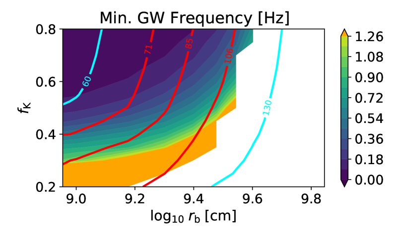
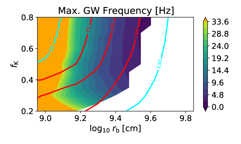
Figure 19: Mininum (top) and maximum (bottom) frequency of the predicted $l=m=2$ gravitational wave emission during the gravitationally unstable phase of collapsar accretion, for the same model shown in Fig. 9. Final BH mass contours are drawn as in previous figures.

We calculate the gravitational-wave strain of emitted gravitational waves by approximating ‘the lump’ of the unstable disk (assumed to correspond to an over-density of $\delta\rho/\rho\gtrsim 0.1$; Shibata et al. 2021; Wessel et al. 2021) and the central BH as two orbiting point masses. The frequencies of gravitational-wave emission can thus be directly predicted from the evolution of the disk angular velocity according to the collapsar model in Sec. 2.2. The maximum and minimum gravitational-wave frequencies vary considerably across the $\{f_{\rm K},r_{\rm b}\}$ parameter space (see Fig. 19 for our fiducial model).

According to the quadrupole formula, assuming that the orbital radius only slowly changes with respect to the orbital frequency, the plus ($h_{+}$) and cross ($h_{\times}$) polarizations of the gravitational waves at distance $r$ and inclination $\iota$ of the disk with respect to the observer can be written as

$$\mskip-20.0muh_{+}(t) = \frac{4G}{rc^{4}}\mu r_{\rm disk}^{2}\Omega_{\rm K,disk}^{2}\frac{1+\cos^{2}\iota}{2}\cos[\Phi(t)],$$ (E1)

$$\mskip-20.0muh_{\times}(t) = \frac{4G}{rc^{4}}\mu r_{\rm disk}^{2}\Omega_{\rm K,disk}^{2}\cos\iota\sin[\Phi(t)],$$ (E2)

where $\Phi(t)\equiv\int_{t_{0}}^{t}2\Omega_{\rm K,disk}(t^{\prime})\,\rm{d}t^{\prime}$, with $t=t_{0}$ denoting the start time of the gravitational instability. These expressions apply to the $l=m=2$ mode, while $\Omega_{\rm K,disk}$ is replaced by $0.5\Omega_{\rm K,disk}$ for the $m=1$ mode. Furthermore, $\mu=M_{\rm lump}M_{\bullet}/(M_{\rm lump}+M_{\bullet})$ is the reduced mass of the lump–BH system, and we set $M_{\rm lump}=f_{\rm lump}M_{\rm disk}$ with $f_{\rm lump}=0.2$. Uncertainties in the value of $f_{\rm lump}$ can be absorbed into uncertainties of the scale height of the disk and the threshold mass fraction $f_{\rm disk,thr}\equiv M_{\bullet}/M_{\rm disk}$ at which gravitational instabilities set in (cf. Eq. (25)). We neglect corrections $\propto\dot{\mu}$ to Eqs. (E1) and (E2) due to a time-dependent reduced mass $\mu$ as a result of accretion onto the black hole, assuming that $M_{\bullet}$ changes only weakly over the course of gravitational-wave emission.

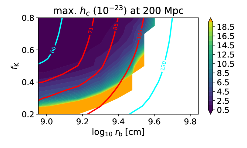
Figure 20: Maximum strain amplitude of the characteristic strain $h_{c}$ of gravitational waves from non-axisymmetric instabilities in self-gravitating collapsar disks across the parameter space of $\{r_{\rm b},f_{\rm K}\}$ for our fiducial model shown in Fig. 2 with $p=4.5$, $f_{\rm K}=0.3$ and $r_{\rm b}=1.5\times 10^{9}$ cm. Characteristic strains range from $\sim 10^{-24}-10^{-22}$ depending on the rotation profile of the progenitor. Final BH mass contours are drawn as in previous figures.

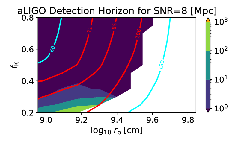
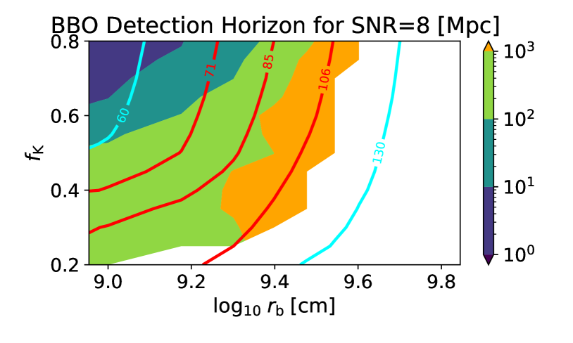
Figure 21: Detection horizons for gravitational waves from our fiducial model shown in Fig. 2 with $p=4.5$, $f_{\rm K}=0.3$ and $r_{\rm b}=1.5\times 10^{9}$ cm for advanced LIGO at design sensitivity (top) and Big Bang Observer (bottom), assuming optimal matched filtering and a signal-to-noise ratio of 8. While for aLIGO the detection horizon is typically limited to $\lesssim 100$ Mpc, BBO will be able to detect such sources up to typically several hundred Mpc to several Gpc, with particular sensitivity for progenitors with low-angular momentum ‘cores’ (medium to large values of $r_{\rm b}$). Contours delineate final BH masses as in previous figures.

We characterize gravitational-wave emission in the frequency domain (positive frequencies $f$ only) by computing the characteristic strain, defined as

$$h_{c}=2f|\tilde{h}^{\rm res}(f)|.$$ (E3)

For an estimate of the horizon distance we assume that the detector receives a signal from a directly overhead source and hence the optimal strain response at the detector can be written as

$$\tilde{h}^{\rm res}=\sqrt{|\tilde{h}_{+}|^{2}+|\tilde{h}_{\times}|^{2}},$$ (E4)

where $\tilde{h}_{+}$ and $\tilde{h}_{\times}$ are the Fourier transforms of the respective polarization strain amplitudes that we compute employing a Tukey window function limited to the physical frequencies between the maximum and minimum frequency expected from disk evolution (Fig. 19). We compare gravitational wave signals to detector sensitivity in terms of the amplitude spectral density $\sqrt{S_{h}}$ (Moore et al., 2015),

$$\sqrt{S_{h}}=2\sqrt{f}|\tilde{h}^{\rm res}|,$$ (E5)

where $S_{h}$ denotes the power spectral density, and calculate the signal-to-noise ratio (SNR) using an optimal filter (Moore et al., 2015),

$$\mathrm{SNR}=\left(\int df\frac{h_{c}^{2}}{S_{n}f^{2}}\right)^{\frac{1}{2}}.$$ (E6)

Characteristic strains of superKN collapsars range from $\sim 10^{-24}-10^{-22}$ depending on the rotation profile of the progenitor. A representative example is shown in Fig. 20. Detection horizons for advanced LIGO and BBO assuming $\text{SNR}=8$ are shown in Fig. 21, while those for CE, ET, and DECIGO are presented in Fig. 13.

Data Availability

The pre-collapse stellar models from Renzo et al. (2020b) and Heger et al. (2000), are available at https://zenodo.org/record/3406357 and https://2sn.org/stellarevolution/rotation/, respectively. Data of our model runs together with visualization scripts will be made available at https://doi.org/10.5281/zenodo.5639697.

References

- Abbott et al. (2020) Abbott, R., et al. 2020, Phys. Rev. Lett., 125, 101102, doi: 10.1103/PhysRevLett.125.101102
- Antonini & Rasio (2016) Antonini, F., & Rasio, F. A. 2016, ApJ, 831, 187, doi: 10.3847/0004-637X/831/2/187
- Aoki et al. (2014) Aoki, W., Tominaga, N., Beers, T. C., Honda, S., & Lee, Y. S. 2014, Science, 345, 912, doi: 10.1126/science.1252633
- Arnett (1982) Arnett, W. D. 1982, ApJ, 253, 785, doi: 10.1086/159681
- Arnould et al. (2007) Arnould, M., Goriely, S., & Takahashi, K. 2007, Phys. Rep., 450, 97, doi: 10.1016/j.physrep.2007.06.002
- Bardeen et al. (1972) Bardeen, J. M., Press, W. H., & Teukolsky, S. A. 1972, ApJ, 178, 347, doi: 10.1086/151796
- Barnes et al. (2018) Barnes, J., Duffell, P. C., Liu, Y., et al. 2018, ApJ, 860, 38, doi: 10.3847/1538-4357/aabf84
- Barnes & Kasen (2013) Barnes, J., & Kasen, D. 2013, Astrophys. J., 775, 18, doi: 10.1088/0004-637X/775/1/18
- Barnes et al. (2016) Barnes, J., Kasen, D., Wu, M.-R., & Martínez-Pinedo, G. 2016, ApJ, 829, 110, doi: 10.3847/0004-637X/829/2/110
- Barnes et al. (2021) Barnes, J., Zhu, Y. L., Lund, K. A., et al. 2021, ApJ, 918, 44, doi: 10.3847/1538-4357/ac0aec
- Bartos & Márka (2019) Bartos, I., & Márka, S. 2019, ApJ, 881, L4, doi: 10.3847/2041-8213/ab3215
- Belczynski et al. (2016) Belczynski, K., Holz, D. E., Bulik, T., & O’Shaughnessy, R. 2016, Nature, 534, 512, doi: 10.1038/nature18322
- Beloborodov (2003) Beloborodov, A. M. 2003, ApJ, 588, 931, doi: 10.1086/374217
- Berger (2014) Berger, E. 2014, Annu. Rev. Astron. Astrophys., 52, 43, doi: 10.1146/annurev-astro-081913-035926
- Blandford & Begelman (1999) Blandford, R. D., & Begelman, M. C. 1999, MNRAS, 303, L1, doi: 10.1046/j.1365-8711.1999.02358.x
- Bond et al. (1984) Bond, J. R., Arnett, W. D., & Carr, B. J. 1984, ApJ, 280, 825, doi: 10.1086/162057
- Bose et al. (2015) Bose, S., Valenti, S., Misra, K., et al. 2015, MNRAS, 450, 2373, doi: 10.1093/mnras/stv759
- Brauer et al. (2021) Brauer, K., Ji, A. P., Drout, M. R., & Frebel, A. 2021, ApJ, 915, 81, doi: 10.3847/1538-4357/ac00b2
- Bromberg et al. (2012) Bromberg, O., Nakar, E., Piran, T., & Sari, R. 2012, ApJ, 749, 110, doi: 10.1088/0004-637X/749/2/110
- Burbidge et al. (1957) Burbidge, E. M., Burbidge, G. R., Fowler, W. A., & Hoyle, F. 1957, Rev. Mod. Phys., 29, 547, doi: 10.1103/RevModPhys.29.547
- Callister et al. (2021) Callister, T. A., Farr, W. M., & Renzo, M. 2021, Astrophys. J., 920, 157, doi: 10.3847/1538-4357/ac1347
- Cameron (1957) Cameron, A. G. W. 1957, Publ. Astron. Soc. Pac., 69, 201, doi: 10.1086/127051
- Cano (2016) Cano, Z. 2016, in Eighth Huntsville Gamma-Ray Burst Symposium, Vol. 1962, 4116
- Cano et al. (2016) Cano, Z., Johansson Andreas, K. G., & Maeda, K. 2016, MNRAS, 457, 2761, doi: 10.1093/mnras/stw122
- Chen & Beloborodov (2007) Chen, W.-X., & Beloborodov, A. M. 2007, ApJ, 657, 383, doi: 10.1086/508923
- Christie et al. (2019) Christie, I. M., Lalakos, A., Tchekhovskoy, A., et al. 2019, Mon. Not. Roy. Astron. Soc., 490, 4811, doi: 10.1093/mnras/stz2552
- Costa et al. (2021) Costa, G., Bressan, A., Mapelli, M., et al. 2021, MNRAS, 501, 4514, doi: 10.1093/mnras/staa3916
- Côté et al. (2019) Côté, B., Eichler, M., Arcones, A., et al. 2019, ApJ, 875, 106, doi: 10.3847/1538-4357/ab10db
- Cowan et al. (2021) Cowan, J. J., Sneden, C., Lawler, J. E., et al. 2021, Reviews of Modern Physics, 93, 015002, doi: 10.1103/RevModPhys.93.015002
- Cowperthwaite et al. (2017) Cowperthwaite, P., Berger, E., Villar, V., et al. 2017, The Astrophysical Journal Letters, 848, L17
- Crowther et al. (2016) Crowther, P. A., Caballero-Nieves, S. M., Bostroem, K. A., et al. 2016, MNRAS, 458, 624, doi: 10.1093/mnras/stw273
- De & Siegel (2020) De, S., & Siegel, D. 2020, arXiv e-prints, 2011, arXiv:2011.07176. http://adsabs.harvard.edu/abs/2020arXiv201107176D
- de Koter et al. (1997) de Koter, A., Heap, S. R., & Hubeny, I. 1997, ApJ, 477, 792, doi: 10.1086/303736
- de Mink & Mandel (2016) de Mink, S. E., & Mandel, I. 2016, MNRAS, 460, 3545, doi: 10.1093/mnras/stw1219
- Delgado & Reuter (2016) Delgado, F., & Reuter, M. A. 2016, in Observatory Operations: Strategies, Processes, and Systems VI, Vol. 9910, International Society for Optics and Photonics, 991013
- Dessart et al. (2008) Dessart, L., Burrows, A., Livne, E., & Ott, C. D. 2008, ApJ, 673, L43, doi: 10.1086/527519
- Di Carlo et al. (2019) Di Carlo, U. N., Giacobbo, N., Mapelli, M., et al. 2019, MNRAS, 487, 2947, doi: 10.1093/mnras/stz1453
- Di Carlo et al. (2020) Di Carlo, U. N., Mapelli, M., Giacobbo, N., et al. 2020, MNRAS, 498, 495, doi: 10.1093/mnras/staa2286
- Di Matteo et al. (2002) Di Matteo, T., Perna, R., & Narayan, R. 2002, ApJ, 579, 706, doi: 10.1086/342832
- Dittmann et al. (2021) Dittmann, A. J., Cantiello, M., & Jermyn, A. S. 2021, ApJ, 916, 48, doi: 10.3847/1538-4357/ac042c
- Drout et al. (2017) Drout, M., Piro, A., Shappee, B., et al. 2017, Science, 358, 1570
- Duggan et al. (2018) Duggan, G. E., Kirby, E. N., Andrievsky, S. M., & Korotin, S. A. 2018, ApJ, 869, 50, doi: 10.3847/1538-4357/aaeb8e
- Eftekhari et al. (2020) Eftekhari, T., Berger, E., Margalit, B., Metzger, B. D., & Williams, P. K. G. 2020, ApJ, 895, 98, doi: 10.3847/1538-4357/ab9015
- Farmer et al. (2016) Farmer, R., Fields, C. E., Petermann, I., et al. 2016, ApJS, 227, 22, doi: 10.3847/1538-4365/227/2/22
- Farmer et al. (2020) Farmer, R., Renzo, M., de Mink, S. E., Fishbach, M., & Justham, S. 2020, ApJ, 902, L36, doi: 10.3847/2041-8213/abbadd
- Farmer et al. (2019) Farmer, R., Renzo, M., de Mink, S. E., Marchant, P., & Justham, S. 2019, ApJ, 887, 53, doi: 10.3847/1538-4357/ab518b
- Farrell et al. (2021) Farrell, E., Groh, J. H., Hirschi, R., et al. 2021, MNRAS, 502, L40, doi: 10.1093/mnrasl/slaa196
- Fernández et al. (2015) Fernández, R., Kasen, D., Metzger, B. D., & Quataert, E. 2015, Mon. Not. R. Astron. Soc., 446, 750, doi: 10.1093/mnras/stu2112
- Fernández & Metzger (2013) Fernández, R., & Metzger, B. D. 2013, Mon. Not. R. Astron. Soc., 435, 502, doi: 10.1093/mnras/stt1312
- Fernández et al. (2019) Fernández, R., Tchekhovskoy, A., Quataert, E., Foucart, F., & Kasen, D. 2019, MNRAS, 482, 3373, doi: 10.1093/mnras/sty2932
- Fishbach & Holz (2020) Fishbach, M., & Holz, D. E. 2020, ApJ, 904, L26, doi: 10.3847/2041-8213/abc827
- Fruchter et al. (2006) Fruchter, A. S., et al. 2006, Nature, 441, 463, doi: 10.1038/nature04787
- Fujibayashi et al. (2018) Fujibayashi, S., Kiuchi, K., Nishimura, N., Sekiguchi, Y., & Shibata, M. 2018, ApJ, 860, 64, doi: 10.3847/1538-4357/aabafd
- Fujibayashi et al. (2020) Fujibayashi, S., Shibata, M., Wanajo, S., et al. 2020, Phys. Rev. D, 101, 083029, doi: 10.1103/PhysRevD.101.083029
- Fujibayashi et al. (2021) Fujibayashi, S., Takahashi, K., Sekiguchi, Y., & Shibata, M. 2021, arXiv e-prints, arXiv:2102.04467. https://arxiv.org/abs/2102.04467
- Fuller & Ma (2019) Fuller, J., & Ma, L. 2019, ApJ, 881, L1, doi: 10.3847/2041-8213/ab339b
- Fynbo et al. (2006) Fynbo, J. P. U., Watson, D., Thöne, C. C., et al. 2006, Nature, 444, 1047, doi: 10.1038/nature05375
- Gall et al. (2017) Gall, C., Hjorth, J., Rosswog, S., Tanvir, N. R., & Levan, A. J. 2017, ApJ, 849, L19, doi: 10.3847/2041-8213/aa93f9
- Gammie (2001) Gammie, C. F. 2001, ApJ, 553, 174, doi: 10.1086/320631
- Gehrels et al. (2006) Gehrels, N., Norris, J. P., Barthelmy, S. D., et al. 2006, Nature, 444, 1044, doi: 10.1038/nature05376
- Gerosa & Fishbach (2021) Gerosa, D., & Fishbach, M. 2021, Nature Astronomy, 5, 749, doi: 10.1038/s41550-021-01398-w
- Glatzel et al. (1985) Glatzel, W., Fricke, K. J., & El Eid, M. F. 1985, A&A, 149, 413
- Goldstein et al. (2016) Goldstein, A., Connaughton, V., Briggs, M. S., & Burns, E. 2016, ApJ, 818, 18, doi: 10.3847/0004-637X/818/1/18
- Gottlieb et al. (2021) Gottlieb, O., Lalakos, A., Bromberg, O., Liska, M., & Tchekhovskoy, A. 2021, arXiv e-prints, arXiv:2109.14619. https://arxiv.org/abs/2109.14619
- Graham et al. (2020) Graham, M. J., Ford, K. E. S., McKernan, B., et al. 2020, Phys. Rev. Lett., 124, 251102, doi: 10.1103/PhysRevLett.124.251102
- Grichener & Soker (2019) Grichener, A., & Soker, N. 2019, ApJ, 878, 24, doi: 10.3847/1538-4357/ab1d5d
- Heger et al. (2000) Heger, A., Langer, N., & Woosley, S. E. 2000, Astrophys. J., 528, 368, doi: 10.1086/308158
- Hiramatsu et al. (2021) Hiramatsu, D., Howell, D. A., Van Dyk, S. D., et al. 2021, Nature Astronomy, 5, 903, doi: 10.1038/s41550-021-01384-2
- Holmbeck et al. (2019) Holmbeck, E. M., Frebel, A., McLaughlin, G. C., et al. 2019, ApJ, 881, 5, doi: 10.3847/1538-4357/ab2a01
- Horowitz et al. (2019) Horowitz, C. J., Arcones, A., Côté, B., et al. 2019, Journal of Physics G Nuclear Physics, 46, 083001, doi: 10.1088/1361-6471/ab0849
- Hotokezaka et al. (2015) Hotokezaka, K., Piran, T., & Paul, M. 2015, Nature Physics, 11, 1042, doi: 10.1038/nphys3574
- Hotokezaka et al. (2021) Hotokezaka, K., Tanaka, M., Kato, D., & Gaigalas, G. 2021, arXiv e-prints, arXiv:2102.07879. https://arxiv.org/abs/2102.07879
- Janiuk et al. (2004) Janiuk, A., Perna, R., Di Matteo, T., & Czerny, B. 2004, MNRAS, 355, 950, doi: 10.1111/j.1365-2966.2004.08377.x
- Japelj et al. (2018) Japelj, J., Vergani, S. D., Salvaterra, R., et al. 2018, A&A, 617, A105, doi: 10.1051/0004-6361/201833209
- Jermyn et al. (2021) Jermyn, A. S., Dittmann, A. J., Cantiello, M., & Perna, R. 2021, Astrophys. J., 914, 105, doi: 10.3847/1538-4357/abfb67
- Ji et al. (2016) Ji, A. P., Frebel, A., Chiti, A., & Simon, J. D. 2016, Nature, 531, 610, doi: 10.1038/nature17425
- Jin et al. (2015) Jin, Z.-P., Li, X., Cano, Z., et al. 2015, The Astrophysical Journal Letters, 811, L22
- Just et al. (2015) Just, O., Bauswein, A., Pulpillo, R. A., Goriely, S., & Janka, H.-T. 2015, Mon. Not. R. Astron. Soc., 448, 541, doi: 10.1093/mnras/stv009
- Just et al. (2021) Just, O., Goriely, S., Janka, H.-T., Nagataki, S., & Bauswein, A. 2021, arXiv:2102.08387. http://arxiv.org/abs/2102.08387
- Kalogera (1996) Kalogera, V. 1996, ApJ, 471, 352, doi: 10.1086/177974
- Kasen et al. (2013) Kasen, D., Badnell, N. R., & Barnes, J. 2013, ApJ, submitted, arXiv:1303.5788. https://arxiv.org/abs/1303.5788
- Kasen et al. (in prep.) Kasen, D., Roth, N., Klion, H., Khatami, D., & Tsang, B. in prep.
- Kasen et al. (2006) Kasen, D., Thomas, R. C., & Nugent, P. 2006, ApJ, 651, 366, doi: 10.1086/506190
- Kasliwal et al. (2017) Kasliwal, M. M., Bally, J., et al. 2017, ApJ, 839, 88, doi: 10.3847/1538-4357/aa6978
- Khatami & Kasen (2019) Khatami, D. K., & Kasen, D. N. 2019, ApJ, 878, 56, doi: 10.3847/1538-4357/ab1f09
- Kiuchi, K. et al. (2011) Kiuchi, K., Yoshida, S., & Shibata, M. 2011, A&A, 532, A30, doi: 10.1051/0004-6361/201016242
- Kumar et al. (2008) Kumar, P., Narayan, R., & Johnson, J. L. 2008, MNRAS, 388, 1729, doi: 10.1111/j.1365-2966.2008.13493.x
- Langer (1998) Langer, N. 1998, A&A, 329, 551
- Lattimer & Schramm (1974) Lattimer, J. M., & Schramm, D. N. 1974, Astrophys. J. Lett., 192, L145, doi: 10.1086/181612
- Li & Paczyński (1998) Li, L.-X., & Paczyński, B. 1998, Astrophys. J. Lett., 507, L59, doi: 10.1086/311680
- Li & Siegel (2021) Li, X., & Siegel, D. M. 2021, Phys. Rev. Lett., 126, 251101, doi: 10.1103/PhysRevLett.126.251101
- Liang et al. (2007) Liang, E., Zhang, B., Virgili, F., & Dai, Z. G. 2007, ApJ, 662, 1111, doi: 10.1086/517959
- Lippuner & Roberts (2015) Lippuner, J., & Roberts, L. F. 2015, Astrophys. J., 815, 82, doi: 10.1088/0004-637X/815/2/82
- Ma & Fuller (2019) Ma, L., & Fuller, J. 2019, MNRAS, 488, 4338, doi: 10.1093/mnras/stz2009
- MacFadyen & Woosley (1999) MacFadyen, A. I., & Woosley, S. E. 1999, ApJ, 524, 262, doi: 10.1086/307790
- Macias & Ramirez-Ruiz (2019) Macias, P., & Ramirez-Ruiz, E. 2019, ApJ, 877, L24, doi: 10.3847/2041-8213/ab2049
- Maeder & Meynet (2000) Maeder, A., & Meynet, G. 2000, ARA&A, 38, 143, doi: 10.1146/annurev.astro.38.1.143
- Mandel & de Mink (2016) Mandel, I., & de Mink, S. E. 2016, MNRAS, 458, 2634, doi: 10.1093/mnras/stw379
- Mandel & Fragos (2020) Mandel, I., & Fragos, T. 2020, ApJ, 895, L28, doi: 10.3847/2041-8213/ab8e41
- Marchant et al. (2016) Marchant, P., Langer, N., Podsiadlowski, P., Tauris, T. M., & Moriya, T. J. 2016, A&A, 588, A50, doi: 10.1051/0004-6361/201628133
- Marchant & Moriya (2020) Marchant, P., & Moriya, T. J. 2020, A&A, 640, L18, doi: 10.1051/0004-6361/202038902
- Marchant et al. (2019) Marchant, P., Renzo, M., Farmer, R., et al. 2019, ApJ, 882, 36, doi: 10.3847/1538-4357/ab3426
- Margutti & Chornock (2020) Margutti, R., & Chornock, R. 2020, arXiv e-prints, arXiv:2012.04810. https://arxiv.org/abs/2012.04810
- Mehta et al. (2021) Mehta, A. K., Buonanno, A., Gair, J., et al. 2021, arXiv e-prints, arXiv:2105.06366. https://arxiv.org/abs/2105.06366
- Metzger (2019) Metzger, B. D. 2019, Living Reviews in Relativity, 23, 1, doi: 10.1007/s41114-019-0024-0
- Metzger & Bower (2014) Metzger, B. D., & Bower, G. C. 2014, MNRAS, 437, 1821, doi: 10.1093/mnras/stt2010
- Metzger et al. (2008) Metzger, B. D., Piro, A. L., & Quataert, E. 2008, MNRAS, 390, 781, doi: 10.1111/j.1365-2966.2008.13789.x
- Metzger et al. (2007) Metzger, B. D., Thompson, T. A., & Quataert, E. 2007, Astrophys. J., 659, 561, doi: 10.1086/512059
- Metzger et al. (2008) Metzger, B. D., Thompson, T. A., & Quataert, E. 2008, Astrophys. J., 676, 1130, doi: 10.1086/526418
- Metzger et al. (2015) Metzger, B. D., Williams, P. K. G., & Berger, E. 2015, ApJ, 806, 224, doi: 10.1088/0004-637X/806/2/224
- Metzger et al. (2010) Metzger, B. D., Martínez-Pinedo, G., Darbha, S., et al. 2010, Mon. Not. R. Astron. Soc., 406, 2650, doi: 10.1111/j.1365-2966.2010.16864.x
- Miller et al. (2020) Miller, J. M., Sprouse, T. M., Fryer, C. L., et al. 2020, ApJ, 902, 66, doi: 10.3847/1538-4357/abb4e3
- Modjaz et al. (2020) Modjaz, M., Bianco, F. B., Siwek, M., et al. 2020, ApJ, 892, 153, doi: 10.3847/1538-4357/ab4185
- Moore et al. (2015) Moore, C. J., Cole, R. H., & Berry, C. P. L. 2015, Class. Quantum Grav. , 32, 015014, doi: 10.1088/0264-9381/32/1/015014
- Nakar (2020) Nakar, E. 2020, Phys. Rep., 886, 1, doi: 10.1016/j.physrep.2020.08.008
- Nakar & Piran (2011) Nakar, E., & Piran, T. 2011, Nature, 478, 82, doi: 10.1038/nature10365
- Narayana Bhat et al. (2016) Narayana Bhat, P., Meegan, C. A., von Kienlin, A., et al. 2016, ApJS, 223, 28, doi: 10.3847/0067-0049/223/2/28
- Nishimura et al. (2015) Nishimura, N., Takiwaki, T., & Thielemann, F.-K. 2015, ApJ, 810, 109, doi: 10.1088/0004-637X/810/2/109
- Nitz & Capano (2021) Nitz, A. H., & Capano, C. D. 2021, ApJ, 907, L9, doi: 10.3847/2041-8213/abccc5
- Ofek (2017) Ofek, E. O. 2017, ApJ, 846, 44, doi: 10.3847/1538-4357/aa8310
- Paczynski (1978) Paczynski, B. 1978, Acta Astron., 28, 91. http://adsabs.harvard.edu/pdf/1978AcA....28...91P7
- Pedregosa et al. (2011) Pedregosa, F., Varoquaux, G., Gramfort, A., et al. 2011, Journal of Machine Learning Research, 12, 2825
- Perna et al. (2021) Perna, R., Lazzati, D., & Cantiello, M. 2021, ApJ, 906, L7, doi: 10.3847/2041-8213/abd319
- Pescalli et al. (2016) Pescalli, A., Ghirlanda, G., Salvaterra, R., et al. 2016, A&A, 587, A40, doi: 10.1051/0004-6361/201526760
- Petrosian et al. (2015) Petrosian, V., Kitanidis, E., & Kocevski, D. 2015, ApJ, 806, 44, doi: 10.1088/0004-637X/806/1/44
- Powell et al. (2021) Powell, J., Müller, B., & Heger, A. 2021, MNRAS, 503, 2108, doi: 10.1093/mnras/stab614
- Qian & Woosley (1996) Qian, Y.-Z., & Woosley, S. E. 1996, ApJ, 471, 331, doi: 10.1086/177973
- Raynaud et al. (2020) Raynaud, R., Guilet, J., Janka, H.-T., & Gastine, T. 2020, Science Advances, 6, eaay2732, doi: 10.1126/sciadv.aay2732
- Reichert et al. (2021) Reichert, M., Hansen, C. J., & Arcones, A. 2021, ApJ, 912, 157, doi: 10.3847/1538-4357/abefd8
- Renzo et al. (2020a) Renzo, M., Cantiello, M., Metzger, B. D., & Jiang, Y. F. 2020a, ApJ, 904, L13, doi: 10.3847/2041-8213/abc6a6
- Renzo et al. (2020b) Renzo, M., Farmer, R., Justham, S., et al. 2020b, A&A, 640, A56, doi: 10.1051/0004-6361/202037710
- Roberts et al. (2010) Roberts, L. F., Woosley, S. E., & Hoffman, R. D. 2010, ApJ, 722, 954, doi: 10.1088/0004-637X/722/1/954
- Safarzadeh & Haiman (2020) Safarzadeh, M., & Haiman, Z. 2020, ApJ, 903, L21, doi: 10.3847/2041-8213/abc253
- Schlegel et al. (1998) Schlegel, D. J., Finkbeiner, D. P., & Davis, M. 1998, The Astrophysical Journal, 500, 525
- Schneider et al. (2018) Schneider, F. R. N., Sana, H., Evans, C. J., et al. 2018, Science, 359, 69, doi: 10.1126/science.aan0106
- Schroeder et al. (2020) Schroeder, G., Margalit, B., Fong, W.-f., et al. 2020, ApJ, 902, 82, doi: 10.3847/1538-4357/abb407
- Shakura & Sunyaev (1973) Shakura, N. I., & Sunyaev, R. A. 1973, A&A, 24, 337. http://adsabs.harvard.edu/abs/1973A%26A....24..337S
- Shankar et al. (2021) Shankar, S., Mösta, P., Barnes, J., Duffell, P. C., & Kasen, D. 2021, arXiv e-prints, arXiv:2105.08092. https://arxiv.org/abs/2105.08092
- Shapiro & Teukolsky (1983) Shapiro, S. L., & Teukolsky, S. A. 1983, Black Holes, White Dwarfs, and Neutron Stars (New York: John Wiley & Sons)
- Shen et al. (2015) Shen, S., Cooke, R. J., Ramirez-Ruiz, E., et al. 2015, Astrophys. J., 807, 115, doi: 10.1088/0004-637X/807/2/115
- Shibata et al. (2021) Shibata, M., Kiuchi, K., Fujibayashi, S., & Sekiguchi, Y. 2021, Phys. Rev. D, 103, 063037, doi: 10.1103/PhysRevD.103.063037
- Siegel (2019) Siegel, D. M. 2019, European Physical Journal A, 55, 203, doi: 10.1140/epja/i2019-12888-9
- Siegel (2021) Siegel, D. M. 2021, Nat. Rev. Phys., submitted
- Siegel et al. (2019) Siegel, D. M., Barnes, J., & Metzger, B. D. 2019, Nature, 569, 241, doi: 10.1038/s41586-019-1136-0
- Siegel & Metzger (2017) Siegel, D. M., & Metzger, B. D. 2017, Phys. Rev. Lett., 119, 231102, doi: 10.1103/PhysRevLett.119.231102
- Siegel & Metzger (2018) —. 2018, ApJ, 858, 52, doi: 10.3847/1538-4357/aabaec
- Smith et al. (2007) Smith, N., Li, W., Foley, R. J., et al. 2007, ApJ, 666, 1116, doi: 10.1086/519949
- Sobacchi et al. (2017) Sobacchi, E., Granot, J., Bromberg, O., & Sormani, M. C. 2017, MNRAS, 472, 616, doi: 10.1093/mnras/stx2083
- Spergel et al. (2015) Spergel, D., Gehrels, N., Baltay, C., et al. 2015, arXiv e-prints, arXiv:1503.03757. https://arxiv.org/abs/1503.03757
- Spruit (2002) Spruit, H. C. 2002, A&A, 381, 923, doi: 10.1051/0004-6361:20011465
- Sun et al. (2015) Sun, H., Zhang, B., & Li, Z. 2015, ApJ, 812, 33, doi: 10.1088/0004-637X/812/1/33
- Surman et al. (2006) Surman, R., McLaughlin, G. C., & Hix, W. R. 2006, ApJ, 643, 1057, doi: 10.1086/501116
- Surman et al. (2008) Surman, R., McLaughlin, G. C., Ruffert, M., Janka, H.-T., & Hix, W. R. 2008, Astrophys. J. Lett., 679, L117, doi: 10.1086/589507
- Symbalisty & Schramm (1982) Symbalisty, E., & Schramm, D. N. 1982, Astrophys. J. Lett., 22, 143
- Tagawa et al. (2021) Tagawa, H., Haiman, Z., Bartos, I., Kocsis, B., & Omukai, K. 2021, MNRAS, 507, 3362, doi: 10.1093/mnras/stab2315
- Takami et al. (2014) Takami, H., Nozawa, T., & Ioka, K. 2014, ApJ, 789, L6, doi: 10.1088/2041-8205/789/1/L6
- Tanaka & Hotokezaka (2013) Tanaka, M., & Hotokezaka, K. 2013, Astrophys. J., 775, 113, doi: 10.1088/0004-637X/775/2/113
- Tanaka et al. (2020) Tanaka, M., Kato, D., Gaigalas, G., & Kawaguchi, K. 2020, MNRAS, 496, 1369, doi: 10.1093/mnras/staa1576
- Tarumi et al. (2021) Tarumi, Y., Hotokezaka, K., & Beniamini, P. 2021, Astrophys. J. Lett., 913, L30, doi: 10.3847/2041-8213/abfe13
- Thompson & Duncan (1993) Thompson, C., & Duncan, R. C. 1993, ApJ, 408, 194, doi: 10.1086/172580
- Thompson et al. (2004) Thompson, T. A., Chang, P., & Quataert, E. 2004, Astrophys. J., 611, 380, doi: 10.1086/421969
- Tomita et al. (2006) Tomita, H., Deng, J., Maeda, K., et al. 2006, ApJ, 644, 400, doi: 10.1086/503554
- Tsujimoto et al. (2017) Tsujimoto, T., Matsuno, T., Aoki, W., Ishigaki, M. N., & Shigeyama, T. 2017, ApJ, 850, L12, doi: 10.3847/2041-8213/aa9886
- Tsvetkov et al. (2013) Tsvetkov, D. Y., Shugarov, S. Y., Volkov, I. M., et al. 2013, Contributions of the Astronomical Observatory Skalnate Pleso, 43, 94. https://arxiv.org/abs/1311.3484
- Tyson (2002) Tyson, J. A. 2002, in Society of Photo-Optical Instrumentation Engineers (SPIE) Conference Series, Vol. 4836, Survey and Other Telescope Technologies and Discoveries, ed. J. A. Tyson & S. Wolff, 10–20, doi: 10.1117/12.456772
- van de Voort et al. (2020) van de Voort, F., Pakmor, R., Grand, R. J. J., et al. 2020, MNRAS, 494, 4867, doi: 10.1093/mnras/staa754
- van den Heuvel et al. (2017) van den Heuvel, E. P. J., Portegies Zwart, S. F., & de Mink, S. E. 2017, MNRAS, 471, 4256, doi: 10.1093/mnras/stx1430
- van Son et al. (2021) van Son, L. A. C., de Mink, S. E., Callister, T., et al. 2021, arXiv e-prints, arXiv:2110.01634. https://arxiv.org/abs/2110.01634
- Villar et al. (2017) Villar, V. A., Guillochon, J., Berger, E., et al. 2017, ApJ, 851, L21, doi: 10.3847/2041-8213/aa9c84
- Vink et al. (2021) Vink, J. S., Higgins, E. R., Sander, A. A. C., & Sabhahit, G. N. 2021, MNRAS, 504, 146, doi: 10.1093/mnras/stab842
- Wallner et al. (2015) Wallner, A., Faestermann, T., Feige, J., et al. 2015, Nature Commun., 6, 5956, doi: 10.1038/ncomms6956
- Wanderman & Piran (2010) Wanderman, D., & Piran, T. 2010, MNRAS, no, doi: 10.1111/j.1365-2966.2010.16787.x
- Wessel et al. (2021) Wessel, E., Paschalidis, V., Tsokaros, A., Ruiz, M., & Shapiro, S. L. 2021, Physical Review D, 103, 043013, doi: 10.1103/PhysRevD.103.043013
- Winteler et al. (2012) Winteler, C., Käppeli, R., Perego, A., et al. 2012, Astrophys. J. Lett., 750, L22, doi: 10.1088/2041-8205/750/1/L22
- Woosley (2017) Woosley, S. E. 2017, ApJ, 836, 244, doi: 10.3847/1538-4357/836/2/244
- Woosley & Bloom (2006) Woosley, S. E., & Bloom, J. S. 2006, ARA&A, 44, 507, doi: 10.1146/annurev.astro.43.072103.150558
- Woosley & Heger (2006) Woosley, S. E., & Heger, A. 2006, ApJ, 637, 914, doi: 10.1086/498500
- Woosley & Heger (2021) Woosley, S. E., & Heger, A. 2021, Astrophys. J. Lett., 912, L31, doi: 10.3847/2041-8213/abf2c4
- Woosley et al. (2002) Woosley, S. E., Heger, A., & Weaver, T. A. 2002, Rev. Mod. Phys., 74, 1015, doi: 10.1103/RevModPhys.74.1015
- Woosley & Hoffman (1992) Woosley, S. E., & Hoffman, R. D. 1992, ApJ, 395, 202, doi: 10.1086/171644
- Yagi & Seto (2011) Yagi, K., & Seto, N. 2011, Physical Review D, 83, doi: 10.1103/physrevd.83.044011
- Yamazaki et al. (2021) Yamazaki, Y., Kajino, T., Mathews, G. J., et al. 2021, arXiv e-prints, arXiv:2102.05891. https://arxiv.org/abs/2102.05891
- Yang et al. (2019) Yang, Y., Bartos, I., Gayathri, V., et al. 2019, Phys. Rev. Lett., 123, 181101, doi: 10.1103/PhysRevLett.123.181101
- Yüksel et al. (2008) Yüksel, H., Kistler, M. D., Beacom, J. F., & Hopkins, A. M. 2008, ApJ, 683, L5, doi: 10.1086/591449
- Zenati et al. (2020) Zenati, Y., Siegel, D. M., Metzger, B. D., & Perets, H. B. 2020, MNRAS, 499, 4097, doi: 10.1093/mnras/staa3002
- Zhang et al. (2007) Zhang, B., Zhang, B.-B., Liang, E.-W., et al. 2007, ApJ, 655, L25, doi: 10.1086/511781