Model-free based control of a HIV/AIDS prevention model

Abstract

Controlling an epidemiological model is often performed using optimal control theory techniques for which the solution depends on the equations of the control system, objective functional and possible state and/or control constraints. In this paper, we propose a model-free control approach based on an algorithm that operates in ’real-time’ and drives the state solution according to a direct feedback on the state solution that is aimed to be minimized, and without knowing explicitly the equations of the control system. We consider a concrete epidemic problem of minimizing the number of HIV infected individuals, through the preventive measure pre-exposure prophylaxis (PrEP) given to susceptible individuals. The solutions must satisfy control and mixed state-control constraints that represent the limitations on PrEP implementation. Our model-free based control algorithm allows to close the loop between the number of infected individuals with HIV and the supply of PrEP medication ’in real time’, in such manner that the number of infected individuals is asymptotically reduced and the number of individuals under PrEP medication is below a fixed constant value. We prove the efficiency of our approach and compare the model-free control solutions with the ones obtained using a classical optimal control approach via Pontryagin maximum principle. The performed numerical simulations allow us to conclude that the model-free based control strategy highlights new and interesting performances compared with the classical optimal control approach.

1 Introduction

The SICA (Susceptible–Infected–Chronic–AIDS) compartmental model for HIV/AIDS transmission dynamics was proposed by Silva and Torres in their seminal paper [21]. Since then, the model has been extended to stochastic systems of differential equations [6, 28], to fractional-order [24, 30] as well as discrete-time dynamics [27], and applied with success to describe very different HIV/AIDS epidemics, like the ones in Cape Verde [22, 23] or Morocco [14]. For a survey see [25].

In this work, we consider a SICA epidemic problem of controlling the transmission of the human immunodeficiency viruses (HIV), by considering not only the medical treatment with multiple antiretroviral (ART) drugs, but also the pre-exposure prophylaxis (PrEP), which are medicines taken to prevent getting HIV infection. According to the Centers for Disease Control and Prevention, PrEP is highly effective for preventing HIV, when taken as prescribed, and reduces the risk of getting HIV from sex and from injection drug use by about 99% and 74%, respectively [4].

The main contribution of this work is to propose a model-free based control algorithm that closes the loop between the infected individuals with HIV and PreP medication, in such manner that the medication is driven in ’real-time’, according to the number of infected individuals that has to be asymptotically reduced. We highlight that model-free control offers the advantages of a simple Proportional–Integral–Derivative (PID) controller in the framework of model free design, that is, one whose parameters that can be easily tuned without a precise knowledge of the controlled epidemiological model.

The model-free control methodology, originally proposed by Fliess and Join in [10], has been designed to control a priori any “unknown” dynamical system in a “robust” manner, and is referred to as “a self-tuning regulator” in [1]. This control law can be considered as an alternative to PI and PID controllers [11] and the performances are really satisfactory taking into account that the control is calculated based only on the information provided by the controlled input and the measured output signal of the controlled systems. This control law has been extensively and successfully applied to control many nonlinear processes: see, e.g., [3, 10, 12] and the references therein. In particular, some applications have been dedicated to the control of chemistry and biological processes [2, 3, 13, 17, 26], including the development of an artificial pancreas [16]. A derivative-free-based version of this control algorithm has been proposed by the first author in [15], for which some interesting capabilities of online optimization have been highlighted. To the best of our knowledge, the application of model-free control to SICA modeling has never been discussed before.

Here, we compare the solutions obtained by the model-free control method with the corresponding solutions of an optimal control problem for HIV/AIDS transmission from [23], which has a mixed state-control constraint. In [23], the control system is based on a SICAE (Susceptible, HIV-Infected, Chronic HIV-infected under ART, AIDS-symptomatic individuals, E – under PrEP medication) model for the transmission of HIV in a homogeneously mixing population. The control $u$ represents the fraction of susceptible individuals under PrEP, with $0\leq u(t)\leq 1$, that is, when $u(t)=0$, no susceptible individual takes PrEP at time $t$, and when $u(t)=1$ all susceptible individuals are taking PrEP at time $t$. The mixed state-control constraint refers to the fact that only people who are HIV-negative and at a very high risk of HIV infection should take PrEP, and also to the high costs of PrEP medication. Therefore, the number of susceptible individuals that takes PrEP, at each day, must be bounded by a positive constant. Moreover, the cost functional, which is aimed to be minimized, represents a balance between the number of HIV infected individuals and the costs associated with PrEP implementation.

The paper is structured as follows. In Section 2, we propose a model-free control method and the procedure to minimize the HIV infected cases is described. In Section 3, we present some numerical simulations and provide a comparison of the results obtained using the model-free based approach with the ones in [23] from the Pontryagin maximum principle. Section 4 discusses and compares the results. Finally, some concluding remarks and possible directions for future work are given in Section 5.

2 Materials and methods

In this section, we propose our model-free based control method and apply it to an epidemiological problem of minimizing HIV-infected individuals.

2.1 Principle of the model-free based control

Model-free based control was introduced in 2008 and 2009 by Fliess and Join in [8, 9]. It is an alternative technique to control complex systems based on elementary continuously updated local modeling via unique knowledge of the input-output behavior. The key feature of this approach lies in the fact that the control system, which might be highly nonlinear and/or time-varying, is taken into account without any modeling procedure [18]. The model-free based control approach has been successfully implemented in concrete applications to diverse fields, ranging from intelligent transportation systems to energy management, etc., see [10] and references cited therein. To the best of our knowledge, no one as yet used this approach in the context of epidemiology.

Consider a nonlinear dynamical system $f:u\mapsto y$ to control:

$$\left\{\begin{array}[]{l}\dot{\boldsymbol{x}}=f(\boldsymbol{x},u),\\ y=g(\boldsymbol{x}),\end{array}\right.$$ (2.1)

where $f$ is the function describing the behavior of a nonlinear system and $\boldsymbol{x}\in\mathbb{R}$ is the state vector. The para-model control is an application $\mathcal{C}_{\pi}:(y,y^{*})\mapsto u$, whose purpose is to control the output $y$ of (2.1) following an output reference $y^{*}$. In simulation, the system (2.1) is controlled in its “original formulation”, without any modification or linearization.

For any discrete moment $t_{k},\,k\in\mathbb{N}^{*}$, one defines the discrete controller $\mathcal{C}_{\pi}:(y,y^{*})\mapsto u$ as an integrator associated to a numerical series $(\Psi_{k})_{k\in\mathbb{Z}}$, symbolically represented by

$$u_{k}=\mathcal{C}_{\pi}(y_{k},y^{*}_{k})=\Psi_{k}\cdot\int_{0}^{t}K_{i}(y^{\ast}_{k}-y_{k-1})\,d\,\tau$$ (2.2)

with the recursive term

$$\Psi_{k}=\Psi_{k-1}+{K_{p}}(k_{\alpha}e^{-k_{\beta}k}-y_{k-1}),$$

where $y^{\ast}$ is the output (or tracking) reference trajectory; $K_{p}$ and $K_{i}$ are real positive tuning gains; $\varepsilon_{k-1}=y^{\ast}_{k}-y_{k-1}$ is the tracking error; and $k_{\alpha}e^{-k_{\beta}k}$ is an initialization function, where $k_{\alpha}$ and $k_{\beta}$ are real positive constants. In practice, the integral part is discretized using, for example, Riemann sums.

The set of the $\mathcal{C}_{\pi}$-parameters of the controller, is defined as the set of the tuning coefficients $\{K_{p},K_{i},k_{\alpha},k_{\beta}\}$.

2.2 Methodology

Consider the problem of minimizing the number of infected individuals with HIV, given by the state trajectory $I$, through the control measure $u$ associated to PrEP medication, and satisfying a mixed state-control constraint $Su\leq\eta$, where $\eta$ is a positive constant.

The control sequence is divided into two steps, in order to manage, separately, the increasing $u$ transient and the associated decreasing $u$ transient that must decrease afterwards both the infected cases and the control input $u$ to lower values on $u$ and $I$. Concerning the control input $u$, it is expected that $u(t>t_{f})=0$, where $t_{f}$ is the time from which the medication is stopped.

• A first sequence, associated to the setting up of the medication, aims to progressively increase the medication (and thus start decreasing the infected states) until a certain threshold of infected cases is reached, above which the number of infected cases could be considered as stabilizable around a low value. This control sequence can be managed by a simple $L$-linear or $Q$-quadratic slope, such as

  $$\mathrm{(slope)}\quad u(t)=u_{0}+L\cdot t\qquad\qquad\mathrm{(quadratic)}\quad u(t)=u_{0}+Q\cdot t^{2}$$ (2.3)

  driven in open-loop, i.e., independently from any feedback of the infected state, that increases gradually the medication while satisfying the constraint on $Su\leq\eta$ due to the remaining high level of the susceptible cases. It appears crucial to accelerate the medication at the beginning, in order to reach rapidly $\gamma_{lim}$ and allow a strong decreasing of the infected cases. This point will be discussed later in Section 3.

• Denote $u_{max}=\max u(t)$, the maximum value of $u$. The second sequence is associated to the decrease of the medication until the infected state is stabilized around a low value. This sequence is managed by our proposed model-free based control that interacts, in real-time, with the number of infected cases and, consequently, calculates the “optimal” medication $u$ in order to decrease and stabilize the infected state. According to (2.2), the control reads:

  $$u_{k}=\Psi_{k}\,\cdot\int_{0}^{t}K_{i}(I^{\ast}_{k}-I_{k-1})\,d\,\tau\qquad\mathrm{with}\qquad\Psi_{k}=\Psi_{k-1}+{K_{p}}(k_{\alpha}e^{-k_{\beta}k}-I_{k-1}),$$

  where $I^{\ast}$ denotes the infected cases reference that practically can be chosen as $I^{\ast}=\min I(t)$, where the minimum value of $I$ can be reached online, updating the tracking reference and, therefore, ensuring that the control law is “synchronized” on the lowest value that can be reachable. It is worth to note that, depending on the behavior of the closed-loop, a saturation is added to bound the controlled $u$: $0\leq u\leq u_{max}\leq 1$.

The implementation of the control scheme is depicted in Figure 1, where the control sequence starts from the transient slope or the quadratic function and then, once $u_{max}$ is reached, switches to the proposed model-free based controller. The parameters of the control sequence to be adjusted, comprise the $\mathcal{C}_{\pi}$-parameters set of the model-free control algorithm and the $(u_{0},L,Q)$ parameters of the first sequence, depending if a linear or a quadratic slope is involved.

Additional constraints.

The slope can be adjusted according to a state-control constraint that determines the maximum number of susceptible individuals that take PrEP medication, at each instant of time. This constraint reads as $S(t)\cdot u(t)<\gamma_{max}$, for all $t$, where $\gamma_{max}$ is the corresponding upper bound.

To properly tune each sequence, in order to satisfy both the state-control constraint as well as to minimize the cost criteria, a derivative-free based optimization procedure can be applied [19].

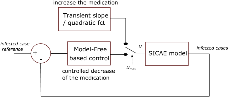
Figure 1: Proposed scheme to control a nonlinear system.

2.3 Classical optimal control problem applied to the HIV/AIDS SICAE model with a mixed state-control constraint

Consider the mathematical model for HIV/AIDS transmission in a homogeneously mixing population proposed in [23] and based in [21, 22].

The model subdivides human population into five mutually-exclusive compartments: susceptible individuals ($S$); HIV-infected individuals with no clinical symptoms of AIDS (the virus is living or developing in the individuals but without producing symptoms or only mild ones) but able to transmit HIV to other individuals ($I$); HIV-infected individuals under ART treatment (the so called chronic stage) with a viral load remaining low ($C$); HIV-infected individuals with AIDS clinical symptoms ($A$); individuals that are under PrEP medication ($E$). The total population at time $t$, denoted by $N(t)$, is given by $N(t)=S(t)+I(t)+C(t)+A(t)+E(t)$. The model assumptions are the following [21, 23]. Effective contact with people infected with HIV is at a rate $\lambda$, given by

$$\lambda=\frac{\beta}{N}\left(I+\eta_{C}\,C+\eta_{A}A\right),$$

where $\beta$ is the effective contact rate for HIV transmission. The modification parameter $\eta_{A}\geq 1$ accounts for the relative infectiousness of individuals with AIDS symptoms, in comparison to those infected with HIV with no AIDS symptoms. Individuals with AIDS symptoms are more infectious than HIV-infected individuals (pre-AIDS) because they have a higher viral load and there is a positive correlation between viral load and infectiousness [29]. On the other hand, $\eta_{C}\leq 1$ translates the partial restoration of immune function of individuals with HIV infection that use ART correctly [5]. All individuals suffer from natural death, at a constant rate $\mu$. HIV-infected individuals, with and without AIDS symptoms, have access to ART treatment. HIV-infected individuals with no AIDS symptoms $I$ progress to the class of individuals with HIV infection under ART treatment $C$ at a rate $\phi$, and HIV-infected individuals with AIDS symptoms are treated for HIV, at rate $\alpha$. HIV-infected individuals with AIDS symptoms $A$, that start treatment, move to the class of HIV-infected individuals $I$, moving to the chronic class $C$ only if the treatment is maintained. HIV-infected individuals with no AIDS symptoms $I$ that do not take ART treatment progress to the AIDS class $A$, at rate $\rho$. Individuals in the class $C$ that stop ART medication are transferred to the class $I$, at a rate $\omega$. Only HIV-infected individuals with AIDS symptoms $A$ suffer from an AIDS induced death, at a rate $d$. The proportion of susceptible individuals that takes PrEP is denoted by $\psi$. It is assume that PrEP is effective, so that all susceptible individuals under PrEP treatment are transferred to class $E$. The individuals that stop PrEP become susceptible individuals again, at a rate $\theta$. Susceptible individuals are increased by the recruitment rate $\Lambda$.

Such model is given by the following system of ordinary differential equations:

$$\begin{cases}\dot{S}(t)=\Lambda-\frac{\beta\left(I(t)+\eta_{C}\,C(t)+\eta_{A}A(t)\right)}{N(t)}S(t)-\mu S(t)-\psi S(t)+\theta E(t),\\[5.69046pt] \dot{I}(t)=\frac{\beta\left(I(t)+\eta_{C}\,C(t)+\eta_{A}A(t)\right)}{N(t)}S(t)-(\rho+\phi+\mu)I(t)+\alpha A(t)+\omega C(t),\\[5.69046pt] \dot{C}(t)=\phi I(t)-(\omega+\mu)C(t),\\[5.69046pt] \dot{A}(t)=\rho\,I(t)-(\alpha+\mu+d)A(t),\\[5.69046pt] \dot{E}(t)=\psi S(t)-(\mu+\theta)E(t).\end{cases}$$ (2.4)

Recall that PrEP medication should only be administrated to people who are HIV-negative and at very high risk for HIV infection. Moreover, PrEP is highly expensive and it is still not approved in many countries. Therefore, the number of individuals that should take PrEP should be limited at each instant of time for a fixed interval of time $[0,t_{f}]$ [23]. The optimal control problem proposed in [23], and considered in this paper for comparison of results, takes into account this health public problem.

The main goal of the optimal control problem is to determine the PrEP strategy $\psi$ that minimizes the number of individuals with pre-AIDS HIV-infection $I$ as well as the costs associated with PrEP. Let the fraction of individuals that takes PrEP, at each instant of time, be a control function, that is, $\psi\equiv u(t)$ with $t\in[0,t_{f}]$, and assume that the total population $N$ is constant: the recruitment rate is proportional to the natural death rate, $\Lambda=\mu N$, and there are no AIDS-induced deaths ($d=0$). The controlled model is given by

$$\begin{cases}\dot{S}(t)=\mu N-\frac{\beta}{N}\left(I(t)+\eta_{C}\,C(t)+\eta_{A}A(t)\right)S(t)-\mu S(t)-S(t)u(t)+\theta E(t),\\[5.69046pt] \dot{I}(t)=\frac{\beta}{N}\left(I(t)+\eta_{C}\,C(t)+\eta_{A}A(t)\right)S(t)-(\rho+\phi+\mu)I(t)+\alpha A(t)+\omega C(t),\\[5.69046pt] \dot{C}(t)=\phi I(t)-(\omega+\mu)C(t),\\[5.69046pt] \dot{A}(t)=\rho\,I(t)-(\alpha+\mu)A(t),\\[5.69046pt] \dot{E}(t)=S(t)u(t)-(\mu+\theta)E(t)\,.\end{cases}$$ (2.5)

Remark 1.

All the parameters of the SICAE model (2.5) are fixed with the exception of the control function $u(t)$. This system is deterministic and there is no uncertainty. However, the model-free based control proposed in this paper does not use these equations. They are only needed in the classical optimal control approach that is used here for comparison. The sensitivity analysis of the parameters of the SICA model, which is in the basis of the SICAE model (2.4), was studied before in [22].

The classical optimal control problem proposed in [23], and that is considered here in comparison with the model-free control method, considers the cost functional

$$J(u)=\int_{0}^{t_{f}}\left[w_{1}I(t)+w_{2}u^{2}(t)\right]\,dt,$$ (2.6)

where the constants $w_{1}$ and $w_{2}$ represent the weights associated with the number of HIV infected individuals $I$ and on the cost associated with the PrEP prevention treatment, respectively. It is assumed that the control function $u$ takes values between 0 and 1. When $u(t)=0$, no susceptible individual takes PrEP at time $t$; if $u(t)=1$, then all susceptible individuals are taking PrEP at time $t$. Let $\gamma_{max}$ denote the total number of susceptible individuals under PrEP for a fixed time interval $[0,t_{f}]$. This constraint is represented by

$$S(t)u(t)\leq\gamma_{max}\,,\quad\gamma_{max}\geq 0\,,\,\,\text{for almost all}\,\,t\in[0,t_{f}]\,,$$ (2.7)

which should be satisfied at almost every instant of time during the whole PrEP program.

Let

$$x(t)=(x_{1}(t),\ldots,x_{5}(t))=\left(S(t),I(t),C(t),A(t),E(t)\right)\in{\mathbb{R}}^{5}.$$

The classical optimal control problem proposed in [23] consists to find the optimal trajectory $\tilde{x}$, associated with the control $\tilde{u}$, satisfying the control system (2.5), the initial conditions

$$x(0)=(x_{10},x_{20},x_{30},x_{40},x_{50}),\quad\text{with}\quad x_{10}\geq 0,\,x_{20}\geq 0,\,x_{30}\geq 0,\,x_{40}\geq 0,\,x_{50}\geq 0,$$

the constraint (2.7), and where the control $\tilde{u}\in\Omega$,

$$\Omega=\biggl{\{}u(\cdot)\in L^{\infty}(0,t_{f})\,|\,0\leq u(t)\leq 1\biggr{\}},$$ (2.8)

minimizes the objective functional (2.6).

2.4 Comparative study and cost criteria definitions

We evaluate the accuracy of our model-free proposed approach compared to the classical optimal control one when applied to the SICAE model described in Section 2.3.

Let $T_{e}$ denote the final time of the $u$ treatment such as $u(t\geq T_{e})=0$ and $I(T_{e})$ denotes the final value of the state “Infected” at the time $T_{e}$. Regarding the “energy” of the control input $u$ with respect to the behavior of the infected cases and the period of time $T_{e}$ for which the medication $u$ is in effect, i.e., $u(t\geq T_{e})=0$, let us consider the following cost criteria:

• Cost criterion for performances over the final time $T_{e}$:

  $$J_{u+I}=\int_{0}^{T_{e}}u^{2}+I^{2}\,\mathrm{d}\tau,$$ (2.9)

  $$J_{I}=\int_{0}^{T_{e}}I^{2}\,\mathrm{d}\tau.$$ (2.10)

• Time-pondered cost criterion:

  $$J_{u+I}^{Te}=\int_{0}^{T_{e}}\tau\,(u^{2}+I^{2})\,\mathrm{d}\tau,$$ (2.11)

  which takes into account the effective period needed to stabilize the infected case, i.e., the period for which $u>0$.

3 Numerical simulations and results

To perform the numerical simulations, we consider the following parameter values, borrowed from [23]: $N=10200$, $\mu=1/69.54$, $\beta=0.582$, $\eta_{C}=0.04$, $\eta_{A}=1.35$, $\theta=0.001$, $\omega=0.09$, $\rho=0.1$, $\phi=1$ and $\alpha=0.33$. The weight constants take the values $w_{1}=w_{2}=1$.

The initial conditions are given by

$$S(0)=10000,\,\quad I(0)=200,\,\quad C(0)=0,\,\quad A(0)=0\quad\text{and}\quad E(0)=0,$$

and the mixed state-control constraint is

$$S(t)\,u(t)\leq 2000\,,\,\,\text{for almost all}\,\,t\in[0,t_{f}].$$ (3.1)

In Table 1, we evaluate several cases with the cost criteria $J_{u+I}$, $J_{I}$ and $J_{u+I}^{Te}$, according to the final time of medication $T_{e}$. We compare the constrained and unconstrained classical optimal control problems and the unconstrained and constrained model-free problems with two types of configurations: slope and quadratic initial transient. The classical optimal control problem corresponds to the one performed in [23].

Table 1: Evaluation of the cost criteria.

Case	$T_{e}$	$J_{u+I}$	$J_{I}$	$J_{u+I}^{Te}$	$I(T_{e})$	$\displaystyle{\max_{[0,t_{final}]}Su}$	$u_{max}$
Unconstrained model-free	11.3	$5.4010^{4}$	$5.4010^{4}$	$1.1510^{5}$	31.12	3129	0.70
Constrained model-free – slope (I)	19.0	$6.4510^{4}$	$6.4510^{4}$	$2.3910^{5}$	29.80	1990	0.80
Constrained model-free – slope (II)	22.9	$6.4510^{4}$	$6.4510^{4}$	$2.8610^{5}$	28.25	2000	0.62
Constrained model-free – quad. (I)	16.9	$5.8310^{4}$	$5.8310^{4}$	$1.8310^{5}$	29.12	1989	0.70
Constrained model-free – quad. (II)	17.2	$6.6610^{4}$	$6.6610^{4}$	$2.3910^{5}$	32.29	1604	0.62
Unconstrained classical OC	25.0	$4.1710^{4}$	$4.17\,10^{4}$	$1.6910^{5}$	21.95	9750	1
Constrained classical OC	25.0	$6.1410^{4}$	$6.14\,10^{4}$	$2.7210^{5}$	24.23	1989	1

Figures 2–6 illustrate several scenarios: the constrained case is not satisfied under slope, see Figure 2; the constraint (3.1) is satisfied under slope, see Figures 3–4; the constrained cases are satisfied under quadratic function, see Figures 5–6.

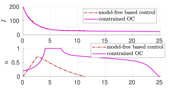
(a) Evolution of the infected state $I$ versus time (in years).

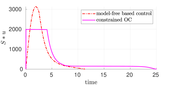
(b) Evolution of the controlled medication $u$ versus time (in years).

Figure 2: Evaluation of the unconstrained model-free based control with slope as first sequence.

(a) Evolution of the infected state $I$ versus time (in years).

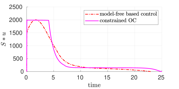
(b) Evolution of the controlled medication $u$ versus time (in years).

Figure 3: Evaluation of the constrained model-free based control: slope as first sequence including the constraint (3.1) – case I.

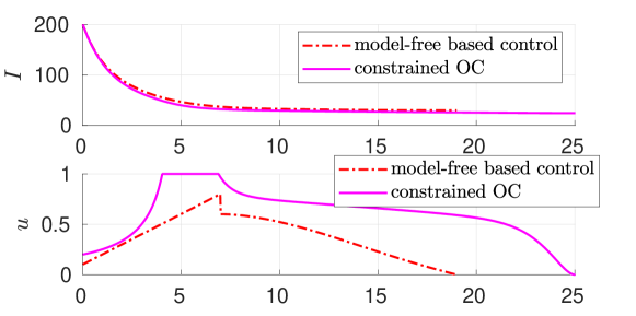
(a) Evolution of the infected state $I$ versus time (in years).

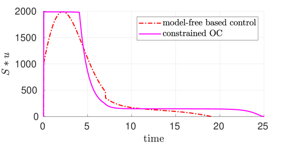
(b) Evolution of the controlled medication $u$ versus time (in years).

Figure 4: Evaluation of the constrained model-free based control: slope as first sequence including the constraint (3.1) – case II.

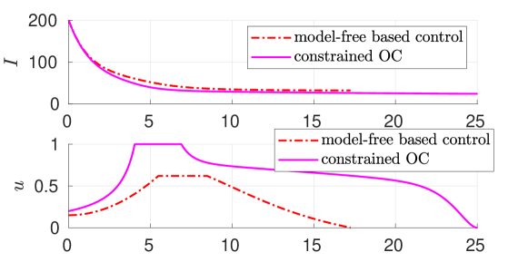
(a) Evolution of the infected state $I$ versus time (in years).

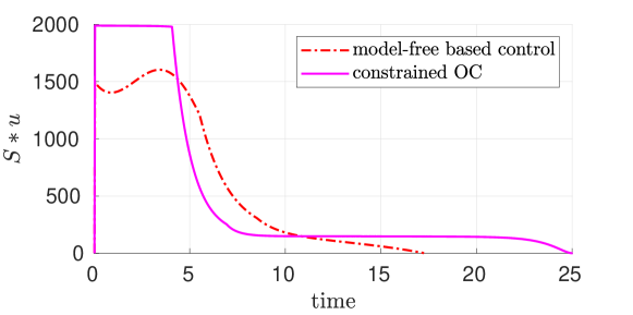
(b) Evolution of the controlled medication $u$ versus time (in years).

Figure 5: Evaluation of the constrained model-free based control: quadratic as first sequence including the constraint (3.1) – case I.

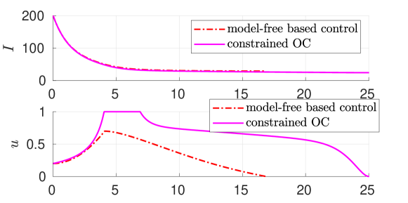
(a) Evolution of the infected state $I$ versus time (in years).

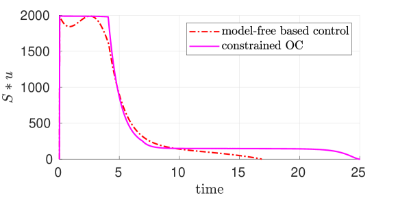
(b) Evolution of the controlled medication $u$ versus time (in years).

Figure 6: Evaluation of the constrained model-free based control: quadratic as first sequence including the constraint (3.1) – case II.

From Figure 2a, we see that although the model-free based control and the classical optimal control approaches propose completely different control functions, the associated number of HIV infected individuals $I(t)$, $t\in[0,25]$, are very similar. Interestingly, the control solution of the model-free based control is active in a much smaller interval of time that the one obtained with the classical optimal control approach: $T_{e}=11.3$ versus $T_{e}=25$ (see first line of Table 1). Analogous conclusions are taken from Figures 3a–6a.

It should be noted, however, that in Figure 2b the control obtained from the model-free based approach does not satisfy the mixed state-control constraint $S(t)u(t)\leq 2000$ for all $t$. In order to satisfy this constraint one must increase the time interval where the model-free control is active, see Figures 3b–6b. This depends on the configuration of the initial transient of the control (slope or quadratic), see Figures 3a–6a and Table 1.

4 Discussion

The proposed control sequence can be considered as “quasi-optimal” in the sense that it does not obey to the Pontryagin maximum principle, so it is not an optimal control by definition, but it offers similar properties in terms of cost criteria minimization and reduction of the duration of treatment that is assured by our procedure.

The sequence is fully parametrized thanks to the initial transient coefficients $(L$ or $Q)$ associated to $u_{max}$, including the $\mathcal{C}_{\pi}$-parameters for the decreasing transient, that must be adjusted according to the evolution of the infected state. In particular, the maximum value on the product $Su$ depends on the “speed” of the increasing transient as well as the final value $I(T_{e})$, which depends on the “speed” of the increasing transient, the initial value $u_{0}$, and the feedback control that stabilizes $I$ through the decreasing transient. The transient slope plays a key role in the “accuracy” of the initial decrease of the infected state since a sufficient dose of the medication $u$ must be injected to the population in order to maintain the infected state to a lower level. Therefore, the maximum value of $u$ is a trade-off between the constraint $Su\leq\gamma_{max}$ to be satisfied and the duration of the treatment. Figure 2 illustrates a rather quick treatment, involving thus a fast initial transient but the constraint $Su\leq 2000$ is not satisfied; slower medical treatment for which the injection of the medication $u$ takes more time due to the constraint $Su\leq 2000$, can reduce the final asymptotic value $I(T_{e})$ despite not necessarily fully reducing the cost criteria. The model-free based control aims to relax the treatment until $u=0$ is reached. A first tuning has been made according to the gained experience and a more precise tuning can be performed using [19]. The numerical evaluation of the cost criteria shows that our approach is globally better in terms of energy minimization. Moreover, the time-pondered criteria shows that the proposed control procedure is favorable to our approach taking into account the reduction of the duration of the treatment. These results illustrate afterwards that tuning the parameters of the proposed control sequence is a trade-off between considering minimizing the cost criteria, or minimizing the final value $I(T_{e})$, depending of additional constraints.

We remark that the model-free based control could have been also used to drive the initial transient instead of the slope or the quadratic function, but the current algorithm offers slower performances at the very beginning to initiate the increase of the medication that prevents it to deal with, for example, the constraint $Su\leq 2000$.

5 Conclusion and future work

We have considered a SICAE epidemiological model for HIV/AIDS transmission, proposing, for the first time in the literature, a model-free based approach to minimize the number of infected individuals. This approach consists in initializing PrEP medication, using a basic linear or quadratic function, and after that creating a direct feedback to control the decrease of infected individuals with respect to the considered measure of infected cases. Globally, the advantages of the proposed approach, when compared with the classical optimal control based on the Pontryagin Maximum Principle, is that it does not need any a priori knowledge of the model and a simple tuning of the proposed control sequence values allows good performances in terms of “energy” minimization as well as minimization of the medical treatment duration. We concluded that our control strategy highlights interesting performances compared with the classical optimal control approach used in [23].

From a biological point of view, our application of the model-free based control approach allows to propose new solutions for the implementation of PrEP in the prevention of HIV transmission, considering the constraints associated to the limitations on the availability of medicines for HIV and on number of individuals that the health systems have capacity to follow up during their treatment. To the best of our knowledge, we were the first to apply the model-free based control approach in the context of epidemiology.

Future work may include replacing the slope or the quadratic initial transient by an optimal control; improvement of the proposed model-free based control; implementation and comparison with the original Fliess–Join version of the model-free control, as it has been done, for example, for the glycemia control [11]. Stability issues regarding the closed loop are very important and a promising LMI framework dedicated to study the stability of optimization algorithms is also of interest [7, 20].

References

- [1] (MR3157723) [10.1016/j.automatica.2013.10.012] K. J. Aström, P. R. Kumar, Control: A perspective, Automatica, 50 1 (2014), 3–43.
- [2] [10.1109/ECC.2016.7810602] O. Bara, M. Fliess, C. Join, J. Day, S. Djouadi, Model-free immune therapy: A control approach to acute inflammation, 15th European Control Conference (ECC’16), (2016).
- [3] (MR3789959) [10.1016/j.jtbi.2018.04.003] O. Bara, M. Fliess, C. Join, J. Day, S. M. Djouadi, Toward a model-free feedback control synthesis for treating acute inflammation, Journal of Theoretical Biology, 448 (2018), 26–37.
- [4] CDC, Pre-Exposure Prophylaxis (PrEP), Division of HIV/AIDS Prevention, National Center for HIV/AIDS, Viral Hepatitis, STD, and TB Prevention, Centers for Disease Control and Prevention, https://www.cdc.gov/hiv/risk/prep/index.html, Page last reviewed: August 6, 2021.
- [5] [10.1016/S0140-6736(13)61809-7] S. G. Deeks, S. R. Lewin, D. V. Havlir, The end of AIDS: HIV infection as a chronic disease, The Lancet, 382 9903 (2013), 1525–1533.
- [6] (MR3808514) [10.1016/j.aml.2018.05.005] J. Djordjevic, C. J. Silva, D. F. M. Torres, A stochastic SICA epidemic model for HIV transmission, Appl. Math. Lett. 84 (2018), 168–175. arXiv:1805.01425
- [7] (MR3856216) [10.1137/17M1136845] M. Fazlyab, A. Ribeiro, M. Morari, V.M. Preciado, Analysis of Optimization Algorithms via Integral Quadratic Constraints: Nonstrongly Convex Problems, SIAM Journal on Optimization, 28 3 (2018), 2654–2689.
- [8] M. Fliess, C. Join, Commande sans modèle et commande à modèle restreint, e-STA Sciences et Technologies de l’Automatique, SEE - Société de l’Electricité, de l’Electronique et des Technologies de l’Information et de la Communication, 5(4) (2008), 1–23.
- [9] [10.3182/20090706-3-FR-2004.00256] M. Fliess, C. Join, Model-free control and intelligent PID controllers: Towards a possible trivialization of nonlinear control?, IFAC Proceedings Volumes, 42(10) (2009), 1531–1550.
- [10] (MR3172473) [10.1080/00207179.2013.810345] M. Fliess, C. Join, Model-free control, International Journal of Control, 86 12 (2013), 2228–2252.
- [11] [10.1002/rnc.5657] M. Fliess, C. Join, An alternative to PIs and PIDs: Intelligent proportional-derivative regulators, International Journal of Robust and Nonlinear Control, in press. DOI: 10.1002/rnc.5657
- [12] [10.1109/CoDIT.2019.8820297] K. Hamiche, M. Fliess, C. Join, H. Abouaïssa, Bullwhip effect attenuation in supply chain management via control-theoretic tools and short-term forecasts: A preliminary study with an application to perishable inventories, 6th International Conference on Control, Decision and Information Technologies (CoDIT), 2019, 1492–1497.
- [13] [10.1016/j.ifacol.2017.08.1167] C. Join, J. Bernier, S. Mottelet, M. Fliess, S. Rechdaoui-Guérin, S. Azimi, V. Rocher, A simple and efficient feedback control strategy for wastewater denitrification, IFAC-PapersOnLine 50 (2017), no. 1, 7657–7662.
- [14] (MR3999700) [10.19139/soic.v7i3.834] E. M. Lotfi, M. Mahrouf, M. Maziane, C. J. Silva, D. F. M. Torres and N. Yousfi, A minimal HIV-AIDS infection model with general incidence rate and application to Morocco data, Stat. Optim. Inf. Comput. 7 (2019), no. 2, 588–603. arXiv:1812.06965
- [15] L. Michel, A para-model agent for dynamical systems, preprint arXiv:1202.4707, (2018).
- [16] [10.1109/TBME.2017.2698036] T. MohammadRidha, M. Aït-Ahmed, L. Chaillous, M. Krempf, I. Guilhem, J.-Y. Poirier, C. H. Moog, Model Free iPID Control for Glycemia Regulation of Type-1 Diabetes, IEEE Transactions on Biomedical Engineering, 65 1 (2018), 199–206.
- [17] [10.1137/1.9781611974072.9] T. MohammadRidha, C. Moog, E. Delaleau, M. Fliess, C. Join, A variable reference trajectory for model-free glycemia regulation, SIAM Conference on Control its Applications (SIAM CT15), (2015).
- [18] [10.1016/j.arcontrol.2019.08.004] T. P. Nascimento, M. Saska, Position and attitude control of multi-rotor aerial vehicles: A survey, Annual Reviews in Control, 48 (2019), 129–146.
- [19] [10.1145/3085592] M. Porcelli, P.L. Toint, BFO, A Trainable Derivative-Free Brute Force Optimizer for Nonlinear Bound-Constrained Optimization and Equilibrium Computations with Continuous and Discrete Variables, ACM Transactions on Mathematical Software, 44 1, no. 6 (2017), 1–25.
- [20] (MR4267491) [10.1137/20M1364138] J. M. Sanz-Serna, K. C. Zygalakis, The connections between Lyapunov functions for some optimization algorithms and differential equations, SIAM J. Numer. Anal., 59 (3) (2021), 1542–1565.
- [21] (MR3392642) [10.3934/dcds.2015.35.4639] C. J. Silva, D. F. M. Torres, A TB-HIV/AIDS coinfection model and optimal control treatment, Discrete Contin. Dyn. Syst., 35 no. 9 (2015), 4639–4663. arXiv:1501.03322
- [22] [10.1016/j.ecocom.2016.12.001] C. J. Silva, D. F. M. Torres, A SICA compartmental model in epidemiology with application to HIV/AIDS in Cape Verde, Ecological Complexity, 30 (2017), 70–75. arXiv:1612.00732
- [23] (MR3714435) [10.3934/dcdss.2018008] C. J. Silva, D. F. M. Torres, Modeling and optimal control of HIV/AIDS prevention through PrEP, Discrete Contin. Dyn. Syst. Ser. S, 11 no. 1 (2018), 119–141. arXiv:1703.06446
- [24] (MR3980195) [10.1016/j.matcom.2019.03.016] C. J. Silva and D. F. M. Torres, Stability of a fractional HIV/AIDS model, Math. Comput. Simul. 164 (2019), 180–190. arXiv:1903.02534
- [25] (4175342) [10.1007/978-3-030-49896-2_6] C. J. Silva and D. F. M. Torres, On SICA models for HIV transmission. In: Mathematical Modelling and Analysis of Infectious Diseases, Studies in Systems, Decision and Control 302 (2020), 155–179. arXiv:2004.11903
- [26] S. Tebbani, M. Titica, C. Join, M. Fliess, D. Dumur, Model-based versus model-free control designs for improving microalgae growth in a closed photobioreactor: Some preliminary comparaisons, The 24th Mediterranean Conference on Control and Automation (MED’16), IEEE (2016), 683–688.
- [27] (MR4276109) [10.3934/mbe.2021231] S. Vaz and D. F. M. Torres, A dynamically-consistent nonstandard finite difference scheme for the SICA model, Math. Biosci. Eng. 18 (2021), no. 4, 4552–4571. arXiv:2105.10826
- [28] (MR4261252) [10.1186/s13662-021-03392-y] X. Wang, C. Wang and K. Wang, Extinction and persistence of a stochastic SICA epidemic model with standard incidence rate for HIV transmission, Adv. Difference Equ. 2021, Paper No. 260, 17 pp.
- [29] [10.1016/S0140-6736(08)61115-0] D. P. Wilson, M. G. Law, A. E. Grulich, D. A. Cooper, J. M. Kaldor, Relation between HIV viral load and infectiousness: A model-based analysis, The Lancet, 372 no. 9635 (2008), 314–320.
- [30] (MR4279814) [10.1002/mma.7292] M. Zaka Ullah and D. Baleanu, A new fractional SICA model and numerical method for the transmission of HIV/AIDS, Math. Methods Appl. Sci. 44 (2021), no. 11, 8648–8659.