Rise and fall of plaquette order in Shastry-Sutherland magnet revealed by pseudo-fermion functional renormalization group

Abstract

The Shastry-Sutherland model as a canonical example of frustrated magnetism has been extensively studied. The conventional wisdom has been that the transition from the plaquette valence bond order to the Neel order is direct and potentially realizes a deconfined quantum critical point beyond the Ginzburg-Landau paradigm. This scenario however was challenged recently by improved numerics from density matrix renormalization group which offers evidence for a narrow gapless spin liquid between the two phases. Prompted by this controversy and to shed light on this intricate parameter regime from a fresh perspective, we report high-resolution functional renormalization group analysis of the generalized Shastry-Sutherland model. The flows of over 50 million running couplings provide a detailed picture for the evolution of spin correlations as the frequency/energy scale is dialed from the ultraviolet to the infrared to yield the zero temperature phase diagram. The singlet dimer phase emerges as a fixed point, the Neel order is characterized by divergence in the vertex function, while the transition into and out of the plaquette order is accompanied by pronounced peaks in the plaquette susceptibility. The plaquette order is suppressed before the onset of the Neel order, lending evidence for a finite spin liquid region for $J_{1}/J_{2}\in(0.77,0.82)$, where the flow is continuous without any indication of divergence.

Forty years after the introduction of the Shastry-Sutherland (SS) model Sriram Shastry and Sutherland (1981), its ground state phase diagram remains inconclusive. The model describes quantum spins on the square lattice with competing antiferromagnetic exchange interactions, $J_{1}$ for the horizontal/vertical bonds and $J_{2}$ for the decimated diagonal bonds connecting the empty plaquettes, see Fig. 1. Owing to the frustration, the model has long been suspected to host exotic ground states and phase transitions. A large body of theoretical works have established the existence of three phases, see e.g. Miyahara and Ueda (2003) and Lee et al. (2019); Yang et al. (2021) for a synopsis of earlier and recent results, respectively. The $J_{1}<J_{2}/2$ limit is exactly solvable and the ground state is a product state of diagonal dimers (spin singlets). For intermediate value of $J_{1}/J_{2}$, the ground state is a plaquette valence bond solid, while Neel order takes over for large $J_{1}/J_{2}$. The most interesting, and controversial, question regards the nature of the plaquette-to-Neel (pN) transition: is it conventional, a deconfined quantum critical point, or through an additional spin liquid phase?

Remarkably, the SS model has an almost ideal realization in $\mathrm{SrCu_{2}(BO_{3})_{2}}$ crystals, where phase transitions can be induced by tuning the hydrostatic pressure Kageyama et al. (1999); Miyahara and Ueda (1999). Inelastic neutron scattering found signatures of the plaquette phase Zayed et al. (2017), and heat capacity measurements confirmed the dimer-to-plaquette transition Guo et al. (2020); Jiménez et al. (2021). Yet a direct plaquette-to-Neel transition was not observed in the anticipated pressure range. These experiments renewed the effort to examine this intriguing region using the state-of-the-art numerical techniques. Earlier tensor network (iPEPS) calculations confirmed the plaquette phase within the region $J_{1}/J_{2}\in[0.675,0.765]$ Koga and Kawakami (2000); Corboz and Mila (2013); Boos et al. (2019); Wietek et al. (2019); Shi et al. (2021) and a weak first order pN transition. A recent density matrix renormalization group (DMRG) study Lee et al. (2019) with cylinders of circumference up to ten sites yielded similar phase boundary $J_{1}/J_{2}\in[0.675,0.77]$ but a continuous pN transition with spin correlations supporting a deconfined quantum critical point. Another DMRG using cylinder circumference up to 14 sites concludes that a spin liquid phase exists in the window $J_{1}/J_{2}\in[0.79,0.82]$ between the plaquette and the Neel phase Yang et al. (2021). A core difficulty in reaching a consensus is attributed to the near degeneracy of the competing orders in this region. The finite-size limitation of DMRG means that the ground state can only be inferred by extrapolation via careful finite size scaling analysis.

The size restriction prompts us to adopt an alternative approach diametrically opposed to exact diagonalization or DMRG on finite systems. The algorithm directly accesses the infrared and thermodynamic limit while treating all competing orders on equal footing without bias. It starts from the microscopic spin Hamiltonian and successively integrates out the higher frequency fluctuations with full spatial (or equivalently momentum) resolution retained at each step. The scale-dependent effective couplings and correlation functions are obtained by numerically solving the Functional Renormalization Group (FRG) flow equations Polchinski (1984); Wetterich (1993); Morris (1994). As the frequency scale $\Lambda$ slides from $J_{1,2}$ down to zero, the zero temperature phase diagram is determined. Such FRG approach to quantum spin systems, first established in 2010 Reuther and Wölfle (2010), has yielded insights for many frustrated spin models. But its application to the SS model has not been successful, perhaps due to two reasons. First, in contrast to the Neel order, the dimer or the plaquette order cannot be inferred naively from the divergence of vertex functions, making it challenging to locate their phase boundaries. Second, as we shall show below, the pN transition region is better understood by examining a generalized model that reduces to the SS model in a particular limit.

In this work, high resolution FRG analysis of the generalized SS model is achieved by overcoming these technical barriers. To maintain sufficient momentum and frequency resolution, one must keep track of millions of running couplings at each FRG step. The calculation is made possible by migrating to the GPU platform which led to performance improvement by orders of magnitude Keles and Zhao (2018a, b). Despite being a completely different approach, the phase boundaries predicted from our FRG are remarkably close to the state-of-the-art DMRG. The agreement further establishes FRG as an accurate technique for frustrated quantum magnetism. Most importantly, the plaquette susceptibility from FRG indicates the plaquette order terminates around $J_{1}/J_{2}\approx 0.77$ before the onset of weak Neel order around $J_{1}/J_{2}\approx 0.82$. It supports the existence of a spin liquid region between the plaquette and Neel phase proposed in Ref. Yang et al. (2021). Thus, the SS model is a strong candidate to host spin liquid, and $\mathrm{SrCu_{2}(BO_{3})_{2}}$ offers exciting opportunity to realize and probe the elusive spin liquid phase.

Model and pseudofermion FRG.— Our starting point is the generalized Shastry-Sutherland Hamiltonian Läuchli et al. (2002)

$$H=\kappa J_{1}\sum_{\langle i,j\rangle^{\prime}}\mathbf{S}_{i}\cdot\mathbf{S}_{j}+J_{1}\sum_{\langle i,j\rangle^{\prime\prime}}\mathbf{S}_{i}\cdot\mathbf{S}_{j}+J_{2}\sum_{i,j\in\text{diag}}\mathbf{S}_{i}\cdot\mathbf{S}_{j}$$ (1)

where $\mathbf{S}_{i}$ are spin one-half operators ($S=1/2$), $i,j$ label the sites, and $J_{1,2}>0$ are antiferromagnetic exchange couplings. The first (second) sum is over nearest neighbors on the square lattice represented by the solid (dashed) black lines in Fig. 1(a), the last sum is over the alternating diagonal bonds indicated by the red lines. The original SS model corresponds to the limit $\kappa=1$ Sriram Shastry and Sutherland (1981); Miyahara and Ueda (2003). A small $\delta J_{1}=(\kappa-1)J_{1}$ acts as a source field to break the double degeneracy and favor valence bond order within the shaded plaquettes. It plays a crucial role in our analysis and facilitates the calculation of plaquette susceptibility. We will stay close to the limit $\kappa\rightarrow 1$ throughout.

To predict the phase diagram of Hamiltonian Eq. (1), FRG finds its generating functional, i.e. an effective field theory parametrized by self-energies, four-point and higher-order vertices, for each given frequency/energy scale $\Lambda$. The self-energies and vertices obey the formally exact flow equations that can be truncated and solved numerically. More specifically, the many-spin problem is first converted to an interacting fermion problem using the pseudofermion representation Reuther and Wölfle (2010), $S_{i}^{\mu}=(1/2)\sigma^{\mu}_{\alpha\beta}\psi^{\dagger}_{i\alpha}\psi_{i\beta}$. Here $\sigma^{\mu}$ are the Pauli matrices, and $\psi_{i\beta}$ annihilates a fermion at site $i$ with spin $\beta=\uparrow,\downarrow$ etc.. The resultant fermion Hamiltonian only has quartic interactions but no kinetic energy term (the fermions are localized and constrained at one particle per site). So the bare single-particle Green function $G_{0}(\omega)=1/i\omega$ with $\omega$ being the frequency Reuther and Wölfle (2010). Then the flow equations for the interacting fermion problem can be solved by generalizing the expansion and truncation schemes extensively benchmarked for strongly correlated electronic materials Metzner et al. (2012); Kopietz et al. (2010).

The implementation of psuedofermion FRG are well documented in the original work Reuther and Wölfle (2010) and later improvements Buessen and Trebst (2016); Iqbal et al. (2016a, b); Hering and Reuther (2017); Baez and Reuther (2017); Buessen et al. (2018a, b); Hering et al. (2019); Buessen et al. (2019); Iqbal et al. (2019); Buessen and Kim (2021); Niggemann et al. (2021); Kiese et al. (2021); Hering et al. (2021). A brief outline is as follows. Starting from an ultraviolet scale $\Lambda=\Lambda_{UV}\gg J_{1,2}$ and using the bare interaction in Eq. (1) and bare Green function to set up the initial condition, the coupled integro-differential equations for the scale-dependent self-energy $\Sigma^{\Lambda}(\omega)$ and four-point vertex $\Gamma^{\Lambda}_{i_{1}i_{2}}(\omega_{1}^{\prime},\omega_{2}^{\prime};\omega_{1},\omega_{2})$ are solved successively in small steps along a discretized grid of the frequency/energy scale $\Lambda$ until it is reduced down to the infrared $\Lambda=\Lambda_{IR}\rightarrow 0$. During the flow, the self-energy $\Sigma^{\Lambda}(\omega)$ is renormalized to gain nontrivial frequency dependence as higher frequency fluctuations induce retarded interactions. But it remains site-independent, i.e. fermions hopping is prohibited. The four-point vertices $\Gamma^{\Lambda}$ (effective interactions) carry multiple indices: $i_{1}$ and $i_{2}$ for lattice sites whereas $\omega_{1}^{\prime},\omega_{2}^{\prime}$ and $\omega_{1},\omega_{2}$ are frequencies for the pair of sites before and after the interaction. Contributions from higher order vertices are approximated by the Katanin term Katanin (2004).

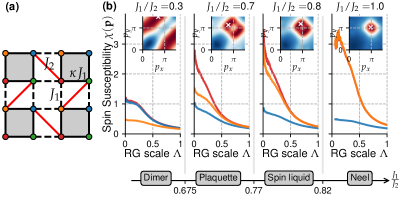
Figure 1: Generalized Shastry-Sutherland model and its zero temperature phase diagram from FRG. (a) The competing exchange couplings in model Eq. (1) include $\kappa J_{1}$ and $J_{1}$ for the black solid and dashed bonds respectively, and $J_{2}$ for the red bonds. The four sites within the unit cell (shaded square) are labelled by color red, green, blue and yellow respectively. (b) The phase diagram for $\kappa=1$ consists of four phases separated by three critical points as $J_{1}/J_{2}$ is varied. A representative point is chosen for each phase to illustrate the typical RG flows of the spin susceptibilities $\chi(\mathbf{p})$ in leading channels (i.e. different values of $\mathbf{p}$, see main text). The corresponding insets show the profile of $\tilde{\chi}_{r}(\mathbf{p})$ in the infrared limit $\Lambda\rightarrow 0$. The white $\times$ indicates its peak position in the momentum space $(p_{x},p_{y})$.

Care must be exercised to efficiently parametrize the vertices in order to render the numerical task tractable. In particular, the SS model has non-symmorphic lattice symmetry, with four sites per unit cell shown in colors $\alpha=r,g,b,y$ in Fig. 1 and no $C_{4}$ symmetry as in the $J_{1}$-$J_{2}$ model. To avoid using color indices in $\Gamma^{\Lambda}_{i_{1}i_{2}}$, we pick a $\alpha=r$ site located at the origin as $i_{1}$. Other vertices for sites of different color $\alpha=g,b,y$ can be obtained from the central $r$-site with appropriate rotation and lattice translation sup . We retain all $i_{2}$ within a radius $|\mathbf{r}_{i_{1}}-\mathbf{r}_{i_{2}}|<R_{\mathrm{max}}$ in $\Gamma^{\Lambda}_{i_{1}i_{2}}$ and emphasize that the FRG equations describe infinite systems without a boundary. Here $R_{max}$ merely places an upper cutoff for the correlations retained in the numerics. As to the frequency variables, we rewrite $\Gamma^{\Lambda}(\omega_{1}^{\prime},\omega_{2}^{\prime};\omega_{1},\omega_{2})$ as functions of the Mandelstam variables $s$, $t$ and $u$ Reuther and Wölfle (2010) which manifestly enforce the frequency conservation. Finally, we discretize the frequency using a logarithmic mesh of $N_{\omega}$ points extending from the ultraviolet scale $\Lambda_{UV}=10^{2}J_{2}$ to the infrared scale $\Lambda_{IR}=10^{-2}J_{2}$. Typically, $N_{\omega}=48$ provides good frequency resolution, and further increasing $N_{\omega}$ will not alter the results appreciably. We take $R_{max}=10$ which amounts to $N_{L}=441$ lattice sites within the correlation radius. In total, this gives a coupled system of $N_{L}\times N_{\omega}^{3}\sim$ 50 million running couplings.

Correlation functions and susceptibilities.— To detect the emergence of long range order as $\Lambda\rightarrow 0$, correlation functions at each renormalization scale can be obtained from the $\Sigma^{\Lambda}$ and $\Gamma^{\Lambda}$ via standard calculations involving Feynman diagrams. For example, the spin-spin correlation function is given by

$$\chi_{ij}(\omega) = \int_{0}^{\infty}d\tau e^{i\omega\tau}\langle TS_{i}^{z}(\tau)S_{j}^{z}(0)\rangle$$ (2)

$$= \leavevmode\hbox to166.16pt{\vbox to27.28pt{\text{[drawing]}}}, S_{i}^{z} S_{j}^{z} S_{j}^{z} S_{j}^{z} + S_{i}^{z} S_{j}^{z} S_{j}^{z} S_{j}^{z} +$$

where black dots represent the spin matrix $S_{i}^{z}=\sigma^{z}/2$, filled square represents vertex $\Gamma^{\Lambda}$ and lines with arrows are dressed Green functions that contain the self-energy. The scale dependence of $\chi$ is suppressed for brevity. We find that it is necessary to distinguish the flows of spin correlations for different bonds, i.e. pairs of $(i,j)$, because the symmetry breaking patterns in the SS model are rather complex and involving valence bond orders. For a given site $i$ of color $\alpha$, one can find $\tilde{\chi}_{\alpha}(\mathbf{p})$, the Fourier transform of Eq. (2) in the limit of $\omega\rightarrow 0$. It is also convenient to define spin susceptibility

$$\chi(\mathbf{p})=\lim_{\omega\rightarrow 0}\frac{1}{4}\sum_{\alpha}\sum_{j}e^{i\mathbf{p}\cdot(\mathbf{r}_{\alpha}-\mathbf{r}_{j})}\chi_{ij}(\omega)=\frac{1}{4}\sum_{\alpha}\tilde{\chi}_{\alpha}(\mathbf{p}),$$ (3)

where the $\alpha$ sum is over the four sites of different colors within the unit cell, the $j$ sum is over all sites, and the limit $\omega\rightarrow 0$ is taken in the end. The spin susceptibility defined in Eq. (3) has no bond resolution, but its divergence (or lack thereof) and its profile in momentum space offer a quick diagnosis of the incipient orders as the ratio $J_{1}/J_{2}$ is changed. Finally, we define a set of plaquette susceptibilities to detect the plaquette valence bond order. They measure the bond-resolved responses, e.g. the change in $\chi_{ij}$, due to a small bond modulation

$${\chi}^{P}_{ij}\equiv\left.-\frac{1}{J_{1}}\frac{\partial\chi_{ij}}{\partial\kappa}\right|_{\kappa\rightarrow 1}=\left.-\frac{\partial\chi_{ij}}{\partial(\delta J_{1})}\right|_{\delta J_{1}\rightarrow 0}$$ (4)

with $J_{1}$ and $J_{2}$ fixed. A dramatic enhancement of the $\chi_{ij}^{P}$ around the shaded plaquettes indicates an instability against a small fluctuation of modulation $\delta J_{1}$. To compute ${\chi}_{ij}^{P}$, we perform two runs of FRG flow with bare couplings $(\kappa J_{1}=J_{1}+\delta J_{1},J_{1},J_{2})$ and $(J_{1},J_{1},J_{2})$ for a given bond $(i,j)$. The procedure is expensive but provides invaluable insights.

Phase diagram.— The final results of our FRG calculation are summarized in the phase diagram shown in Fig. 1(b). It contains four phases as $J_{1}/J_{2}$ is varied at fixed $\kappa=1$. For each phase, a representative value of $J_{1}/J_{2}$ is chosen to illustrate its characteristic FRG flow pattern in two complementary ways. First is the momentum distribution $\tilde{\chi}_{r}(\mathbf{p})$ near the end of the flow (insets), where the peak momenta are labelled by white ‘$\times$’ in the extended Brillouin zone . Next is the flow of spin susceptibility ${\chi}(\mathbf{p})$ with the RG scale $\Lambda$ (main panels) for different channels, i.e., different values of $\mathbf{p}$. For example, the channel $\mathbf{p}=(\pi,0)$ is shown in blue, the $(\pi,\pi)$ channel in orange, while the flow for the peak momenta labelled by ‘$\times$’ is in red. Clearly, the leading channels for the four phases are distinct. Take the case $J_{1}/J_{2}=1.0$ for example, from the inset it is clear that $\tilde{\chi}_{r}(\mathbf{p})$ is peaked at $\mathbf{p}=(\pi,\pi)$. Accordingly, the FRG flow for ${\chi}(\pi,\pi)$ (in orange) is most dominant and rises rapidly as $\Lambda$ is reduced. The flow breaks down around $\Lambda^{*}\approx 0.2$, signaling a physical divergence and the onset of magnetic long-range order as seen in many FRG calculations. Thus the Neel phase can be identified unambiguously from the $(\pi,\pi)$ peak and the flow divergence.

Outside the Neel phase, the flows appear smooth down to the lowest $\Lambda$. This is perhaps not that surprising because spin rotational symmetry is not broken in the dimer or plaquette phase. Yet by inspecting the two cases $J_{1}/J_{2}=0.3$ and $0.7$ in Fig. 1, it is apparent that their spin correlations are rather different, e.g., they have different peak momenta or leading channels. Unfortunately, the information contained in $\chi(\mathbf{p})$ or $\tilde{\chi}_{\alpha}(\mathbf{p})$ is too crude to differentiate the dimer from the plaquette phase. In what follows, we show that this can be achieved by the FRG flow of bond-resolved spin correlation $\chi_{ij}$.

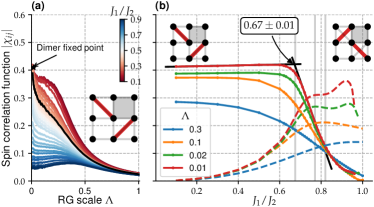
Figure 2: The dimer and spin liquid phase as the fixed points of the flow of spin-spin correlation functions $\chi_{ij}(\omega\rightarrow 0)$. (a) Flows of $\chi_{ij}$ for the dimer bonds (red lines in inset) converge to a constant $\approx 0.41$ in the infrared limit for all $J_{1}/J_{2}$ values (color coded, see the colorbar) up until 0.67 indicated by the solid black line. (b) The scale-dependent $\chi_{ij}$ (solid lines) for the dimer bonds becomes flat against $J_{1}/J_{2}$ in the infrared limit. Linear regression (black lines) gives the dimer to plaquette transition point $(J_{1}/J_{2})_{c}=0.67$. The dashed lines represent $\chi_{ij}$ for another set of diagonal bonds (inset at the upper right corner) orthogonal to the dimer bonds. As $\Lambda\rightarrow 0$, it becomes flat for $J_{1}/J_{2}$ between 0.77 and 0.82 where spin liquid is postulated to exist.

Dimer phase as a fixed point.—Fig. 2(a) compares the flows of $\chi_{ij}$ for the diagonal bond (red lines in the inset) at different values of $J_{1}/J_{2}$. One notices a remarkable phenomenon: for all $J_{1}/J_{2}<0.6$, they flow to the same exact value $\approx 0.41$ in the infrared $\Lambda\rightarrow 0$. This renormalization group fixed point defines a robust phase with constant spin correlation along the diagonal. This is nothing but the dimer phase, in accordance with the known fact that the ground state wave function in this region is a product state of isolated spin singlets, frozen with respect to $J_{1}/J_{2}$ with constant energy up to a critical point. To determine its phase boundary, Fig. 2(b) plots the diagonal bond correlation in the infrared limit versus $J_{1}/J_{2}$. It stays completely flat before dropping rapidly in a linear fashion. Linear regression (black lines) yields an intersection point at $J_{1}/J_{2}=0.67$ which we take as the estimated phase transition point. This critical value is impressively close to 0.675 from large-scale DMRG Lee et al. (2019). The agreement provides strong evidence for the validity and accuracy of our FRG calculation.

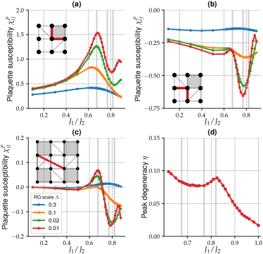
Figure 3: Identification of the phase boundaries from bond-resolved plaquette susceptibility $\chi^{P}_{ij}$, which measures the response of a given bond $(i,j)$ [red lines in insets] to a small increase $\delta J_{1}$ in the shaded squares. (a) A pronounced peak of $\chi^{P}_{\blacksquare}$ around $J_{1}/J_{2}=0.67$ signals the onset of plaquette order. (b) The suppression dip of $\chi^{P}_{\square}$ at $0.77$ indicates the plaquette order is superseded by a new phase, the spin liquid with distinct inter-plaquette correlations. (c) An example of longer range $\chi^{P}_{ij}$ that also develops peak/dip at the two critical points above. (d) The momentum space degeneracy $\eta$ of $\tilde{\chi}_{r}(\mathbf{p})$ is peaked at $J_{1}/J_{2}\approx 0.82$, which marks the transition into the Neel phase.

Plaquette valence bond solid.—Identification of plaquette order from FRG has been an open challenge. In earlier studies, a plaquette susceptibility $\chi_{PVB}$ was defined as the propensity towards translational symmetry breaking with respect to a small bond modulation bias Reuther and Wölfle (2010); Iqbal et al. (2016a, 2019). Enhancement of $\chi_{PVB}$ has been reported, but to our best knowledge, plaquette order has not been positively identified using pseudofermion FRG so far. For the generalized SS model, we have confirmed that $\chi_{PVB}$ is indeed enhanced within a broad region stretching from $J_{1}/J_{2}\sim 0.5$ to $0.7$ when compared to its values within the Neel phase (see sup for details). But it only exhibits a smooth crossover with $J_{1}/J_{2}$ due to the lack of bond resolution. This has motivated us to introduce a more refined measure, the bond-resolved plaquette susceptibility ${\chi}^{P}_{ij}$ in Eq. (4).

Fig. 3(a) illustrates the ${\chi}^{P}_{ij}$ for the horizontal/vertical bonds within the slightly strengthened plaquettes (shaded squares), denoted by $\chi^{P}_{\blacksquare}$. While it is more or less featureless at the ultraviolet scale, as RG steps are taken and $\Lambda$ is reduced, $\chi^{P}_{\blacksquare}$ gains nontrivial dependence on $J_{1}/J_{2}$. In particular, in the infrared limit ${\chi}^{P}_{\blacksquare}$ develops a pronounced peak around $J_{1}/J_{2}\approx 0.67$ . The dramatic enhancement of plaquette susceptibility marks the onset of plaquette order. This independent diagnosis of the dimer-to-plaquette transition agrees very well with the linear regression result above, showing the self-consistency of our FRG and the advantage of introducing the quantity ${\chi}^{P}_{ij}$. It is not a divergence because higher-order vertices are truncated in the current implementation. The onset of plaquette order also manifests in longer range inter-plaquette correlations. Fig. 3(c) depicts the $\chi^{P}_{ij}$ for a bond between an $r$-site and a $b$-site from two shaded squares along the lattice diagonal. It too has an enhancement peak at $J_{1}/J_{2}\approx 0.67$.

Further analysis of ${\chi}^{P}_{ij}$ also points to the demise of the plaquette phase. A pristine plaquette order is adiabatically connected to the limit of decoupled plaquette singlets (shaded squares in Fig. 1 without red or dashed bonds). Upon increasing $J_{1}/J_{2}$, the plaquette order eventually yields to a state with homogeneous bond energies and very different spin correlations. One possibility is a liquid state where the shaded and empty squares are entangled to feature strong inter-plaquette correlations. The change in correlation is apparent in Fig. 3(c): after the peak, $\chi^{P}_{ij}$ changes sign to develop a sharp dip at $J_{1}/J_{2}\approx 0.78$, suggesting the onset of a new phase. This interpretation is supported by the plaquette susceptibility $\chi^{P}_{\square}$ shown in Fig. 3(b). It measures the change to the bonds around the empty plaquettes in response to $\delta J_{1}>0$ in the nearby shaded squares. When $J_{1}/J_{2}$ is reduced from above toward 0.77, a small $\delta J_{1}$ leads to significant weakening of the antiferromagnetic bonds (red lines) around the empty squares, i.e. decoupling of the shaded plaquettes to break translational symmetry. Thus the pronounce dip of $\chi^{P}_{\square}$ at $J_{1}/J_{2}\approx 0.77$ marks the upper critical point of the plaquette phase. At the very least, the dramatic variations of $\chi^{P}_{ij}$ are at odds with the scenario that the plaquette phase persists after $J_{1}/J_{2}\approx 0.77$.

A sliver of spin liquid.—The existence of a novel phase after $J_{1}/J_{2}\approx 0.77$ can be inferred independently from the spin correlation $\chi_{ij}$ for the diagonal bond shown in Fig. 2(b) (dashed lines). Here it becomes flat, i.e. independent of $J_{1}/J_{2}$, in the infrared limit. The behavior is distinct from that of a plaquette valence bond solid or a Neel antiferromagnet, for which $\chi_{ij}$ increases with $J_{1}$. Since the spin susceptibility flow is continuous down to $\Lambda\rightarrow 0$ as shown in Fig. 1(b), the only plausible scenario seems to be that this FRG fixed point corresponds to a liquid phase. With further increase in $J_{1}$, the flat top of diagonal $\chi_{ij}$ is terminated by an upturn around $J_{1}/J_{2}\sim 0.82$, signaling another phase transition. To precisely locate the onset of the Neel order, we adopt an independent criterion . In the postulated spin liquid region, the spin susceptibility $\tilde{\chi}_{r}(\mathbf{p})$ develops broad maxima, instead of a sharp peak, in momentum space, see the case of $J_{1}/J_{2}=0.8$ in Fig. 1(b). We can quantify the peak degeneracy by $\eta$, the percentage of $\mathbf{p}$ points with $\tilde{\chi}_{r}(\mathbf{p})\geq 0.9\mathrm{max}[\tilde{\chi}_{r}(\mathbf{p})]$. A similar method was employed in Nomura and Imada (2021) for a different system. The result is shown in Fig. 3(d). As the Neel phase is approached, the broad maxima coalesce into a sharp peak at $(\pi,\pi)$, after which $\eta$ drops quickly. The peak location of degeneracy $\eta$ at $J_{1}/J_{2}=0.82$ serves as an accurate estimation for the transition from the spin liquid to the Neel phase, in excellent agreement with the phase boundary obtained from large scale DMRG Yang et al. (2021).

Conclusions.—Our high-resolution FRG analysis of the SS model identifies four phases separated by three critical points summarized in Fig. 1. Key technical insights are retrieved by monitoring the renormalization group flows of bond-resolved spin-spin correlation functions and susceptibilities. The good agreement with other established numerical methods on the locations of the phase boundaries attests to the accuracy of FRG which takes into account quantum fluctuations in all the channels without bias by tracking millions of effective couplings at each scale $\Lambda$. The implementation and analysis strategies reported here can be applied to study other quantum spin Hamiltonians with unconventional magnetic orders using pseudofermion FRG. In particular, our result supports the existence of a finite spin liquid phase rather than a deconfined quantum critical point between the plaquette and Neel phase. It motivates future theoretical work to further elucidate the nature and extent of this phase, and precision measurements to locate and probe spin liquid in $\mathrm{SrCu_{2}(BO_{3})_{2}}$.