Estimates of $p$-harmonic functions in planar sectors

?abstractname?

Suppose that $p\in(1,\infty]$, $\nu\in[1/2,\infty)$, $\mathcal{S}_{\nu}=\left\{(x_{1},x_{2})\in\mathbb{R}^{2}\setminus\{(0,0)\}:|\phi|<\frac{\pi}{2\nu}\right\}$, where $\phi$ is the polar angle of $(x_{1},x_{2})$. Let $R>0$ and $\omega_{p}(x)$ be the $p$-harmonic measure of $\partial B(0,R)\cap\mathcal{S}_{\nu}$ at $x$ with respect to $B(0,R)\cap\mathcal{S}_{\nu}$. We prove that there exists a constant $C$ such that

$$C^{-1}\left(\frac{|x|}{R}\right)^{k(\nu,p)}\,\leq\omega_{p}(x)\,\leq C\left(\frac{|x|}{R}\right)^{k(\nu,p)}$$

whenever $x\in B(0,R)\cap\mathcal{S}_{2\nu}$ and where the exponent $k(\nu,p)$ is given explicitly as a function of $\nu$ and $p$. Using this estimate we derive local growth estimates for $p$-sub- and $p$-superharmonic functions in planar domains which are locally approximable by sectors, e.g., we conclude bounds of the rate of convergence near the boundary where the domain has an inwardly or outwardly pointed cusp. Using the estimates of $p$-harmonic measure we also derive a sharp Phragmen-Lindelöf theorem for $p$-subharmonic functions in the unbounded sector $\mathcal{S}_{\nu}$. Moreover, if $p=\infty$ then the above mentioned estimates extend from the setting of two-dimensional sectors to cones in $\mathbb{R}^{n}$. Finally, when $\nu\in(1/2,\infty)$ and $p\in(1,\infty)$ we prove uniqueness (modulo normalization) of positive $p$-harmonic functions in $\mathcal{S}_{\nu}$ vanishing on $\partial\mathcal{S}_{\nu}$.

Mathematics Subject Classification. 35B40, 35B50, 35B53, 35J25, 35J60, 35J70.

Keywords: Phragmen Lindelöf principle; growth estimate; Laplace equation; Laplacian; p Laplace equation, infinity Laplace equation; harmonic measure; p harmonic measure; infinity harmonic measure;

1 Introduction

We study solutions of the $p$-Laplace equation which yields

$$\Delta_{p}u:=\nabla\cdot(|\nabla u|^{p-2}\,\nabla u)=0$$ (1.1)

when $p\in(1,\infty)$. If $p=\infty$, then the equation can be written

$$\Delta_{\infty}u:=\sum_{i,j=1}^{n}\frac{\partial u}{\partial x_{i}}\frac{\partial u}{\partial x_{j}}\frac{\partial^{2}u}{\partial x_{i}\partial x_{j}}=0$$ (1.2)

which is the so called $\infty$-Laplace equation. The $p$-Laplace equation arises in minimization problems, nonlinear elasticity theory, Hele-Shaw flows and image processing, see e.g. [44, Chapter 2] and the references therein for more on applications and motivations.

Let $\Omega\subset\mathbb{R}^{n}$ be a regular bounded domain and let $f$ be a real-valued continuous function defined on $\partial{\Omega}$. It is well known that there exists a unique smooth function $u$, harmonic in $\Omega$, such that $u=f$ continuously on $\partial\Omega$. The maximum principle and the Riesz representation theorem yield the following representation formula for $u$,

$$u(z)=\int\limits_{\partial\Omega}f(w)\,d{\omega}^{z}(w)\text{, \quad whenever\; $z\in\Omega$.}$$

Here, $\omega^{z}(w)=\omega(dw,z,\Omega)$ is referred to as the harmonic measure at $z$ associated to the Laplace operator. As the harmonic measure allows us to solve the Dirichlet problem, its properties are of fundamental interest in classical potential theory.

In this paper we prove estimates in planar sectors of the following $p$-harmonic measure, which is a generalization of harmonic measure, related to the $p$-Laplace equation.

Definition 1.1

Let $G\subseteq\mathbb{R}^{n}$ be a domain, $E\subseteq\partial{G}$, $p\in(1,\infty)$ and $x\in G$. The $p$-harmonic measure of $E$ at $x$ with respect to $G$, denoted by $\omega_{p}(x)=\omega_{p}(E,x,G)$, is defined as $\inf_{u}u(x)$, where the infimum is taken over all $p$-superharmonic functions $u\geq 0$ in $G$ such that $\liminf_{z\to y}u(z)\geq 1$, for all $y\in E$.

The $\infty$-harmonic measure is defined in a similar manner, but with $p$-superharmonicity replaced by absolutely minimizing [53, pages 173–174]. It turns out that the $p$-harmonic measure in Definition 1.1 fails to be a measure but is a $p$-harmonic function in $\Omega$, bounded below by $0$ and bounded above by $1$. For these and other basic properties of $p$-harmonic measure we refer the reader to [25, Chapter 11].

Let $(r,\phi)$ be polar coordinates for $(x,y)\subset\mathbb{R}^{2}$ and consider the planar sector

$$\mathcal{S}_{\nu}=\left\{(x_{1},x_{2})\in\mathbb{R}^{2}\setminus\{(0,0)\};|\phi|<\frac{\pi}{2\nu}\right\},\quad\text{where}\quad\nu\geq\frac{1}{2},$$ (1.3)

having aperture $\pi/\nu$ and apex at the origin. Suppose that $p\in(1,\infty]$, $v\in[1/2,\infty)$ and let $\omega_{p}(x)=\omega_{p}(\partial B(0,R)\cap\mathcal{S}_{\nu},x,B(0,R)\cap\mathcal{S}_{\nu})$ be the $p$-harmonic measure of $\partial B(0,R)\cap\mathcal{S}_{\nu}$ at $x$ with respect to $B(0,R)\cap\mathcal{S}_{\nu}$. Using comparison arguments and basic boundary estimates together with certain explicit $p$-harmonic functions derived in [1], [2], [3] and [54] we prove in Theorem 4.1 that

$$C^{-1}\left(\frac{|x|}{R}\right)^{k(\nu,p)}\,\leq\omega_{p}(x)\,\leq C\left(\frac{|x|}{R}\right)^{k(\nu,p)},$$ (1.4)

whenever $x\in B(0,R)\cap\mathcal{S}_{2\nu}$ and where $C$ depends only on $\nu$ and $p$. As the $p$-Laplace equation is invariant under rotations, scaling and translations, Theorem 4.1 holds for any planar sector. The exponent $k(\nu,p)$ is given by

$$k(\nu,p)=\frac{(\nu-1)\sqrt{(1-2\nu)(p-2)^{2}+\nu^{2}p^{2}}+(2-p)(1-2\nu)+\nu^{2}p}{2(p-1)(2\nu-1)},$$ (1.5)

interpreted as a limit when $\nu=1/2$ and $p=\infty$ so that

$$k(1/2,p)=\frac{p-1}{p}\quad\text{and}\quad k(\nu,\infty)=\left\{\begin{array}[]{ll}1&\text{when}\quad\frac{1}{2}\leq\nu\leq 1,\\ \frac{\nu^{2}}{2\nu-1}&\text{when}\quad 1\leq\nu.\end{array}\right.$$ (1.6)

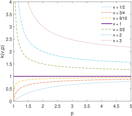
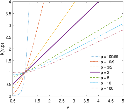
?figurename? 1: The radial exponent $k(\nu,p)$ as function of $\nu$ and $p$.

Figure 1 shows the radial exponent $k(\nu,p)$ for some $\nu$ and $p$. Curves for $\nu<1$ approaches zero as $p\to 1$ and 1 as $p\to\infty$. Curves for $\nu>1$ approaches infinity as $p\to 1$ and $\nu^{2}/(2\nu-1)$ as $p\to\infty$. Moreover, $k(\nu,p)\to\infty$ as $\nu\to\infty$, reflecting the case when the sector $\mathcal{S}_{\nu}$ approaches a line. The asymptotic behaviour in this case is $k(\nu,p)=\frac{p\nu}{2(p-1)}+O(1)$ which is in agreement with a related result in [34]. Further, the case $k(1/2,p)$ captures the rate at which the $p$-harmonic measure (or a positive $p$-harmonic function) vanish at a halfline because $\mathcal{S}_{1/2}=\mathbb{R}^{2}\setminus\{(r,\phi):\phi=\pi\}$. Furthermore, we retrieve the known results in the classical cases $k(\nu,2)=\nu$ and $k(1,p)=1,$ of which the first corresponds to the harmonic measure $(p=2)$ and in the second $\mathcal{S}_{\nu}$ is a halfplane.

When $p=2$ the $p$-harmonic measure coincides with the famous harmonic measure and our result, expressed in probabilistic terms, answers the question; what is the probability that a Brownian motion started at $x\in\mathcal{S}_{\nu}$ will first hit the part of the boundary consisting of the arc $\partial B(0,R)\cap\mathcal{S}_{\nu}$? Our estimate in (1.4) implies that the probability is comparable to $(|x|/R)^{\nu}$.

Our estimates for the $p$-harmonic measure imply local growth estimates for $p$-sub- and $p$-superharmonic functions vanishing on a fraction of a domain contained in, or containing, a sector. Indeed, we conclude that solutions must vanish at the same rate as $|x|^{k(\nu,p)}$ as $x$ approaches the apex (Corollary 5.1). Similar growth estimates where proved in the setting of $C^{1,1}$-domains in [7] and for wider classes of equations and other geometric settings in [37, 38, 39, 45, 46, 5, 48]. An immediate consequence of Corollary 5.1 is the boundary Harnack inequality for $p$-harmonic functions in planar sectors, see (5.3). For $\nu\neq\frac{1}{2}$ such result is already well known by [37, 39] since then $\mathcal{S}_{\nu}$ is a Lipschitz domain.

Consider a domain $\Omega\subset\mathbb{R}^{2}$ having a sharp outwardly pointed cusp with apex $w$ and let $u$ be a $p$-subharmonic function taking nonpositive boundary values in a neighborhood of $w$. Using Corollary 5.1 we prove that then the rate of convergence to zero, as $x$ approaches the apex, is faster than any power of $|x-w|$, i.e. for any $N>0$ it holds that

$$\underset{x\in\Omega}{\underset{x\to w}{\limsup}}\;\frac{u(x)}{|x-w|^{N}}\leq 0,$$

which is a result proved already in [34, Theorem 3]. Consider now instead a domain $\Omega\subset\mathbb{R}^{2}$ having a sharp inwardly pointed cusp at $w$, and let $v$ be a $p$-superharmonic function taking nonnegative boundary values in a neighborhood of $w$. In this case we prove that the rate of convergence to zero, as $x$ approaches the apex, is slower than $|x-w|^{\frac{p-1}{p}}$, i.e.,

$$\underset{x\in\Lambda}{\underset{x\to w}{\limsup}}\;\frac{u(x)}{|x-w|^{N}}>0,\quad\text{where}\quad\Lambda=\{x\in\Omega:d(x,\partial\Omega)\geq|x-w|\}.$$

The $p$-harmonic measure has a probabilistic interpretation in terms of the zero-sum two-player game tug-of-war, see [52] and [53], in which also estimates for $p$-harmonic measure are proved, e.g. for porous sets. Further results in the literature include [49] who proved estimates for $p$-harmonic measures in the plane, which, together with a result in [27], yield properties of the $p$-Green function. Estimates for the $p$-harmonic measure of a small spherical cap and of small axially symmetric sets are proved in [20, 21], and in [22] estimates for the $p$-harmonic measure is given of the part of the boundary of an infinite slab outside a cylinder. In [46] estimates of $p$-harmonic measure, $n-m<p\leq\infty$, for sets in $\mathbb{R}^{n}$ which are close to an $m$-dimensional hyperplane, $0\leq m\leq n-1$ are proved, and in [42] it is proved that the $p$-harmonic measure in $\mathbb{R}_{+}^{n}$ of a ball of radius $0<\delta\leq 1$ in $\mathbb{R}^{n-1}$ is bounded above and below by a constant times $\delta^{\alpha}$, and explicit estimates for $\alpha$ are given. For more on possible applications of $p$-harmonic measure, see e.g. [25, Chapter 11 and Chapter 14] including Phragmen–Lindelöfs theorem and the study of quasiregular mappings.

In Section 6 we use the estimates in Theorem 4.1 to prove Theorem 6.1 which is an extended version of the classical result of Phragmén–Lindelöf [55]. In particular, suppose that $u$ is p-subharmonic in an unbounded planar domain $\Omega$ contained in the sector $\mathcal{S}_{\nu}$ and suppose that $\limsup_{z\to\partial\Omega}u(z)\leq 0$. Then either $u\leq 0$ in the whole of $\Omega$ or it holds that

$$\liminf_{R\to\infty}\left(\frac{1}{R^{k(\nu,p)}}\sup_{\partial B(0,R)\cap\Omega}u\right)>0,$$

where $k(\nu,p)$ is as in (1.5). When $\Omega\equiv\mathcal{S}_{\nu}$, the above growth rate is sharp. We remark that when $\nu=1$ the sector $\mathcal{S}_{\nu}$ is a halfplane and $k(1,p)=1$; thus we retrieve the classical result that $p$-subharmonic functions must grow at least as fast as the distance to the boundary [40].

In connection with the above Phragmén-Lindelöf result we also prove, for $p\in(1,\infty)$, $\nu\in(1/2,\infty)$, that positive $p$-harmonic functions in $\mathcal{S}_{\nu}$, vanishing on $\partial\mathcal{S}_{\nu}$, are unique (modulo normalization), see Theorem 7.1. The proof of this result uses scaling arguments and a boundary estimate from [39].

Being a generalization of maximum principles to unbounded domains the Phragmén-Lindelöf principle [55] is undoubtedly an important result with applications in e.g. elasticity theory [28, 56, 36]. To summarize some literature (without giving a complete list) we mention that results of [55] was extended to halfspaces of $\mathbb{R}^{n}$ in [6] and to general elliptic equations of second order in [23, 58, 26]. Uniformly elliptic equations in nondivergence form in cones were considered in [50], growth estimates of bounded solutions of quasilinear equations in [35, 30] and for elliptic equations in sectors, see [59]. Fully nonlinear equations were considered in [17, 8], the later in certain Lipschitz domains, and [32] considered fully nonlinear elliptic PDEs with unbounded coefficients and nonhomogeneous terms. Results for variable exponent $p$-Laplace-type equations can be found in [4], while infinity-harmonic functions are considered in [12, 24]. In [40], Phragmén-Lindelöf’s theorem for $n$-subharmonic functions, when the boundary is an $m$-dimensional hyperplane in $\mathbb{R}^{n}$, $0\leq m\leq n-1$ is proved. This was extended to $p$-subharmonic functions, $n-m<p\leq\infty$, in [46]. In [16] it is showed that solutions of a generalized $p$-Laplace equation in the upper halfplane, vanishing on $\{x_{n}=0\}$, equals $u(x)=x_{n}$ (modulo normalization), while the growth of solutions of the minimal surface equation over domains containing a halfplane was considered in [43]. A Phragmén-Lindelöf theorem for a mixed boundary value problem for quasilinear elliptic equations of $p$-Laplace type in an open infinite circular half-cylinder was proved in [15]. The spatial behavior of solutions of the Laplace equation on a semi-infinite cylinder with dynamical nonlinear boundary conditions was investigated in [36]. In halfspaces of $\mathbb{R}^{n}$, growth estimates for subsolutions of fully nonlinear nonhomogeneous PDEs was characterized in terms of solutions to certain ordinary differential equations in [47]. Using this characterization, several Phragmen-Lindelöf-type results were derived, e.g. a sharp theorem for the variable exponent $p$-Laplace equation, and also sharp results for equations allowing for sublinear growth in the gradient. Phragmén-Lindelöf theorems for plurisubharmonic functions on cones were proved in [51] while $k$-Hessian equations with lower order terms were considered in [14]. The present paper complements the above by giving the sharp exponent $k(\nu,p)$ explicitly in case of positive $p$-harmonic functions in planar sectors.

In Section 2 we summarize some well known basic definitions and properties of solutions to the $p$-Laplace equation and in Sections 3 and 9 we summarize and prove properties on explicit $p$-harmonic functions in planar sectors. Using these results we state and prove our estimates of $p$-harmonic measure in Section 4, while in Section 5 we give Corollaries for $p$-sub- and $p$-superharmonic functions. Sections 6 and 7 is devoted to Phragmen-Lindelöfs theorem and uniqueness of $p$-harmonic functions in sectors, respectively. We end the paper by showing in Section 8 that in the case of infinity-harmonic measure and infinity-harmonic functions then most of our results extend to symmetric $n$-dimensional domains, $n>2$.

2 Preliminaries

In this section we state some basic definitions and results for $p$-harmonic measure and $p$-harmonic functions needed later. By $\Omega$ we denote a domain, that is, an open connected set. For a set $E\subset\mathbb{R}^{n}$ we let $\overline{E}$ denote the closure and $\partial E$ the boundary. Further, $d(x,E)$ denotes the Euclidean distance from $x\in\mathbb{R}^{n}$ to $E$, and $B(z,r)=\{x\in\mathbb{R}^{2}:d(x,z)<r\}$ denotes the open ball with radius $r$ and center $z$. By $c$ we denote a constant $\geq 1$, not necessarily the same at each occurrence, depending only on $\nu$ and $p$ if nothing else is mentioned. Moreover, $c(a_{1},a_{2},\dots,a_{k})$ denotes a constant $\geq 1$, not necessarily the same at each occurrence, depending only on $a_{1},a_{2},\dots,a_{k}$.

We proceed with defining weak and viscosity solutions and $p$-harmonicity. If $p\in(1,\infty)$, we say that $u$ is a (weak) subsolution (supersolution) to the $p$-Laplacian in a domain $\Omega$ provided $u\in W_{loc}^{1,p}(\Omega)$ and

$$\int\limits_{\Omega}|\nabla u|^{p-2}\,\langle\nabla u,\nabla\theta\rangle\,dx\leq(\geq)\,0,$$

whenever $\theta\in C^{\infty}_{0}(\Omega)$ is non-negative. A function $u$ is a (weak) solution of the $p$-Laplacian if it is both a subsolution and a supersolution. Here, and in the sequel, $W^{1,p}(\Omega)$ is the Sobolev space of those $p$-integrable functions whose first distributional derivatives are also $p$-integrable, and $C^{\infty}_{0}(\Omega)$ is the set of infinitely differentiable functions with compact support in $\Omega$. If $p=\infty$, the equation is no longer of divergence form and therefore the above definition needs to be replaced. We use instead the notion of viscosity solutions. Here, and in the sequel, $\Delta_{\infty}$ is the $\infty$-Laplace operator defined in (1.2).

An upper semicontinuous function $u:\Omega\rightarrow\mathbb{R}$ is a (viscosity) subsolution of the $\infty$-Laplacian in $\Omega$ provided that for each function $\psi\in C^{2}(\Omega)$ such that $u-\psi$ has a local maximum at a point $x_{0}\in\Omega$, we have $\Delta_{\infty}\psi(x_{0})\geq 0$. A lower semicontinuous function $u:\Omega\rightarrow\mathbb{R}$ is a (viscosity) supersolution of the $\infty$-Laplacian in $\Omega$ provided that for each function $\psi\in C^{2}(\Omega)$ such that $u-\psi$ has a local minimum at a point $x_{0}\in\Omega$, we have $\Delta_{\infty}\psi(x_{0})\leq 0$. A function $u:\Omega\rightarrow\mathbb{R}$ is a (viscosity) solution of the $\infty$-Laplacian if it is both a subsolution and a supersolution.

If $u$ is an upper semicontinuous subsolution to the $p$-Laplacian in $\Omega$, $p\in(1,\infty]$, then we say that $u$ is $p$-subharmonic in $\Omega$. If $u$ is a lower semicontinuous supersolution to the $p$-Laplacian in $\Omega$, $p\in(1,\infty]$, then we say that $u$ is $p$-superharmonic in $\Omega$. If $u$ is a continuous solution to the $p$-Laplacian in $\Omega$, $p\in(1,\infty]$, then $u$ is $p$-harmonic in $\Omega$.

We note that for the $p$-Laplacian, $1<p<\infty$, weak solutions are also viscosity solutions (defined as above but with $\Delta_{\infty}$ replaced by $\Delta_{p}$); see [31, Theorem 1.29]. Moreover, under suitable assumptions, an $\infty$-harmonic function is the uniform limit of a sequence of $p$-harmonic functions as $p\to\infty$; see [29]. For more on weak solutions, viscosity solutions, $p$-harmonicity and $p$-superharmonicity, see for instance [25] and [19].

We will make use of the nowadays well known basic properties of $p$-harmonic functions:

Lemma 2.1

Let $p\in(1,\infty]$ and suppose that $u$ is $p$-superharmonic and that $v$ is $p$-subharmonic in a bounded domain $\Omega\subset\mathbb{R}^{n}$. If

$$\limsup_{z\to w}v(z)\leq\liminf_{z\to w}u(z)$$

for all $w\in\partial\Omega$, and if both sides of the above inequality are not simultaneously $\infty$ or $-\infty$, then $v\leq u$ in $\Omega$.

Proof. If $p\in(1,\infty)$ then this follows from [25, Theorem 7.6]. For the case $p=\infty$ this was first proved in [29, Theorem 3.11]. A shorter proof was later given in [9].  

Lemma 2.2

Let $\Omega\subset\mathbb{R}^{n}$ be a domain, $p\in(1,\infty]$ and assume that $u$ is a $p$-harmonic function in $\Omega$. Let $k\in\mathbb{R}$ and $z\in\mathbb{R}^{n}$. Then $\hat{u}$ is $p$-harmonic in some $\widetilde{\Omega}\in\mathbb{R}^{n}$, in either of the following cases:

$$(i)\;\hat{u}=ku,\quad(ii)\;\hat{u}=u(x+z),\quad(iii)\;\hat{u}=u(kx).$$

Proof. Follows by standard calculations.  

Lemma 2.3

Let $p\in(1,\infty]$, $w\in\mathbb{R}^{n}$, $r\in(0,\infty)$ and suppose that $u$ is a positive $p$-harmonic function in $B(w,2r)$. Then there exists a constant $c\in(1,\infty]$, depending only on $p$ and $n$, such that

$$\sup_{B(w,r)}u\leq c\inf_{B(w,r)}u\text{.}$$

Proof. For the case $p\in(1,\infty)$, see e.g. [33]. For the case $p=\infty$ the result follows by taking the limit $p\to\infty$ in the former case, see [41].  

The following well known estimate tells that $p$-harmonic functions are Hölder continuous up to the boundary in the setting of the rather general class of non-tangentially accessible (NTA) domains. We will only apply the result in smooth planar domains, and refer the interested reader to e.g. [44, Chapter 1.6] for a definition of NTA-domains.

Lemma 2.4

Assume that $\Omega\subset\mathbb{R}^{n}$ is an NTA-domain with constant $M$, let $w\in\partial\Omega$, $0<r<r_{0}$ and suppose that $u$ is a positive $p$-harmonic function in $\Omega\cap B(w,2r)$, continuous on $\overline{\Omega}\cap B(w,2r)$ with $u=0$ on $\partial\Omega\cap B(w,2r)$. Then there exist $c$ and $\alpha\in(0,1]$, depending only on $M$, $n$ and $p$, such that

$$|u(x)-u(y)|\leq c\left(\frac{|x-y|}{r}\right)^{\alpha}\sup_{B(w,2r)\cap\Omega}u,$$

whenever $x,y\in B(w,r)\cap\Omega$.

Proof. By observing that $\Omega$ is $p$-regular by the NTA-assumption, the lemma follows by the same arguments as in [25, Theorem 6.44, Lemma 6.47].  

The following Lemma states that any positive $p$-harmonic function, vanishing on a portion of the boundary of a $C^{1,1}$-domain, must vanish at the same rate as the distance to the boundary. The right inequality in Lemma 2.5 – which is an immediate consequence of the left inequality – is usually referred to as a boundary Harnack inequality and states that any two $p$-harmonic functions, vanishing on the boundary, must vanish at the same rate.

Lemma 2.5

Let $\Omega\in\mathbb{R}^{n}$ be a $C^{1,1}$-domain, or equivalently a domain satisfying the ball condition with radius $r_{b}$, $p\in(1,\infty]$, $n\geq 2$, $w\in\partial\Omega$ and $0<r<r_{b}$. Suppose that $u$ and $v$ are positive $p$-harmonic functions in $\Omega\cap B(w,r)$, satisfying $u=0=v$ on $\partial\Omega\cap B(w,r)$. Then there exists $c=c(n,p)$ such that

$$c^{-1}\frac{d(x,\partial\Omega)}{r}\leq\frac{u(x)}{u(a_{r}(w))}\leq c\frac{d(x,\partial\Omega)}{r}\quad\text{and}\quad c^{-1}\frac{u(a_{r}(w))}{v(a_{r}(w))}\leq\frac{u(x)}{v(x)}\leq c\frac{u(a_{r}(w))}{v(a_{r}(w))},$$

whenever $x\in\Omega\cap B(w,r/c)$. Here, $a_{r}(w)$ is a point in $\Omega$ satisfying $d(a_{r}(w),w)=r/c$ and $d(a_{r}(w),\partial\Omega)=r/c$.

Proof. For $p\in(1,\infty)$ we refer to [7, Lemma 3.1 and Lemma 3.3]. See also [37, 38, 39] for similar as well as stronger estimates in more general geometries. When $p=\infty$ the proof is similar, but then the comparison argument uses cones (which are $\infty$-harmonic) in place of the function $\phi_{p}(x)$ defined on [7, page 286], and therefore the exterior ball condition is not needed. See also [13] for the case $p=\infty$.   

3 Explicit $p$-harmonic functions in sectors

In this section we are gonna prove the following Lemma, which is similar to [49, Lemma 4.1], using some explicit $p$-harmonic functions derived in [1], [2], [3] and [54]. The result will be of crucial importance when we prove our main results in Sections 4-8.

Lemma 3.1

Let $p\in(1,\infty]$ and $\nu\in[\frac{1}{2},\infty)$. Then there exists a positive $p$-harmonic function $u_{\nu,p}:\mathcal{S}_{\nu}\rightarrow\mathbb{R}$ of the form $u_{\nu,p}(x)=r^{k}f_{\nu,p}(\phi)$, where the exponent $k=k(\nu,p)$ is given by (1.5). The exponent $k$ is non-decreasing in $\nu$, increasing in $p$ for $\nu\in[1/2,1)$, and decreasing in $p$ for $\nu>1$. Moreover, the function $f_{\nu,p}(\phi)$ is continuous, differentiable and satisfies

• $f_{\nu,p}(\pm\frac{\pi}{2\nu})=f^{\prime}_{\nu,p}(0)=0$,

• $0\leq f_{\nu,p}(\phi)\leq 1,\;|f^{\prime}_{\nu,p}(\phi)|\leq c$ when $\phi\in[-\frac{\pi}{2\nu},\frac{\pi}{2\nu}]$,

• $|f_{\nu,p}(\phi)|\geq c^{-1}$ when $\phi\in[-\frac{\pi}{4\nu},\frac{\pi}{4\nu}]$ and $|f^{\prime}_{\nu,p}(\phi)|\geq c^{-1}$ when $\phi\in[-\frac{\pi}{2\nu},\frac{\pi}{2\nu}]\setminus[-\frac{\pi}{4\nu},\frac{\pi}{4\nu}]$.

Proof. We begin by noting that standard calculations yield (see Appendix 9.3) $dk/d\nu\geq 0$ whenever $\nu\in[\frac{1}{2},\infty)$ and $p\in(1,\infty]$. Moreover, $dk/dp>0$ for $\nu\in[1/2,1)$, and $dk/dp<0$ for $\nu>1$, whenever $p\in(1,\infty)$. The rest of the proof is split into four different cases; $p=2$, $2<p$, $p=\infty$ and $1<p<2$.

Case 1: $p=2$.

In this case (1.1) reduces to the Laplace equation which yields, in polar coordinates,

$$u_{rr}+\frac{1}{r}u_{r}+\frac{1}{r^{2}}u_{\phi\phi}=0.$$

Thus, the solution $u(r,\phi)=r^{\nu}\cos(\nu\phi)$ has the desired properties since $k(\nu,p)=\nu$.

Case 2: $2<p<\infty$.

In polar coordinates the $p$-Laplace equation, with $b=1/(p-2)$, $p\neq 2$, yields (see Appendix 9.1 for a derivation),

$$\left(b+1\right)u_{r}^{2}u_{rr}+\frac{b}{r^{2}}\left(u_{rr}u_{\phi}^{2}+u_{r}^{2}u_{\phi\phi}\right)+\frac{(b+1)}{r^{4}}u_{\phi}^{2}u_{\phi\phi}+\frac{b}{r}u_{r}^{3}+\frac{(b-1)}{r^{3}}u_{r}u_{\phi}^{2}+\frac{2}{r^{2}}u_{r}u_{\phi}u_{r\phi}=0.$$ (3.1)

We are searching for solutions of the form $u(r,\phi)=r^{k}f(\phi)$, where $f(\phi)\in\mathcal{C}^{2}$ and $k$ are to be determined. Inserted in 3.1 we obtain

$$\left[\left(b+1\right)(f^{\prime})^{2}+bk^{2}f^{2}\right]f^{\prime\prime}+\left(2k+bk-1\right)kf(f^{\prime})^{2}+\left(bk+k-1\right)k^{3}f^{3}=0.$$ (3.2)

Equation (3.2) can be solved (for details check [2, Lemma 2]) to yield

$$f_{\nu,p}(\phi)=c\left(1-\frac{\cos^{2}\theta_{\nu,p}(\phi)}{ak}\right)^{\frac{k-1}{2}}\cos\theta_{\nu,p}(\phi),$$ (3.3)

where $a=(p-1)/(p-2)$ and $\theta_{\nu,p}$ is a certain continuous, strictly increasing function of $\phi$ and $c=c(\nu,p)$ is chosen so that $0\leq f_{\nu,p}\leq 1$. When $|\phi|<\frac{\pi}{2\nu}$, we have (See Appendix 9.3),

$$\phi=\theta_{\nu,p}(\phi)-\left(1-\frac{1}{k}\right)\frac{\sqrt{ak}}{\sqrt{ak-1}}\left[\arctan\left(\lambda_{\nu,p}\tan\frac{\theta_{\nu,p}(\phi)}{2}\right)+\arctan\left(\frac{1}{\lambda_{\nu,p}}\tan\frac{\theta_{\nu,p}(\phi)}{2}\right)\right],$$ (3.4)

where $\lambda_{\nu,p}=\frac{\sqrt{ak-1}}{\sqrt{ak}+1}$. The function $\theta_{\nu,p}$ is chosen so that it maps the interval $[\frac{-\pi}{2\nu},\frac{\pi}{2\nu}]$ to $[-\frac{\pi}{2},\frac{\pi}{2}]$, and this condition determines the radial exponent $k$. More precisely, the condition that determines $k$ is given by

$$\frac{\pi}{\nu}=\phi\left(\frac{\pi}{2}\right)-\phi\left(-\frac{\pi}{2}\right)=\pi\left(1-\left(1-\frac{1}{k}\right)\frac{\sqrt{ak}}{\sqrt{ak-1}}\right).$$

Solving for $k=k(\nu,p)$ we obtain the exponent given by (1.5) in the introduction. Moreover, $f_{\nu,p}\left(\pm\frac{\pi}{2\nu}\right)=0$ and $ak>1$ implying $f_{\nu,p}(\phi)>0$ for $|\phi|<\frac{\pi}{2\nu}$.

We also need to estimate the derivative of $f_{\nu,p}$. Differentiation of $f_{\nu,p}$ in (3.3) and simplifying (see [2] page 143, and/or Appendix 9.4), yield

$$f_{\nu,p}^{\prime}(\phi)=-k\,c\left(1-\frac{\cos^{2}\theta_{\nu,p}(\phi)}{ak}\right)^{\frac{k-1}{2}}\sin\theta_{\nu,p}(\phi).$$ (3.5)

Since $ak>1$ we have that $|f_{\nu,p}^{\prime}(\phi)|\leq c(\nu,p)$ for all $\phi\in[-\frac{\pi}{2\nu},\frac{\pi}{2\nu}]$. Also $f_{\nu,p}^{\prime}(\phi)=0$ will only occur when $\theta=n\pi$, $n\in\mathbb{Z}$, corresponding to $\phi=\frac{n\pi}{\nu}$. Hence the only place where $f_{\nu,p}^{\prime}$ is zero in $\mathcal{S}_{\nu}$ is in the radial direction along $\phi=0$. It follows that we can conclude, by continuity of $f^{\prime}_{\nu,p}$ which holds since $ak>1$, the existence of a constant $c=c(\nu,p)$ such that $|f^{\prime}_{\nu,p}(\phi)|\geq c^{-1}$ whenever $\phi\in[-\frac{\pi}{2\nu},\frac{\pi}{2\nu}]\setminus[-\frac{\pi}{4\nu},\frac{\pi}{4\nu}]$. It also follows that $f_{\nu,p}(\phi)\geq c^{-1}$ whenever $\phi\in[-\frac{\pi}{4\nu},\frac{\pi}{4\nu}]$. The proof when $2<p<\infty$ is complete.

Case 3: $p=\infty$.

Letting $a=1$ when $p=\infty$, the function from Case 2 is immediately extended to the case when $p=\infty$. Indeed, in this case the separation equation (3.2) boils down to

$$(f^{\prime})^{2}f^{\prime\prime}+\left(2k-1\right)kf(f^{\prime})^{2}+\left(k-1\right)k^{3}f^{3}=0,$$ (3.6)

which has solution

$$f_{\nu,\infty}(\phi)=c\left(1-\frac{\cos^{2}\theta(\phi)}{k}\right)^{\frac{k-1}{2}}\cos\theta(\phi)$$

with radial exponent

$$k(\nu,\infty)=\left\{\begin{array}[]{ll}1&\text{when}\quad\frac{1}{2}\leq\nu\leq 1,\\ \frac{\nu^{2}}{2\nu-1}&\text{when}\quad 1\leq\nu.\end{array}\right.$$

This case is studied in detail in [1] and $f_{\nu,\infty}$ is infinitely differentiable on $[-\frac{\pi}{2\nu},0)\cup(0,\frac{\pi}{2\nu}]$ and differentiable at $\phi=0$. It follows that $u_{\nu,\infty}=r^{k}f_{\nu,\infty}$ satisfies the required conditions, except that it is not immediate that the function is $\infty$-harmonic in the viscosity sense in the entire sector. This is because at points where $f_{\nu,\infty}^{\prime}(\phi)=0$ we have $f^{\prime\prime}_{\nu,\infty}(\phi)=-\infty$, which can be seen from (3.6), and $f_{\nu,\infty}(\phi)$ is thus not $C^{2}$ there. For $\nu=1$, it was shown in [11, appendix I] that $r^{-1/3}f_{1,\infty}$ is indeed $\infty$-harmonic in the viscosity sense. However, the exact same proof works for all $\nu\geq\frac{1}{2}$; or more generally, for $\infty$-harmonic functions with polar representation $r^{k}f(\phi)\geq 0$, with $k\cdot(1-k)\leq 0$ and where $f\in C^{1}$ is $C^{2}$ for $\phi\neq 0$, has a local maximum at $\phi=0$ and satisfies $\lim_{\phi\to 0}f^{\prime\prime}(\phi)=-\infty$. To complete the proof of the lemma when $p=\infty$ we observe that statements $i)-iii)$ follow in a similar way as in the case $2<p<\infty$.

Case 4: $1<p<2$.

We are going via a stream function technique to handle this situation. Indeed, we will use the stream function for the case $2<p<\infty$ to find our desired solution for $1<p<2$. We begin by the following lemma from [3] for which we present a proof in Appendix 9.5.

Lemma 3.2

Let $u(r,\phi)=r^{k}f(\phi)$ be $p$-harmonic in sector $\mathcal{S}_{\nu}$, $k>0$, and $2<p<\infty$. Then there exists a $q$-harmonic stream function $v(r,\phi)=r^{\lambda}g(\phi)$ in $\mathcal{S}_{\nu}$, where $\lambda=(p-1)(k-1)+1$, $q=p/(p-1)$, and

$$g(\phi)=-\dfrac{1}{\lambda}f^{\prime}(\phi)\left(k^{2}f(\phi)^{2}+f^{\prime}(\phi)^{2}\right)^{\frac{p-2}{2}}.$$

The function $g(\phi)$ is periodic whenever $f(\phi)$ is.

To apply Lemma 3.2 it is convenient to view the $p$-values at hand as conjugate to those in Case 2, i.e. when $2<p<\infty$. Hence, fix $q\in(1,2)$ and denote the conjugate index by $p=q/(q-1)\in(2,\infty)$. Substituting $p=q/(q-1)$ into $\lambda=(p-1)(k-1)+1$ and exercising some algebra gives

$$\lambda\left(\nu,\frac{q}{q-1}\right)=\frac{(\nu-1)\sqrt{(1-2\nu)(q-2)^{2}+\nu^{2}q^{2}}+(2-q)(1-2\nu)+\nu^{2}q}{2(q-1)(2\nu-1)}=k(\nu,q).$$

Therefore, the same expression for the exponent continues to hold also for $q\in(1,2)$. Next, we consider the function $f_{\nu,p}$, defined in Case 2, in the extended domain $\phi\in[\frac{-\pi}{2\nu},\frac{\pi}{\nu}]$. Note that such extension is immediate (interpreting $\lim_{\underset{\theta\in(-\pi,\pi)}{\theta\to\pm\pi}}\phi(\theta)=\pm\frac{\pi}{\nu}$ in expression (3.4)) and that the function $(r,\phi)\to r^{k}f_{\nu,p}(\phi)$ is still $p$-harmonic in the extended domain. Now, let $\bar{u}_{\nu,p}(x_{1},x_{2})=r^{k}f_{\nu,p}(\phi)$ for $r>0$ and $\phi\in[0,\frac{\pi}{\nu}]$. As we shall see, the stream function of $\bar{u}_{\nu,p}$ is, up to rotation, the desired function. In particular, put $f_{\nu,p}(\phi)$ from (3.3) and $f^{\prime}_{\nu,p}(\phi)$ from (3.5) in Lemma 3.2, using $p=q/(q-1)$ and some algebra we arrive at

$$g_{\nu,q}(\phi)=\frac{k\left(\nu,p\right)^{p-1}}{\lambda\left(\nu,\frac{q}{q-1}\right)}\left(1-\frac{\cos^{2}(\theta)}{ak(\nu,p)}\right)^{\frac{\left(k(\nu,p)-1\right)\left(p-1\right)}{2}}\sin(\theta)\\ =\frac{k(\nu,p)^{p-1}}{k(\nu,q)}\left(1-\frac{\cos^{2}(\theta)}{\frac{1}{2-q}\left(\lambda(\nu,\frac{q}{q-1})(q-1)+2-q\right)}\right)^{\frac{\lambda\left(\nu,\frac{q}{q-1}\right)-1}{2}}\sin(\theta)\\ \ =\frac{k(\nu,\frac{q}{q-1})^{\frac{1}{q-1}}}{k(\nu,q)}\left(1-\frac{\cos^{2}(\theta)}{\frac{q-1}{2-q}k(\nu,q)+1}\right)^{\frac{k(\nu,q)-1}{2}}\sin(\theta).$$

Similarly, from the proof of Lemma 9.2 in Appendix 9.5 we get

$$g_{\nu,q}^{\prime}(\phi)=k(\nu,p)f_{\nu,p}(\phi)\left(k(\nu,p)^{2}f_{\nu,p}(\phi)^{2}+f^{\prime}_{\nu,p}(\phi)^{2}\right)^{\frac{p-2}{2}}\\ =k\left(\nu,\frac{q}{q-1}\right)^{\frac{1}{q-1}}\left(1-\frac{\cos^{2}(\theta)}{\frac{q-1}{2-q}k(\nu,q)+1}\right)^{\frac{k(\nu,q)-1}{2}}\cos(\theta).$$

Now since $\lim_{\nu\to 1/2}k(\nu,q)=\frac{q-1}{q}\leq k\left(\nu,q\right)$ and $0<\frac{(q-1)^{2}}{(2-q)q}$ approaches zero only when $q\to 1$, we conclude

$$0<\kappa<1-\frac{\cos^{2}(\theta)}{\frac{q-1}{2-q}k(\nu,q)+1}<1,$$ (3.7)

whenever $q\in(1,2)$, where $\kappa$ depends only on $p$, and can be taken to be increasing in $p$. Therefore, $|g_{\nu,q}|\leq c(\nu,p)$, $|g^{\prime}_{\nu,q}|\leq c(\nu,p)$.

Now let $\tilde{f}_{\nu,p}(\phi)=g_{\nu,q}\left(\phi+\frac{\pi}{2\nu}\right)$. Then, since the $p$-Laplace equation is invariant under rotations (Lemma 2.2), $u(x_{1},x_{2})=r^{k(\nu,q)}\tilde{f}_{\nu,p}(\phi)$ is a positive $q$-harmonic function in $\mathcal{S}_{\nu}$ satisfying the desired boundary conditions. Moreover, $\tilde{f}^{\prime}_{\nu,q}(\phi)$ is continuous by (3.7) and only zero for $\phi=0$ when restricting to $\mathcal{S}_{\nu}$. Therefore, we conclude that $|\tilde{f}^{\prime}_{\nu,p}(\phi)|\geq c^{-1}$ whenever $\phi\in[-\frac{\pi}{2\nu},\frac{\pi}{2\nu}]\setminus[-\frac{\pi}{4\nu},\frac{\pi}{4\nu}]$. It also follows that $\tilde{f}_{\nu,p}(\phi)\geq c^{-1}$ whenever $\phi\in[-\frac{\pi}{4\nu},\frac{\pi}{4\nu}]$. This completes the proof for the case $1<p<2$ and hence also the proof of Lemma 3.1.  

4 Estimates for $p$-harmonic measure

We will now state our growth estimate for $p$-harmonic measure in planar sectors. We postpone the proof to the end of the section.

Theorem 4.1

Suppose that $p\in(1,\infty]$, $\nu\in[1/2,\infty)$, $R>0$ and $\mathcal{S}_{\nu}\subset\mathbb{R}^{2}$ is the sector defined in (1.3). Let $k(\nu,p)$ be the exponent in (1.5) and let $\omega_{p}(x)$ be the $p$-harmonic measure of $\partial B(0,R)\cap\mathcal{S}_{\nu}$ at $x$ with respect to $B(0,R)\cap\mathcal{S}_{\nu}$. Then there exists $c=c(\nu,p)$ such that

$$c^{-1}\,\left(\frac{|x|}{R}\right)^{k(\nu,p)}\,\leq\omega_{p}(x)\,\leq c\,\left(\frac{|x|}{R}\right)^{k(\nu,p)},$$

whenever $x\in B(0,R)\cap\mathcal{S}_{2\nu}$.

We remark that the upper bound of Theorem 4.1 holds also in $B(0,R)\cap\mathcal{S}_{\nu}$ which follows from a comment in the end of the proof. By Harnack’s inequality in Lemma 2.3 the lower bound also holds for any $x\in B(0,R)\cap\mathcal{S}_{\nu}$ but then the constant depends on the distance from $x$ to $\partial\mathcal{S}_{\nu}$. Furthermore, by carefully tracing constants in the proof it can be shown that the final constant $c(\nu,p)$ in Theorem 4.1 can be chosen independent of $p$ if $p$ is large, and the case $p=\infty$ in Theorem 4.1 can be derived by taking the limit of the estimates for finite $p$.

For a final remark, let $\bar{\omega}_{p}$ be the $p$-harmonic measure of $\partial B(0,R)\cap\mathcal{S}_{2\nu}$ at $x$ with respect to $B(0,R)\cap\mathcal{S}_{\nu}$. Then there exists $c=c(\nu,p)$ such that

$$c^{-1}\,\left(\frac{|x|}{R}\right)^{k(\nu,p)}\,\leq\bar{\omega}_{p}(x)\,\leq c\,\left(\frac{|x|}{R}\right)^{k(\nu,p)},$$ (4.1)

whenever $x\in B(0,R/2)\cap\mathcal{S}_{2\nu}$. To see that (4.1) holds we first observe that the upper bound is immediate from the comparison principle and Theorem 4.1. To prove the lower bound we apply the boundary Harnack inequality in Lemma 2.5 to $\omega_{p}$ and $\bar{\omega}_{p}$ near the points of intersection of $\partial B(0,R/2)$ and $\mathcal{S}_{\nu}$ and conclude that both functions vanishes at the same rate in a neighbourhood of these points. This, together with an application of Hölder continuity up to the boundary (Lemma 2.4) near the point $(r,\phi)=(R,0)$ and Harnack’s inequality toward the points of intersections, applied to $\bar{\omega}_{p}$, ensures $c(\nu,p)\bar{\omega}_{p}\geq\omega_{p}$ on $\partial B(0,R/2)\cap\mathcal{S}_{\nu}$. We now apply the comparison principle in $B(0,R/2)\cap\mathcal{S}_{\nu}$ and Theorem 4.1 to obtain the lower bound.

Proof of Theorem 4.1. Let $u(x)=u(r,\phi)=r^{k}f_{\nu,p}(\phi)$ be the $p$-harmonic function from Lemma 3.1 and observe that $R^{-k}u(x)$ is $p$-subharmonic in $\mathcal{S}_{\nu}$ with boundary values $R^{-k}u(x)=0$ on $\partial\mathcal{S}_{\nu}$ and $R^{-k}u(x)\leq 1$ on $\partial B(0,R)\cap\mathcal{S}_{\nu}$, see $ii)$ in Lemma 3.1. This together with Definition 1.1 of the $p$-harmonic measure ensure that

$$\limsup_{x\rightarrow y}{R^{-k}u(x)}\leq\liminf_{x\rightarrow y}{\omega_{p}(x)},\quad\forall y\in\partial(B(0,R)\cap\mathcal{S}_{\nu}),$$

and hence by the comparison principle (Lemma 2.1) we obtain

$$R^{-k}u(x)\leq\omega_{p}(x),\quad\forall\,x\in B(0,R)\cap\mathcal{S}_{\nu}.$$

Lemma 3.1 $iii)$ now implies

$$\omega_{p}(x)\geq R^{-k}u(x)=R^{-k}r^{k}f_{\nu,p}(\phi)=\left(\frac{|x|}{R}\right)^{k}f_{\nu,p}(\phi)\geq\frac{1}{c}\left(\frac{|x|}{R}\right)^{k},$$ (4.2)

whenever $x\in B(0,R)\cap\mathcal{S}_{2\nu}$, which establishes the lower bound.

?figurename? 2: Geometry in the proof of Theorem 4.1.

We will now prove the upper bound. As $\omega_{p}\approx 1$ at points near the intersections of $\partial B(0,R)$ and $\partial\mathcal{S}_{\nu}$ where $u\approx 0$ we chose to make comparison on a smaller domain not including these points. Let $z\in\partial\mathcal{S}_{\nu}$ be the midpoint on the line from the origin to $(R,-\frac{\pi}{2\nu})$. By the upper boundary growth estimate for $p$-harmonic functions in Lemma 2.5 there exists a constant $c=c(p)$ such that

$$\omega_{p}(x)\leq c\,\frac{d(x,\partial\mathcal{S}_{\nu})}{R}\,\omega_{p}\left(a_{R}(w)\right)\leq c\,\frac{d(x,\partial\mathcal{S}_{\nu})}{R}\quad\text{whenever}\quad x\in B(z,R/c)\cap\mathcal{S}_{\nu}.$$ (4.3)

Using the fact that $f_{\nu,p}^{\prime}(\phi)$ does not vanish near $\partial\mathcal{S}_{\nu}$ (Lemma 3.1 $iii)$), we also see that, for $c=c(\nu,p)$,

$$u(x)R^{-k}\geq\frac{1}{c}\frac{d(x,\partial\mathcal{S}_{\nu})}{R}\quad\text{whenever}\quad x\in B(z,R/c)\cap\mathcal{S}_{\nu}.$$ (4.4)

Inequalities (4.3) and (4.4) implies

$$\omega_{p}(x)\leq cR^{-k}u(x)\quad\text{whenever}\quad x\in B(z,R/c)\cap\mathcal{S}_{\nu}.$$ (4.5)

Next, we also see from (4.4) and continuity of $u$ that, for $c=c(\nu,p)$,

$$cR^{-k}u(\xi)\geq 1,$$ (4.6)

where $\xi=(R_{\xi},\phi_{\xi})$ is the point on the boundary of $B(z,R/c)$ with $d(\xi,\partial S_{\nu})=R/c$.

Since $u$ and $\omega_{p}$ are continuous in $\mathcal{S}_{\nu}\cap B(0,R)$ and $0<\omega_{p}<1$ in $\mathcal{S}_{\nu}\cap B(0,R)$ we conclude from (4.5) and (4.6) that

$$\limsup_{x\to y}\,\omega_{p}(x)\leq\liminf_{x\to y}\,cR^{-k}u(x),\quad\forall\,x\in\mathcal{S}_{\nu}\cap B(0,R),\,y\in\partial\Gamma.$$ (4.7)

Here, $\Gamma\subset\mathcal{S}_{\nu}$ is the open set bounded by the curve starting at the origin and reaching $z$ in the $r$-direction, then proceeding along a straight line to $\xi$ and from there to $\partial B(0,R)$ in $r$-direction, and proceeding in $\phi$-direction to the point $(R,0)$. The rest of the curve, back to the origin, is the mirror of the above curve in the line $\phi=0$ (see Figure 2). Using (4.7) and the comparison principle (Lemma 2.1) we conclude that

$$\omega_{p}(x)\leq cR^{-k}u(x),\quad\forall x\in\Gamma.$$

Since $B(0,R)\cap\mathcal{S}_{2\nu}\subset\Gamma$, at least if $|\phi_{\xi}|\geq\frac{\pi}{4\nu}$ which we may assume, it follows that

$$\omega_{p}(x)\leq cR^{-k}u(x)=cR^{-k}r^{k}f_{\nu,p}(\phi)\leq c\left(\frac{|x|}{R}\right)^{k},$$

which establishes the upper bound in $B(0,R)\cap\mathcal{S}_{2\nu}$. Observing that $B(0,R/2)\cap\mathcal{S}_{\nu}\subset\Gamma$ and that $\omega_{p}\leq 1$ we can conclude that the upper bound holds also whenever $x\in B(0,R)\cap\mathcal{S}_{\nu}$. This together with the lower bound in (4.2) completes the proof of Theorem 4.1. $\blacksquare$

We remark that in the case when $\nu\in[1/2,1]$ and $p=\infty$, giving $k(\nu,\infty)=1$, we can prove Theorem 4.1 using the fact that infinity harmonic functions obey the comparison with cones principle, see [18]. Indeed, the lower bound can be proved by making comparison with a cone function placed inside of $\mathcal{S}_{\nu}$, so that the circular base of the cone touches the boundary of $\mathcal{S}_{\nu}$ at the origin (always possible since $\nu\leq 1$). The upper bound follows by comparison with a cone function placed so that its tip is at the origin. This argument for proving an upper bound works for any $\nu\in[1/2,\infty)$ but it is optimal only when $\nu\leq 1$.

We also remark that for the cases when $p\in(1,\infty)$ and $\nu\in(\frac{1}{2},\infty)$ we may prove Theorem 4.1 by scaling and an application of the boundary Harnack inequality in Lemma 7.2 (given in Section 7 below) by taking $v(x)$ as the $p$-harmonic function in Lemma 3.1 and $u(x)$ as the $p$-harmonic measure. This works because the sector $\mathcal{S}_{\nu}$ is a Lipschitz domain as long as $\nu\neq\frac{1}{2}$.

5 Estimates for $p$-sub- and $p$-superharmonic functions

In this section we state and prove some Corollaries of Theorem 4.1 giving estimates of $p$-sub- and $p$-superharmonic functions in domains related to planar sectors.

Corollary 5.1

Suppose that $p\in(1,\infty]$, $\nu\in[1/2,\infty)$, $R>0$, $\Omega\in\mathbb{R}^{2}$ is a domain, $w\in\partial\Omega$ and that $\Omega\cap B(w,R)$ is contained in a planar sector with apex $w$ and aperture angle $\frac{\pi}{\nu}$. Let $u$ be a $p$-subharmonic function in $\Omega$, satisfying $u\leq 0$ on $\partial\Omega\cap B(w,R)$. Then

$$u(x)\leq cM\left(\frac{|x-w|}{R}\right)^{k(\nu,p)}$$ (5.1)

whenever $x\in\Omega\cap B(w,R)$, $M=\max\left\{0,\sup_{\partial B(w,R)\cap\Omega}u\right\}$ and where $c=c(\nu,p)$ is the constant in Theorem 4.1.

Suppose now instead that $\mathcal{C}_{\nu}\cap B(w,R)$ is contained in $\Omega$, where $\mathcal{C}_{\nu}$ is a cone with apex $w$ and aperture angle $\frac{\pi}{\nu}$, and that $v$ is a nonnegative $p$-superharmonic function in $\Omega$, satisfying $v\geq 0$ on $\partial\Omega\cap B(w,R)$. Then

$$c^{-1}m\left(\frac{|x-w|}{R}\right)^{k(\nu,p)}\leq v(x)$$ (5.2)

whenever $x\in B(w,R/2)\cap\mathcal{C}_{2v}$, $m=\inf_{\partial B(w,R)\cap\mathcal{C}_{2v}}v$ and where $c=c(\nu,p)$ is the constant in inequality (4.1).

Proof. We begin by proving (5.1). Thanks to Lemma 2.2 we change coordinates so that $w=(0,0)$ and the domain $\Omega$ is contained in $\mathcal{S}_{\nu}$. Let $\omega_{p}$ be the $p$-harmonic measure in Theorem 4.1. We can conclude that

$$M\omega_{p}(x)\leq cM\left(\frac{|x|}{R}\right)^{k(v,p)}$$

whenever $x\in B(0,R)\cap\Omega$ where

$$M=\max\left\{0,\sup_{\partial B(0,R)\cap\Omega}u\right\}.$$

Moreover, $M\omega_{p}$ is $p$-harmonic with boundary values dominating $u$ on $\partial(B(0,R)\cap\Omega)$. Therefore, by the comparison principle in Lemma 2.1 we have

$$u(x)\leq M\omega_{p}(x)$$

whenever $x\in B(0,R)\cap\Omega$ and the first inequality in Corollary 5.1 follows by returning to the original coordinates.

To prove (5.2), change coordinates so that $w=(0,0)$, $\mathcal{C}_{\nu}=\mathcal{S}_{\nu}$, and let $\bar{\omega}_{p}$ be the $p$-harmonic measure in (4.1). We can conclude that

$$c^{-1}m\left(\frac{|x|}{R}\right)^{k(\nu,p)}\leq m\,\bar{\omega}_{p}(x)$$

whenever $x\in B(0,R/2)\cap\mathcal{S}_{2\nu}$ where $m=\inf_{\partial B(0,R)\cap\mathcal{S}_{2\nu}}v.$ It follows that $m\,\bar{\omega}_{p}$ is $p$-harmonic with boundary values dominated by $v$ on $\partial(B(0,R)\cap\mathcal{S}_{\nu})$. Therefore, by the comparison principle in Lemma 2.1 we have

$$m\,\bar{\omega}_{p}(x)\leq v(x)$$

whenever $x\in B(0,R)\cap\mathcal{S}_{\nu}$ and the second inequality in Corollary 5.1 follows by returning to the original coordinates.  

Corollary 5.1 implies growth estimates for $p$-sub- and $p$-superharmonic functions near the boundary of a large class of planar domains. Consider e.g. a domain $\Omega\subset\mathbb{R}^{2}$ having a sharp outwardly pointed cusp with apex $w$. Then, in a neighborhood of $w$, the domain will be contained in a planar sector with small aperture angle and apex at $w$, and as the neighborhood shrinks the aperture angle of the sector also shrinks, i.e. $\nu\to\infty$ in Corollary 5.1. Since $k(\nu,p)\to\infty$ as $\nu\to\infty$ it follows from (5.1) that if a $p$-subharmonic function $u(x)$ takes nonpositive boundary values in the neighborhood of the apex $w$, then the rate of convergence to zero, as $x$ approaches the apex, is faster than any power of $|x-w|$. Indeed, for any $N>0$ it holds that

$$\underset{x\in\Omega}{\underset{x\to w}{\limsup}}\;\frac{u(x)}{|x-w|^{N}}\leq 0,$$

which is a result proved already in [34, Theorem 3]. Using (5.2) in Corollary 5.1 we now derive a similar estimate for $p$-superharmonic functions in domains $\Omega\subset\mathbb{R}^{2}$ having a sharp inwardly pointed cusp at $w$. Indeed, in such case the domain will, in a neighborhood of $w$, contain a planar sector with large aperture angle ($\nu$ close to $\frac{1}{2}$ in Corollary 5.1) and as the neighborhood shrinks we may let $\nu\to\frac{1}{2}$ implying $k(\nu,p)\to\frac{p-1}{p}$. It follows from (5.2) that if a positive $p$-superharmonic function $v(x)$ takes nonnegative boundary values in the neighborhood of the apex $w$, then the rate of convergence to zero, as $x$ approaches the apex, is slower than $|x-w|^{N}$ whenever $N>\frac{p-1}{p}$. Going to the limit with $N$ implies

$$\underset{x\in\Lambda}{\underset{x\to w}{\liminf}}\;\frac{v(x)}{|x-w|^{\frac{p-1}{p}}}>0,\quad\text{where}\quad\Lambda=\{x\in\Omega:d(x,\partial\Omega)\geq|x-w|\}.$$

Using Corollary 5.1 we can also derive the boundary Harnack’s inequality for positive $p$-harmonic functions vanishing on a portion of the boundary of a planar sector: Suppose that $p\in(1,\infty]$, $\nu\in[1/2,\infty)$, $R>0$ and $w\in\partial\mathcal{S}_{\nu}$. Suppose also that $u_{1}$ and $u_{2}$ are positive $p$-harmonic functions in $\mathcal{S}_{\nu}\cap B(w,2R)$, satisfying $u_{1}=0=u_{2}$ on $\partial\mathcal{S}_{\nu}\cap B(w,2R)$. Then, if $w$ is the apex of the sector there exists $c=c(\nu,p)$ such that, for $i=1,2$,

$$c^{-1}\left(\frac{|x|}{R}\right)^{k(\nu,p)}\leq\frac{u_{i}(x)}{u_{i}(R,0)}\leq c\left(\frac{|x|}{R}\right)^{k(\nu,p)}\quad\text{and}\quad c^{-1}\frac{u_{1}(R,0)}{u_{2}(R,0)}\leq\frac{u_{1}(x)}{u_{2}(x)}\leq c\frac{u_{1}(R,0)}{u_{2}(R,0)},$$ (5.3)

whenever $x\in\mathcal{S}_{2\nu}\cap B(0,R/2)$, and where we have used the polar coordinates notation $u_{i}(x)=u_{i}(r,\phi)$. To derive (5.3) from Corollary 5.1 we observe that Lemma 2.5 and Harnack’s inequality (Lemma 2.3) implies the existence of a constant $c=c(\nu,p)$ such that, for $i=1,2$,

$$\frac{1}{c}\,u_{i}(R,0)\leq\inf_{\partial B(0,R)\cap\mathcal{S}_{2\nu}}u_{i}\qquad\text{and}\qquad\sup_{\partial B(0,R)\cap\mathcal{S}_{\nu}}u_{i}\leq c\,u_{i}(R,0).$$

The left inequality in (5.3) states that any positive $p$-harmonic function, vanishing on the boundary of the sector, must vanish at the same rate as the distance to the apex to the power of $k(\nu,p)$. The right inequality in Lemma 2.5 - which is an immediate consequence of the left inequality - is usually referred to as a boundary Harnack inequality and states that any two $p$-harmonic functions must vanish at the same rate. If $w$ is not the apex of the sector $\mathcal{S}_{\nu}$ then in a neighbourhood of $w$ the boundary is a line and the estimates in (5.3) are well known to hold with $k(\nu,p)=1$. In particular, such result is given in Lemma 2.5 and was proved in [7] for $C^{1,1}$-domains and in [37, 38, 39] for Lipschitz and Reifenberg flat doamins.

6 A sharp Phragmen-Lindelöf theorem

In this section we will prove sharp lower growth estimates of $p$-subharmonic functions in planar sectors. To state our theorem, let $\Omega\subset\mathbb{R}^{2}$ be a domain contained in a planar sector. Assume without loss of generality (thanks to Lemma 2.2) that the sector is $\mathcal{S}_{\nu}$ given in (1.3) and define

$$M(R)=\sup_{\partial B(0,R)\cap\Omega}u,$$

for $R>0$. Using the estimates of $p$-harmonic measure in Theorem 4.1 we obtain the following version of the Phragmen-Lindelöf theorem:

Theorem 6.1

Suppose that $p\in(1,\infty]$, $\nu\in[1/2,\infty)$ and that $u$ is a $p$-subharmonic function in a domain $\Omega\subset\mathcal{S}_{\nu}$ satisfying

$$\limsup_{x\to y}u(x)\leq 0\quad\text{for each}\;y\in\partial\Omega.$$

Then either $u\leq 0$ in $\Omega$ or it holds that

$$\liminf_{R\to\infty}\frac{M(R)}{R^{k(\nu,p)}}>0,$$

where $k(\nu,p)$ is the exponent in (1.5).

In case $\Omega=\mathcal{S}_{\nu}$ then the $p$-harmonic function from Lemma 3.1 shows that the growth estimate in Theorem 6.1 is sharp. The proof uses the following well known Phragmen-Lindelöf principle which can be found in a more general form in [25, 11.11], and is a key to the study of the behaviour of $M(R)$.

Lemma 6.2

Let $p\in(1,\infty]$, $\nu\in[1/2,\infty)$, $u$ be as in Theorem 6.1, and suppose for each $R>0$ that $v(x)$ is $p$-superharmonic in $\mathcal{S}_{\nu}$ with

$$\lim_{x\to y}v(x)=1,\quad y\in\partial B(0,R)\cap\mathcal{S}_{\nu}.$$

Then either $u\leq 0$ in $\mathcal{S}_{\nu}$ or it holds that

$$\liminf_{R\to\infty}(M(R)v(x))>0,$$

for any $x\in\mathcal{S}_{\nu}$.

Proof. This follows from The Phragmen-Lindelöf principle [25, 11.11].  

Proof of Theorem 6.1. The result follows from our estimates in Theorem 4.1 by taking $v$ in Lemma 6.2 as the $p$-harmonic measure.$\blacksquare$

7 Uniqueness of $p$-harmonic functions in sectors

It is well known that a positive $p$-harmonic function in the halfspace $\mathbb{R}^{n}_{+}$, vanishing on the boundary, must be a multiple of the distance to the boundary. In case of $n=2$, the following theorem generalizes this result to planar sectors.

Theorem 7.1

Let $p\in(1,\infty)$, $\nu\in(1/2,\infty)$ and suppose that $u$ is a positive $p$-harmonic function in the sector $\mathcal{S}_{\nu}$. Suppose also that $u=0$ on $\partial\mathcal{S}_{\nu}$. Then there exists a constant $c$ such that $u=c\,r^{k}f_{p,\nu}(\phi)$ where $k=k(\nu,p)$ is as in (1.5) and $r^{k}f_{p,\nu}(\phi)$ is the $p$-harmonic function in Lemma 3.1.

The proof uses the following boundary estimate from [39], valid for $p\in(1,\infty)$, stating that the ratio of two positive $p$-harmonic functions, both vanishing on a portion of a Lipschits boundary, is Hölder continuous near the boundary. The reason for excluding $\nu=1/2$ is that then $\mathcal{S}_{\nu}$ fails to be Lipschitz.

Lemma 7.2

Let $\Omega\subset\mathbb{R}^{n}$ be a bounded Lipschitz domain with constant $M$. Given $p\in(1,\infty),w\in\partial\Omega$, and $0<r\leq r_{0}$ for some $r_{0}<\infty$, suppose that $u$ and $v$ are positive $p$-harmonic functions in $\Omega\cap B(w,r)$. Assume also that $u$ and $v$ are continuous in $\overline{\Omega}\cap B(w,r)$ and that $u=0=v$ on $\Omega\cap\partial B(w,r)$. Under these assumptions there exist $c\in(1,\infty)$ and $\alpha\in(0,1)$, both depending only on $p,n$ and $M$, such that if $y_{1},y_{2}\in\Omega\cap B(w,r/c)$, then

$$\left|\log\frac{u(y_{1})}{v(y_{1})}-\log\frac{u(y_{2})}{v(y_{2})}\right|\leq c\left(\frac{|y_{1}-y_{2}|}{r}\right)^{\alpha}.$$

Proof. See [39, Theorem 2].  

Proof of Theorem 7.1. Let $\mathcal{S}_{\nu}$ and $u$ be as in the theorem and consider the bounded sector $\Omega=\mathcal{S}_{\nu}\cap\{r<1\}$. It is clear that $\Omega$ is a bounded Lipschitz domain for any $\nu\in(\frac{1}{2},\infty)$. Define the scaled function $u_{1}(x)=u(Rx)$. Then, since $u$ is $p$-harmonic in $B(0,R)\cap\mathcal{S}_{\nu}$ it follows by Lemma 2.2 that $u_{1}$ is $p$-harmonic in $\Omega$. Let $v_{1}$ be the explicit $p$-harmonic function in Lemma 3.1, scaled in the same way as $u$. Then $v_{1}$ is also $p$-harmonic in $\Omega$. As $\Omega$ is a bounded Lipschitz domain with Lipschitz constant $M$ depending only on $\nu$, and since $u_{1}$ and $v_{1}$ are zero on the sides of the sector $\Omega$, we deduce from Lemma 7.2, with $\omega=0$, and $r=r_{0}=1$, that

$$\left|\log\frac{u_{1}(y_{1})}{v_{1}(y_{1})}-\log\frac{u_{1}(y_{2})}{v_{1}(y_{2})}\right|\leq c\left(|y_{1}-y_{2}|\right)^{\alpha},$$

whenever $y_{1},y_{2}\in\Omega\cap B(0,1/c)$ and $c=c(\nu,p)$. Let $x^{1},x^{2}$ be arbitrary points in $\mathcal{S}_{\nu}$. Pick $R$ so large that $x^{1},x^{2}\in S_{\nu}\cap B(0,R/c)$ where $c$ is from the above display. In the scaled domain, these points are $x_{1}=x^{1}/R,x_{2}=x^{2}/R$ and they end up in $\Omega\cap B(0,1/c)$. Thus

$$\left|\log\frac{u_{1}(x_{1})}{v_{1}(x_{1})}-\log\frac{u_{1}(x_{2})}{v_{1}(x_{2})}\right|\leq c\left(|x_{1}-x_{2}|\right)^{\alpha}=c\left(\frac{|x^{1}-x^{2}|}{R}\right)^{\alpha}.$$

As $R$ can be taken arbitrary large we may send $R\to\infty$ and thereby deduce, since also $x^{1}$ and $x^{2}$ were arbitrary, that ${u_{1}}/{v_{1}}$ must be constant and therefore $u_{1}=c\,v_{1}$ for some constant $c$. Scaling back concludes the proof. $\blacksquare$

’

8 Extension to $n$-dimensional cones when $p=\infty$

Assume $n\geq 2$ and define the $n$-dimensional cone $\mathcal{S}_{\nu}^{n}$ as a domain being rotationally invariant around the $x_{1}$ axis and of which its intersection with any two-dimensional plane containing the $x_{1}$ axis equals $\mathcal{S}_{\nu}$ (modulo rotation). Recall that the infinity-Laplace equation is invariant under rotations, scaling and translations (Lemma 2.2) and hence the following corollary applies to any $n$-dimensional cone. In the case $p=\infty$ we have the following extension of our Theorems from planar domains into $\mathbb{R}^{n}$:

Corollary 8.3

Suppose that $n\geq 2$, $\nu\in[1/2,\infty)$ and that $p=\infty$. Then Theorem 4.1, Corollary 5.1 and Theorem 6.1 generalize to the corresponding $n$-dimensional setting. In particular, these results hold also when the two-dimensional cone $\mathcal{S}_{\nu}$ is replaced by the $n$-dimensional cone $\mathcal{S}_{\nu}^{n}$, $\Omega\subset\mathbb{R}^{n}$, and $k(\nu,p)=k(\nu,\infty)$ is as in (1.6).

Proof. Corollary 5.1 and Theorem 6.1 follow from Theorem 4.1 by standard arguments which are valid in $\mathbb{R}^{n}$ as well. Therefore, we focus on the extension of Theorem 4.1 from two to $n$-dimensions.

Suppose that $\omega=\omega_{\infty}$ satisfies the assumptions in the theorem but in $n$-dimensions, $n>2$. Then $\omega$ is $\infty$-harmonic in $B(0,R)\cap\mathcal{S}_{\nu}^{n}$. We will show that by symmetry, $\omega$ is also $\infty$-harmonic in the two-dimensional sector $B(0,R)\cap\mathcal{S}_{\nu}$ and therefore the result remains. Assume that $\omega\in C^{2}(\Omega)$, otherwise, we switch to a $C^{2}$-function through the definition of viscosity solutions. By symmetry of the bounded domain $B(0,R)\cap\mathcal{S}_{\nu}^{n}$, symmetry of the boundary conditions, and by the fact that the $\infty$-harmonic measure is unique, we conclude that $\omega_{x_{3}}=\omega_{x_{4}}=\dots=\omega_{x_{n}}=0$ on the two-dimensional cone $B(0,R)\cap\mathcal{S}_{\nu}$ and hence

$$\Delta_{\infty}\omega=\sum_{i,j=1}^{n}\omega_{x_{i}}\omega_{x_{j}}\omega_{x_{i}x_{j}}=\omega_{x_{1}}^{2}\omega_{x_{1}x_{1}}+2\omega_{x_{1}}\omega_{x_{2}}\omega_{x_{1}x_{2}}+\omega_{x_{2}}^{2}\omega_{x_{2}x_{2}}=0.$$

Thus, $\omega$ is $\infty$-harmonic in $B(0,R)\cap\mathcal{S}_{\nu}\subseteq\mathbb{R}^{2}$ and we conclude Corollary 8.3.   

9 Appendices

Here we will present additional calculations, which are mainly based on the papers [1], [2], [3], [54], clarifying the theory being used to prove Lemma 3.1. We begin with deriving the $p$-Laplace equation (3.2) in polar coordinates, which brings us to the separation equation (9.1). Then we will develop a stream function technique in order to handle the situation when $1<p<2$.

9.1 Transforming the $p$-laplacian to polar coordinates

The $p$-Laplace equation (1.1) can be transformed to polar coordinates by putting $x(r,\phi)=r\cos\phi$, $y(r,\phi)=r\sin\phi$ and hence $u(x,y)=u[x(r,\phi),y(r,\phi)]$. Introduce $\psi=|\nabla u|^{2}$ and note that when $\psi\neq 0$ the equation is equivalent to

$$\nabla^{2}u+\frac{(p-2)}{2\psi}\nabla\psi\cdot\nabla u=0.$$

Trivial calculations yield $u_{r}=\partial_{r}u=\frac{\partial u}{\partial r}=\cos\phi\frac{\partial u}{\partial x}+\sin\phi\frac{\partial u}{\partial y}$ and $u_{\phi}=\partial_{\phi}u=\frac{\partial u}{\partial\phi}=-r\sin\phi\frac{\partial u}{\partial x}+r\cos\phi\frac{\partial u}{\partial y}$. Put

$$P=\begin{pmatrix}\cos\phi&-\sin\phi\\ \sin\phi&\cos\phi\\ \end{pmatrix}\hskip 28.45274pt\text{giving}\hskip 28.45274ptP^{-1}=P^{T}=\begin{pmatrix}\cos\phi&\sin\phi\\ -\sin\phi&\cos\phi\\ \end{pmatrix},$$

and thus in operator matrix notation

$$\begin{pmatrix}\partial_{r}\\ \frac{1}{r}\partial_{\phi}\\ \end{pmatrix}=P^{T}\begin{pmatrix}\partial_{x}\\ \partial_{y}\\ \end{pmatrix}\hskip 28.45274pt\text{and}\hskip 28.45274pt\begin{pmatrix}\partial_{x}\\ \partial_{y}\\ \end{pmatrix}=P\begin{pmatrix}\partial_{r}\\ \frac{1}{r}\partial\phi\end{pmatrix}.$$

It follows that

$$\psi=|\nabla u|^{2}=\left(P\begin{pmatrix}\partial_{r}u\\ \frac{1}{r}\partial_{\phi}u\\ \end{pmatrix}\right)^{T}P\begin{pmatrix}\partial_{r}u\\ \frac{1}{r}\partial_{\phi}\end{pmatrix}=P^{T}P\left(\partial_{r}u,\frac{1}{r}\partial_{\phi}u\right)\begin{pmatrix}\partial_{r}u\\ \frac{1}{r}\partial_{\phi}\end{pmatrix}=u_{r}^{2}+\frac{1}{r^{2}}u_{\phi}^{2},$$

giving $\psi_{r}=2u_{r}u_{rr}-\frac{2}{r^{3}}u_{\phi}^{2}+\frac{2}{r^{2}}u_{\phi}u_{r\phi}$ and $\psi_{\phi}=2u_{r}u_{r\phi}+\frac{2}{r^{2}}u_{\phi}u_{\phi\phi}.$ Therefore

$$\nabla\psi\cdot\nabla u=\left(P\begin{pmatrix}\partial_{r}\psi\\ \frac{1}{r}\partial_{\phi}\psi\\ \end{pmatrix}\right)^{T}P\begin{pmatrix}\partial_{r}u\\ \frac{1}{r}\partial_{\phi}\end{pmatrix}=P^{T}P\left(\partial_{r}\psi,\frac{1}{r}\partial_{\phi}\psi\right)\begin{pmatrix}\partial_{r}u\\ \frac{1}{r}\partial_{\phi}\end{pmatrix}=\psi_{r}u_{r}+\frac{1}{r^{2}}\psi_{\phi}u_{\phi}$$

$$=2u_{r}^{2}u_{rr}-\frac{2}{r^{3}}u_{r}u_{\phi}^{2}+\frac{2}{r^{2}}u_{r}u_{\phi}u_{r\phi}+\frac{2}{r^{2}}u_{r}u_{\phi}u_{r\phi}+\frac{2}{r^{4}}u_{\phi}^{2}u_{\phi\phi}.$$

Recalling the Laplace operator in polar coordinates,

$$\Delta_{(r,\phi)}=\frac{\partial^{2}}{\partial r^{2}}+\frac{1}{r}\frac{\partial}{\partial r}+\frac{1}{r^{2}}\frac{\partial^{2}}{\partial\phi^{2}},$$

we obtain, for $1<p<\infty$,

$$\nabla^{2}u+\frac{(p-2)}{2\psi}\nabla\psi\cdot\nabla u=u_{rr}+\frac{1}{r}u_{r}+\frac{1}{r^{2}}u_{\phi\phi}\\ +\frac{(p-2)}{2(u_{r}^{2}+\frac{1}{r}u_{\phi}^{2})}\left(2u_{r}^{2}u_{rr}-\frac{2}{r^{3}}u_{r}u_{\phi}^{2}+\frac{2}{r^{2}}u_{r}u_{\phi}u_{r\phi}+\frac{2}{r^{2}}u_{r}u_{\phi}u_{r\phi}+\frac{2}{r^{4}}u_{\phi}^{2}u_{\phi\phi}\right)=0.$$

Put, when $p\neq 2$, $p-2=1/b$, multiply by $2\psi=2(u_{r}^{2}+\frac{1}{r^{2}}u_{\phi}^{2})$ and simplify to finally arrive at the $p$-Laplace equation in polar coordinates:

$$\left(b+1\right)u_{r}^{2}u_{rr}+\frac{b}{r^{2}}\left(u_{rr}u_{\phi}^{2}+u_{r}^{2}u_{\phi\phi}\right)+\frac{(b+1)}{r^{4}}u_{\phi}^{2}u_{\phi\phi}+\frac{b}{r}u_{r}^{3}+\frac{(b-1)}{r^{3}}u_{r}u_{\phi}^{2}+\frac{2}{r^{2}}u_{r}u_{\phi}u_{r\phi}=0.$$ (9.1)

9.2 Searching for solutions of the form $u(r,\phi)=r^{k}f(\phi)$

We are searching for solutions of the form $u(r,\phi)=r^{k}f(\phi)$, where $f(\phi)\in\mathcal{C}^{2}$ and $k$ are to be determined. Differentiation with respect to $r$ and $\phi$ yields $u_{r}=kr^{k-1}f(\phi$), $u_{rr}=k(k-1)r^{k-2}f(\phi)$, $u_{\phi}=r^{k}f^{\prime}(\phi)$ and $u_{\phi\phi}=r^{k}f^{\prime\prime}(\phi)$, which inserted in Equation (3.2) yield

$$\left[\left(b+1\right)(f^{\prime})^{2}+bk^{2}f^{2}\right]f^{\prime\prime}+\left(2k+bk-1\right)kf(f^{\prime})^{2}+\left(bk+k-1\right)k^{3}f^{3}=0,$$ (3.2)

which is our separation equation (3.2). We are initially interested in the case where $p>2$, $f(\phi)>0$ and $k>0$, which is case $\alpha$ in [2]. Following [2] there are three cases to consider $ak>1$, $ak=1$ and $0<ak<1$. Here $a=(p-1)/(p-2)$. First, we have a look at the case $ak>1$ and later (if needed) the cases $ak=1$, $0<ak<1$. The equation (9.1) can be solved (for details check [2, pages 141-143]) to yield

$$\left\{\begin{array}[]{ll}\phi=\theta^{\ast}+\displaystyle\int_{\theta^{\ast}}^{\theta}\frac{a-\cos^{2}\theta^{\prime}}{ak-\cos^{2}\theta^{\prime}}\,d\theta^{\prime}\\[24.0pt] f(\phi)=c\left(1-\frac{\cos^{2}\theta(\phi)}{ak}\right)^{\frac{k-1}{2}}\cos\theta(\phi)\end{array}\right.$$ (9.2)

for some constant $c>0$. For convenience further ahead we put $c=(\frac{ak-1}{ak})^{-\frac{k-1}{2}}$ giving $f_{\nu,p}(0)=1$. Note that $\phi(\theta)$ is monotonously increasing since $\phi^{\prime}(\theta)=\frac{a-\cos^{2}\theta}{ak-\cos^{2}\theta}>0$, which holds since $ak>1$ and $a>1$. Hence there exists an inverse $\theta=\phi^{-1}$, which is continuous since $\phi(\theta)$ is continuous.

9.3 Finding the radial exponent $k=k(\nu,p)$

To find the radial exponent $k=k(\nu,p)$ we need to solve the parametric equation (9.2) and from that determine $k$. To do so put $\theta^{\ast}=0$ in (9.2) and observe that

$$\frac{a-\cos^{2}\theta^{\prime}}{ak-\cos^{2}\theta^{\prime}}=\frac{ak-\cos^{2}\theta^{\prime}-a(k-1)}{ak-\cos^{2}\theta^{\prime}}=1-\frac{a(k-1)}{ak-\cos^{2}\theta^{\prime}}\,,$$

which transforms the integrand to

$$\phi=\theta-a(k-1)\int_{0}^{\theta}\frac{d\theta^{\prime}}{ak-\cos^{2}\theta^{\prime}}\,.$$

Using partial fraction decomposition yields

$$\phi=\theta-a(k-1)\int_{0}^{\theta}\frac{d\theta^{\prime}}{ak-\cos^{2}\theta^{\prime}}=\theta-\frac{a(k-1)}{2\sqrt{ak}}\left(\,\int_{0}^{\theta}\frac{d\theta^{\prime}}{\sqrt{ak}+\cos\theta^{\prime}}+\int_{0}^{\theta}\frac{d\theta^{\prime}}{\sqrt{ak}\cos\theta^{\prime}}\,\right).$$

Utilizing the $\tan(\theta/2)$ substitution and simplifying we arrive at

$$\phi=\theta-\frac{a(k-1)}{\sqrt{ak}\sqrt{ak-1}}\left[\arctan\left(\lambda\tan\frac{\theta}{2}\right)+\arctan\left(\frac{1}{\lambda}\tan\frac{\theta}{2}\right)\right]\\ =\theta-(1-\frac{1}{k})\frac{\sqrt{ak}}{\sqrt{ak-1}}\left[\arctan\left(\lambda\tan\frac{\theta}{2}\right)+\arctan\left(\frac{1}{\lambda}\tan\frac{\theta}{2}\right)\right]\,,$$

where

$$\lambda=\frac{\sqrt{ak-1}}{\sqrt{ak}+1}\hskip 28.45274pt\text{and}\hskip 28.45274pt\frac{1}{\lambda}=\frac{\sqrt{ak-1}}{\sqrt{ak}-1}.$$

Define

$$\bar{\phi}=\phi\left(\frac{\pi}{2}\right)-\phi\left(-\frac{\pi}{2}\right)=\frac{\pi}{2}-(1-\frac{1}{k})\frac{\sqrt{ak}}{\sqrt{ak-1}}\left[\arctan\left(\lambda\tan\frac{\pi}{4}\right)+\arctan\left(\frac{1}{\lambda}\tan\frac{\pi}{4}\right)\right]\\ -\left(\frac{-\pi}{2}-(1-\frac{1}{k})\frac{\sqrt{ak}}{\sqrt{ak-1}}\left[\arctan\left(\lambda\tan(-\frac{\pi}{4})\right)+\arctan\left(\frac{1}{\lambda}\tan(-\frac{\pi}{4})\right)\right]\right)\\ =\pi-(1-\frac{1}{k})\frac{2\sqrt{ak}}{\sqrt{ak-1}}\left[\arctan\left(\lambda\right)+\arctan\left(\frac{1}{\lambda}\right)\right].$$

Now $\frac{d}{d\lambda}\left(\arctan(\lambda)+\arctan(1/\lambda)\right)=\frac{1}{1+\lambda^{2}}-\frac{1}{1+\lambda^{2}}=0$, and hence $\arctan(\lambda)+\arctan(1/\lambda)$ is constant. Therefore $\lambda=\pm 1$ determines the function values for $\lambda>0$ and $\lambda<0$ respectively, so that

$$\arctan\left(\lambda\right)+\arctan\left(\frac{1}{\lambda}\right)=\left\{\begin{array}[]{ll}\frac{\pi}{2}&,\quad\lambda\geq 0\\[10.0pt] -\frac{\pi}{2}&,\quad\lambda<0.\\ \end{array}\right.$$

Since $ak>1$ we must have $\lambda>0$ and therefore $\bar{\phi}$ becomes

$$\bar{\phi}=\phi\left(\frac{\pi}{2}\right)-\phi\left(-\frac{\pi}{2}\right)=\pi\left(1-\left(1-\frac{1}{k}\right)\frac{\sqrt{ak}}{\sqrt{ak-1}}\right).$$

Note that $\phi\left(\frac{\pi}{2}\right)=\frac{\bar{\phi}}{2}$, $\phi\left(-\frac{\pi}{2}\right)=-\frac{\bar{\phi}}{2}$, and also $f\left(\frac{\bar{\phi}}{2}\right)=f\left(-\frac{\bar{\phi}}{2}\right)=0$ which suits our purpose perfectly.

Recall the sector $\mathcal{S}_{\nu}$ from (1.3), having aperture $\pi/\nu$ and apex at the origin. In $\mathcal{S}_{\nu}$ we can now introduce our continuous $p$-harmonic function $u_{\nu,p}(x,y)=r^{k}f_{\nu,p}(\phi)$, where $f_{\nu,p}$ can be written as

$$f_{\nu,p}(\phi)=c\left(1-\frac{\cos^{2}\theta_{\nu,p}(\phi)}{ak}\right)^{\frac{k-1}{2}}\cos\theta_{\nu,p}(\phi),$$ (3.3)

where, for convenience, we take $c=(\frac{ak-1}{ak})^{-\frac{k-1}{2}}$. Note that since $ak>1$, $f_{\nu,p}(\phi)$ is bounded by a constant, depending only on $\nu$ and $p$, when $\phi\in(-\frac{\pi}{2\nu},\frac{\pi}{2\nu})$.

When $|\phi|<\frac{\pi}{2\nu}$, we have that

$$\phi=\theta_{\nu,p}(\phi)-\left(1-\frac{1}{k}\right)\frac{\sqrt{ak}}{\sqrt{ak-1}}\left[\arctan\left(\lambda_{\nu,p}\tan\frac{\theta_{\nu,p}(\phi)}{2}\right)+\arctan\left(\frac{1}{\lambda_{\nu,p}}\tan\frac{\theta_{\nu,p}(\phi)}{2}\right)\right].$$

The condition that determines the radial exponent $k=k(\nu,p)$ is given by

$$\frac{\pi}{\nu}=\phi\left(\frac{\pi}{2}\right)-\phi\left(-\frac{\pi}{2}\right)=\pi\left(1-\left(1-\frac{1}{k}\right)\frac{\sqrt{ak}}{\sqrt{ak-1}}\right).$$

Recalling that $a=(p-1)/(p-2)$ and solving for $k$ we obtain two roots

$$k_{1}(\nu,p)=\frac{\sqrt{(1-2\nu)(p-2)^{2}+\nu^{2}p^{2}}(\nu-1)+(2-p)(1-2\nu)+\nu^{2}p}{2(p-1)(2\nu-1)}$$ (9.3)

and

$$k_{2}(\nu,p)=\frac{\sqrt{(1-2\nu)(p-2)^{2}+\nu^{2}p^{2}}(1-\nu)+(2-p)(2\nu-1)+\nu^{2}p}{2(p-1)(2\nu-1)}.$$

To decide which of these two solutions to choose for $k$ we put $p=2$ giving $k_{1}(\nu,2)=\nu$ and $k_{2}(\nu,2)=\nu/(\nu-1)$. Therefore, $k(\nu,p)=k_{1}(\nu,p)$ is the true solution (it matches $k(\nu,2)=\nu$ and $k_{2}(\nu,2)$ fails to be positive).

Differentiating (9.3) with respect to $\nu$ gives

$$\frac{\partial k(\nu,p)}{\partial\nu}=\nu\,\frac{p(\nu-1)\sqrt{(\nu-1)^{2}p^{2}+4(2\nu-1)(p-1)}+(\nu-1)^{2}p^{2}+2(2\nu-1)(p-1)}{(p-1)(2\nu-1)^{2}\sqrt{(\nu-1)^{2}p^{2}+4(2\nu-1)(p-1)}},$$

which is easily seen to be greater than zero if $\nu\geq 1$. For $\nu\in[\frac{1}{2},1)$ $\frac{\partial k}{\partial\nu}$ is nonnegative if $(\nu-1)^{2}p^{2}\geq-p(\nu-1)\sqrt{(\nu-1)^{2}p^{2}+(8\nu-4)p-8\nu+4}$, which leads us to the inequality $4(p-1)(2\nu-1)\geq 0$. Hence $\frac{\partial k}{\partial\nu}\geq 0$, for all $p\in(1,\infty)$ and $\nu\in[\frac{1}{2},\infty)$. When $p=\infty$ the conclusion follows by differentiation on (1.6).

Given the expression (9.3) for $k$ we can now check if the case $ak>1$ gives the desired $p$-harmonic function whenever $\nu\in[\frac{1}{2},\infty)$ and $p\in(2,\infty)$. Since $k$ is increasing in $\nu$ we only have to check the worst case scenario i.e. $ak(\frac{1}{2},p)=\frac{p-1}{p-2}\frac{p-1}{p}=1+\frac{1}{p^{2}-2p}>1$, for all $p>2$. Therefore, it is enough to consider the case $ak>1$.

Differentiating (9.3) with respect to $p$ gives

$$\frac{\partial k(\nu,p)}{\partial p}=(1-\nu)\,\frac{(\nu-1)\sqrt{(\nu-1)^{2}p^{2}+4(2\nu-1)(p-1)}+\nu^{2}p+(2\nu-1)(p-2)}{2(2\nu-1)(p-1)^{2}\sqrt{(\nu-1)^{2}p^{2}+4(2\nu-1)(p-1)}}.$$ (9.4)

Putting $\frac{\partial k}{\partial p}=0$ gives either $\nu=1$ or $(\nu-1)\sqrt{(\nu-1)^{2}p^{2}+4(2\nu-1)(p-1)}+\nu^{2}p+(2\nu-1)(p-2)=0$. The latter holds when $\nu=0$ (which is not allowed), $\nu=1/2$ or when $p=1$ (of which none are allowed). Going to the limit in (9.4) yields $\lim_{\nu\to\frac{1}{2}}\frac{\partial k}{\partial p}=\frac{1}{p^{2}}>0$, for all $p>1$. Since $\frac{\partial k}{\partial p}$ is zero only when $\nu=1$ it is sufficient to investigate two points $\nu_{1}\in[1/2,1)$ and $\nu_{2}\in(1,\infty)$ in order to know the sign of the derivative. If $\nu_{1}=3/4$ then the numerator of (9.4) is equal to $\frac{\sqrt{p^{2}+32p-32}+17p-16}{64}>0$ for all $p>1$. Similarly, if $\nu_{2}=2$ then the numerator of (9.4) is equal to $6-7p-\sqrt{p^{2}+12p-12}<0$ for all $p\geq 4\sqrt{3}-6$ and thus also for $p>1$. We conclude that $k(\nu,p)$ is increasing in $p$ for all $\nu\in[1/2,1)$, decreasing in $p$ for $\nu>1$ and constant if $\nu=1$ ($k(1,p)=1$).

9.4 Computing the derivative $f^{\prime}(\phi)$

We also need an estimation of the derivative of $f(\phi)$. Differentiation of $f$ in Equation (9.2) and simplifying yields

$$\frac{df}{d\theta}=c\left(1-\frac{\cos^{2}\theta}{ak}\right)^{\frac{k-3}{2}}\left(\frac{\cos^{2}\theta}{a}-1\right)\sin\theta.$$ (9.5)

Since $\theta^{\ast}=0$ we have $\phi(\theta)=\int_{0}^{\theta}\frac{a-\cos^{2}\theta^{\prime}}{ak-\cos^{2}\theta^{\prime}}\,d\theta^{\prime}$, and differentiation gives

$$\frac{d\phi}{d\theta}=\frac{d}{d\theta}\left(\int_{0}^{\theta}\frac{a-\cos^{2}\theta^{\prime}}{ak-\cos^{2}\theta^{\prime}}\,d\theta^{\prime}\right)=\frac{a-\cos^{2}\theta}{ak-\cos^{2}\theta}.$$ (9.6)

Now $\frac{df}{d\theta}=\frac{df}{d\theta}\frac{d\theta}{d\phi}$ by the chain rule and recall the fact that $\phi$ is monotone, continuous, differentiable and hence invertible. For simplicity let $\phi=g(\theta)$ be the right hand side of the integrand in (9.2) so that $\theta=g^{-1}(\phi)$. By the inverse function theorem [57, Theorem 9.24] $\frac{dg^{-1}}{d\phi}$ exists and once again by the chain rule $1=\frac{dg^{-1}}{d\phi}\frac{d\phi}{d\theta}=\frac{d\theta}{d\phi}\frac{d\phi}{d\theta}$. Thus $\frac{d\theta}{d\phi}=(\frac{d\phi}{d\theta})^{-1}=\frac{ak-\cos^{2}\theta}{a-\cos^{2}\theta}$ and by using  (9.5) with (9.6) we arrive at

$$\frac{df}{d\phi}=\frac{df}{d\theta}\frac{d\theta}{d\phi}=c\left(1-\frac{\cos^{2}\theta}{ak}\right)^{\frac{k-3}{2}}\left(\frac{\cos^{2}\theta}{a}-1\right)\frac{ak-\cos^{2}\theta}{a-\cos^{2}\theta}\sin\theta=-ck\left(1-\frac{\cos^{2}\theta}{ak}\right)^{\frac{k-1}{2}}\sin\theta.$$ (3.5)

9.5 A little taste of stream functions

Here we will present a simple stream function technique for partial differential equations of the form

$$\nabla\cdot\left(\frac{F(|\nabla u|)}{|\nabla u|}\nabla u\right)=0,$$

where $F(t)>0$ is monotonically increasing and continuously differentiable on $(\alpha,\beta)\in\Omega\subset\mathbb{R}^{2}$. Applying this technique to the $p$-harmonic equation will reveal a $q$-harmonic stream function, where $p$ and $q$ are conjugate exponents ($1/p+1/q=1$). This has been described earlier in [3] but for the convenience of the reader we will give a short presentation of it here.

Consider $\Omega\subset\mathbb{R}^{2}$, $u\in C^{2}(\Omega)$ and assume also that $0\leq\alpha<|\nabla u|<\beta$ in $\Omega$ for constants $\alpha$ and $\beta$. Now if

$$\nabla\cdot\left(\frac{F(|\nabla u|)}{|\nabla u|}\nabla u\right)=0,$$ (9.7)

it follows that

$$\frac{\partial}{\partial x}\left(\frac{F(|\nabla u|)}{|\nabla u|}\frac{\partial u}{\partial x}\right)=\frac{\partial}{\partial y}\left(-\frac{F(|\nabla u|)}{|\nabla u|}\frac{\partial u}{\partial y}\right).$$

Define $\psi_{y}=\left(\frac{F(|\nabla u|)}{|\nabla u|}u_{x}\right)$ and $\psi_{x}=\left(-\frac{F(|\nabla u|)}{|\nabla u|}u_{y}\right)$. Since $F(t),u_{x}\in C^{1}(\Omega)$ and $|\nabla u|>0$ it follows that $\psi_{x}$ and $\psi_{y}$ are integrable, thus $\psi=\int\psi_{y}\,dy+C(x)$ and $\psi=\int\psi_{x}\,dx+D(y)$, for some functions $C(x)$ and $D(y)$. Further since $|\nabla u|>0$ both $\frac{\partial}{\partial x}(|\nabla u|)$ and $\frac{\partial}{\partial y}(|\nabla u|)$ exists, hence $\psi\in C^{2}(\Omega)$.

Now $|\nabla\psi|=\frac{|F(|\nabla u|)|}{|\nabla u|}(u_{x}^{2}+u_{y}^{2})^{\frac{1}{2}}=F(|\nabla u|)$ and $|\nabla u|=F^{-1}(|\nabla\psi|)$, since $F(t)$ is strictly increasing and hence invertible, therefore

$$u_{x}=\frac{F^{-1}(|\nabla\psi|)}{|\nabla\psi|}\psi_{y}\quad\text{and}\quad u_{y}=-\frac{F^{-1}(|\nabla\psi|)}{|\nabla\psi|}\psi_{x}.$$

Now, since $u_{xy}=u_{yx}$ we deduce

$$\nabla\cdot\left(\frac{F^{-1}(|\nabla\psi|)}{|\nabla\psi|}\nabla\psi\right)=\frac{F^{-1}(|\nabla\psi|)}{|\nabla\psi|}\left(\frac{\partial}{\partial x}\hat{x}+\frac{\partial}{\partial y}\hat{y}\right)\left(\frac{\partial\psi}{\partial x}\hat{x}+\frac{\partial\psi}{\partial y}\hat{y}\right)\\ =\frac{F^{-1}(|\nabla\psi|)}{|\nabla\psi|}\left(\frac{\partial^{2}\psi}{\partial x\partial y}-\frac{\partial^{2}\psi}{\partial y\partial x}\right)=0$$ (9.8)

in $\Omega$. Conversely if we begin with $\psi$ satisfying (9.8) and proceed similarly we will find $u$ satisfying (9.7). Equations (9.7) and (9.8) is said to constitute a reciprocal pair of equations. Also

$$\nabla u\cdot\nabla\psi=\frac{F^{-1}(|\nabla\psi|)}{|\nabla\psi|}\left(\frac{\partial\psi}{\partial y}\hat{x}-\frac{\partial\psi}{\partial x}\hat{y}\right)\cdot\left(\frac{\partial\psi}{\partial x}\hat{x}+\frac{\partial\psi}{\partial y}\hat{y}\right)\\ =\frac{F^{-1}(|\nabla\psi|)}{|\nabla\psi|}\left(\frac{\partial\psi}{\partial y}\frac{\partial\psi}{\partial x}-\frac{\partial\psi}{\partial x}\frac{\partial\psi}{\partial y}\right)=0,$$

so the gradient of $\psi$ is perpendicular to the streamlines of $u$. Thus streamlines of $u$ are level curves of $\psi$ and vice versa. In fluid mechanics $\psi$ is called the stream function corresponding to the potential $u$ (or conversely), see [10]. Let $1<p<\infty$ and consider $\nabla\cdot(|\nabla u|^{p-2}\nabla u)=0$ so that $F(t)=t^{p-1}$. We then have $t=F^{-1}(s)=s^{\frac{1}{p-1}}$, and the corresponding reciprocal equation

$$\nabla\cdot\left(|\nabla\psi|^{\frac{2-p}{p-1}}\,\nabla\psi\right)=0.$$

Since $p$ and $q$ are conjugate exponents we have $q=p/(p-1)$ and the reciprocal equation becomes

$$\nabla\cdot\left(|\nabla\psi|^{q-2}\,\nabla\psi\right)=0.$$

Thus, the reciprocal of the $p$-harmonic equation in the plane is the $q$-harmonic equation, where $1/p+1/q=1$. The above discussion will lead to the result below (it is sometimes presented as a definition), which is proven in [3]:

Lemma 9.1

Let $p\in(1,\infty)$ and let $u$ be $p$-harmonic ($u$ not constant) in a simply connected domain $\Omega\subset\mathbb{R}^{2}$. Then there exists a $q$-harmonic function $v\in C^{1}(\Omega)$, where $1/p+1/q=1$, such that

$$\left\{\begin{array}[]{ll}v_{x}=-|\nabla u|^{p-2}u_{y}\\[24.0pt] v_{y}=|\nabla u|^{p-2}u_{x}.\end{array}\right.$$

Both $u$ and $v$ have locally Hölder continuous gradients. The zeroes of $\nabla u$ and $\nabla v$ are isolated in $\Omega$. Streamlines of $u$ are level lines of $v$ and vice versa.

For any vector, define operator $T:\mathbb{R}^{2}\rightarrow\mathbb{R}^{2}$ by  $T\left(\begin{array}[]{ccc}a\\ b\\ \end{array}\right)=\left(\begin{array}[]{ccc}-b\\ a\\ \end{array}\right)$. According to Lemma 9.1 we then have

$$\nabla v=|\nabla u|^{p-2}\,T(\nabla u)=|\nabla u|^{p-1}\,T\left(\frac{\nabla u}{|\nabla u|}\right).$$ (9.9)

Hence $|\nabla v|=|\nabla u|^{p-1}$ and $|\nabla v|^{q}=|\nabla u|^{p}$. Let us find stream functions $v$ to our radial function $u=r^{k}f(\phi)$ in polar coordinates. The below result is established in [3] and a complex version can be found in [54].

Lemma 9.2

Let $u(r,\phi)=r^{k}f(\phi)$ be $p$-harmonic in the sector $\mathcal{S}_{\nu}$, $k>0$, and suppose that $p\in(2,\infty)$. Then there exists a $q$-harmonic stream function $v(\lambda,\phi)=r^{\lambda}g(\phi)$, where $\lambda=(p-1)(k-1)+1$, $q=p/(p-1)$, and

$$g(\phi)=-\dfrac{1}{\lambda}f^{\prime}(\phi)\left(k^{2}f(\phi)^{2}+f^{\prime}(\phi)^{2}\right)^{\frac{p-2}{2}}.$$

The function $g(\phi)$ is periodic whenever $f(\phi)$ is.

Proof. Assume $u(r,\phi)=r^{k}f(\phi)$ to be $p$-harmonic in $\mathcal{S}_{\nu}$, and $k>0$. The nabla operator in polar coordinates gives

$$\nabla u=\begin{pmatrix}\cos\phi&-\sin\phi\\ \sin\phi&\cos\phi\\ \end{pmatrix}\begin{pmatrix}\partial_{r}\\ \frac{1}{r}\partial_{\phi}\\ \end{pmatrix}r^{k}f(\phi)=r^{k-1}\left(kf(\phi)e(\phi)+f^{\prime}(\phi)d(\phi)\right),$$

where $e(\phi)=\begin{pmatrix}\cos\phi\\ \sin\phi\\ \end{pmatrix}$ and $d(\phi)=\begin{pmatrix}-\sin\phi\\ \cos\phi\\ \end{pmatrix}$. Now, substituting $|\nabla u|=r^{k-1}\sqrt{\left(k^{2}f(\phi)^{2}+f^{\prime}(\phi)^{2}\right)}$ into (9.9), we obtain

$$|\nabla u|^{p-1}T\left(\frac{\nabla u}{|\nabla u|}\right)=r^{(k-1)(p-1)}\left(k^{2}f(\phi)^{2}+f^{\prime}(\phi)^{2}\right)^{\frac{p-1}{2}}T\left(\frac{kf(\phi)e(\phi)+f^{\prime}(\phi)d(\phi)}{\sqrt{k^{2}f(\phi)^{2}+f^{\prime}(\phi)^{2}}}\right)\\ =\frac{r^{(k-1)(p-1)}\left(k^{2}f(\phi)^{2}+f^{\prime}(\phi)^{2}\right)^{\frac{p-1}{2}}}{\sqrt{k^{2}f(\phi)^{2}+f^{\prime}(\phi)^{2}}}\left(-f^{\prime}(\phi)e(\phi)+kf(\phi)d(\phi)\right).$$

Now we search for a stream function of the form $v=r^{\lambda}g(\phi)$ such that

$$\nabla v=r^{\lambda-1}\left(\lambda g(\phi)e(\phi)+g^{\prime}(\phi)d(\phi)\right)$$

holds. It is convenient to separate the direction from the modulus, i.e.,

$$\nabla v=r^{\lambda-1}\sqrt{\lambda^{2}\left(g(\phi)^{2}+g^{\prime}(\phi)^{2}\right)}\;\frac{\lambda g(\phi)e(\phi)+g^{\prime}(\phi)d(\phi)}{\sqrt{\lambda^{2}\left(g(\phi)^{2}+g^{\prime}(\phi)^{2}\right)}}.$$

Equation (9.9) and the fact that $|\nabla v|=|\nabla u|^{p-1}$ give the following system of equations

$$\left\{\begin{array}[]{ll}r^{\lambda-1}\sqrt{\lambda^{2}g(\phi)^{2}+g^{\prime}(\phi)^{2}}=r^{(k-1)(p-1)}\left(k^{2}f(\phi)^{2}+f^{\prime}(\phi)^{2}\right)^{\frac{p-1}{2}},\\[18.0pt] \frac{\lambda g(\phi)}{\sqrt{\lambda^{2}g(\phi)^{2}+g^{\prime}(\phi)^{2}}}=-\frac{f^{\prime}(\phi)}{\sqrt{k^{2}f(\phi)^{2}+f^{\prime}(\phi)^{2}}},\\[18.0pt] \frac{g^{\prime}(\phi)}{\sqrt{\lambda^{2}g(\phi)^{2}+g^{\prime}(\phi)^{2}}}=\frac{kf(\phi)}{\sqrt{k^{2}f(\phi)^{2}+f^{\prime}(\phi)^{2}}}.\end{array}\right.$$

Hence $\lambda-1=(p-1)(k-1)$ and the other conditions yield

$$\left\{\begin{array}[]{ll}\lambda^{2}g(\phi)^{2}+g^{\prime}(\phi)^{2}=\left(k^{2}f(\phi)^{2}+f^{\prime}(\phi)^{2}\right)^{p-1},\\[18.0pt] \lambda g(\phi)=-f^{\prime}(\phi)\left(k^{2}f(\phi)^{2}+f^{\prime}(\phi)^{2}\right)^{\frac{p-2}{2}},\\[18.0pt] g^{\prime}(\phi)=kf(\phi)\left(k^{2}f(\phi)^{2}+f^{\prime}(\phi)^{2}\right)^{\frac{p-2}{2}}.\end{array}\right.$$ (9.10)

Clearly $\lambda=(p-1)(k-1)+1$ and $g(\phi)=-\dfrac{1}{\lambda}f^{\prime}(\phi)\left(k^{2}f(\phi)^{2}+f^{\prime}(\phi)^{2}\right)^{\frac{p-2}{2}}$. We remark that a straightforward calculation verifies that the system (9.10) is identical to the separation equation (3.2), which $f(\phi)$ is known to satisfy.   

Acknowledgement. We would like to thank Marcus Olofsson and an anonymous reviewer for valuable comments and suggestions on an earlier version of this manuscript. This work was partially supported by the Swedish research council grant 2018-03743.

- [1] G. Aronsson, On certain singular solutions of the partial differential equation , Manuscripta Math. 47 (1984), no. 2, 133–151.
- [2] G. Aronsson, Construction of singular solutions to the -harmonic equation and its limit equation for , Manuscripta Math. 56 (1986), no. 2, 135–158.
- [3] G. Aronsson, A stream function technique for the p-harmonic equation in the plane, Department of Mathematics, Högskolan i Luleå, Luleå University, Sweden, 1100-9616 ; 1986:3.
- [4] T. Adamowicz, Phragmén-Lindelöf theorems for equations with nonstandard growth, Nonlinear Analysis: Theory, Methods and Applications 97, (2014), 169–184.
- [5] T. Adamowicz, N.L.P. Lundström, The boundary Harnack inequality for variable exonent -Lalacian, Carleson estimates, barrier functions and p-harmonic measures.
- [6] L. Ahlfors, On Phragmén-Lindelöf’s principle, Trans. Amer. Math. Soc. 41, (1937), 1–8.
- [7] H. Aikawa, T. Kilpeläinen, N. Shanmugalingam, X. Zhong, Boundary Harnack principle for -harmonic functions in smooth euclidean domains, Potential Analysis, 26, (2007), 281–301.
- [8] S. N. Armstrong, B. Sirakov, C. K. Smart, Singular solutions of fully nonlinear elliptic equations and applications, Arch. Ration. Mech. Anal. 205, no 2, (2012), 345–394.
- [9] S. N. Armstrong, C. K. Smart An easy proof of Jensens theorem on the uniqueness of infinity harmonic functions, Calculus of Variations, 37, no 3–4, (2010), 381–384.
- [10] L. Bers, Mathematical aspects of subsonic and transonic gas dynamics. Wiley, 1958.
- [11] T. Bhattacharya, On the behaviour of -harmonic functions near isolated points, Nonlinear Anal. 58 (2004), no. 3-4, 333–349.
- [12] T. Bhattacharya, On the behaviour of infinity-harmonic functions on some special unbounded domains, Pacific Journal of Mathematics 219, no 2, (2005), 237–253.
- [13] T. Bhattacharya, A boundary Harnack principle for infinity-Laplacian and some related results. Boundary Value Problems 2007 (2007): 1–17.
- [14] T. Bhattacharya, A. Mohammed Maximum principles for k-Hessian equations with lower order terms on unbounded domains. The Journal of Geometric Analysis 31.4 (2021): 3820–3862.
- [15] J. Björn, A. Mwasa, Behaviour at infinity for solutions of a mixed boundary value problem via inversion. arXiv preprint arXiv:2103.15645 (2021).
- [16] J.E.M. Braga, D. Moreira , Classification of Nonnegative g-Harmonic Functions in Half-Spaces. Potential Analysis, (2020), 1–19.
- [17] I. Capuzzo-Dolcetta, A. Vitolo, A qualitative Phragmén-Lindelöf theorem for fully nonlinear elliptic equations, J. Differential Equations 243, no 2, (2007), 578–592.
- [18] M. G. Crandall, L. C. Evans, R. F. Gariepy, Optimal Lipschitz extensions and the infinity Laplacian. Calculus of Variations and Partial Differential Equations 13.2 (2001): 123–139.
- [19] M. G. Crandall, H. Ishii, P-L Lions, User’s guide to viscosity solutions of second order partial differential equations, Bulletin of the American Mathematical Society, 27, no 1, (1992), 1–67.
- [20] D. DeBlassie, R. G. Smits. The p-harmonic measure of a small spherical cap, Le Matematiche 71.1 (2016): 149–171.
- [21] D. DeBlassie, R. G. Smits. The p-harmonic measure of small axially symmetric sets, Potential Analysis 49.4 (2018): 583–608.
- [22] D. DeBlassie, R. G. Smits. The behavior at infinity of p-harmonic measure in an infinite slab, Michigan Mathematical Journal, 1(1), (2021) 1–25.
- [23] D. Gilbarg, The Phragmén-Lindelöf theorem for elliptic partial differential equations, J. Rational Mech. Anal. 1, (1952), 411–417.
- [24] S. Granlund, N. Marola Phragmén-Lindelöf theorem for infinity harmonic functions, arXiv:1401.6860 (2014). To appear in Commun. Pure Appl. Anal.
- [25] J. Heinonen, T. Kilpeläinen, and O. Martio, Nonlinear Potential Theory of Degenerate Elliptic Equations, Oxford University Press, Oxford, 1993.
- [26] J. O. Herzog, Phragmen-Lindelöf Theorems for Second Order Quasi-Linear Elliptic Partial Differential Equations, Proceedings of the American Mathematical Society 15, No. 5, (1964), 721–728.
- [27] K. Hirata, Global estimates for non-symmetric Green type functions with applications to the -Laplace equation Potential Analysis 29, no 3, (2008), 221–239.
- [28] C.O. Horgan, Decay estimates for boundary-value problems in linear and nonlinear continuum mechanics, in: Mathematical Problems in Elasticity, in: Ser. Adv. Math. Appl. Sci., 38, World Sci. Publ, River Edge, NJ, 1996, 47–89.
- [29] R. Jensen, Uniqueness of Lipschitz extensions minimizing the sup-norm of the gradient, Archive for Rational Mechanics and Analysis, 123, (1993), 51–74.
- [30] Z. Jin, K. Lancaster, A Phragmén-Lindelöf theorem and the behavior at infinity of solutions of non-hyperbolic equations, Pacific journal of mathematics 211, no 1, (2003), 101–121.
- [31] P. Juutinen, Minimization problems for Lipschitz functions via viscosity solutions Ann. Acad. Sci. Fenn. Math. Diss. 115 (1998), (Ph.D. thesis)
- [32] S. Koike, K. Nakagawa, Remarks on the Phragmén-Lindelöf theorem for viscosity solutions of fully nonlinear PDEs with unbounded ingredients. Electronic Journal of Differential Equations (EJDE)[electronic only] 2009 (2009): Paper-No.
- [33] P. Koskela, J. J. Manfredi, E. Villamor, Regularity theory and traces of -harmonic functions, Transactions of the American Mathematical Society, 348, no 2, (1996), 755–766.
- [34] I. N. Krol’, The behavior of the solutions of a certain quasilinear equation near zero cusps of the boundary. Trudy Mat. Inst. Steklov. 125 (1973), 140–146, 233. Boundary value problems of mathematical physics, 8.
- [35] V. V. Kurta, Phragmén-Lindelöf theorems for second-order quasilinear elliptic equations, (Russian) Ukrain. Mat. Zh. 44, no 10 (1992), 1376–1381; translation in Ukrainian Math. J. 44, no 10 (1992), 1262–1268 (1993).
- [36] M. Leseduarte, M. Carme, R Quintanilla, Phragmén-Lindelöf alternative for the Laplace equation with dynamic boundary conditions Journal of applied analysis and computation 7.4 (2017): 1323–1335.
- [37] J. Lewis, K. Nyström, Boundary behaviour for -harmonic functions in Lipschitz and starlike Lipschitz ring domains. Annales scientifiques de l’Ecole normale supérieure. Vol. 40. No. 5.2007.
- [38] J. Lewis, K. Nyström, Boundary behaviour of p-harmonic functions in domains beyond Lipschitz domains. Advances in Calculus of Variations, Vol. 1, s. 133–170(2008).
- [39] J. Lewis, K. Nyström, Boundary behavior and the Martin boundary problem for p harmonic functions in Lipschitz domains. Annals of Mathematics (2010): 1907–1948.
- [40] P. Lindqvist, On the growth of the solutions of the differential equation in -dimensional space, Journal of Differential Equations, 58, (1985), 307–317.
- [41] P. Lindqvist, J. J. Manfredi, The Harnack inequality for infinity-harmonic functions, Electronic Journal of Differential Equations, 1995, no 4, (1995), 1–5.
- [42] Llorente, J. G., Manfredi, J. J., Troy, W. C., Wu, J. M. (2019). On p-harmonic measures in half-spaces, Annali di Matematica Pura ed Applicata (1923-), 198(4), 1381–1405.
- [43] E. Lundberg, A. Weitsman, On the growth of solutions to the minimal surface equation over domains containing a halfplane. Calculus of Variations and Partial Differential Equations, 54(4), (2015), 3385–3395.
- [44] N. L. P. Lundström, -harmonic functions near the boundary, Doctoral Thesis, ISSN 1102-8300, ISBN 978-91-7459-287-0, Umeå 2011.
- [45] N. L. P. Lundström, Estimates for p-harmonic functions vanishing on a flat. Nonlinear Analysis: 74.18 (2011): 6852–6860.
- [46] N. L. P. Lundström, Phragmén-Lindelöf Theorems and p-harmonic Measures for Sets Near Low-dimensional Hyperplanes, Potential Analysis, 44, (2016), 313–330.
- [47] N. L. P. Lundström, Growth of subsolutions to fully nonlinear equations in halfspaces, Journal of Differential Equations, 320, (2022), 143–173
- [48] N. L. P. Lundström, M. Olofsson, O. Toivanen, Strong maximum principle and boundary estimates for nonhomogeneous elliptic equations. arXiv preprint arXiv:2005.03338 (2020).
- [49] N. L. P. Lundström, J. Vasilis, Decay of a -harmonic measure in the plane, Annales Academiæ Scientiarum Fennicæ Mathematica. 38, no 1, (2013), 351–366.
- [50] K. Miller, Extremal barriers on cones with Phragmen-Lindelöf theorems and other applications. Annali di Matematica Pura ed Applicata, 90(1), (1971), 297–329.
- [51] S. Momm, A Phragmén-Lindelöf theorem for plurisubharmonic functions on cones in . Indiana University Mathematics Journal 41.3 (1992): 861–867.
- [52] Y. Peres, S. Sheffield, Tug-of-war with noise: A game-theoretic view of the - Laplacian, Duke Mathematical Journal, 145, no 1, (2008), 91–120.
- [53] Y. Peres, O. Schramm, S. Sheffield, D. B. Wilson, Tug-of-war and the infinity Laplacian, Journal of the American Mathematical Society, 22, no 1, (2009), 167–210.
- [54] L. Persson, Quasi-radial solutions of the -harmonic equation in the plane and their stream functions, 1989, Licentiate Thesis, 1988:14 L, Luleå University of Technology, Sweden.
- [55] E. Phragmén, E. Lindelöf, Sur une extension d’un principe classique de l’analyse et sur quelques propriétés des functions monogénes dans le voisinage d’un point singulier, Acta Math. 31, no 1, (1908), 381–406.
- [56] R. Quintanilla, Some theorems of Phragmén-Lindelöf type for nonlinear partial differential equations, Publ. Mat 37, (1993), 443–463.
- [57] W. Rudin, Principles of mathematical analysis, Third edition, McGraw-Hill, New York, 1976.
- [58] J. Serrin, On the Phragmén-Lindelöf principle for elliptic differential equations, J. Rational Mech. Anal. 3, (1954), 395–413.
- [59] A. Vitolo, On the Phragmén-Lindelöf principle for second-order elliptic equations, J. Math. Anal. Appl. 300, no 1, (2004), 244–259.