Computational self-testing for entangled magic states

Abstract

Can classical systems grasp quantum dynamics executed in an untrusted quantum device? Metger and Vidick answered this question affirmatively by proposing a computational self-testing protocol for Bell states that certifies generation of Bell states and measurements on them. Since their protocol relies on the fact that the target states are stabilizer states, it is highly non-trivial to reveal whether the other class of quantum states, non-stabilizer states, can be self-tested. Among non-stabilizer states, magic states are indispensable resources for universal quantum computation. Here, we show that a magic state for the $CCZ$ gate can be self-tested while that for the $T$ gate cannot. Our result is applicable to a proof of quantumness, where we can classically verify whether a quantum device generates a quantum state having non-zero magic.

Introduction. In device-independent quantum information processing, we treat a quantum device as a black box and can only access it classically. By using classical input-output statistics obtained through interacting with the device, our goal is to make statements about the inner workings of the quantum device. A scheme for characterizing a quantum device provides an approach to achieve device-independent quantum key distribution PhysRevLett.67.661 ; MY98 ; PhysRevX.3.031006 ; PhysRevLett.113.140501 ; Ekert2014 ; Arnon-Friedman2018 ; MeQKD20 and delegated quantum computation RUV13 ; HPF15 .

A stringent form of device-independent certification for quantum devices is self-testing, which was introduced by Mayers and Yao MY04 . In traditional self-testing protocols (see e.g., McKague_2012 ; CGS17 ; selftestreview ), a classical verifier certifies that computationally unbounded devices, which are also called provers, have prepared the target state up to some isometry (i.e., a change of basis) and measured qubits with the observable as required by the verifier. Their crucial assumption is that there are multiple provers, and each prover is allowed to be entangled but cannot classically communicate with others. In practice, however, this non-communication assumption is difficult to enforce.

Recently, a different type of self-testing called computational self-testing (C-ST) was proposed MV20 , which replaces the non-communicating multiple provers with a single computationally bounded quantum prover who only performs efficient quantum computation. To remove the non-communication assumption, their protocol relies on a standard assumption in post-quantum cryptography where the Learning with Errors (LWE) problem cannot be solved by quantum computers in polynomial time Regev . Since the prover is assumed to be computationally bounded, the probability of solving the LWE problem is negligibly small, which we call the LWE assumption. Here, it is important to note that unlike in classical public-key cryptography, this LWE assumption must hold only during execution of the self-testing protocol . The C-ST MV20 has been applied to device-independent quantum key distribution MeQKD20 and oblivious transfer BY21 .

The self-testing protocol MV20 consists of interactions between the classical verifier and the prover, and after the interactions, the verifier decides to either “accept” or “reject” the prover. In general, a C-ST protocol must satisfy two properties. One is completeness where the honest prover (i.e., the ideal device) is accepted by the verifier with high probability. The other is soundness where if the verifier accepts the prover with high probability, the device’s functionality is close to the ideal one, i.e., the device generates the target state and executes measurements on it with high precision as required by the verifier. So far, the C-ST protocol has been constructed only for Bell states $(\sigma_{X}^{a}\otimes\sigma_{X}^{b})(|0\rangle|+\rangle+|1\rangle|-\rangle)/\sqrt{2}$ with $a,b\in\{0,1\}$ MV20 , which are stabilizer states, and their protocol measures the stabilizers $\sigma_{Z}\otimes\sigma_{X}$ and $\sigma_{X}\otimes\sigma_{Z}$ to self-test them. Here, $|\pm\rangle:=(|0\rangle\pm|1\rangle)/\sqrt{2}$ with $\{|0\rangle,|1\rangle\}$ being the computational basis, and $\sigma_{Z}$ and $\sigma_{X}$ are the Pauli-$Z$ and $X$ operators, respectively. The underlying primitives of their protocol are the extended noisy trapdoor claw-free function (ENTCF) families introduced in BCM+ ; mahadev that are constructed from the LWE problem. The ENTCF families consist of two families of function pairs, one used to check the Pauli-$Z$ operator, and the other used for checking the Pauli-$X$ operator. Hence, it should be straightforward to extend the result in MV20 to all the stabilizer states whose stabilizers are tensor products of the Pauli-$Z$ and $X$ operators. However, for other states, such as non-stabilizer states, constructing C-ST protocols is non-trivial.

Among non-stabilizer states, hypergraph states RHBM13 , generated by applying controlled-controlled-$Z$ $(CCZ)$ gates on graph states rausbri , are useful in various quantum information processing tasks, such as preparing a magic state magic for quantum computation, decreasing the number of bases for measurement-based quantum computation takesci ; Miller , enhancing the amount of violation of Bell’s inequality Ebell , and demonstrating quantum supremacy supre . Experimentally, generating hypergraph states with high fidelity is generally hard since it requires $CCZ$ gates. Hence, it is important to certify whether a generated state is the target hypergraph state. Indeed, several certification methods have been invented pra2017 ; PRX2018 ; prap2019 , where the measurements are assumed to be trusted.

In this Letter, we construct a C-ST protocol for the entangled magic state $CCZ|+\rangle^{\otimes 3}$. This hypergraph state is useful for use as a magic state or a building block of Union Jack states Miller , and for realizing the violation of Bell’s inequality Ebell . As for magic states, $T|+\rangle$ with $T:=|0\rangle\langle 0|+e^{{\rm i}\pi/4}|1\rangle\langle 1|$ is a major one, but we show that no C-ST protocol can be constructed for it within the framework of MV20 .

We explain an intuitive idea of how to construct the C-ST protocol for $CCZ|+\rangle^{\otimes 3}$. This state is a simultaneous $+1$ eigenstate of $\sigma_{X,1}CZ_{23}$, $\sigma_{X,2}CZ_{13}$, and $\sigma_{X,3}CZ_{12}$, which we call generalized stabilizers. Here, $\sigma_{X,i}$ and $CZ_{jk}$ denote the Pauli-$X$ operator acting on the $i^{{\rm th}}$ qubit and the controlled-$Z$ ($CZ$) gate acting on the $j^{{\rm th}}$ and $k^{{\rm th}}$ qubits, respectively. Since these three operators are not the tensor products of Pauli-$Z$ and $X$, the arguments in MV20 cannot be directly applied. To overcome this problem, we generalize the idea in PRX2018 . This shows that expected values of the generalized stabilizers for a state $\rho$ can be estimated by measuring the individual qubits of $\rho$ with the ideal Pauli-$Z$ and $X$ measurements followed by classical processing. Since the ideality of the measurements is not assumed in the self-testing scenario, we generalize the result in PRX2018 so that it works even if the measurements are untrusted.

In constructing C-ST protocols for $n$-qubit states, there are two obstacles that must be overcome. Our construction would overcome one of them, and we will discuss that in Discussion section.

Recently, by exploiting the ENTCF families, various protocols have been invented for the proof of quantumness BCM+ ; simpler ; compBell ; LH21 ; Alex21 , verification of quantum computations mahadev ; alagic ; yamakawa ; kaimin , remote state preparation andru ; qfactory , and zero-knowledge arguments for quantum computations moriyama ; Coladangelo ; tina . We show that our self-testing protocol for the entangled magic state is applicable to another type of proof of quantumness where the classical verifier can certify whether the device generates a state having non-zero magic. The magic represents the non-stabilizerness, and it is regarded as quantumness in the sense that implementing non-Clifford gates via injection of non-stabilizer states upgrades classically simulatable Clifford circuits to universal quantum circuits.

Computational self-testing of magic states. First, we show that it is impossible to construct a C-ST protocol for the magic state $T|+\rangle$ with the same usage of ENTCF families in MV20 . More specifically, with the current usage of these families, the classical verifier can only check Pauli-$Z$ and $X$ measurements, but the statistics of the outcomes of these two measurements are the same for $T|+\rangle$ and $T^{\dagger}|+\rangle$ . Therefore, the classical verifier accepts the prover even when the prover generates $T^{\dagger}|+\rangle$, which violates the aforementioned soundness.

Next, we turn to the C-ST protocol for the entangled magic state. Before we describe it, we briefly introduce the main properties of the ENTCF families BCM+ ; mahadev , where the formal definitions are given in Sec. I of the Supplemental Material supple .

Let $\mathcal{X}$ and $\mathcal{Y}$ be finite sets specified by a security parameter (i.e., the value that determines the concrete hardness of solving the underlying LWE problem). ENTCF families consist of two families, $\mathcal{F}$ and $\mathcal{G}$, of function pairs such that each of the functions injectively maps an element of $\mathcal{X}$ to the one of $\mathcal{Y}$ . A function $f$ in these families is injective, namely $f(x)\neq f(x^{\prime})$ if $x\neq x^{\prime}\in\mathcal{X}$. A function pair $(f_{k,0},f_{k,1})$ in $\mathcal{F}=\{(f_{k,0},f_{k,1})\}_{k}$ is indexed by a key $k$, which is public information specifying parameters in the LWE problem, and $f_{k,0}$ and $f_{k,1}$ have the same image over $\mathcal{X}$. Hence, given $y\in\mathcal{Y}$, there exists a claw $(x_{0}(k,y),x_{1}(k,y))$ in $\mathcal{X}$ satisfying $y=f_{k,0}(x_{0}(k,y))=f_{k,1}(x_{1}(k,y))$. The function pair is called claw-free if it is hard to find a claw in quantum polynomial time. For a claw $(x_{0}(k,y),x_{1}(k,y))$ and $d\in\mathcal{X}$, we define bit $u(k,y,d):=d\cdot(x_{0}(k,y)\oplus x_{1}(k,y))$. A function pair $(f_{k,0},f_{k,1})$ in the other family of function pairs $\mathcal{G}=\{(f_{k,0},f_{k,1})\}_{k}$ is also indexed by a key $k$, but $f_{k,0}$ and $f_{k,1}$ have disjoint images over $\mathcal{X}$. Because of its disjointness, bit $b(k,y)$ is uniquely determined such that given $k$ and $y$, there exists an element $x$ satisfying $y=f_{k,b(k,y)}(x)$.

Depending on the family of function pairs, the verifier generates a key $k$ and trapdoor information $t_{k}$. The trapdoor is a piece of secret information that enables the verifier to efficiently compute an element $x$ from $y=f_{k,b}(x)$ for any $b\in\{0,1\}$.

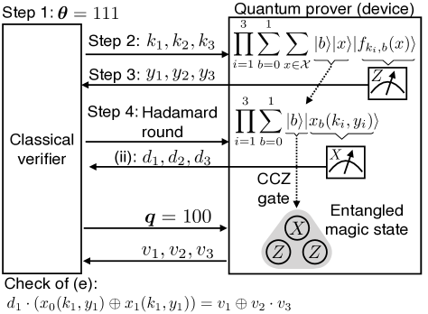
Figure 1: This figure shows the procedures for the honest device that passes step (e). If the device executes the displayed state preparation, measurements, and $CCZ$ gate operation, where the register $|f_{k_{i},b}(x)\rangle$ (register $|x_{b}(k_{i},y_{i})\rangle$) is measured in the computational (Hadamard) basis, the entangled magic state is prepared. The measurement with $\bm{q}=100$, which requests Pauli-$X$ ($Z$) measurement on the 1^st qubit ($2^{{\rm nd}}$ and 3^rd qubits), corresponds to measuring the generalized stabilizer of the entangled magic state. Therefore, the outcomes $v_{1},v_{2},v_{3}$ of this honest device pass the check at step (e).

Below, we describe Protocol 1, which consists of a three-round interaction between the classical verifier and the computationally bounded quantum prover (see Fig. 1). The target state of our C-ST protocol is the $Z$-rotated entangled magic state, which is defined for $s_{1},s_{2},s_{3}\in\{0,1\}$ by

$$|\phi_{{\rm H}}^{(s_{1},s_{2},s_{3})}\rangle:=(\sigma_{Z}^{s_{1}}\otimes\sigma_{Z}^{s_{2}}\otimes\sigma_{Z}^{s_{3}})CCZ|+\rangle^{\otimes 3}.$$ (1)

In the protocol description, $x\in_{R}\mathcal{T}$ means that the variable $x$ is chosen from set $\mathcal{T}$ uniformly at random.
Protocol 1

1. The verifier chooses bases $\bm{\theta}:=\theta_{1}\theta_{2}\theta_{3}\in_{R}\mathcal{B}:=\{000,001,010,100,111\}$. The basis choices 0 and 1 correspond to the computational and the Hadamard basis, respectively. We call the basis choice $\bm{\theta}\in\{000,001,010,100\}$ the test case and $\bm{\theta}=111$ the hypergraph case.

2. For each $i\in\{1,2,3\}$, the verifier chooses the function family $\mathcal{G}$ ($\mathcal{F}$) if $\theta_{i}=0$ ($\theta_{i}=1$). Depending on the chosen families, the verifier generates keys $k_{1},k_{2},k_{3}$ and trapdoors $t_{k_{1}},t_{k_{2}},t_{k_{3}}$. Then, the verifier sends keys $k_{1},k_{2},k_{3}$ to the prover but keeps trapdoors $t_{k_{1}},t_{k_{2}},t_{k_{3}}$ secret from the prover.

3. The verifier receives $y_{1},y_{2},y_{3}\in\mathcal{Y}$ from the prover.

4. The verifier chooses a round type from $\{{\rm preimage~{}round,~{}Hadamard~{}round}\}$ uniformly at random and sends it to the prover.
   (i) For a preimage round: the verifier receives preimages $(b_{1},x_{1};b_{2},x_{2};b_{3},x_{3})$ from the prover with $b_{i}\in\{0,1\}$ and $x_{i}\in\mathcal{X}$. The verifier rejects the prover and sets a flag $flag\leftarrow fail_{{\rm Pre}}$ unless all the preimages are correct (namely, $f_{k_{i},b_{i}}(x_{i})=y_{i}$ holds for $i=1,2,3$).
   
   (ii) For an Hadamard round: the verifier receives $d_{1},d_{2},d_{3}\in\mathcal{X}$ from the prover. Then, the verifier sends measurement bases $q_{1},q_{2},q_{3}\in_{R}\{0,1\}$ to the prover, and the prover returns measurement outcomes $v_{1},v_{2},v_{3}\in\{0,1\}$. Depending on the bases $\bm{\theta}$, the verifier executes the following checks. If the flag is set, the verifier rejects the prover.

   1. $\bm{\theta}=$000: set $flag\leftarrow fail_{{\rm Test}}$ if for $i\in_{R}\{1,2,3\}$, $q_{i}=0$ and $b(k_{i},y_{i})\neq v_{i}$ hold.

   2. $\bm{\theta}=$100: set $flag\leftarrow fail_{{\rm Test}}$ if $q_{1}=1$ and $u(k_{1},y_{1},d_{1})\oplus b(k_{2},y_{2})\cdot b(k_{3},y_{3})\neq v_{1}$ hold.

   3. $\bm{\theta}=$010: set $flag\leftarrow fail_{{\rm Test}}$ if $q_{2}=1$ and $u(k_{2},y_{2},d_{2})\oplus b(k_{1},y_{1})\cdot b(k_{3},y_{3})\neq v_{2}$ hold.

   4. $\bm{\theta}=$001: set $flag\leftarrow fail_{{\rm Test}}$ if $q_{3}=1$ and $u(k_{3},y_{3},d_{3})\oplus b(k_{1},y_{1})\cdot b(k_{2},y_{2})\neq v_{3}$ hold.

   5. $\bm{\theta}=$111: set $flag\leftarrow fail_{{\rm Hyper}}$ if one of the following holds:
      $\bm{q}=100~{}{\rm and}~{}u(k_{1},y_{1},d_{1})\neq v_{1}\oplus v_{2}\cdot v_{3},$
      $\bm{q}=010~{}{\rm and}~{}u(k_{2},y_{2},d_{2})\neq v_{2}\oplus v_{1}\cdot v_{3},$
      $\bm{q}=001~{}{\rm and}~{}u(k_{3},y_{3},d_{3})\neq v_{3}\oplus v_{1}\cdot v_{2}$
      with $\bm{q}:=q_{1}q_{2}q_{3}$.

Completeness. We show in Theorem 1 that Protocol 1 satisfies the aforementioned completeness.

Theorem 1

There exists a computationally bounded quantum prover that is accepted in Protocol 1 with probability $1-{\rm negl}(\lambda)$. Here, ${\rm negl}(\lambda)$ is a negligible function in the security parameter $\lambda$, namely a function that decays faster than any inverse polynomial in $\lambda$.

The device is accepted in Protocol 1 if all the checks in the preimage and Hadamard rounds are passed, whose details are given in Sec. III of the Supplemental Material supple . Here, we particularly explain the procedures for the honest device that can pass step (e). Since step (e) corresponds to the check of the generalized stabilizers, the honest device passes this check if it generates the entangled magic state. Figure 1 shows how to generate this state. After returning $d_{1},d_{2},d_{3}$, the state of the honest device is close to a tensor product of three Pauli-$X$ basis eigenstates due to the claw-free property of function family $\mathcal{F}$, and hence applying the $CCZ$ gate to this state results in the entangled magic state up to Pauli-$Z$ operators.

Soundness. We next show in Theorem 2 that Protocol 1 satisfies the aforementioned soundness. For the purpose of self-testing, we are interested in the last round of the interaction [step 4 (ii)] when $\bm{\theta}=111$. Here, the verifier sends the measurement bases $\bm{q}\in\{0,1\}^{3}$ to the device and receives the outcomes $\bm{v}:=v_{1}v_{2}v_{3}\in\{0,1\}^{3}$. We can model the behavior of the device in step 4 (ii) when $\bm{\theta}=111$ by the unnormalized state $\sigma^{(s_{1},s_{2},s_{3})}$ on the device’s Hilbert space $\mathcal{H}$ with $s_{1},s_{2},s_{3}\in\{0,1\}$ and projective measurements $\{P_{\bm{q}}^{(\bm{v})}\}_{\bm{v}}$ on this state that output $\bm{v}$ given inputs $\bm{q}$ to the device. Here, $s_{i}$ is determined by bit $u(k_{i},y_{i},d_{i})$ for $i\in\{1,2,3\}$.

The goal of Protocol 1 is to ensure that the state $\sigma^{\prime(s_{1},s_{2},s_{3})}:=\sigma^{(s_{1},s_{2},s_{3})}/{\rm tr}[\sigma^{(s_{1},s_{2},s_{3})}]$ is close to the entangled magic state defined in Eq. (1), which is the target state to certify, and measurements $P_{\bm{q}}^{(\bm{v})}$ are specific tensor products of Pauli measurements, up to an isometry and a small error. This error is quantified by the probabilities that the verifier rejects the prover, namely the verifier sets a $flag$ to $fail_{{\rm Pre}}$, $fail_{{\rm Test}}$ or $fail_{{\rm Hyper}}$. We now present the soundness as follows, where $p_{{\rm a}}:={\rm Pr}\{flag\leftarrow fail_{{\rm a}}\}$ with ${\rm a}\in\{{\rm Pre,}{\rm Test},{\rm Hyper}\}$, $||\cdot||_{1}$ being the trace norm, and $P[|\cdot\rangle]:=|\cdot\rangle\langle\cdot|$.

Theorem 2

Consider a device that is rejected by the verifier with probabilities $p_{{\rm Pre}}$, $p_{{\rm Test}}$ and $p_{{\rm Hyper}}$, and make the LWE assumption. Let $|\phi_{{\rm H}}^{(s_{1},s_{2},s_{3})}\rangle$ be the target entangled magic state to certify with $s_{1},s_{2},s_{3}\in\{0,1\}$, state $\sigma^{\prime(s_{1},s_{2},s_{3})}$ defined above, $\lambda$ the security parameter, $\mathcal{H}$ the device’s Hilbert space, and $\mathcal{H}^{\prime}$ some Hilbert space. Then, there exists an isometry $V:\mathcal{H}\to\mathbb{C}^{8}\otimes\mathcal{H}^{\prime}$, states $\zeta^{(s_{1},s_{2},s_{3})}_{\mathcal{H}^{\prime}}$ on $\mathcal{H}^{\prime}$, and a constant $r>0$ such that in the case of $\bm{\theta}=111$ (hypergraph case),

$$\Big{|}\Big{|}V\sigma^{\prime(s_{1},s_{2},s_{3})}V^{\dagger}-|\phi_{{\rm H}}^{(s_{1},s_{2},s_{3})}\rangle\langle\phi_{{\rm H}}^{(s_{1},s_{2},s_{3})}|\otimes\zeta^{(s_{1},s_{2},s_{3})}_{\mathcal{H}^{\prime}}\Big{|}\Big{|}^{2}_{1}$$

$$\leq O(p_{{\rm Pre}}^{r}+p_{{\rm Test}}^{r}+p_{{\rm Hyper}}^{r})+{\rm negl}(\lambda),$$ (2)

and for any $a,b,c\in\{0,1\}$ and $q_{1},q_{2},q_{3}\in\{0,1\}$,

$$\Big{|}\Big{|}VP^{(abc)}_{q_{1}q_{2}q_{3}}\sigma^{\prime(s_{1},s_{2},s_{3})}P^{(abc)}_{q_{1}q_{2}q_{3}}V^{\dagger}-P[|a_{q_{1}},b_{q_{2}},c_{q_{3}}\rangle]$$

$$|\phi_{{\rm H}}^{(s_{1},s_{2},s_{3})}\rangle\langle\phi_{{\rm H}}^{(s_{1},s_{2},s_{3})}|P[|a_{q_{1}},b_{q_{2}},c_{q_{3}}\rangle]\otimes\zeta^{(s_{1},s_{2},s_{3})}_{\mathcal{H}^{\prime}}\Big{|}\Big{|}_{1}^{2}$$

$$\leq O(p_{{\rm Pre}}^{r}+p_{{\rm Test}}^{r}+p_{{\rm Hyper}}^{r})+{\rm negl}(\lambda).$$ (3)

Here, $|a_{q_{1}}\rangle$ with $a,q_{1}\in\{0,1\}$ is $|a_{q_{1}}\rangle:=|a\rangle$ if $q_{1}=0$ and $|a_{q_{1}}\rangle:=(|0\rangle+(-1)^{a}|1\rangle)/\sqrt{2}$ if $q_{1}=1$. $|b_{q_{2}}\rangle$ and $|c_{q_{3}}\rangle$ are defined analogously.

Here, Eq. (2) guarantees how precisely the prover generates the entangled magic state under the isometry $V$, and Eq. (3) how precisely it implements the specific single-qubit measurements on it according to the measurement bases $\bm{q}$. Using $V^{\dagger}V=I$, Eq. (3) also reveals that the actual probability distribution of the device $\{{\rm tr}[P^{(abc)}_{q_{1}q_{2}q_{3}}\sigma^{\prime(s_{1},s_{2},s_{3})}]\}_{a,b,c}$ is close to the ideal one obtained by measuring $|\phi_{{\rm H}}^{(s_{1},s_{2},s_{3})}\rangle$ in the Pauli-$Z$ and $X$ bases. Note that Eqs. (2) and (3) are analogous to the statements in the traditional self-testing (see e.g., McKague_2012 ; CGS17 ; selftestreview ). One notable difference from the traditional self-testing is that our isometry $V$ is allowed to be a global operation acting on the whole device’s Hilbert space $\mathcal{H}$ because we do consider the single quantum device. The proof of Theorem 2 is given in Sec. IV of the Supplemental Material supple .

Applications to the proof of quantumness. Recently, various protocols have been invented to enable the classical verifier to certify the quantumness of the device BCM+ ; mahadev ; yamakawa ; simpler ; LH21 ; Alex21 . Here, the meaning of quantumness differs depending on the protocols. For instance, the protocols BCM+ ; LH21 ; Alex21 verify whether the prover has a superposed state or not, the protocols mahadev ; yamakawa verify whether the prover can efficiently solve ${\sf BQP}$ problems, and the protocol simpler verifies that the prover can query to an oracle in superposition. Importantly, if the prover is accepted by the verifier, then the prover has quantum capability.

Our C-ST protocol given as Protocol 1 can be used for the proof of magic under the IID scenario where the device’s functionality is the same for each repetition of the protocol. To measure the magic, we focus on the max-relative entropy of magic LW20 . We adopt this measure for simplicity, but our arguments can be applied to any reasonable measure of the magic. Let $\mathfrak{D}_{\rm max}(\rho):=\log{(1+R_{g}(\rho))}$ be the max-relative entropy of magic of an $n$-qubit state $\rho$, where $R_{g}(\rho)$ is defined by the minimum of $t\geq 0$ such that $\rho\in(1+t){\rm STAB}-t\mathcal{S}$, ${\rm STAB}\subset\mathcal{S}$ is the convex hull of all $n$-qubit stabilizer states, and $\mathcal{S}$ is the set of $n$-qubit states. If $\rho$ is a stabilizer state, $R_{g}(\rho)=0$, and hence $\mathfrak{D}_{\rm max}(\rho)=0$. By contraposition, if $\mathfrak{D}_{\rm max}(\rho)>0$, state $\rho$ is a non-stabilizer state. Based on above observations, we outline the protocol for the proof of magic as follows (see Sec. V of the Supplemental Material supple ).
Protocol 2

1. The verifier and prover repeat Protocol 1 a constant number of times, and the verifier estimates the error probabilities $p_{{\rm Pre}},p_{{\rm Test}}$ and $p_{{\rm Hyper}}$ using Hoeffding’s inequality from the numbers of set flags.

2. If the estimated trace norm $T_{{\rm est}}$ [the square root of the right-hand side of Eq. (2)] is strictly less than $1/3$, then the verifier accepts the prover. Otherwise, the verifier rejects the prover.

We first show that if our protocol is passed, with a small significance level , which can be set to any value such as $10^{-10}$, the verifier can guarantee that the prover generates a state having non-zero magic up to the isometry. If state $\rho$ has no magic, we have $\langle\phi_{{\rm H}}^{(s_{1},s_{2},s_{3})}|\rho|\phi_{{\rm H}}^{(s_{1},s_{2},s_{3})}\rangle\leq 9/16$ because for any stabilizer state $|\psi\rangle$, $F:=|\langle\psi|\phi_{{\rm H}}^{(s_{1},s_{2},s_{3})}\rangle|^{2}\leq 9/16$ BBCCGH19 . Since $F\leq 9/16$ results in $||\rho-|\phi_{{\rm H}}^{(s_{1},s_{2},s_{3})}\rangle\langle\phi_{{\rm H}}^{(s_{1},s_{2},s_{3})}|||_{1}\geq 1/2$ nielsen10 , Hoeffding’s inequality with precision 1/6 implies that $T_{{\rm est}}<1/3$ holds with probability $10^{-10}$. Therefore, such a state $\rho$ is accepted with probability of at most $10^{-10}$.

On the other hand, there is a strategy that passes this protocol with probability $1-10^{-10}$. This is because Theorem 1 states that there exists a prover’s strategy that achieves all of the error probabilities $p_{{\rm Pre}},p_{{\rm Test}}$ and $p_{{\rm Hyper}}$ being ${\rm negl}(\lambda)$, and hence from Hoeffding’s inequality, $T_{{\rm est}}\leq{\rm negl}(\lambda)+1/6<1/3$ holds except for probability $10^{-10}$.

Discussions. In this Letter, we have constructed a computational self-testing protocol for the three-qubit entangled magic state. To generalize MV20 to $n$-qubit states, there are two obstacles: (1) The verifier chooses the state bases $\theta_{1}...\theta_{n}\in_{R}\{0,1\}^{n}$ with which the prover is requested to generate the state for $n$ times. Since the target state is prepared only when all the $\theta$’s are 1, it takes exponential time on average to generate the target state. (2) The verifier checks all the patterns of measurements, namely it checks the correctness of Pauli-$Z$ and $X$ measurements for each qubit, which takes $2^{n}$ times.

Our construction would solve the first problem. We have shown for $n=3$ that the number of state bases is sufficient to be $n+2$, which means the target state is prepared on average by repeating the protocol $(n+2)$ times. We leave its rigorous analysis and the second problem as future work.

Note added. Recently, we became aware of independent related works FWZ22 and GMP22 that extend the result MV20 to self-test $n$ Bell states and $n$ BB84 states, respectively. By exploiting these results, it could be possible to extend our result to self-test $n$ tensor products of $CCZ$ magic states $CCZ|+\rangle^{\otimes 3}$.

Acknowledgments. The authors thank Tony Metger for valuable discussions on MV20 , and Go Kato, Yasuhiro Takahashi, and Tomoyuki Morimae for helpful comments. AM is supported by JST, ACT-X Grant Number JPMJAX210O, Japan. YT is supported by MEXT Quantum Leap Flagship Program (MEXT Q-LEAP) Grant Number JPMXS0118067394, JPMXS0120319794, the Grant-in-Aid for Scientific Research (A) No.JP22H00522 of JSPS, and JST [Moonshot R&D – MILLENNIA Program] Grant Number JPMJMS2061. ST is partially supported by the Grant-in-Aid for Transformative Research Areas No.JP20H05966 of JSPS, and the Grant-in-Aid for Scientific Research (A) No.JP22H00522 of JSPS.

Supplementary material: Computational self-testing for entangled magic states

I Preliminaries

I.1 Notations

We use the bold symbol $\bm{A}$ meaning $A_{1}A_{2}A_{3}$. For $i\in\{1,2,3\}$, $\bm{A}_{\bar{i}}$ denotes $\bm{A}$ except for $A_{i}$. Let the Kronecker delta be $\delta_{x,y}=0$ if $x\neq y$ and 1 if $x=y$. We denote by $|\mathcal{S}|$ the cardinality of set $\mathcal{S}$. For bit $b\in\{0,1\}$, $\bar{b}$ denotes $b\oplus 1$. We denote ${\rm wt}(x)$ by the number of 1’s in bit string $x$.

We denote $\mathcal{H}$ by an arbitrary finite-dimensional Hilbert space. The set of linear operators on Hilbert space $\mathcal{H}$ is denoted by $\mathcal{L}(\mathcal{H})$. For $A,B\in\mathcal{L}(\mathcal{H})$, we denote the commutator by $[A,B]=AB-BA$ and the anti-commutator by $\{A,B\}=AB+BA$. ${\rm Pos}(\mathcal{H})$ denotes the set of positive semidefinite operators on $\mathcal{H}$, and we denote the set of density matrices on $\mathcal{H}$ by $\mathcal{D}(\mathcal{H})=\{A\in\mathcal{L}(\mathcal{H})|A\in{\rm Pos}(\mathcal{H}),{\rm tr}[A]=1\}$. A binary observable is defined as an observable (Hermitian operator) that only has eigenvalues $\in\{1,0,-1\}$. For any binary observable $O$ and $b\in\{0,1\}$, $O^{(b)}$ denotes the projector onto the $(-1)^{b}$-eigenspace of $O$. We denote the Pauli-$Z$ and $X$ observables by $\sigma_{Z}=\sum_{b=0}^{1}(-1)^{b}|b\rangle\langle b|$ and $\sigma_{X}=\sum_{b=0}^{1}(-1)^{b}|(-)^{b}\rangle\langle(-)^{b}|$, respectively. Here, $|(-)^{b}\rangle:=(|0\rangle+(-1)^{b}|1\rangle)/\sqrt{2}$.

Let ${\rm negl}(\lambda)$ be a negligible function in the security parameter $\lambda$, namely a function that decays faster than any inverse polynomial in $\lambda$. For a countable set $\mathcal{X}$, $x\leftarrow\mathcal{X}$ denotes that $x$ is chosen uniformly at random from $\mathcal{X}$.

I.2 Cryptographic Primitives

Here, we explain the noisy trapdoor claw-free function family, which is the cryptographic primitive underlying our self-testing protocol described in Sec. II.

Definition 3 (Hellinger Distance)

For two probability densities $f_{1}$ and $f_{2}$ over finite set $\mathcal{X}$, the Hellinger distance between $f_{1}$ and $f_{2}$ is defined as

$$H^{2}(f_{1},f_{2}):=1-\sum_{x\in\mathcal{X}}\sqrt{f_{1}(x)f_{2}(x)}.$$

Definition 4 (Noisy Trapdoor Claw-free Family mahadev )

Let $\lambda\in\mathbb{N}$ be a security parameter. Let $\mathcal{X}$ and $\mathcal{Y}$ be finite sets. Let $\mathcal{K}_{\mathcal{F}}$ be a finite set of keys. A family of functions

$$\mathcal{F}:=\{f_{k,b}:\mathcal{X}\rightarrow\mathcal{D}_{\mathcal{Y}}\}_{k\in\mathcal{K}_{\mathcal{F}},b\in\{0,1\}}$$

is called a noisy trapdoor claw-free (NTCF) family if the following conditions hold:

• Efficient Function Generation: there exists an efficient probabilistic algorithm $\mathsf{GEN}_{\mathcal{F}}$ that generates a key $k\in\mathcal{K}_{\mathcal{F}}$ together with a trapdoor $t_{k}$, $(k,t_{k})\leftarrow\mathsf{GEN}_{\mathcal{F}}(1^{\lambda})$.

• Trapdoor Injective Pair: for all $k\in\mathcal{K}_{\mathcal{F}}$, the following conditions hold.

  • Trapdoor: for all $b\in\{0,1\}$ and $x\neq x^{\prime}\in\mathcal{X}$, $\mathsf{Supp}(f_{k,b}(x))\cap\mathsf{Supp}(f_{k,b}(x^{\prime}))=\emptyset$. Moreover, there exists an efficient deterministic algorithm $\mathsf{INV}_{\mathcal{F}}$ such that for all $b\in\{0,1\}$, $x\in\mathcal{X}$ and $y\in\mathsf{Supp}(f_{k,b}(x))$, $\mathsf{INV}_{\mathcal{F}}(t_{k},b,y)=x$.

  • Injective Pair: there exists a perfect matching $\mathcal{R}_{k}\subseteq\mathcal{X}\times\mathcal{X}$ such that $f_{k,0}(x_{0})=f_{k,1}(x_{1})$ if and only if $(x_{0},x_{1})\in\mathcal{R}_{k}$.

• Efficient Range Superposition: for all $k\in\mathcal{K}_{\mathcal{F}}$ and $b\in\{0,1\}$ there exists a function $f_{k,b}^{\prime}:\mathcal{X}\rightarrow\mathcal{D}_{\mathcal{Y}}$ such that

  • For all $(x_{0},x_{1})\in\mathcal{R}_{k}$ and $y\in\mathsf{Supp}(f_{k,b}^{\prime}(x_{b}))$, $\mathsf{INV}_{\mathcal{F}}(t_{k},b,y)=x_{b}$ and $\mathsf{INV}_{\mathcal{F}}(t_{k},b\oplus 1,y)=x_{b\oplus 1}$.

  • There exists an efficient deterministic procedure $\mathsf{CHK}_{\mathcal{F}}$ that on input $k$, $b\in\{0,1\}$, $x\in\mathcal{X}$, and $y\in\mathcal{Y}$, returns $1$ if $y\in\mathsf{Supp}(f_{k,b}^{\prime}(x))$ and $0$ otherwise. Note that $\mathsf{CHK}_{\mathcal{F}}$ is not provided the trapdoor $t_{k}$.

  • For every $k\in\mathcal{K}_{\mathcal{F}}$ and $b\in\{0,1\}$,

    $$\mathrm{E}_{x\leftarrow\mathcal{X}}[H^{2}(f_{k,b}(x),f^{\prime}_{k,b}(x))]={\rm negl}(\lambda)$$

    for some negligible function ${\rm negl}(\cdot)$, where the expectation is taken over $x\leftarrow\mathcal{X}$. Here $H^{2}(\cdot,\cdot)$ is the Hellinger distance. Moreover, there exists an efficient procedure $\mathsf{SAMP}_{\mathcal{F}}$ that on input $k$ and $b\in\{0,1\}$, prepares the state

    $$\frac{1}{\sqrt{|\mathcal{X}|}}\sum_{x\in\mathcal{X},y\in\mathcal{Y}}\sqrt{(f^{\prime}_{k,b}(x))(y)}|x\rangle|y\rangle.$$

• Adaptive Hardcore Bit: for all $k\in\mathcal{K}_{\mathcal{F}}$ the following conditions hold for some integer $w$ that is a polynomially bounded function in $\lambda$.

  • For all $b\in\{0,1\}$ and $x\in\mathcal{X}$, there exists a set $G_{k,b,x}\subseteq\{0,1\}^{w}$ such that ${\rm Pr}_{d\leftarrow\{0,1\}^{w}}\{d\notin G_{k,b,x}\}$ is negligible in $\lambda$, and moreover there exists an efficient algorithm that checks for membership in $G_{k,b,x}$ given $k,b,x$ and the trapdoor $t_{k}$.

  • There is an efficiently computable injection $J:\mathcal{X}\rightarrow\{0,1\}^{w}$ such that $J$ can be inverted efficiently on its range, and such that the following holds. Let

    $$\begin{aligned} &H_{k}:=\left\{\left(b,x_{b},d,d\cdot\left(J(x_{0})\oplus J(x_{1})\right)\right)|b\in\{0,1\},(x_{0},x_{1})\in\mathcal{R}_{k},d\in G_{k,0,x_{0}}\cap G_{k,1,x_{1}}\right\},\\ &\overline{H}_{k}:=\{(b,x_{b},d,c\oplus 1)|(b,x_{b},d,c)\in H_{k}\}.\\ \end{aligned}$$

    Then for any efficient quantum algorithm $\mathcal{A}$, there exists a negligible function ${\rm negl}(\cdot)$ such that

    $$\left|{\rm Pr}_{(k,t_{k})\leftarrow\mathsf{GEN}_{\mathcal{F}}(1^{\lambda})}\{\mathcal{A}(k)\in H_{k}\}-{\rm Pr}_{(k,t_{k})\leftarrow\mathsf{GEN}_{\mathcal{F}}(1^{\lambda})}\{\mathcal{A}(k)\in\overline{H}_{k}\}\right|={\rm negl}(\lambda).$$ (4)

Definition 5 (Trapdoor Injective Function Family mahadev )

Let $\lambda\in\mathbb{N}$ be a security parameter. Let $\mathcal{X}$ and $\mathcal{Y}$ be finite sets. Let $\mathcal{K}_{\mathcal{G}}$ be a finite set of keys. A family of functions

$$\mathcal{G}:=\{f_{k,b}:\mathcal{X}\rightarrow\mathcal{D}_{\mathcal{Y}}\}_{k\in\mathcal{K}_{\mathcal{G}},b\in\{0,1\}}$$

is called a trapdoor injective function family if the following conditions hold:

• Efficient Function Generation: There exists an efficient probabilistic algorithm $\mathsf{GEN}_{\mathcal{G}}$ which generates a key $k\in\mathcal{K}_{\mathcal{G}}$ together with a trapdoor $t_{k}$, $(k,t_{k})\leftarrow\mathsf{GEN}_{\mathcal{G}}(1^{\lambda})$.

• Disjoint Trapdoor Injective Pair: For all $k\in\mathcal{K}_{\mathcal{G}}$, for all $b,b^{\prime}\in\{0,1\}$ and $x,x^{\prime}\in\mathcal{X}$, if $(b,x)\neq(b^{\prime},x^{\prime})$, $\mathsf{Supp}(f_{k,b}(x))\cap\mathsf{Supp}(f_{k,b^{\prime}}(x^{\prime}))=\emptyset$. Moreover, there exists an efficient deterministic algorithm $\mathsf{INV}_{\mathcal{G}}$ such that for all $b\in\{0,1\}$, $x\in\mathcal{X}$ and $y\in\mathsf{Supp}(f_{k,b}(x))$, $\mathsf{INV}_{\mathcal{G}}(t_{k},y)=(b,x)$.

• Efficient Range Superposition: For all $k\in\mathcal{K}_{\mathcal{G}}$ and $b\in\{0,1\}$,

  1. There exists an efficient deterministic procedure $\mathsf{CHK}_{\mathcal{G}}$ that on input $k$, $b\in\{0,1\}$, $x\in\mathcal{X}$, and $y\in\mathcal{Y}$, outputs $1$ if $y\in\mathsf{Supp}(f_{k,b}(x))$ and $0$ otherwise. Note that $\mathsf{CHK}_{\mathcal{G}}$ is not provided the trapdoor $t_{k}$.

  2. There exists an efficient procedure $\mathsf{SAMP}_{\mathcal{G}}$ that on input $k$ and $b\in\{0,1\}$ returns the state

     $$\frac{1}{\sqrt{|\mathcal{X}|}}\sum_{x\in\mathcal{X},y\in\mathcal{Y}}\sqrt{(f_{k,b}(x))(y)}|x\rangle|y\rangle.$$

Definition 6

[Injective Invariance mahadev ] A NTCF family $\mathcal{F}$ is injective invariant if there exists a trapdoor injective function family $\mathcal{G}$ such that

• The algorithm $\mathsf{CHK}_{\mathcal{F}}$ and $\mathsf{SAMP}_{\mathcal{F}}$ are the same as the algorithms $\mathsf{CHK}_{\mathcal{G}}$ and $\mathsf{SAMP}_{\mathcal{G}}$.

• For all quantum polynomial-time procedures $\mathcal{A}$, there exists a negligible function ${\rm negl}(\cdot)$ such that

  $$\left|{\rm Pr}_{(k,t_{k})\leftarrow\mathsf{GEN}_{\mathcal{F}}(1^{\lambda})}\{\mathcal{A}(k)=0\}-{\rm Pr}_{(k,t_{k})\leftarrow\mathsf{GEN}_{\mathcal{G}}(1^{\lambda})}\{\mathcal{A}(k)=0\}\right|\leq{\rm negl}(\lambda).$$

Definition 7 (Extended Trapdoor Claw-free Family mahadev )

A NTCF family $\mathcal{F}$ is an extended trapdoor claw-free family if

• $\mathcal{F}$ is injective invariant.

• For all $k\in\mathcal{K}_{\mathcal{F}}$ and $d\in\{0,1\}^{w}$, let

  $$H_{k,d}^{\prime}:=\{d\cdot(J(x_{0})\oplus J(x_{1}))|(x_{0},x_{1})\in\mathcal{R}_{k}\}.$$

  For all quantum polynomial-time algorithms $\mathcal{A}$, there exists a negligible function ${\rm negl}(\cdot)$ such that

  $$\left|{\rm Pr}_{(k,t_{k})\leftarrow\mathsf{GEN}_{\mathcal{F}}(1^{\lambda})}\{\mathcal{A}(k)\in H_{k,d}^{\prime}\}-\frac{1}{2}\right|\leq{\rm negl}(\lambda).$$

Definition 8 (Decoding maps for the ENTCF families MV20 )

We define the following maps that decode the output of an ENTCF.

• For a key $k\in\mathcal{K}_{\mathcal{G}}$ and $y\in\mathcal{Y}$, let $\hat{b}(k,y)$ be the bit such that $y$ is in the union of the supports of the distributions $f_{k,\hat{b}(k,y)}(x)$ over $x\in\mathcal{X}$. This is well-defined because the function pairs in $\mathcal{G}$ have disjoint images.

• For a key $k\in\mathcal{K}_{\mathcal{F}}$ or $\mathcal{K}_{\mathcal{G}}$, $y\in\mathcal{Y}$, and $b\in\{0,1\}$, let $\hat{x}_{b}(k,y)$ be the preimage of the function such that $y$ is in the support of the distribution $f_{k,b}(\hat{x}_{b}(k,y))$. If $y$ is not in the support, then nothing is defined for $\hat{x}_{b}(k,y)$ (so instead we define $\hat{x}_{b}(k,y):=\bot$).

• For a key $k\in\mathcal{K}_{\mathcal{F}}$, $y\in\mathcal{Y}$ and $d\in\mathcal{X}$, we define $\hat{u}(k,y,d):=d\cdot(\hat{x}_{0}(k,y)\oplus\hat{x}_{1}(k,y))$, where the preimages $\hat{x}_{0}(k,y)$ and $\hat{x}_{1}(k,y)$ can be efficiently computed by using the trapdoor information $t_{k}$.

I.3 Definitions

Throughout the paper, we adopt the following definitions based on MV20 .

Definition 9

(Distance measures)

1. For $A\in\mathcal{L}(\mathcal{H})$, the schatten-$p$ norm is defined by

   $$||A||_{p}:=[{\rm tr}(|A|^{p})]^{1/p},$$

   where $|A|:=\sqrt{A^{\dagger}A}$. Note that $||A||_{1}$ is called the trace norm, and $||A||_{\infty}$ is called the operator norm (largest singular value).

2. For $A\in\mathcal{L}(\mathcal{H})$ and $\psi\in{\rm Pos}(\mathcal{H})$, we define the state-dependent (semi) norm of $A$ with respect to $\psi$ as

   $$||A||_{\psi}:=\sqrt{{\rm tr}[A^{\dagger}A\psi]}.$$

Definition 10

(Approximate equality) We use the following symbol for describing an approximate equality.

1. For $a,b\in\mathbb{C}$, we define

   $$a\approx_{\epsilon}b\Leftrightarrow|a-b|=O(\epsilon)+{\rm negl}(\lambda).$$

2. For $A,B\in\mathcal{L}(\mathcal{H})$, we define

   $$A\approx_{\epsilon}B\Leftrightarrow||A-B||^{2}_{1}=O(\epsilon)+{\rm negl}(\lambda).$$

3. For $A,B\in\mathcal{L}(\mathcal{H})$ and $\psi\in{\rm Pos}(\mathcal{H})$, we define

   $$A\approx_{\epsilon,\psi}B\Leftrightarrow||A-B||^{2}_{\psi}=O(\epsilon)+{\rm negl}(\lambda).$$

Definition 11

(Computational indistinguishability) The two states $\psi,\psi^{\prime}\in\mathcal{D}(\mathcal{H})$ are computationally indistinguishable up to $O(\delta)$ if any efficient distinguisher, which takes as input either $\psi$ or $\psi^{\prime}$ and outputs the bit $b$, satisfies

$${\rm Pr}\{b=0|\psi\}\approx_{\delta}{\rm Pr}\{b=0|\psi^{\prime}\}.$$

We use the notation

$$\psi\overset{c}{\approx}_{\delta}\psi^{\prime}.$$

I.4 Auxiliary Lemmas

We summarize auxiliary lemmas that will be frequently used in our soundness in Sec. IV. All the lemmas in this section have been derived in MV20 . We state them here for the reader’s convenience.

Lemma 12

Let $A_{1}$ and $A_{2}$ be efficient commuting binary observables. Then $A_{1}A_{2}$ is also an efficient binary observable.

Lemma 13

1. Let $\psi\in{\rm Pos}(\mathcal{H})$, and $A,B\in\mathcal{L}(\mathcal{H})$. For $C\in\mathcal{L}(\mathcal{H})$ such that $C^{\dagger}C\leq I$ we have

   $$A\approx_{\epsilon,\psi}B\Rightarrow CA\approx_{\epsilon,\psi}CB.$$

2. Let $\psi_{i}\in{\rm Pos}(\mathcal{H})$ for $i\in\{1,...,n\}$ with constant $n$, and $A,B\in\mathcal{L}(\mathcal{H})$. Define $\psi=\sum_{i}\psi_{i}$. Then,

   $$\forall i\in\{1,...,n\}:A\approx_{\epsilon,\psi_{i}}B\Leftrightarrow A\approx_{\epsilon,\psi}B.$$

Lemma 14

Let $\psi\in{\rm Pos}(\mathcal{H})$, $\{M^{(a)}\}_{a\in\mathcal{S}}$ a projective measurement with index set $\mathcal{S}$, and $O$ denotes a binary observable

$$O=\sum_{a}(-1)^{s_{a}}M^{(a)},$$

where $s_{a}\in\{0,1\}$. Suppose there exists an $a^{\prime}\in\mathcal{S}$ such that

$${\rm tr}[M^{(a^{\prime})}\psi]\approx_{\epsilon}{\rm tr}[\psi].$$

Then,

$$O\approx_{\epsilon,\psi}(-1)^{s_{a^{\prime}}}I.$$

Lemma 15

Let $\mathcal{H}_{1}$, $\mathcal{H}_{2}$ be Hilbert spaces with $\dim(\mathcal{H}_{1})\leq\dim(\mathcal{H}_{2})$ and $V:\mathcal{H}_{1}\to\mathcal{H}_{2}$ an isometry. Let $A$ and $B$ be binary observables on $\mathcal{H}_{1}$ and $\mathcal{H}_{2}$, respectively, $\psi_{1}\in{\rm Pos}(\mathcal{H}_{1})$, $\psi_{2}\in{\rm Pos}(\mathcal{H}_{2})$, and $\epsilon\geq 0$. Then,

$${\rm tr}\left[V^{\dagger}BVA\psi_{1}\right]\approx_{\epsilon}{\rm tr}[\psi_{1}]\Rightarrow V^{\dagger}BV\approx_{\epsilon,\psi_{1}}A,$$

$${\rm tr}\left[VAV^{\dagger}B\psi_{2}\right]\approx_{\epsilon}{\rm tr}[\psi_{2}]\Rightarrow VAV^{\dagger}\approx_{\epsilon,\psi_{2}}B.$$

Lemma 16

Let $O$ be a binary observable on $\mathcal{H}$ and $\psi\in{\rm Pos}(\mathcal{H})$. Then,

$$O\approx_{\epsilon,\psi}(-1)^{b}I\Rightarrow O^{(b)}\approx_{\epsilon,\psi}I~{}{\rm and}~{}O^{(\overline{b})}\approx_{\epsilon,\psi}0.$$

Lemma 17

(Replacement lemma)

1. Let $\psi\in{\rm Pos}(\mathcal{H})$, and $A,B,C\in\mathcal{L}(\mathcal{H})$. If $A\approx_{\epsilon,\psi}B$ and $||C||_{\infty}=O(1)$, then

   $${\rm tr}[CA\psi]\approx_{\sqrt{\epsilon}}{\rm tr}[CB\psi],$$

   $${\rm tr}[AC\psi]\approx_{\sqrt{\epsilon}}{\rm tr}[BC\psi].$$

2. Let $\psi,\psi^{\prime}\in{\rm Pos}(\mathcal{H})$, and $A\in\mathcal{L}(\mathcal{H})$. If $\psi\approx_{\epsilon}\psi^{\prime}$ and $||A||_{\infty}=O(1)$, then

   $${\rm tr}[A\psi]\approx_{\sqrt{\epsilon}}{\rm tr}[A\psi^{\prime}].$$

Lemma 18

Let $A,B\in\mathcal{L}(\mathcal{H})$ be linear operators, $C\in\mathcal{L}(\mathcal{H})$ a linear operator with constant operator norm, and $\psi\in{\rm Pos}(\mathcal{H})$ with ${\rm tr}[\psi]\leq 1$. Then,

$$A\approx_{\epsilon,\psi}B\Rightarrow A\psi C\approx_{\epsilon}B\psi C~{}{\rm and~{}}C\psi A^{\dagger}\approx_{\epsilon}C\psi B^{\dagger}.$$

Lemma 19

Let $\mathcal{H}_{1}$, $\mathcal{H}_{2}$ be Hilbert spaces with $\dim(\mathcal{H}_{1})\leq\dim(\mathcal{H}_{2})$, $V:\mathcal{H}_{1}\to\mathcal{H}_{2}$ an isometry, and $A$ and $B$ binary observables on $\mathcal{H}_{1}$ and $\mathcal{H}_{2}$, respectively. Then, the following holds for any $\psi\in{\rm Pos}(\mathcal{H}_{1})$:

$$VAV^{\dagger}\approx_{\epsilon,V\psi V^{\dagger}}B\Rightarrow A\approx_{\epsilon,\psi}V^{\dagger}BV,$$

$$A\approx_{\epsilon,\psi}V^{\dagger}BV\Rightarrow VAV^{\dagger}\approx_{\sqrt{\epsilon},V\psi V^{\dagger}}B.$$

Lemma 20

Let $\mathcal{H}_{1}$, $\mathcal{H}_{2}$ be Hilbert spaces with $\dim(\mathcal{H}_{1})\leq\dim(\mathcal{H}_{2})$ and $V:\mathcal{H}_{1}\to\mathcal{H}_{2}$ an isometry. Let $A$ and $B$ be binary observables on $\mathcal{H}_{1}$ and $\mathcal{H}_{2}$, respectively, $\psi\in{\rm Pos}(\mathcal{H}_{1})$, and $\epsilon\geq 0$. Then, for any $b\in\{0,1\}$:

$$V^{\dagger}BV\approx_{\epsilon,\psi}A\Rightarrow V^{\dagger}B^{(b)}V\approx_{\epsilon,\psi}A^{(b)},$$

$$B\approx_{\epsilon,V\psi V^{\dagger}}VAV^{\dagger}\Rightarrow B^{(b)}\approx_{\epsilon,V\psi V^{\dagger}}VA^{(b)}V^{\dagger}.$$

Lemma 21

(Lifting lemma) Let $\psi$, $\psi^{\prime}\in\mathcal{D}(\mathcal{H})$ be computationally indistinguishable: $\psi\overset{c}{\approx}_{\delta}\psi^{\prime}$.

1. Let $A$, $B$ be efficient binary observables on $\mathcal{H}$. Then,

   $$A\approx_{\epsilon,\psi}B\Rightarrow A\approx_{\delta+\epsilon,\psi^{\prime}}B.$$

2. Let $A$, $B$ be efficient binary observables on $\mathcal{H}$. Then,

   $$[A,B]\approx_{\epsilon,\psi}0\Rightarrow[A,B]\approx_{\delta+\epsilon,\psi^{\prime}}0.$$

3. Let $\mathcal{H}^{\prime}$ be another Hilbert space with $\dim(\mathcal{H}^{\prime})\geq\dim(\mathcal{H})$. Also, let $\psi,\psi^{\prime}\in\mathcal{D}(\mathcal{H}^{\prime})$ such that $\psi\overset{c}{\approx}_{\delta}\psi^{\prime}$, $A$ be an efficient binary observable on $\mathcal{H}$, $B$ an efficient binary observable on $\mathcal{H}^{\prime}$, and $V:\mathcal{H}\to\mathcal{H}^{\prime}$ an efficient isometry. Then

   $$VAV^{\dagger}\approx_{\epsilon,\psi}B\Rightarrow VAV^{\dagger}\approx_{\epsilon^{1/4}+\delta,\psi^{\prime}}B.$$

II Protocol description

In this section, just for self-consistency of the Supplemental Material, we redescribe our self-testing protocol for the entangled magic state $CCZ|+\rangle^{\otimes 3}$ presented in the main text. We remark that apart from the difference of the target state to certify, our protocol design differs from the one in MV20 in the following sense. In our protocol, the verifier chooses the state basis $\bm{\theta}$ from $n+2=5$ candidates, which is linear in the number $(n)$ of qubits to certify. On the other hand, in MV20 , the verifier chooses the state basis $\bm{\theta}$ from $2^{n}$ candidates, which takes exponential time on average to generate the target state. We reduce the number of state bases by doing checks of $Z$-basis measurement only when the verifier chooses $\bm{\theta}=000$ and checks $X$-basis measurement using $\bm{\theta}$ with ${\rm wt}(\bm{\theta})=1$.
Protocol 1

1. The verifier chooses the state bases $\bm{\theta}:=\theta_{1}\theta_{2}\theta_{3}\in_{R}\mathcal{B}:=\{000,001,010,100,111\}$. The basis choices 0 and 1 correspond to the computational basis and the Hadamard basis, respectively. We call the basis choice $\bm{\theta}\in\{000,001,010,100\}$ the test case and $\bm{\theta}=111$ the hypergraph case.

2. The verifier samples public keys $k_{1},k_{2},k_{3}$ and trapdoors $t_{k_{1}},t_{k_{2}},t_{k_{3}}$ as

   $$\left\{\begin{array}[]{l}(k_{i},t_{k_{i}})\leftarrow\mathsf{GEN}_{\mathcal{G}}(1^{\lambda})~{}{\rm if}~{}\theta_{i}=0,\\ (k_{i},t_{k_{i}})\leftarrow\mathsf{GEN}_{\mathcal{F}}(1^{\lambda})~{}{\rm if}~{}\theta_{i}=1.\end{array}\right.$$ (7)

   Then, the verifier sends $k_{1},k_{2},k_{3}$ to the prover but keeps trapdoors $t_{k_{1}},t_{k_{2}},t_{k_{3}}$ secret from the prover.

3. The verifier receives $y_{1},y_{2},y_{3}\in\mathcal{Y}$ from the prover.

4. The verifier chooses the round type from $\{{\rm preimage~{}round,~{}Hadamard~{}round}\}$ uniformly at random and sends it to the prover.

   1. For a preimage round: The verifier receives $(b_{1},x_{1};b_{2},x_{2};b_{3},x_{3})$ from the prover with $b_{i}\in\{0,1\}$ and $x_{i}\in\mathcal{X}$. The verifier sets a flag $flag\leftarrow fail_{{\rm Pre}}$ except $\mathsf{CHK}(k_{i},y_{i},b_{i},x_{i})=1$ holds for all $i\in\{1,2,3\}$.

   2. For an Hadamard round: The verifier receives $d_{1},d_{2},d_{3}\in\{0,1\}^{w}$ from the prover. Then, the verifier sends the questions $q_{1},q_{2},q_{3}\in_{R}\{0,1\}$ to the prover, and the prover returns the answers $v_{1},v_{2},v_{3}\in\{0,1\}$ to the verifier. Depending on the basis choice $\bm{\theta}$, the verifier executes the following checks. If the flag is set, the verifier rejects the prover.

      Basis choice	Verifier’s check
      $\bm{\theta}$=000	Set $flag\leftarrow fail_{{\rm Test}}$ if the following is true for $i\in_{R}\{1,2.3\}$:
      	$q_{i}=0~{}~{}\wedge~{}~{}\hat{b}(k_{i},y_{i})\neq v_{i}.$
      $\bm{\theta}$=100	Set $flag\leftarrow fail_{{\rm Test}}$ if the following is true:
      	$q_{1}=1~{}~{}\wedge~{}~{}\hat{u}(k_{1},y_{1},d_{1})\oplus\hat{b}(k_{2},y_{2})\cdot\hat{b}(k_{3},y_{3})\neq v_{1}.$
      $\bm{\theta}$=010	Set $flag\leftarrow fail_{{\rm Test}}$ if the following is true:
      	$q_{2}=1~{}~{}\wedge~{}~{}\hat{u}(k_{2},y_{2},d_{2})\oplus\hat{b}(k_{1},y_{1})\cdot\hat{b}(k_{3},y_{3})\neq v_{2}.$
      $\bm{\theta}$=001	Set $flag\leftarrow fail_{{\rm Test}}$ if the following is true:
      	$q_{3}=1~{}~{}\wedge~{}~{}\hat{u}(k_{3},y_{3},d_{3})\oplus\hat{b}(k_{1},y_{1})\cdot\hat{b}(k_{2},y_{2})\neq v_{3}.$
      $\bm{\theta}$=111	Set $flag\leftarrow fail_{{\rm Hyper}}$ if one of the following is true:
      	$\bm{q}=100~{}~{}\wedge~{}~{}\hat{u}(k_{1},y_{1},d_{1})\neq v_{1}\oplus v_{2}\cdot v_{3},$
      	$\bm{q}=010~{}~{}\wedge~{}~{}\hat{u}(k_{2},y_{2},d_{2})\neq v_{2}\oplus v_{1}\cdot v_{3},$
      	$\bm{q}=001~{}~{}\wedge~{}~{}\hat{u}(k_{3},y_{3},d_{3})\neq v_{3}\oplus v_{1}\cdot v_{2}.$

III protocol completeness

In this section, we prove our Theorem 1 in the main text. Specifically, we show that there exists an honest prover’s strategy, which is accepted by the verifier with probability negligibly close to 1.

First, after receiving the keys $k_{1},k_{2},k_{3}$ from the verifier, the prover treats each key separately and prepares the following state for $i\in\{1,2,3\}$:

$$\frac{1}{\sqrt{2|\mathcal{X}|}}\sum_{b=0}^{1}\sum_{x\in\mathcal{X},y\in\mathcal{Y}}\sqrt{(f_{k_{i},b}(x))(y)}|b\rangle|x\rangle|y\rangle.$$

The preparation of this state can be efficiently done up to negligible error using the procedures from the definition of ENTCF families (definition 4.2 in mahadev ). Then, the prover measures the $y$-register and returns the outcomes $y_{1},y_{2},y_{3}\in\mathcal{Y}$ to the verifier. At this point, the post-measurement state for each $i\in\{1,2,3\}$ is written as

$$\begin{cases}|\hat{b}(k_{i},y_{i})\rangle|\hat{x}(k_{i},y_{i})\rangle&~{}~{}{\rm if~{}}k_{i}\in\mathcal{K}_{\mathcal{G}},\\ \frac{1}{\sqrt{2}}(|0\rangle|\hat{x}_{0}(k_{i},y_{i})\rangle+|1\rangle|\hat{x}_{1}(k_{i},y_{i})\rangle)&~{}~{}{\rm if~{}}k_{i}\in\mathcal{K}_{\mathcal{F}}.\end{cases}$$

Note that bit $\hat{b}(k,y)$ for $k\in\mathcal{K}_{\mathcal{G}}$ and $y\in\mathcal{Y}$, and preimage $\hat{x}_{b}(k,y)$ with $b\in\{0,1\}$, $k\in\mathcal{K}_{\mathcal{G}}\cup\mathcal{K}_{\mathcal{F}}$ and $y\in\mathcal{Y}$ are defined in Definition 8. For simplicity of notation, we define $\hat{x}(k,y):=\hat{x}_{\hat{b}(k,y)}(k,y)$. If the verifier chooses the preimage round, it is easy to figure out that the prover is accepted by the verifier with probability negligibly close to 1.

If the verifier chooses the Hadamard round, the prover measures the $x$-register in the Hadamard basis, obtains the outcomes $d_{1},d_{2},d_{3}\in\{0,1\}^{w}$ and returns these to the verifier. At this point, the prover’s state for each $i\in\{1,2,3\}$ is given by

$$\begin{cases}|\hat{b}(k_{i},y_{i})\rangle&~{}~{}{\rm if~{}}k_{i}\in\mathcal{K}_{\mathcal{G}},\\ |(-)^{\hat{u}(k_{i},y_{i},d_{i})}\rangle&~{}~{}{\rm if~{}}k_{i}\in\mathcal{K}_{\mathcal{F}}.\end{cases}$$

Here, we define $\hat{u}(k_{i},y_{i},d_{i}):=d_{i}\cdot(\hat{x}_{0}(k_{i},y_{i})\oplus\hat{x}_{1}(k_{i},y_{i}))$. Now, the prover performs the $CCZ$ gate among the three qubits and obtains

$$\begin{cases}|\hat{b}(k_{1},y_{1})\rangle|\hat{b}(k_{2},y_{2})\rangle|\hat{b}(k_{3},y_{3})\rangle~{}~{}({\rm if}~{}k_{1},k_{2},k_{3}\in\mathcal{K}_{\mathcal{G}}),\\ |(-)^{\hat{u}(k_{i},y_{i},d_{i})\oplus\hat{b}(k_{j},y_{j})\cdot\hat{b}(k_{l},y_{l})}\rangle|\hat{b}(k_{j},y_{j})\rangle|\hat{b}(k_{l},y_{l})\rangle~{}~{}({\rm if~{}}k_{i}\in\mathcal{K}_{\mathcal{F}},k_{j},k_{l}\in\mathcal{K}_{\mathcal{G}}),\\ |\phi_{{\rm H}}^{(\hat{u}(k_{1},y_{1},d_{1}),\hat{u}(k_{2},y_{2},d_{2}),\hat{u}(k_{3},y_{3},d_{3}))}\rangle~{}~{}({\rm if}~{}k_{1},k_{2},k_{3}\in\mathcal{K}_{\mathcal{F}}),\end{cases}$$ (8)

where we define $|\phi_{{\rm H}}^{(a,b,c)}\rangle:=(\sigma_{Z}^{a}\otimes\sigma_{Z}^{b}\otimes\sigma_{Z}^{c})CCZ|+\rangle^{\otimes 3}$. It is easy to find that in the first two cases of Eq. (8), the prover’s answer is accepted by the verifier. For the third case of Eq. (8), by rewriting $|\phi_{{\rm H}}^{(u_{1},u_{2},u_{3})}\rangle$ (we use the simplified notation: $u_{i}=\hat{u}(k_{i},y_{i},d_{i})$) depending on $\bm{q}$ as

$$\bm{q}=100:~{} \frac{|(-)^{u_{1}}\rangle\otimes\left[\sqrt{2}|0,(-)^{u_{3}}\rangle+(-1)^{u_{2}}|1,0\rangle\right]+(-1)^{u_{2}+u_{3}}|(-)^{u_{1}\oplus 1}\rangle\otimes|1,1\rangle}{2},$$

$$\bm{q}=010:~{} \frac{\left[\sqrt{2}|0,(-)^{u_{2}},(-)^{u_{3}}\rangle+(-1)^{u_{1}}|1,(-)^{u_{2}},0\rangle\right]+(-1)^{u_{1}+u_{3}}|1,(-)^{u_{2}\oplus 1},1\rangle}{2},$$

$$\bm{q}=001:~{} \frac{\left[\sqrt{2}|0,(-)^{u_{2}}\rangle+(-1)^{u_{1}}|1,0\rangle\right]\otimes|(-)^{u_{3}}\rangle+(-1)^{u_{1}+u_{2}}|1,1\rangle\otimes|(-)^{u_{3}\oplus 1}\rangle}{2},$$

and if the honest prover measures the qubits in the Pauli-$Z$ or $X$ basis depending on $q_{i}=0$ or $q_{i}=1$, by returning the measurement outcome as the answer $v_{i}$, it is straightforward to figure out that the prover is accepted by the verifier.   $\blacksquare$

IV protocol soundness

In this section, we provide the proof of our Theorem 2 presented in the main text.

IV.1 Modeling Devices in the Protocol

Definition 22

(Device) The behavior of an arbitrary prover can be modeled by a device $D:=(S,\Pi,M,P)$, which are specified as follows MV20 .

1. (State just after returning images $\bm{y}$) We define set of states $S:=\{\psi^{(\bm{\theta})}\}_{\bm{\theta}\in\{0,1\}^{3}}$ as

   $$\psi^{(\bm{\theta})}=\sum_{\bm{y}\in\mathcal{Y}^{3}}\psi^{(\bm{\theta})}_{\bm{y}}\otimes|\bm{y}\rangle\langle\bm{y}|_{Y}\in\mathcal{D}(\mathcal{H}_{D}\otimes\mathcal{H}_{Y}).$$ (9)

   Note that $\psi^{(\bm{\theta})}$ with $\bm{\theta}\in\mathcal{B}$ represents the state of the prover just after step 3 of Protocol 1, namely the state just after returning images $\bm{y}$ to the verifier. The state $\psi^{(\bm{\theta})}$ is implicitly averaged over the keys $(k_{1},k_{2},k_{3})$ chosen by the verifier, and all the statements we make in terms of the device $D$ hold on overage over the keys.

2. (Measurement in the preimage round) A projective measurement on systems $\mathcal{H}_{D}\otimes\mathcal{H}_{Y}$ performed in the preimage round is defined as

   $$\Pi=\left\{\Pi^{(\bm{b},\bm{x})}=\sum_{\bm{y}\in\mathcal{Y}^{3}}\Pi^{(\bm{b},\bm{x})}_{\bm{y}}\otimes|\bm{y}\rangle\langle\bm{y}|_{Y}\right\}_{\bm{b},\bm{x}}.$$

   Here, $\Pi^{(\bm{b},\bm{x})}_{\bm{y}}$ represents the projective measurement to obtain outcomes $\bm{b}\in\{0,1\}^{3}$ and $\bm{x}\in\mathcal{X}^{3}$ given $\bm{y}\in\mathcal{Y}^{3}$.

3. (Measurement and post-measurement states in the Hadamard round) A projective measurement on systems $\mathcal{H}_{D}\otimes\mathcal{H}_{Y}$ performed in the Hadamard round to obtain $\bm{d}\in\{0,1\}^{3w}$ is defined as

   $$M=\left\{M^{(\bm{d})}=\sum_{\bm{y}\in\mathcal{Y}^{3}}M^{(\bm{d})}_{\bm{y}}\otimes|\bm{y}\rangle\langle\bm{y}|_{Y}\right\}_{\bm{d}}.$$

   For any $\bm{\theta}\in\{0,1\}^{3}$, the post-measurement normalized state after measurement $M$ is written as

   $$\rho^{(\bm{\theta})}=\sum_{\bm{y}\in\mathcal{Y}^{3},\bm{d}\in\{0,1\}^{3w}}\sigma^{(\bm{\theta})}_{\bm{y},\bm{d}}\otimes|\bm{y},\bm{d}\rangle\langle\bm{y},\bm{d}|_{YR},$$ (10)

   where $\sigma^{(\bm{\theta})}_{\bm{y},\bm{d}}:=M^{(\bm{d})}_{\bm{y}}\psi^{(\bm{\theta})}_{\bm{y}}M^{(\bm{d})}_{\bm{y}}$.

4. (Measurement after receiving questions $\bm{q}$ in the Hadamard round) Given the verifier’s questions $\bm{q}\in\{0,1\}^{3}$, $P_{\bm{q}}$ denotes the projective measurement on systems $\mathcal{H}_{D}\otimes\mathcal{H}_{Y}\otimes\mathcal{H}_{R}$:

   $$P_{\bm{q}}=\left\{P_{\bm{q}}^{(\bm{v})}=\sum_{\bm{y}\in\mathcal{Y}^{3},\bm{d}\in\{0,1\}^{3w}}P_{\bm{q},\bm{y},\bm{d}}^{(\bm{v})}\otimes|\bm{y},\bm{d}\rangle\langle\bm{y},\bm{d}|_{YR}\right\}_{\bm{v}\in\{0,1\}^{3}}.$$

   By performing this measurement, the prover obtains the outcomes $\bm{v}\in\{0,1\}^{3}$ that are returned to the verifier.

Definition 23

For a device $D=(S,\Pi,M,P)$, we define a set of binary observables with projective measurement $P_{\bm{q}}$:

$$\left\{A_{i,\bm{q}}:=\sum_{\bm{v}\in\{0,1\}^{3}}(-1)^{v_{i}}P^{(\bm{v})}_{\bm{q}}\right\}_{\bm{q}\in\{0,1\}^{3}}.$$ (11)

We call $\{A_{i,\bm{q}=000}\}_{i=1}^{3}$ and $\{A_{i,\bm{q}=111}\}_{i=1}^{3}$ non-tilde observables. Any other binary observables $\{A_{i,\bm{q}}\}_{i,\bm{q}}$ are called tilde observables. Note that all the $A_{i,\bm{q}}$ act on the same Hilbert space regardless of $i$ and $\bm{q}$. The difference lies in classical post-processing of the answers $\bm{v}$, where $A_{i,\bm{q}}$ focuses only on the outcome $v_{i}$ with the other outcomes being marginalized. If two binary observables $A_{i,\bm{q}}$ and $A_{j,\bm{q}}$ have the same input $\bm{q}$, the only difference is classical post-processing of the measurement outcomes. As classical post-processing obviously commute,

$$[A_{i,\bm{q}},A_{j,\bm{q}}]=0$$ (12)

holds for any $i,j\in\{1,2,3\}$.

Definition 24

(Efficient device) A device $D$ is called efficient if state preparations for $\psi^{(\bm{\theta})}$ and measurements $\Pi,M,P_{\bm{q}}$ can be performed efficiently.

For any efficient device, from the injective invariance property (Definition 6), post-measurement states $\rho^{(\bm{\theta})}$ in Eq. (10) are shown to be computationally indistinguishable.

Lemma 25

Let $D$ be an efficient device and $\rho^{({\bm{\theta}})}$ be a post-measurement state defined in Eq. (10). Then, for any ${\bm{\theta}},{\bm{\theta}}^{\prime}\in\{0,1\}^{3}$ and quantum polynomial-time algorithm $\mathcal{D}$, there exists a negligible function ${\rm negl}(\cdot)$ such that

$$\left|{\rm Pr}\{\mathcal{D}(\rho^{({\bm{\theta}})})=0\}-{\rm Pr}\{\mathcal{D}(\rho^{({\bm{\theta}}^{\prime})})=0\}\right|\leq{\rm negl}(\lambda).$$ (13)

The same statement holds for states $\psi^{(\bm{\theta})}$ in Eq. (9) because the following proof is valid also for $\psi^{(\bm{\theta})}$.

(Proof) It suffices to show Eq. (13) for ${\bm{\theta}},{\bm{\theta}}^{\prime}\in\{0,1\}^{3}$ with ${\rm wt}({\bm{\theta}}\oplus{\bm{\theta}}^{\prime})=1$ and $\theta_{i}\neq\theta_{i}^{\prime}$. This is because once this is in hand, we can lift it to any $\bm{\theta},\bm{\theta}^{\prime}$. For instance, when $\bm{\theta}=000$ and $\bm{\theta}^{\prime}=111$, by considering the three inequalities of Eq. (13) with $(\bm{\theta},\bm{\theta}^{\prime})=(000,001),(001,011)$ and $(011,111)$ such that the weight of each pair becomes 1 and by using the triangle inequality, we obtain Eq. (13) for $\bm{\theta}=000$ and $\bm{\theta}^{\prime}=111$. To prove Eq. (13) for ${\bm{\theta}},{\bm{\theta}}^{\prime}\in\{0,1\}^{3}$ with ${\rm wt}({\bm{\theta}}\oplus{\bm{\theta}}^{\prime})=1$, we use the algorithm $\mathcal{D}$ to construct an algorithm $\mathcal{A}$ for the injective invariance of $\mathcal{F}$. Algorithm $\mathcal{A}$ is given a key $k$ of $\mathcal{F}$ or $\mathcal{G}$, sets $k_{i}:=k$ and computes the other keys $k_{j}$ from $\mathsf{GEN}_{\mathcal{G}}(1^{\lambda})$ if $\theta_{j}=0$ ($\mathsf{GEN}_{\mathcal{F}}(1^{\lambda})$ if $\theta_{j}=1$). $\mathcal{A}$ prepares a post-measurement state $\rho^{(\bm{\theta})}$ with $k_{1},k_{2}$ and $k_{3}$, which is input to $\mathcal{D}$, and $\mathcal{D}$ outputs bit $b\in\{0,1\}$. Then, we have

$$\begin{aligned} &{\rm Pr}\{\mathcal{D}(\rho^{({\bm{\theta}})})=0\}={\rm Pr}_{(k,t_{k})\leftarrow\mathsf{GEN}_{\mathcal{G}}(1^{\lambda})}\{\mathcal{A}(k)=0\},\\ &{\rm Pr}\{\mathcal{D}(\rho^{({\bm{\theta}}^{\prime})})=0\}={\rm Pr}_{(k,t_{k})\leftarrow\mathsf{GEN}_{\mathcal{F}}(1^{\lambda})}\{\mathcal{A}(k)=0\},\end{aligned}$$

and substituting these RHS to the LHS of Eq. (13), Eq. (13) holds from the injective invariance of $\mathcal{F}$.   $\blacksquare$

IV.2 Success Probabilities of a Device

If the prover’s answer is incorrect in the protocol, the verifier sets a flag. In this section, we relate the probabilities that the prover passes these checks to the states and measurements in Sec. IV.1. Note that Lemmas 26, 27 and 28 correspond to Lemmas 4.10 (i), (ii) and (iii) in MV20 , respectively.

Lemma 26

(Preimage check) Let $D=(S,\Pi,M,P)$ be a device. The probability of passing $i^{{\rm th}}$ preimage check (namely $\mathsf{CHK}(k_{i},y_{i},b_{i},x_{i})=1$) conditioned on basis choice $\bm{\theta}\in\mathcal{B}$ and the preimage round is written as

$${\rm Pr}\{{\rm Prover~{}passes~{}the}~{}i^{{\rm th}}{\rm~{}preimage~{}check}|\bm{\theta},{\rm preimage~{}round}\}$$

$$= \delta_{\theta_{i},0}\sum_{\bm{y},\bm{x}_{\bar{i}},\bm{b}_{\bar{i}}}{\rm tr}\left[\Pi^{(\hat{b}(k_{i},y_{i}),\hat{x}(k_{i},y_{i});\bm{b}_{\bar{i}},\bm{x}_{\bar{i}})}_{\bm{y}}\psi^{(\bm{\theta})}_{\bm{y}}\right]+\delta_{\theta_{i},1}\sum_{\bm{y},\bm{x}_{\bar{i}},\bm{b}_{\bar{i}},b}{\rm tr}\left[\Pi^{(b,\hat{x}_{b}(k_{i},y_{i});\bm{b}_{\bar{i}},\bm{x}_{\bar{i}})}_{\bm{y}}\psi^{(\bm{\theta})}_{\bm{y}}\right].$$ (14)

Let $p_{\min}$ denote the minimum probability of Eq. (14) over $i\in\{1,2,3\}$ and $\bm{\theta}\in\mathcal{B}$, and we define

$$\gamma_{P}(D):=1-p_{\min}.$$ (15)

Then, the upper bound on $\gamma_{P}(D)$ is obtained as

$$\gamma_{P}(D)\leq 15\cdot{\rm Pr}\{flag=fail_{{\rm Pre}}|{\rm preimage~{}round}\}.$$ (16)

Note that ${\rm Pr}\{flag=fail_{{\rm Pre}}|{\rm preimage~{}round}\}$ can be estimated through repeating the self-testing protocol.
(Proof) The way of checks in the preimage round is exactly the same as that in MV20 , and hence by the same argument done in the proof of Lemma 4.10 (i), we obtain Eq. (16). Note that 15 in Eq. (16) comes from $n\times|\mathcal{B}|=3\times 5$ with $n$ being the number of qubits to certify, where $n=2$ and $|\mathcal{B}|=4$ in MV20 .   $\blacksquare$

Lemma 27

(Test case) Let $D=(S,\Pi,M,P)$ be a device. We define

$$\gamma_{T}(D):=1-\min\left\{\sum_{\bm{v}\in\{0,1\}^{3}}{\rm tr}\left[A^{(v_{i})}_{i,\bm{q}|q_{i}=0}\sigma^{(0,v_{1};0,v_{2};0,v_{3})}\right],\sum_{\bm{v}\in\{0,1\}^{3}}{\rm tr}\left[A^{(v_{i})}_{i,\bm{q}|q_{i}=1}\sigma^{(\theta_{1},v_{1};\theta_{2},v_{2};\theta_{3},v_{3})}\right]\right\}_{i,\bm{q}_{\bar{i}}}$$ (17)

with

$$\sigma^{(0,v_{1};0,v_{2};0,v_{3})}:= \sum_{\begin{subarray}{c}\bm{y},\bm{d}:\\ \hat{b}(k_{1},y_{1})=v_{1},\hat{b}(k_{2},y_{2})=v_{2},\hat{b}(k_{3},y_{3})=v_{3}\end{subarray}}\sigma^{(000)}_{\bm{y},\bm{d}}\otimes|\bm{y},\bm{d}\rangle\langle\bm{y},\bm{d}|,$$ (18)

$$\sigma^{(\theta_{1},v_{1};\theta_{2},v_{2};\theta_{3},v_{3})}:= \sum_{\begin{subarray}{c}\bm{y},\bm{d}:\\ \hat{u}(k_{i},y_{i},d_{i})\oplus\prod_{j\neq i}\hat{b}(k_{j},y_{j})=v_{i},\hat{b}(k_{j},y_{j})=v_{j},\hat{b}(k_{l},y_{l})=v_{l}\end{subarray}}\sigma^{(\bm{\theta}~{}{\rm s.t.}~{}{\rm wt}(\bm{\theta})=1,\theta_{i}=1)}_{\bm{y},\bm{d}}\otimes|\bm{y},\bm{d}\rangle\langle\bm{y},\bm{d}|.$$ (19)

Then, the upper bound on $\gamma_{T}(D)$ is given by

$$\gamma_{T}(D)\leq 96\cdot{\rm Pr}\{flag=fail_{{\rm Test}}|{\rm Test},{\rm Hadamard~{}round}\}.$$ (20)

Note that ${\rm Pr}\{flag=fail_{{\rm Test}}|{\rm Test},{\rm Hadamard~{}round}\}$ can be estimated through repeating the self-testing protocol.
(Proof) Since the way of checks in the Hadamard round differs from that in MV20 , we provide the complete proof. The probability of obtaining $fail_{{\rm Test}}$ in the Hadamard round (HR) with the test case is written as

$${\rm Pr}\{flag=fail_{{\rm Test}}|{\rm Test},{\rm HR}\}={\rm Pr}\{\bm{\theta}=000,flag=fail_{{\rm Test}}|{\rm Test},{\rm HR}\}+{\rm Pr}\{{\rm wt}(\bm{\theta})=1,flag=fail_{{\rm Test}}|{\rm Test},{\rm HR}\}.$$ (21)

We calculate the first and second terms in turn. First, we focus on the first one:

$${\rm Pr}\{\bm{\theta}=000,flag=fail_{{\rm Test}}|{\rm Test},{\rm HR}\}={\rm Pr}\{\bm{\theta}=000|{\rm Test},{\rm HR}\}\cdot{\rm Pr}\{flag=fail_{{\rm Test}}|\bm{\theta}=000,{\rm HR}\}$$

$$= \frac{1}{12}\sum_{i=1}^{3}\sum_{b=0}^{1}\sum_{y_{i}}{\rm Pr}\{q_{i}=0,\hat{b}(k_{i},y_{i})=b,v_{i}=\bar{b}|\bm{\theta}=000,{\rm HR},i\}$$

$$= \frac{1}{8}-\frac{1}{96}\sum_{i=1}^{3}\sum_{b=0}^{1}\sum_{y_{i}}\sum_{\bm{q}_{\bar{i}}\in\{0,1\}^{2}}{\rm Pr}\{\hat{b}(k_{i},y_{i})=v_{i}=b|\bm{\theta}=000,{\rm HR},i,q_{i}=0,\bm{q}_{\bar{i}}\}.$$ (22)

Here, $\sum_{b=0}^{1}\sum_{y_{i}}{\rm Pr}\{\hat{b}(k_{i},y_{i})=v_{i}=b|\bm{\theta}=000,{\rm HR},i,q_{i}=0,\bm{q}_{\bar{i}}\}$ represents the probability that the prover’s answer $v_{i}$ is accepted by the verifier conditioned on measuring state $\rho^{(000)}$ when the input to the device is $\bm{q}$ with $q_{i}=0$. This probability can be rewritten by using the expressions of the states and measurements as

$$\sum_{b=0}^{1}{\rm tr}\left[A^{(v_{i}=b)}_{i,\bm{q}|q_{i}=0}\sum_{y_{i}:\hat{b}(k_{i},y_{i})=b}\left(|y_{i}\rangle\langle y_{i}|\rho^{(000)}|y_{i}\rangle\langle y_{i}|\right)\right]=\sum_{b=0}^{1}{\rm tr}\left(A^{(v_{i}=b)}_{i,\bm{q}|q_{i}=0}\sum_{\bm{y},\bm{d}:\hat{b}(k_{i},y_{i})=b}\sigma_{\bm{y},\bm{d}}^{(000)}\otimes|\bm{y},\bm{d}\rangle\langle\bm{y},\bm{d}|\right).$$ (23)

By using the definition of Eq. (18), Eq. (23) is rewritten as

$$\sum_{\bm{v}\in\{0,1\}^{3}}{\rm tr}(A^{(v_{i})}_{i,\bm{q}|q_{i}=0}\sigma^{(0,v_{1};0,v_{2};0,v_{3})}).$$ (24)

Next, we calculate the second term of Eq. (21):

$${\rm Pr}\{{\rm wt}(\bm{\theta})=1,flag=fail_{{\rm Test}}|{\rm Test},{\rm HR}\}=\frac{1}{4}\sum_{i=1}^{3}{\rm Pr}\{flag=fail_{{\rm Test}}|{\rm Test},{\rm HR},{\rm wt}(\bm{\theta})=1,\theta_{i}=1\}$$

$$= \frac{1}{4}\sum_{i=1}^{3}{\rm Pr}\{q_{i}=1,\hat{u}(k_{i},y_{i},d_{i})\oplus\prod_{j\neq i}\hat{b}(k_{j},y_{j})\neq v_{i}|{\rm Test},{\rm HR},{\rm wt}(\bm{\theta})=1,\theta_{i}=1\}$$

$$= \frac{1}{32}\Big{[}\sum_{i=1}^{3}\sum_{\bm{q}_{\bar{i}}}1-\sum_{i=1}^{3}\sum_{b=0}^{1}\sum_{\bm{y},d_{i}}\sum_{\bm{q}_{\bar{i}}}{\rm Pr}\{\hat{u}(k_{i},y_{i},d_{i})\oplus\prod_{j\neq i}\hat{b}(k_{j},y_{j})=v_{i}=b|{\rm Test},{\rm HR},{\rm wt}(\bm{\theta})=1,\theta_{i}=1,q_{i}=1,\bm{q}_{\bar{i}}\}\Big{]}.$$ (25)

Here, $\sum_{b=0}^{1}\sum_{\bm{y},d_{i}}{\rm Pr}\{\hat{u}(k_{i},y_{i},d_{i})\oplus\prod_{j\neq i}\hat{b}(k_{j},y_{j})=v_{i}=b|{\rm Test},{\rm HR},{\rm wt}(\bm{\theta})=1,\theta_{i}=1,q_{i}=1,\bm{q}_{\bar{i}}\}$ expresses the probability that the prover’s answer $v_{i}$ is accepted by the verifier conditioned on measuring state $\rho^{(\bm{\theta})}$ with ${\rm wt}(\bm{\theta})=1$ and $\theta_{i}=1$ when $\bm{q}$ with $q_{i}=1$ is input to the device. This probability can be written by using the expressions of the states and measurements as

$$\sum_{b=0}^{1}{\rm tr}\left(A^{(v_{i}=b)}_{i,\bm{q}|q_{i}=1}\sum_{\bm{y},\bm{d}:\hat{u}(k_{i},y_{i},d_{i})\oplus\prod_{j\neq i}\hat{b}(k_{j},y_{j})=b}\sigma_{\bm{y},\bm{d}}^{(\bm{\theta}~{}{\rm s.t.}~{}{\rm wt}(\bm{\theta})=1,\theta_{i}=1)}\otimes|\bm{y},\bm{d}\rangle\langle\bm{y},\bm{d}|\right).$$ (26)

By using the definition of Eq. (19), for $\bm{\theta}$ such that ${\rm wt}(\bm{\theta})=1$ and $\theta_{i}=1$, Eq. (26) is rewritten as

$$\sum_{\bm{v}}{\rm tr}\left(A^{(v_{i})}_{i,\bm{q}|q_{i}=1}\sigma^{(\theta_{1},v_{1};\theta_{2},v_{2};\theta_{3},v_{3})}\right).$$ (27)

By substituting Eq. (24) to Eq. (22) and Eq. (27) to Eq. (25), Eq. (21) results in

$${\rm Pr}\{flag=fail_{{\rm Test}}|{\rm Test},{\rm HR}\}=\frac{1}{2}-\frac{1}{96}\sum_{i=1}^{3}\sum_{\bm{q}_{\bar{i}}}\left({\rm tr}\left[\sum_{\bm{v}}A^{(v_{i})}_{i,\bm{q}|q_{i}=0}\sigma^{(0,v_{1};0,v_{2};0,v_{3})}\right]+3{\rm tr}\left[\sum_{\bm{v}}A^{(v_{i})}_{i,\bm{q}|q_{i}=1}\sigma^{(\theta_{1},v_{1};\theta_{2},v_{2};\theta_{3},v_{3})}\right]\right).$$

The RHS has $3\times 2^{3}$ trace terms, and its minimum term is $1-\gamma_{T}(D)$ as defined in Eq. (17). To take a lower bound on the RHS, we replace the $(3\times 2^{3}-1)$ trace terms by 1 and only one term by $1-\gamma_{T}(D)$. By doing so, we have

$${\rm Pr}\{flag=fail_{{\rm Test}}|{\rm Test},{\rm Hadamard~{}round}\} \geq\frac{1}{2}-\frac{1}{96}\left\{[(3\times 2^{2}-1)\times 1+1\times(1-\gamma_{T}(D))]+(3\times 3\times 2^{2})\times 1\right\}$$

$$=\frac{\gamma_{T}(D)}{96},$$

which results in Eq. (20).   $\blacksquare$

Lemma 28

(Hypergraph case) Let $D=(S,\Pi,M,P)$ be a device. We define

$$\gamma_{H}(D):=1-r_{\min}$$ (28)

with

$$r_{\min}:=\min\Big{\{} \sum_{\bm{s}\in\{0,1\}^{3}}{\rm tr}\left[\left(A_{1,\bm{q}=100}A_{2,\bm{q}=100}^{(0)}+A_{1,\bm{q}=100}A_{2,\bm{q}=100}^{(1)}A_{3,\bm{q}=100}\right)^{(s_{1})}\sigma^{(1,s_{1};1,s_{2};1,s_{3})}\right],$$

$$\sum_{\bm{s}\in\{0,1\}^{3}}{\rm tr}\left[\left(A_{1,\bm{q}=010}^{(0)}A_{2,\bm{q}=010}+A_{1,\bm{q}=010}^{(1)}A_{2,\bm{q}=010}A_{3,\bm{q}=010}\right)^{(s_{2})}\sigma^{(1,s_{1};1,s_{2};1,s_{3})}\right],$$

$$\sum_{\bm{s}\in\{0,1\}^{3}}{\rm tr}\left[\left(A_{1,\bm{q}=001}^{(0)}A_{3,\bm{q}=001}+A_{1,\bm{q}=001}^{(1)}A_{2,\bm{q}=001}A_{3,\bm{q}=001}\right)^{(s_{3})}\sigma^{(1,s_{1};1,s_{2};1,s_{3})}\right]\Big{\}},$$

and

$$\sigma^{(1,s_{1};1,s_{2};1,s_{3})}:=\sum_{\begin{subarray}{c}\bm{y},\bm{d}:\\ \hat{u}(k_{1},y_{1},d_{1})=s_{1},\hat{u}(k_{2},y_{2},d_{2})=s_{2},\hat{u}(k_{3},y_{3},d_{3})=s_{3}\end{subarray}}\sigma^{(111)}_{\bm{y},\bm{d}}\otimes|\bm{y},\bm{d}\rangle\langle\bm{y},\bm{d}|.$$ (29)

Then, the upper bound on $\gamma_{H}(D)$ is given by

$$\gamma_{H}(D)\leq 8\cdot{\rm Pr}\{flag=fail_{{\rm Hyper}}|\bm{\theta}=111,{\rm Hadamard~{}round}\}.$$ (30)

Note that ${\rm Pr}\{flag=fail_{{\rm Hyper}}|\bm{\theta}=111,{\rm Hadamard~{}round}\}$ can be estimated through repeating the protocol.
(Proof) The probability of obtaining $fail_{{\rm Hyper}}$ conditioned on choosing the hypergraph case ($\bm{\theta}=111$) and the Hadamard round (HR) is calculated as

$${\rm Pr}\{flag=fail_{{\rm Hyper}}|\bm{\theta}=111,{\rm HR}\}=\sum_{i=1}^{3}{\rm Pr}\{q_{i}=1,\bm{q}_{\bar{i}}=00,\hat{u}(k_{i},y_{i},d_{i})\neq v_{i}\oplus\prod_{j\neq i}v_{j}|\bm{\theta}=111,{\rm HR}\}$$

$$= \frac{1}{8}\sum_{b=0}^{1}\sum_{i=1}^{3}\sum_{y_{i},d_{i}}{\rm Pr}\{\hat{u}(k_{i},y_{i},d_{i})=b,v_{i}\oplus\prod_{j\neq i}v_{j}=\bar{b}|\bm{\theta}=111,{\rm HR},q_{i}=1,\bm{q}_{\bar{i}}=00\}$$

$$= \frac{3}{8}-\frac{1}{8}\sum_{b=0}^{1}\sum_{i=1}^{3}\sum_{y_{i},d_{i}}{\rm Pr}\{\hat{u}(k_{i},y_{i},d_{i})=v_{i}\oplus\prod_{j\neq i}v_{j}=b|\bm{\theta}=111,{\rm HR},q_{i}=1,\bm{q}_{\bar{i}}=00\}.$$ (31)

Here, in the case of $i=1$,

$$\sum_{b=0}^{1}\sum_{y_{i},d_{i}}{\rm Pr}\{\hat{u}(k_{i},y_{i},d_{i})=v_{i}\oplus\prod_{j\neq i}v_{j}=b|\bm{\theta}=111,{\rm HR},q_{i}=1,\bm{q}_{\bar{i}}=00\}$$ (32)

represents the probability that the prover’s answer $v_{1}\oplus v_{2}\cdot v_{3}$ is accepted by the verifier conditioned on measuring state $\rho^{(111)}$ when $\bm{q}=100$ is input to the device. This probability can be rewritten by using the expressions of the states and measurements as

$$\sum_{b=0}^{1}{\rm tr}\left[(A_{1,\bm{q}=100}A_{2,\bm{q}=100}^{(0)}+A_{1,\bm{q}=100}A_{2,\bm{q}=100}^{(1)}A_{3,\bm{q}=100})^{(b)}\sum_{\begin{subarray}{c}y_{1},d_{1}:\\ \hat{u}(k_{1},y_{1},d_{1})=b\end{subarray}}\left(|y_{1},d_{1}\rangle\langle y_{1},d_{1}|\rho^{(111)}|y_{1},d_{1}\rangle\langle y_{1},d_{1}|\right)\right]$$

$$= \sum_{\bm{s}\in\{0,1\}^{3}}{\rm tr}\left[(A_{1,\bm{q}=100}A_{2,\bm{q}=100}^{(0)}+A_{1,\bm{q}=100}A_{2,\bm{q}=100}^{(1)}A_{3,\bm{q}=100})^{(s_{1})}\sigma^{(1,s_{1};1,s_{2};1,s_{3})}\right],$$ (33)

where $\sigma^{(1,s_{1};1,s_{2};1,s_{3})}$ is defined in Eq. (29). Also, we obtain analogous expressions for $i=2,3$ in Eq. (32). By substituting these three expressions to Eq. (31) and using the definition in Eq. (28), we obtain its lower bound as ${\rm Pr}\{flag=fail_{{\rm Hyper}}|\bm{\theta}=111,{\rm HR}\}\geq 3/8-(2+r_{\min})/8=\gamma_{H}(D)/8$, which results in Eq. (30).   $\blacksquare$

Next, we introduce a perfect device, whose $\gamma_{P}(D)$ in Eq. (15) is negligible. This means that the perfect device can pass the preimage round of our protocol with probability $1-{\rm negl}(\lambda)$.

Definition 29

(Perfect device). We call a device $D=(S,\Pi,M,P)$ perfect if $\gamma_{P}(D)={\rm negl}(\lambda).$

The following lemma claims that for any efficient device $D$, we can efficiently construct another efficient perfect device $D^{\prime}$, which uses the same measurements as $D$, and whose initial state is close to the one of $D$. Lemma 30 implies that the efficient device can be replaced with the corresponding perfect one by adding an approximation error of $O(\sqrt{\gamma_{P}(D)})$, it suffices to show the soundness proof to the efficient perfect device. We omit the proof of Lemma 30 as it is essentially the same as that of Lemma 4.13 in MV20 .

Lemma 30

Let $D=(S,\Pi,M,P)$ be an efficient device with $S=\{\psi^{(\bm{\theta})}\}_{\bm{\theta}\in\mathcal{B}}$ and $\gamma_{P}(D)<1-1/{\rm poly}(\lambda)$. Then there exists an efficient perfect device $D^{\prime}=(S^{\prime},\Pi,M,P)$, which uses the same measurements $\Pi,M,P$ and whose states $S^{\prime}=\{\psi^{\prime(\bm{\theta})}\}_{\bm{\theta}\in\mathcal{B}}$ satisfy the following for any $\bm{\theta}\in\mathcal{B}$:

$$||\psi^{(\bm{\theta})}-\psi^{\prime(\bm{\theta})}||_{1}\approx_{\sqrt{\gamma_{P}(D)}}0.$$ (34)

At the end of this section, we describe Lemma 31 and Corollary 32 that are frequently used in the rest of our soundness proof. We omit these proofs since these are essentially the same as those of Lemma 4.8 and Corollary 4.9 MV20 .

Lemma 31

Let $D=(S,\Pi,M,P)$ be a device. For any binary observable $O$, $\bm{\theta}\in\mathcal{B}$, $i\in\{1,2,3\}$ and $\epsilon\geq 0$,

$$\sum_{\bm{v}\in\{0,1\}^{3}}{\rm tr}(O^{(v_{i})}\sigma^{(\theta_{1},v_{1};\theta_{2},v_{2};\theta_{3},v_{3})})\approx_{\epsilon}1\Rightarrow\forall\bm{v}\in\{0,1\}^{3}:{\rm tr}(\sigma^{(\theta_{1},v_{1};\theta_{2},v_{2};\theta_{3},v_{3})})\approx_{\epsilon}{\rm tr}(O^{(v_{i})}\sigma^{(\theta_{1},v_{1};\theta_{2},v_{2};\theta_{3},v_{3})}),$$

where the definitions of $\sigma^{(\theta_{1},v_{1};\theta_{2},v_{2};\theta_{3},v_{3})}$ are given in Eqs. (18), (19) and (29).

Corollary 32

Let $D=(S,\Pi,M,P)$ be a device. For any binary observable $O$, $\bm{\theta}\in\mathcal{B}$, $i\in\{1,2,3\}$ and $\epsilon\geq 0$,

$$\sum_{\bm{v}\in\{0,1\}^{3}}{\rm tr}(O^{(v_{i})}\sigma^{(\theta_{1},v_{1};\theta_{2},v_{2};\theta_{3},v_{3})})\approx_{\epsilon}1\Rightarrow\forall\bm{v}\in\{0,1\}^{3}:O\approx_{\epsilon,\sigma^{(\theta_{1},v_{1};\theta_{2},v_{2};\theta_{3},v_{3})}}(-1)^{v_{i}}I,$$

where the definitions of states $\sigma^{(\theta_{1},v_{1};\theta_{2},v_{2};\theta_{3},v_{3})}$ are given in Eqs. (18), (19) and (29).

In the following Secs. IV.3 and IV.4, we only discuss the non-tilde binary observables, namely $\{A_{i,\bm{q}=000}\}_{i=1}^{3}$ and $\{A_{i,\bm{q}=111}\}_{i=1}^{3}$ in Definition 23. For simplicity, we use the notations:

$$A_{i,\bm{0}}:=A_{i,\bm{q}=000},~{}~{}A_{i,\bm{1}}:=A_{i,\bm{q}=111}.$$

IV.3 Anti-Commutation and Commutation Relations of Non-Tilde Observables

If the prover is honest, binary observables $A_{i,\bm{0}}$ and $A_{i,\bm{1}}$ are equal to the Pauli ones, which satisfy the exact commutation and anti-commutation relations. In this section, we show in Proposition 33 and Lemma 35 that these relations hold approximately for a general prover modeled by Definition IV.1.

Proposition 33

(Anti-commutation relation) For any efficient perfect device $D=(S,\Pi,M,P)$, the following approximate anti-commutation relation holds for any $i\in\{1,2,3\}$ and $\bm{\theta}\in\mathcal{B}$:

$$\{A_{i,\bm{0}},A_{i,\bm{1}}\}\approx_{\sqrt{\gamma_{T}(D)},\rho^{(\bm{\theta})}}0.$$

(Proof) Once we have the lemmas derived so far, the proof is obtained by following the same argument in Sec. 4.5 of MV20 .

Next, we turn to the commutation relation. This corresponds to Proposition 4.24 in MV20 , but due to the difference of the protocol design mentioned in Sec. II, we cannot obtain Lemma 35 just by applying the proof in MV20 . We solve this problem in Lemma 34 by proving that the statistics of the measurement outcome $v_{i}$ given $\bm{q}=000$ for $\bm{\theta}=000$ is close to that for other state basis $\bm{\theta}$.

Lemma 34

For any efficient device $D=(S,\Pi,M,P)$, the following approximate relation holds for any $\bm{\theta}\in\mathcal{B}$ with $\theta_{j}=1$ and $\theta_{i}=0$ for any $i\neq j$:

$${\rm tr}\left[\sum_{\bm{v}\in\{0,1\}^{3}}A^{(v_{i})}_{i,\bm{0}}\sigma^{(\theta_{1},v_{1};\theta_{2},v_{2};\theta_{3},v_{3})}\right]\approx_{0}{\rm tr}\left[\sum_{\bm{v}\in\{0,1\}^{3}}A^{(v_{i})}_{i,\bm{0}}\sigma^{(0,v_{1};0,v_{2};0,v_{3})}\right].$$ (35)

(Proof) The RHS [LHS] represents the probability that the prover’s answer $v_{i}$ is accepted by the verifier conditioned on measuring state $\rho^{(000)}$ [ $\rho^{(\bm{\theta})}$ (with $\theta_{j}=1$ and $\theta_{i}=0$ for any $i\neq j$)] when the input to the device is $\bm{q}=000$. We prove Eq. (35) by contradiction, namely if there exists a non-negligible difference between both sides of Eq. (35), we can construct an adversary $\mathcal{A}$ that distinguishes $\rho^{(000)}$ and $\rho^{(\bm{\theta})}$ with non-negligible advantage, which contradicts Lemma 25. The construction of $\mathcal{A}$ is as follows.

First, adversary $\mathcal{A}$ receives the $j^{{\rm th}}$ key $k_{j}$ from the verifier and samples the other keys and trapdoors from the distribution $(k_{i},t_{k_{i}})\leftarrow\mathsf{GEN}_{\mathcal{G}}(1^{\lambda})$ for $i\in\{1,2,3\}\setminus\{j\}$. Note that $\mathcal{A}$ does not know whether $k_{j}\in\mathcal{K}_{\mathcal{G}}$ or $k_{j}\in\mathcal{K}_{\mathcal{F}}$ that indicates $\theta_{j}=0$ or $\theta_{j}=1$, respectively. Then $\mathcal{A}$ prepares the state $\psi^{(\bm{\theta})}$ and measures the state to obtain $\bm{y}\in\mathcal{Y}^{3}$. After that $\mathcal{A}$ performs measurement $M$ and obtains $\bm{d}\in\{0,1\}^{3w}$. Next, by using binary observable $\{A_{i,\bm{0}}^{(v_{i})}\}_{v_{i}}$, $\mathcal{A}$ performs measurement to know whether his outcome $v_{i}$ is accepted by the verifier, that is $v_{i}=\hat{b}(k_{i},y_{i})$ holds, or not. If the outcome $v_{i}$ is accepted, $\mathcal{A}$ outputs $b=0$. The reason why $\mathcal{A}$ can judge whether $v_{i}$ is accepted or not is that $\mathcal{A}$ knows the $i^{{\rm th}}$ trapdoor. With the negation of Eq. (35), we have

$$|{\rm Pr}\{b=0|\rho^{(\bm{\theta})}\}-{\rm Pr}\{b=0|\rho^{(000)}\}|\geq\mu(\lambda).$$

This breaks the computational indistinguishability of $\rho^{(\bm{\theta})}$ stated in Lemma 25. Note that the proof of Lemma 25 reveals that this lemma also holds even when an efficient adversary $\mathcal{A}$ uses the $l^{{\rm th}}$ trapdoor, where $l$ indicates the common $\theta$ in $\bm{\theta}$ and $\bm{\theta}^{\prime}$ with ${\rm wt}(\bm{\theta}\oplus\bm{\theta}^{\prime})\in\{1,2\}$.   $\blacksquare$

Lemma 35

(Commutation relation) For any efficient device $D=(S,\Pi,M,P)$, the approximate commutation relation holds for any $\bm{\theta}\in\mathcal{B}$ and any $i,j$ of $i\neq j$:

$$[A_{i,\bm{0}},A_{j,\bm{1}}]\approx_{\gamma_{T}(D),\rho^{(\bm{\theta})}}0.$$ (36)

(Proof) From Lemma 21 (ii) and computational indistinguishability of $\rho^{(\bm{\theta})}$ stated in Lemma 25, it suffices to show Eq. (36) for a specific $\bm{\theta}$. We here fix $\bm{\theta}$ to be $\theta_{j}=1$ and $\theta_{i}=0$ for any $i\neq j$. By the definition of $\gamma_{T}(D)$ in Eq. (17), we have

$${\rm tr}\left(\sum_{\bm{v}}A^{(v_{i})}_{i,\bm{0}}\sigma^{(0,v_{1};0,v_{2};0,v_{3})}\right)\approx_{\gamma_{T}(D)}1,~{}~{}~{}{\rm tr}\left(\sum_{\bm{v}}A^{(v_{j})}_{j,\bm{1}}\sigma^{(\theta_{1},v_{1};\theta_{2},v_{2};\theta_{3},v_{3})}\right)\approx_{\gamma_{T}(D)}1.$$ (37)

Since our protocol checks the $Z$-basis measurement outcome only when $\bm{\theta}=000$, we cannot obtain the first equation of Eq. (37) for $\sigma^{(\theta_{1},v_{1};\theta_{2},v_{2};\theta_{3},v_{3})}$. To make $\sigma$’s in the above two equations to be the same, we apply Lemma 34 to the first equation of Eq. (37), which results in

$${\rm tr}\left(\sum_{\bm{v}}A^{(v_{i})}_{i,\bm{0}}\sigma^{(\theta_{1},v_{1};\theta_{2},v_{2};\theta_{3},v_{3})}\right)\approx_{\gamma_{T}(D)}1.$$ (38)

By using Corollary 32, the second equation of Eq. (37) and (38) respectively lead to $A_{j,\bm{1}}\approx_{\gamma_{T}(D),\sigma^{(\theta_{1},v_{1};\theta_{2},v_{2};\theta_{3},v_{3})}}(-1)^{v_{j}}I$ and $A_{i,\bm{0}}\approx_{\gamma_{T}(D),\sigma^{(\theta_{1},v_{1};\theta_{2},v_{2};\theta_{3},v_{3})}}(-1)^{v_{i}}I$. Finally, Lemma 13 (i) implies

$$A_{i,\bm{0}}A_{j,\bm{1}} \approx_{\gamma_{T}(D),\sigma^{(\theta_{1},v_{1};\theta_{2},v_{2};\theta_{3},v_{3})}}(-1)^{v_{j}}A_{i,\bm{0}}\approx_{\gamma_{T}(D),\sigma^{(\theta_{1},v_{1};\theta_{2},v_{2};\theta_{3},v_{3})}}(-1)^{v_{i}+v_{j}}I$$

$$\approx_{\gamma_{T}(D),\sigma^{(\theta_{1},v_{1};\theta_{2},v_{2};\theta_{3},v_{3})}}A_{j,\bm{1}}\cdot(-1)^{v_{i}}I\approx_{\gamma_{T}(D),\sigma^{(\theta_{1},v_{1};\theta_{2},v_{2};\theta_{3},v_{3})}}A_{j,\bm{1}}A_{i,\bm{0}},$$

which ends the proof.   $\blacksquare$

IV.4 Approximate Relations of Non-Tilde Observables and Pauli Observables

In this section, we introduce swap isometry. This isometry is a completely positive and trace preserving (CPTP) map that adds three-qubit Hilbert space $\mathbb{C}^{8}$ to prover’s Hilbert space $\mathcal{H}$ and swaps the three-qubit space in $\mathcal{H}$ to $\mathbb{C}^{8}$. This isometry is an extension of the one in Definition 4.27 MV20 to the three-qubit case.

Definition 36

(Swap isometry) Given a device $D=(S,\Pi,M,P)$ with Hilbert space $\mathcal{H}$, we define swap isometry $V_{S}:\mathcal{H}\to\mathbb{C}^{8}\otimes\mathcal{H}$ using non-tilde observables introduced in Eq. (11) as

$$V_{S}=\sum_{a,b,c\in\{0,1\}}|a,b,c\rangle\otimes\left[A^{c}_{3,\bm{1}}A^{(c)}_{3,\bm{0}}A^{b}_{2,\bm{1}}A^{(b)}_{2,\bm{0}}A^{a}_{1,\bm{1}}A^{(a)}_{1,\bm{0}}\right].$$ (39)

Here, superscript $a$ in $A^{a}$ indicates the exponent, and $A^{(a)}$ is the projector onto $(-1)^{a}$-eigenspace of $A$.

The goal of this section is to prove Lemmas 37, 38, 41, and 45, which state that non-tilde observables $A_{i,\bm{0}}$ and $A_{i,\bm{1}}$ are close to the Pauli observables under isometry $V_{S}$.

Lemma 37

Conjugating Pauli observables by swap isometry $V_{S}$ gives the following.

$$V_{S}^{\dagger}\sigma_{Z,1}V_{S} =A_{1,\bm{0}}$$ (40)

$$V_{S}^{\dagger}\sigma_{Z,2}V_{S} =\sum_{a=0}^{1}A^{(a)}_{1,\bm{0}}A^{a}_{1,\bm{1}}A_{2,\bm{0}}A^{a}_{1,\bm{1}}A^{(a)}_{1,\bm{0}}$$ (41)

$$V_{S}^{\dagger}\sigma_{Z,3}V_{S} =\sum_{a,b=0}^{1}A^{(a)}_{1,\bm{0}}A^{a}_{1,\bm{1}}A^{(b)}_{2,\bm{0}}A_{2,\bm{1}}^{b}A_{3,\bm{0}}A_{2,\bm{1}}^{b}A^{(b)}_{2,\bm{0}}A_{1,\bm{1}}^{a}A^{(a)}_{1,\bm{0}}$$ (42)

$$V_{S}^{\dagger}\sigma_{X,1}V_{S} =\sum_{a=0}^{1}A^{(\overline{a})}_{1,\bm{0}}A_{1,\bm{1}}A^{(a)}_{1,\bm{0}}$$ (43)

$$V_{S}^{\dagger}\sigma_{X,2}V_{S} =\sum_{a,b=0}^{1}A^{(a)}_{1,\bm{0}}A^{a}_{1,\bm{1}}A^{(b)}_{2,\bm{0}}A_{2,\bm{1}}A^{(\overline{b})}_{2,\bm{0}}A_{1,\bm{1}}^{a}A^{(a)}_{1,\bm{0}}$$ (44)

$$V_{S}^{\dagger}\sigma_{X,3}V_{S} =\sum_{a,b,c=0}^{1}A^{(a)}_{1,\bm{0}}A^{a}_{1,\bm{1}}A^{(b)}_{2,\bm{0}}A^{b}_{2,\bm{1}}A^{(\overline{c})}_{3,\bm{0}}A_{3,\bm{1}}A^{(c)}_{3,\bm{0}}A_{2,\bm{1}}^{b}A^{(b)}_{2,\bm{0}}A^{a}_{1,\bm{1}}A^{(a)}_{1,\bm{0}}$$ (45)

Here, $\sigma_{Z,i}$ and $\sigma_{X,i}$ denote $\sigma_{Z}$ and $\sigma_{X}$ acting on the $i^{{\rm th}}$ qubit, respectively.

(Proof) These can be proven by inserting Eq. (39).   $\blacksquare$

Next, we show that under isometry $V_{S}$, the binary observable $A_{1,\bm{1}}$ is approximately equal to $\sigma_{X}$.

Lemma 38

For any efficient perfect device $D=(S,\Pi,M,P)$, we have for any $\bm{\theta}\in\mathcal{B}$,

$$V_{S}^{\dagger}\sigma_{X,1}V_{S}\approx_{\sqrt{\gamma_{T}(D)},\rho^{(\bm{\theta})}}A_{1,\bm{1}}.$$ (46)

(Proof) The proof follows from that in Lemma 4.30 MV20 using Eq. (43), Proposition 33 and Lemmas 15 and 17 (i).  $\blacksquare$

From Eqs. (40) and (46), $A_{1,\bm{q}=\bm{0}}$ and $A_{1,\bm{q}=\bm{1}}$ are shown to be close to Pauli-$Z$ and $X$ observables, respectively. Using these equations, we partially characterize the prover’s states. Specifically, we show that the prover’s states can be written as product states where the first qubit is the eigenstate of either $\sigma_{Z}$ or $\sigma_{X}$ depending on $\theta_{1}\in\{0,1\}$.

Lemma 39

Let $D=(S,\Pi,M,P)$ be an efficient perfect device. For any $\bm{v}\in\{0,1\}^{3}$, there exists positive matrices $\alpha^{(0,v_{1};0,v_{2};0,v_{3})},\alpha^{(0,v_{1};0,v_{2};1,v_{3})},\alpha^{(0,v_{1};1,v_{2};0,v_{3})}$ and $\alpha^{(1,v_{1};0,v_{2};0,v_{3})}$ such that the following holds:

$$V_{S}\sigma^{(0,v_{1};0,v_{2};0,v_{3})}V_{S}^{\dagger}\approx_{\gamma_{T}(D)^{1/4}}|v_{1}\rangle\langle v_{1}|\otimes\alpha^{(0,v_{1};0,v_{2};0,v_{3})},$$ (47)

$$V_{S}\sigma^{(0,v_{1};0,v_{2};1,v_{3})}V_{S}^{\dagger}\approx_{\gamma_{T}(D)^{1/4}}|v_{1}\rangle\langle v_{1}|\otimes\alpha^{(0,v_{1};0,v_{2};1,v_{3})},$$ (48)

$$V_{S}\sigma^{(0,v_{1};1,v_{2};0,v_{3})}V_{S}^{\dagger}\approx_{\gamma_{T}(D)^{1/4}}|v_{1}\rangle\langle v_{1}|\otimes\alpha^{(0,v_{1};1,v_{2};0,v_{3})},$$ (49)

$$V_{S}\sigma^{(1,v_{1};0,v_{2};0,v_{3})}V_{S}^{\dagger}\approx_{\gamma_{T}(D)^{1/4}}|(-)^{v_{1}}\rangle\langle(-)^{v_{1}}|\otimes\alpha^{(1,v_{1};0,v_{2};0,v_{3})}.$$ (50)

There are four approximate relations since there are four states corresponding to $\bm{\theta}=000,001,010$ and 100 in the test case of our protocol. The proof is similar to Lemma 4.31 MV20 , but we give the full proof for completeness.
(Proof) We first prove Eq. (50). From Lemma 38, we have

$$A_{1,\bm{1}}\approx_{\sqrt{\gamma_{T}(D)},\rho^{(100)}}V_{S}^{\dagger}\sigma_{X,1}V_{S},$$ (51)

and applying Lemmas 13 (ii), 20 and 17 (i) in this order results in

$$\sum_{\bm{v}}{\rm tr}\left[V_{S}^{\dagger}(|(-)^{v_{1}}\rangle\langle(-)^{v_{1}}|\otimes I^{\otimes 2}_{2}\otimes I)V_{S}\sigma^{(1,v_{1};0,v_{2};0,v_{3})}\right]\approx_{\gamma_{T}(D)^{1/4}}\sum_{\bm{v}}{\rm tr}[A^{(v_{1})}_{1,\bm{1}}\sigma^{(1,v_{1};0,v_{2};0,v_{3})}].$$ (52)

From the definition of $\gamma_{T}(D)$ in Eq. (17), the RHS is approximately equal as $\approx_{\gamma_{T}(D)}1$, and hence the LHS results in

$$\sum_{\bm{v}}{\rm tr}\left[V_{S}^{\dagger}(|(-)^{v_{1}}\rangle\langle(-)^{v_{1}}|\otimes I^{\otimes 2}_{2}\otimes I)V_{S}\sigma^{(1,v_{1};0,v_{2};0,v_{3})}\right]\approx_{\gamma_{T}(D)^{1/4}}1.$$

From Lemma 16 and Corollary 32, this leads to $|(-)^{v_{1}}\rangle\langle(-)^{v_{1}}|\otimes I^{\otimes 2}_{2}\otimes I\approx_{\gamma_{T}(D)^{1/4},V_{S}\sigma^{(1,v_{1};0,v_{2};0,v_{3})}V_{S}^{\dagger}}I$. Finally, using Lemma 18 implies

$$V_{S}\sigma^{(1,v_{1};0,v_{2};0,v_{3})}V_{S}^{\dagger}\approx_{\gamma_{T}(D)^{1/4}}(|(-)^{v_{1}}\rangle\langle(-)^{v_{1}}|\otimes I^{\otimes 2}_{2}\otimes I)V_{S}\sigma^{(1,v_{1};0,v_{2};0,v_{3})}V_{S}^{\dagger}(|(-)^{v_{1}}\rangle\langle(-)^{v_{1}}|\otimes I^{\otimes 2}_{2}\otimes I).$$

By defining

$$\alpha^{(1,v_{1};0,v_{2};0,v_{3})}:=(\langle(-)^{v_{1}}|\otimes I^{\otimes 2}_{2}\otimes I)V_{S}\sigma^{(1,v_{1};0,v_{2};0,v_{3})}V_{S}^{\dagger}(|(-)^{v_{1}}\rangle\otimes I^{\otimes 2}_{2}\otimes I),$$

we obtain the desired relation of Eq. (50). The other relations Eq. (47)-(49) can be proven in the same way just by replacing Eq. (51) in the above proof with Eq. (40).   $\blacksquare$

In the following discussions, we use the simplified notation $A\approx_{R,\psi}B$ if there exists a constant $c>0$ such that $A\approx_{\gamma_{T}(D)^{c},\psi}B$.

We next show that the prover’s auxiliary states are computationally indistinguishable to the prover. We omit the proof because once Lemma 39 is in hand, the proof is exactly the same argument with that of Lemma 4.32 MV20 .

Lemma 40

Let $D=(S,\Pi,M,P)$ be an efficient perfect device. There exists a normalized state $\alpha$ such that the following holds for any $v_{1}\in\{0,1\}$:

$$\sum_{v_{2},v_{3}}V_{S}\sigma^{(0,v_{1};0,v_{2};0,v_{3})}V_{S}^{\dagger}\overset{c}{\approx}_{R}\frac{|v_{1}\rangle\langle v_{1}|}{2}\otimes\alpha,~{}~{}\sum_{v_{2},v_{3}}V_{S}\sigma^{(0,v_{1};0,v_{2};1,v_{3})}V_{S}^{\dagger}\overset{c}{\approx}_{R}\frac{|v_{1}\rangle\langle v_{1}|}{2}\otimes\alpha,$$

$$\sum_{v_{2},v_{3}}V_{S}\sigma^{(0,v_{1};1,v_{2};0,v_{3})}V_{S}^{\dagger}\overset{c}{\approx}_{R}\frac{|v_{1}\rangle\langle v_{1}|}{2}\otimes\alpha,~{}~{}\sum_{v_{2},v_{3}}V_{S}\sigma^{(1,v_{1};0,v_{2};0,v_{3})}V_{S}^{\dagger}\overset{c}{\approx}_{R}\frac{|(-)^{v_{1}}\rangle\langle(-)^{v_{1}}|}{2}\otimes\alpha.$$

So far, we have shown that the state of the first register is approximately equal to the eigenstate of the Pauli observable. Using Lemmas 25 , 35, 38 and 40 and Proposition 33, the second observables are shown to be close to the Pauli observables under isometry $V_{S}$. We omit the poof since it is essentially the same as Lemma 4.33 in MV20 .

Lemma 41

For any efficient perfect device $D=(S,\Pi,M,P)$, we have for any $\bm{\theta}\in\mathcal{B}$,

$$V_{S}^{\dagger}\sigma_{Z,2}V_{S}\approx_{R,\rho^{(\bm{\theta})}}A_{2,\bm{0}},$$ (53)

$$V_{S}^{\dagger}\sigma_{X,2}V_{S}\approx_{R,\rho^{(\bm{\theta})}}A_{2,\bm{1}}.$$ (54)

Using this result, we will characterize the state of the first and the second registers, which is an extension of Lemma 39. Specifically, we show that the prover’s states are approximately equal to the product states where the first and the second qubits are the eigenstates of the Pauli observables depending on $\theta_{1}$ and $\theta_{2}$.

Lemma 42

(Extension of Lemma 39) For any efficient and perfect device $D=(S,\Pi,M,P)$, we have for any $\bm{v}\in\{0,1\}^{3}$, there exists positive matrices $\tilde{\alpha}^{(0,v_{1};0,v_{2};0,v_{3})}$, $\tilde{\alpha}^{(0,v_{1};0,v_{2};1,v_{3})}$, $\tilde{\alpha}^{(0,v_{1};1,v_{2};0,v_{3})}$ and $\tilde{\alpha}^{(1,v_{1};0,v_{2};0,v_{3})}$ such that the following holds with $P[\cdot]:=|\cdot\rangle\langle\cdot|$.

$$V_{S}\sigma^{(0,v_{1};0,v_{2};0,v_{3})}V_{S}^{\dagger}\approx_{R}P[|v_{1},v_{2}\rangle]\otimes\tilde{\alpha}^{(0,v_{1};0,v_{2};0,v_{3})}$$ (55)

$$V_{S}\sigma^{(0,v_{1};0,v_{2};1,v_{3})}V_{S}^{\dagger}\approx_{R}P[|v_{1},v_{2}\rangle]\otimes\tilde{\alpha}^{(0,v_{1};0,v_{2};1,v_{3})}$$ (56)

$$V_{S}\sigma^{(0,v_{1};1,v_{2};0,v_{3})}V_{S}^{\dagger}\approx_{R}P[|v_{1},(-)^{v_{2}}\rangle]\otimes\tilde{\alpha}^{(0,v_{1};1,v_{2};0,v_{3})}$$ (57)

$$V_{S}\sigma^{(1,v_{1};0,v_{2};0,v_{3})}V_{S}^{\dagger}\approx_{R}P[|(-)^{v_{1}},v_{2}\rangle]\otimes\tilde{\alpha}^{(1,v_{1};0,v_{2};0,v_{3})}$$ (58)

(Proof) The proof is similar to Lemma 39 and Lemma 4.37 in MV20 , so we sketch it for Eq. (58). Applying Lemmas 41, 13 (ii), Lemma 20 and Lemma 17 (i) in this order, we have

$$\sum_{\bm{v}}{\rm tr}\left[A_{2,\bm{0}}^{(v_{2})}\sigma^{(1,v_{1};0,v_{2};0,v_{3})}\right]\approx_{R}\sum_{\bm{v}}{\rm tr}\left[V_{S}^{\dagger}(I_{2}\otimes|v_{2}\rangle\langle v_{2}|\otimes I_{2}\otimes I)V_{S}\sigma^{(1,v_{1};0,v_{2};0,v_{3})}\right].$$ (59)

From Lemma 34,

$$\sum_{\bm{v}}{\rm tr}[A_{2,\bm{0}}^{(v_{2})}\sigma^{(1,v_{1};0,v_{2};0,v_{3})}]\approx_{0}\sum_{\bm{v}}{\rm tr}[A_{2,\bm{0}}^{(v_{2})}\sigma^{(0,v_{1};0,v_{2};0,v_{3})}]$$

holds, and by the definition of $\gamma_{T}(D)$ in Eq. (17), the RHS is approximately equal to 1. This means that the RHS of Eq. (59) is also approximately equal to 1. Combining this fact, Corollary 32 and Lemma 16 results in $I_{2}\otimes|v_{2}\rangle\langle v_{2}|\otimes I_{2}\otimes I\approx_{R,V_{S}\sigma^{(1,v_{1};0,v_{2};0,v_{3})}V_{S}^{\dagger}}I$. From Lemma 39, the state in the subscript of $\approx$ is close to $|(-)^{v_{1}}\rangle\langle(-)^{v_{1}}|\otimes\alpha^{(1,v_{1};0,v_{2};0,v_{3})}$, and Lemma 17 (ii) enables us to replace the state as $I_{2}\otimes|v_{2}\rangle\langle v_{2}|\otimes I_{2}\otimes I\approx_{R,|(-)^{v_{1}}\rangle\langle(-)^{v_{1}}|\otimes\alpha^{(1,v_{1};0,v_{2};0,v_{3})}}I$. Finally, from Eq. (50) and Lemma 18, we have

$$V_{S}\sigma^{(1,v_{1};0,v_{2};0,v_{3})}V_{S}^{\dagger}\approx_{R}P[|(-)^{v_{1}},v_{2}\rangle]\otimes\tilde{\alpha}^{(1,v_{1};0,v_{2};0,v_{3})}.$$

With $\tilde{\alpha}^{(1,v_{1};0,v_{2};0,v_{3})}:=(\langle v_{2}|\otimes I)\alpha^{(1,v_{1};0,v_{2};0,v_{3})}(|v_{2}\rangle\otimes I)$, we obtain the desired relation.   $\blacksquare$

Using Lemma 42, we next show an extension of Lemma 40, which states that prover’s auxiliary states with the first and second registers are computationally indistinguishable to the prover.

Lemma 43

(Extension of Lemma 40) Let $D=(S,\Pi,M,P)$ be an efficient perfect device. There exists a normalized state $\tilde{\alpha}$ such that the following holds for any $v_{1},v_{2}\in\{0,1\}$:

$$\sum_{v_{3}}V_{S}\sigma^{(0,v_{1};0,v_{2};0,v_{3})}V_{S}^{\dagger}\overset{c}{\approx}_{R}\frac{P[|v_{1},v_{2}\rangle]}{4}\otimes\tilde{\alpha},~{}~{}\sum_{v_{3}}V_{S}\sigma^{(0,v_{1};0,v_{2};1,v_{3})}V_{S}^{\dagger}\overset{c}{\approx}_{R}\frac{P[|v_{1},v_{2}\rangle]}{4}\otimes\tilde{\alpha},$$

$$\sum_{v_{3}}V\sigma^{(0,v_{1};1,v_{2};0,v_{3})}V_{S}^{\dagger}\overset{c}{\approx}_{R}\frac{P[|v_{1},(-)^{v_{2}}\rangle]}{4}\otimes\tilde{\alpha},~{}~{}\sum_{v_{3}}V_{S}\sigma^{(1,v_{1};0,v_{2};0,v_{3})}V_{S}^{\dagger}\overset{c}{\approx}_{R}\frac{P[|(-)^{v_{1}},v_{2}\rangle]}{4}\otimes\tilde{\alpha}.$$

(Proof) By repeating exactly the same argument done in the proof of Lemma 40 and Lemma 4.39 in MV20 , we have this lemma.   $\blacksquare$

With Lemma 43 in hand, we obtain a simple corollary describing an approximate relation of state $\rho^{(\bm{\theta})}$.

Corollary 44

Let $D=(S,\Pi,M,P)$ be an efficient perfect device. There exists a normalized state $\tilde{\alpha}$ such that $\forall\bm{\theta}\in\mathcal{B}$,

$$V_{S}\rho^{(\bm{\theta})}V_{S}^{\dagger}\overset{c}{\approx}_{R}\frac{I_{2}\otimes I_{2}}{4}\otimes\tilde{\alpha}.$$ (60)

(Proof) The proof follows from the one in Corollary 4.40 MV20 . Taking the sum of the equations in Lemma 43 over $v_{1}$ and $v_{2}$ yields the the statement for $\bm{\theta}$ of the test case. We can lift up the statement for any $\bm{\theta}\in\mathcal{B}$ thanks to Lemma 25.   $\blacksquare$

So far, we have shown that the prover’s states are approximately equal to the product states where the first and the second registers are in the qubit states. Using Lemmas 35 and 41, Proposition 33 and Corollary 44, we can prove that $A_{3,\bm{0}}$ and $A_{3,\bm{1}}$ are approximately equal to the Pauli observables under isometry $V_{S}$.

Lemma 45

For any efficient perfect device $D=(S,\Pi,M,P)$, we have for any $\bm{\theta}\in\mathcal{B}$,

$$V_{S}^{\dagger}\sigma_{Z,3}V_{S}\approx_{R,\rho^{(\bm{\theta})}}A_{3,\bm{0}},$$ (61)

$$V_{S}^{\dagger}\sigma_{X,3}V_{S}\approx_{R,\rho^{(\bm{\theta})}}A_{3,\bm{1}}.$$ (62)

IV.5 Approximate Relations of Tilde Observables and Pauli Observables

In this section, we prove in Corollary 47 that the tilde observables in Eq. (11) are also close to the Pauli observables under isometry $V_{S}$. In so doing, we first prove that the tilde observables are close to the non-tilde ones.

Lemma 46

For any efficient perfect device $D=(S,\Pi,M,P)$, we have for any $\bm{\theta}\in\mathcal{B}$ and $i\in\{1,2,3\}$,

$$A_{i,\bm{q}}\approx_{\gamma_{T}(D),\rho^{(\bm{\theta})}}A_{0,\bm{0}}~{}~{}{\rm for}~{}q_{i}=0~{}{\rm and}~{}\bm{q}_{\bar{i}}\in\{0,1\}^{2}\setminus\{00\},$$

$$A_{i,\bm{q}}\approx_{\gamma_{T}(D),\rho^{(\bm{\theta})}}A_{1,\bm{1}}~{}~{}{\rm for}~{}q_{i}=1~{}{\rm and}~{}\bm{q}_{\bar{i}}\in\{0,1\}^{2}\setminus\{11\}.$$

(Proof) The proof follows from that of Lemma 4.35 in MV20 . We prove $A_{1,001}\approx_{\gamma_{T}(D),\rho^{(\bm{\theta})}}A_{1,\bm{0}}$, and the others can be proven analogously. Once we prove

$$A_{1,001}\approx_{\gamma_{T}(D),\rho^{(000)}}A_{1,\bm{0}},$$ (63)

Lemma 21 (i) implies $A_{1,001}\approx_{\gamma_{T}(D),\rho^{(\bm{\theta})}}A_{1,\bm{0}}$ for any $\bm{\theta}\in\mathcal{B}$. The conditions of Lemma 21 (i) are guaranteed by computational indistinguishability of $\rho^{(\bm{\theta})}$ in Lemma 25 and by the fact that $A_{1,001}$ and $A_{1,\bm{0}}$ are efficient binary observables. Therefore, it suffices to show Eq. (63). Moreover, thanks to Lemma 13 (ii), the proof is reduced to showing

$$A_{1,001}\approx_{\gamma_{T}(D),\sigma^{(0,v_{1};0,v_{2};0,v_{3})}}A_{1,\bm{0}}.$$ (64)

From the definition of $\gamma_{T}(D)$ in Eq. (17) and Corollary 32, we have $A_{1,001}\approx_{\gamma_{T}(D),\sigma^{(0,v_{1};0,v_{2};0,v_{3})}}(-1)^{v_{1}}I$ and $A_{1,\bm{0}}\approx_{\gamma_{T}(D),\sigma^{(0,v_{1};0,v_{2};0,v_{3})}}(-1)^{v_{1}}I$ for any $\bm{v}\in\{0,1\}^{3}$. Hence, the triangle inequality of the state dependent norm results in Eq.(64).  $\blacksquare$

Corollary 47

For any efficient perfect device $D=(S,\Pi,M,P)$, we have the following for any $\bm{\theta}\in\mathcal{B}$ and $i\in\{1,2,3\}$,

$$A_{i,\bm{q}}\approx_{R,\rho^{(\bm{\theta})}}V_{S}^{\dagger}\sigma_{Z,i}V_{S}~{}~{}{\rm for}~{}q_{i}=0~{}{\rm and}~{}\bm{q}_{\bar{i}}\in\{0,1\}^{2}\setminus\{00\},$$ (65)

$$A_{i,\bm{q}}\approx_{R,\rho^{(\bm{\theta})}}V_{S}^{\dagger}\sigma_{X,i}V_{S}~{}~{}{\rm for}~{}q_{i}=1~{}{\rm and}~{}\bm{q}_{\bar{i}}\in\{0,1\}^{2}\setminus\{11\}.$$ (66)

(Proof) We follow the proof of Corollary 4.36 in MV20 . Eqs. (65) and (66) can be proven by combining Lemma 46 with Eqs. (40), (46), (53), (54), (61) and (62).   $\blacksquare$

IV.6 Approximate Relations of Joint Observables and Products of Pauli Observables

In this section, we prove that the joint observables are close to the products of Pauli ones. Specifically, any two and three joint observables are close to the products of Pauli observables in Lemmas 51 and 52, and observables of the generalized stabilizers are close to the ideal ones in Lemma 53. These lemmas are the crux of proving our main result, Theorem 54. To derive these relations, we first prepare the extended statements of Lemmas 42 and 43 and Corollary 44 in Lemmas 48 and 49 and Corollary 50, respectively.

Lemma 48

(Extension of Lemma 42) For any efficient and perfect device $D=(S,\Pi,M,P)$, we have for any $\bm{v}\in\{0,1\}^{3}$, there exists positive matrices $\tilde{\tilde{\alpha}}^{(0,v_{1};0,v_{2};0,v_{3})}$, $\tilde{\tilde{\alpha}}^{(0,v_{1};0,v_{2};1,v_{3})}$, $\tilde{\tilde{\alpha}}^{(0,v_{1};1,v_{2};0,v_{3})}$ and $\tilde{\tilde{\alpha}}^{(1,v_{1};0,v_{2};0,v_{3})}$ such that the following holds:

$$V_{S}\sigma^{(0,v_{1};0,v_{2};0,v_{3})}V_{S}^{\dagger}\approx_{R}P[|v_{1},v_{2},v_{3}\rangle]\otimes\tilde{\tilde{\alpha}}^{(0,v_{1};0,v_{2};0,v_{3})},$$ (67)

$$V_{S}\sigma^{(0,v_{1};0,v_{2};1,v_{3})}V_{S}^{\dagger}\approx_{R}P[|v_{1},v_{2},(-)^{v_{3}}\rangle]\otimes\tilde{\tilde{\alpha}}^{(0,v_{1};0,v_{2};1,v_{3})},$$ (68)

$$V_{S}\sigma^{(0,v_{1};1,v_{2};0,v_{3})}V_{S}^{\dagger}\approx_{R}P[|v_{1},(-)^{v_{2}},v_{3}\rangle]\otimes\tilde{\tilde{\alpha}}^{(0,v_{1};1,v_{2};0,v_{3})},$$

$$V_{S}\sigma^{(1,v_{1};0,v_{2};0,v_{3})}V_{S}^{\dagger}\approx_{R}P[|(-)^{v_{1}},v_{2},v_{3}\rangle]\otimes\tilde{\tilde{\alpha}}^{(1,v_{1};0,v_{2};0,v_{3})}.$$ (69)

(Proof) The proof is similar to Lemma 42, so we sketch it for Eq. (69). Applying Lemmas 45, 13 (ii), 20 and 17 (i) in this order, we have

$$\sum_{\bm{v}}{\rm tr}\left[A^{(v_{3})}_{3,\bm{0}}\sigma^{(1,v_{1};0,v_{2};0,v_{3})}\right]\approx_{R}\sum_{\bm{v}}{\rm tr}\left[V_{S}^{\dagger}(I^{\otimes 2}_{2}\otimes|v_{3}\rangle\langle v_{3}|\otimes I)V_{S}\sigma^{(1,v_{1};0,v_{2};0,v_{3})}\right].$$ (70)

The LHS is approximately equal to 1 from Lemma 34 and the definition of $\gamma_{T}(D)$ in Eq. (17), and hence the RHS of Eq. (70) is also approximately equal to 1. Applying Corollary 32 and Lemma 16 implies $I^{\otimes 2}_{2}\otimes|v_{3}\rangle\langle v_{3}|\otimes I\approx_{R,V_{S}\sigma^{(1,v_{1};0,v_{2};0,v_{3})}V_{S}^{\dagger}}I$. From Lemma 42, $V_{S}\sigma^{(1,v_{1};0,v_{2};0,v_{3})}V_{S}^{\dagger}$ is close to $P[|(-)^{v_{1}},v_{2}\rangle]\otimes\tilde{\alpha}^{(1,v_{1};0,v_{2};0,v_{3})}$, and Lemma 17 (ii) enables us to replace these states. By combining the replaced equation, Eq. (58) and Lemma 18, we finally obtain

$$V_{S}\sigma^{(1,v_{1};0,v_{2};0,v_{3})}V_{S}^{\dagger} \approx_{R}P[|(-)^{v_{1}},v_{2},v_{3}\rangle]\otimes\tilde{\tilde{\alpha}}^{(1,v_{1};0,v_{2};0,v_{3})},$$

where we define $\tilde{\tilde{\alpha}}^{(1,v_{1};0,v_{2};0,v_{3})}:=(\langle v_{3}|\otimes I)\tilde{\alpha}^{(1,v_{1};0,v_{2};0,v_{3})}(|v_{3}\rangle\otimes I)$.   $\blacksquare$

Lemma 49

(Extension of Lemma 43) Let $D=(S,\Pi,M,P)$ be an efficient perfect device. There exists a normalized state $\tilde{\tilde{\alpha}}$ such that the following holds for any $\bm{v}\in\{0,1\}^{3}$:

$$V_{S}\sigma^{(0,v_{1};0,v_{2};0,v_{3})}V_{S}^{\dagger}\overset{c}{\approx}_{R}\frac{P[|v_{1},v_{2},v_{3}\rangle]}{8}\otimes\tilde{\tilde{\alpha}},$$ (71)

$$V_{S}\sigma^{(0,v_{1};0,v_{2};1,v_{3})}V_{S}^{\dagger}\overset{c}{\approx}_{R}\frac{P[|v_{1},v_{2},(-)^{v_{3}}\rangle]}{8}\otimes\tilde{\tilde{\alpha}},$$ (72)

$$V_{S}\sigma^{(0,v_{1};1,v_{2};0,v_{3})}V_{S}^{\dagger}\overset{c}{\approx}_{R}\frac{P[|v_{1},(-)^{v_{2}},v_{3}\rangle]}{8}\otimes\tilde{\tilde{\alpha}},$$ (73)

$$V_{S}\sigma^{(1,v_{1};0,v_{2};0,v_{3})}V_{S}^{\dagger}\overset{c}{\approx}_{R}\frac{P[|(-)^{v_{1}},v_{2},v_{3}\rangle]}{8}\otimes\tilde{\tilde{\alpha}}.$$ (74)

(Proof) The proof is similar to Lemma 43, but we spell out all the details for completeness. We first prove Eq. (73), and by using Eq. (73), we prove the rest of the equations. In so doing, we need to show that $\{\tilde{\tilde{\alpha}}^{(0,v_{1};1,v_{2};0,v_{3})}\}_{\bm{v}}$ are computationally indistinguishable. For this, we already have shown in Lemma 43 that $\{\sum_{v_{3}}\tilde{\alpha}^{(0,v_{1};1,v_{2};0,v_{3})}\}_{v_{2}}$ are computationally indistinguishable for any $v_{1}$, and by considering Lemmas 42 and 48, this implies that $\{\sum_{v_{3}}\tilde{\tilde{\alpha}}^{(0,v_{1};1,v_{2};0,v_{3})}\}_{v_{2}}$ are also computationally indistinguishable for any $v_{1}$. Therefore, the remaining task is to prove that $\{\tilde{\tilde{\alpha}}^{(0,v_{1};1,v_{2};0,v_{3})}\}_{v_{3}}$ are computationally indistinguishable for any fixed $v_{1}$ and $v_{2}$. In the following discussions, we fix $v_{1}$ and $v_{2}$. From Lemma 48, there exists a $d>0$ such that for any $v_{1},v_{2},v_{3}$,

$$\left|\left|V_{S}\sigma^{(0,v_{1};1,v_{2};0,v_{3})}V_{S}^{\dagger}-P[|v_{1},(-)^{v_{2}},v_{3}\rangle]\otimes\tilde{\tilde{\alpha}}^{(0,v_{1};1,v_{2};0,v_{3})}\right|\right|_{1}^{2}\leq\epsilon,$$ (75)

$$\left|\left|V_{S}\sigma^{(0,v_{1};0,v_{2};1,v_{3})}V_{S}^{\dagger}-P[|v_{1},v_{2},(-)^{v_{3}}\rangle]\otimes\tilde{\tilde{\alpha}}^{(0,v_{1};0,v_{2};1,v_{3})}\right|\right|_{1}^{2}\leq\epsilon$$ (76)

hold with $\epsilon:=O(\gamma_{T}(D)^{d})$. From Lemmas 42 and 48, we have that

$$\left|{\rm tr}\left[M_{0}\sum_{v_{3}^{\prime}}\tilde{\tilde{\alpha}}^{(0,v_{1};1,v_{2}=0;0,v_{3}^{\prime})}\right]-{\rm tr}\left[M_{0}\sum_{v_{3}^{\prime}}\tilde{\tilde{\alpha}}^{(0,v_{1};1,v_{2}=1;0,v_{3}^{\prime})}\right]\right|\leq 2\sqrt{\epsilon}$$ (77)

holds for any $v_{1}$ and efficient measurement $M:=\{M_{0},M_{1}\}$. For the sake of contradiction, we assume that there exists a POVM $\Lambda:=\{\Lambda_{0},\Lambda_{1}\}$ with $\Lambda_{0}+\Lambda_{1}=I$ such that

$$\left|{\rm tr}\left[\Lambda_{0}\tilde{\tilde{\alpha}}^{(0,v_{1};1,v_{2};0,v_{3}=0)}\right]-{\rm tr}\left[\Lambda_{0}\tilde{\tilde{\alpha}}^{(0,v_{1};1,v_{2};0,v_{3}=1)}\right]\right|\geq 2\mu(\lambda)+42\sqrt{\epsilon}$$ (78)

holds with a non-negligible function $\mu(\lambda)$. Under the existence of this POVM, we can construct an adversary $\mathcal{A}$ that breaks the injective invariance property in Definition 6 using an efficient measurement $\{\Gamma,I-\Gamma\}$ with

$$\Gamma:=V_{S}^{\dagger}(P[|v_{1},(-)^{v_{2}},0\rangle]\otimes\Lambda_{0})V_{S}.$$

Below, we describe the procedure of $\mathcal{A}$ that breaks the injective invariance property.

$\mathcal{A}$ is given keys $(k_{2},k_{3})$, and the task is to distinguish whether the input is $(\theta_{2},\theta_{3})=(0,1)$ or $(\theta_{2},\theta_{3})=(1,0)$. For this, $\mathcal{A}$ samples the other key and a trapdoor $(k_{1},t_{k_{1}})\leftarrow\mathsf{GEN}_{\mathcal{G}}(1^{\lambda})$, prepares the state $\psi^{(\bm{\theta})}$ by performing the same operations as the device $D$, measures the $Y$-register to obtain $\bm{y}$, followed by measuring the $R$-register to obtain $\bm{d}$. At this moment, $\mathcal{A}$ prepares the state $\rho^{(\bm{\theta})}$. Finally, $\mathcal{A}$ performs the measurement $\{\Gamma,I-\Gamma\}$. This procedure is efficient because the device $D$ and the POVM $\{\Gamma,I-\Gamma\}$ are efficient. In this procedure, we calculate the distinguishing advantage ${\rm Adv}=|{\rm tr}[\Gamma(\rho^{(010)}-\rho^{(001)})]|$ in obtaining the outcome corresponding to $\Gamma$ for the states $\rho^{(010)}$ and $\rho^{(001)}$. Once we show that this advantage is non-negligible under Eq. (78), this contradicts the injective invariance property. Hence, by taking a contraposition, we obtain the negation of Eq. (78), which is the required statement in the proof. By this discussion, we only need to prove that the advantage ${\rm Adv}$ is non-negligible from Eq. (78). First, by the definitions of $\Gamma$ and $\rho^{(\bm{\theta})}$, we have

$${\rm Adv}=\left|{\rm tr}\left[(P[|v_{1},(-)^{v_{2}},0\rangle]\otimes\Lambda_{0})\left(\sum_{\bm{v}^{\prime}}V_{S}\sigma^{(0,v_{1}^{\prime};1,v_{2}^{\prime};0,v_{3}^{\prime})}V_{S}^{\dagger}-\sum_{\bm{v}^{\prime}}V_{S}\sigma^{(0,v_{1}^{\prime};0,v_{2}^{\prime};1,v_{3}^{\prime})}V_{S}^{\dagger}\right)\right]\right|.$$ (79)

To obtain its lower bound, we exploit the relation from Hölder’s inequality:

$$\left|{\rm tr}[A(\varphi-\varphi^{\prime})]\right|\leq||A||_{\infty}\cdot||\varphi-\varphi^{\prime}||_{1}\leq\tau$$ (80)

for positive operators $\varphi$ and $\varphi^{\prime}$ satisfying $||\varphi-\varphi^{\prime}||_{1}\leq\tau$ and a linear operator $A$ satisfying $||A||_{\infty}\leq 1$. By applying Eq. (80) with Eqs. (75) and (76), Adv in Eq. (79) is lower-bounded by

$$\Big{|}\sum_{\bm{v}^{\prime}\in\{0,1\}^{3}}{\rm tr}\Big{[}(P[|v_{1},(-)^{v_{2}},0\rangle\otimes\Lambda_{0})\Big{(}P[|v_{1}^{\prime},(-)^{v_{2}^{\prime}},v_{3}^{\prime}\rangle]\otimes\tilde{\tilde{\alpha}}^{(0,v_{1}^{\prime};1,v_{2}^{\prime};0,v_{3}^{\prime})}-P[|v_{1}^{\prime},v_{2}^{\prime},(-)^{v_{3}^{\prime}}\rangle]\otimes\tilde{\tilde{\alpha}}^{(0,v_{1}^{\prime};0,v_{2}^{\prime};1,v_{3}^{\prime})}\Big{)}\Big{]}\Big{|}-16\sqrt{\epsilon}$$

$$= \left|{\rm tr}\left[\Lambda_{0}\tilde{\tilde{\alpha}}^{(0,v_{1};1,v_{2};0,0)}\right]-\frac{1}{4}\sum_{v_{2}^{\prime},v_{3}^{\prime}}{\rm tr}\left[\Lambda_{0}\tilde{\tilde{\alpha}}^{(0,v_{1};0,v_{2}^{\prime};1,v_{3}^{\prime})}\right]\right|-16\sqrt{\epsilon}$$

$$= \left|\frac{1}{2}{\rm tr}\left[\Lambda_{0}(\tilde{\tilde{\alpha}}^{(0,v_{1};1,v_{2};0,0)}-\tilde{\tilde{\alpha}}^{(0,v_{1};1,v_{2};0,1)})\right]+\frac{1}{2}\sum_{v_{3}^{\prime}}{\rm tr}[\Lambda_{0}\tilde{\tilde{\alpha}}^{(0,v_{1};1,v_{2};0,v_{3}^{\prime})}]-\frac{1}{4}\sum_{v_{2}^{\prime},v_{3}^{\prime}}{\rm tr}\left[\Lambda_{0}\tilde{\tilde{\alpha}}^{(0,v_{1};0,v_{2}^{\prime};1,v_{3}^{\prime})}\right]\right|-16\sqrt{\epsilon}$$

$$\geq \mu(\lambda)+5\sqrt{\epsilon}-\frac{1}{2}\left|\sum_{v_{3}^{\prime}}{\rm tr}[\Lambda_{0}\tilde{\tilde{\alpha}}^{(0,v_{1};1,v_{2};0,v_{3}^{\prime})}]-\frac{1}{2}\sum_{v_{2}^{\prime},v_{3}^{\prime}}{\rm tr}\left[\Lambda_{0}\tilde{\tilde{\alpha}}^{(0,v_{1};0,v_{2}^{\prime};1,v_{3}^{\prime})}\right]\right|$$

$$\geq \mu(\lambda)+5\sqrt{\epsilon}-\frac{1}{2}\left|\sum_{v_{3}^{\prime}}{\rm tr}\left[\Lambda_{0}\left(\tilde{\tilde{\alpha}}^{(0,v_{1};1,v_{2};0,v_{3}^{\prime})}-\sum_{v_{2}^{\prime}}\frac{\tilde{\tilde{\alpha}}^{(0,v_{1};1,v_{2}^{\prime};0,v_{3}^{\prime})}}{2}\right)\right]\right|-\frac{1}{4}\left|\sum_{v_{2}^{\prime},v_{3}^{\prime}}{\rm tr}\left[\Lambda_{0}\left(\tilde{\tilde{\alpha}}^{(0,v_{1};1,v_{2}^{\prime};0,v_{3}^{\prime})}-\tilde{\tilde{\alpha}}^{(0,v_{1};0,v_{2}^{\prime};1,v_{3}^{\prime})}\right)\right]\right|$$

$$\geq \mu(\lambda)+4\sqrt{\epsilon}-\frac{1}{4}\left|\sum_{v_{2}^{\prime},v_{3}^{\prime}}{\rm tr}\left[\Lambda_{0}\left(\tilde{\tilde{\alpha}}^{(0,v_{1};1,v_{2}^{\prime};0,v_{3}^{\prime})}-\tilde{\tilde{\alpha}}^{(0,v_{1};0,v_{2}^{\prime};1,v_{3}^{\prime})}\right)\right]\right|$$

$$= \mu(\lambda)+4\sqrt{\epsilon}-\frac{1}{4}\left|\sum_{v_{2}^{\prime},v_{3}^{\prime}}{\rm tr}\left[\Lambda_{0}\left\{|v_{1}\rangle\langle v_{1}|\otimes\left(P[|(-)^{v_{2}^{\prime}},v_{3}^{\prime}\rangle]\otimes\tilde{\tilde{\alpha}}^{(0,v_{1};1,v_{2}^{\prime};0,v_{3}^{\prime})}-P[|v_{2},(-)^{v_{3}^{\prime}}\rangle]\otimes\tilde{\alpha}^{(0,v_{1};0,v_{2}^{\prime};1,v_{3}^{\prime})}\right\}\right)\right]\right|,$$

where we use the triangle inequality and Eq. (78) in the first inequality, the second one follows from the triangle inequality, and the third one comes from Eq. (77). Again, by applying Eq. (80) with Eqs. (75) and (76), we obtain

$${\rm Adv}\geq \mu(\lambda)-\frac{1}{4}\left|{\rm tr}\left[\Lambda_{0}\left(\sum_{v_{2}^{\prime},v_{3}^{\prime}}V_{S}\sigma^{(0,v_{1};1,v_{2}^{\prime};0,v_{3}^{\prime})}V_{S}^{\dagger}-\sum_{v_{2}^{\prime},v_{3}^{\prime}}V_{S}\sigma^{(0,v_{1};0,v_{2}^{\prime};1,v_{3}^{\prime})}V_{S}^{\dagger}\right)\right]\right|.$$

Finally, by Eq.  (19) and $\rho^{(\bm{\theta})}=\sum_{\bm{v}}\sigma^{(\theta_{1},v_{1};\theta_{2},v_{2};\theta_{3},v_{3})}$, the RHS is equal to $\mu(\lambda)-\frac{1}{4}\left|{\rm tr}\left[W\left(\rho^{(010)}-\rho^{(001)}\right)\right]\right|$ with $W:=\sum_{y_{1}:\hat{b}(k_{1},y_{1})=v_{1}}|y_{1}\rangle\langle y_{1}|V_{S}^{\dagger}\Lambda_{0}V_{S}\sum_{y_{1}:\hat{b}(k_{1},y_{1})=v_{1}}|y_{1}\rangle\langle y_{1}|.$ The measurement $\{W,I-W\}$ is efficient since $\mathcal{A}$ has the information of the trapdoor $t_{k_{1}}$ and computing $\hat{b}(k_{1},y_{1})$ is efficient. Hence, the computational indistinguishability in Lemma 25 reveals that the second term is ${\rm negl}(\lambda)$, namely

$${\rm Adv}=|{\rm tr}[\Gamma(\rho^{(010)}-\rho^{(001)})]|\geq\mu(\lambda)-{\rm negl}(\lambda).$$

This contradicts Lemma 25 and completes the proof of Eq. (73).

Next, we prove Eqs. (71), (72) and (74) using Eq. (73). First, from Eq. (73) and using the fact that $\rho^{(\bm{\theta})}$ are computationally indistinguishable from Lemma 25 and isometry $V_{S}$ is efficient, we have

$$V_{S}\rho^{(\bm{\theta})}V_{S}^{\dagger}=\sum_{\bm{v}}V_{S}\sigma^{(\theta_{1},v_{1};\theta_{2},v_{2};\theta_{3},v_{3})}V_{S}^{\dagger}\overset{c}{\approx}_{R}\frac{I_{2}^{\otimes 3}}{8}\otimes\tilde{\tilde{\alpha}}$$ (81)

for $\bm{\theta}\in\{000,001,010,100\}$. Combining Eq. (81) with Eqs. (67), (68) and (69), we respectively obtain

$$\sum_{\bm{v}}P[|v_{1},v_{2},v_{3}\rangle]\otimes\tilde{\tilde{\alpha}}^{(0,v_{1};0,v_{2};0,v_{3})}\overset{c}{\approx}_{R}I_{2}^{\otimes 3}\otimes\frac{\tilde{\tilde{\alpha}}}{8},$$

$$\sum_{\bm{v}}P[|v_{1},v_{2},(-)^{v_{3}}\rangle]\otimes\tilde{\tilde{\alpha}}^{(0,v_{1};0,v_{2};1,v_{3})}\overset{c}{\approx}_{R}I_{2}^{\otimes 3}\otimes\frac{\tilde{\tilde{\alpha}}}{8},$$

$$\sum_{\bm{v}}P[|(-)^{v_{1}},v_{2},v_{3}\rangle]\otimes\tilde{\tilde{\alpha}}^{(1,v_{1};0,v_{2};0,v_{3})}\overset{c}{\approx}_{R}I_{2}^{\otimes 3}\otimes\frac{\tilde{\tilde{\alpha}}}{8}.$$

Since these approximate relations hold for any efficient prover, these relations hold when the first, second and third registers are measured in the Pauli bases. By considering such a prover, we have

$$\tilde{\tilde{\alpha}}^{(0,v_{1};0,v_{2};0,v_{3})}\overset{c}{\approx}_{R}\frac{\tilde{\tilde{\alpha}}}{8},~{}~{}\tilde{\tilde{\alpha}}^{(0,v_{1};0,v_{2};1,v_{3})}\overset{c}{\approx}_{R}\frac{\tilde{\tilde{\alpha}}}{8},~{}~{}\tilde{\tilde{\alpha}}^{(1,v_{1};0,v_{2};0,v_{3})}\overset{c}{\approx}_{R}\frac{\tilde{\tilde{\alpha}}}{8}.$$

By applying these three approximate relations to Eqs. (67), (68) and (69), we respectively obtain Eqs. (71), (72) and (74), which completes the proof.   $\blacksquare$

Corollary 50

(Extension of Corollary 44) Let $D=(S,\Pi,M,P)$ be an efficient perfect device. There exists a normalized state $\tilde{\tilde{\alpha}}$ such that for any $\bm{\theta}\in\mathcal{B}$,

$$V_{S}\rho^{(\bm{\theta})}V_{S}^{\dagger}\overset{c}{\approx}_{R}\frac{I_{2}^{\otimes 3}}{8}\otimes\tilde{\tilde{\alpha}}.$$ (82)

(Proof) Taking the sum of the equations in Lemma 49 over $\bm{v}$ yields the statement for $\bm{\theta}$ of the test case. We can lift up the statement for any $\bm{\theta}\in\mathcal{B}$ thanks to Lemma 25.   $\blacksquare$

Below, we present crucial Lemmas 51, 52 and 53 for proving our main result, Theorem 54. Lemma 51 shows that any two joint observables are close to the products of the Pauli observables.

Lemma 51

For any efficient perfect device $D=(S,\Pi,M,P)$, we have the following for any $\bm{\theta}\in\mathcal{B}$, $\bm{q}\in\{0,1\}^{3}$ and $i\neq i^{\prime}\in\{1,2,3\}$:

$$V_{S}(A_{i,\bm{q}}A_{i^{\prime},\bm{q}})V_{S}^{\dagger}\approx_{R,V_{S}\rho^{(\bm{\theta})}V_{S}^{\dagger}}\sigma_{W,i}\otimes\sigma_{W^{\prime},i^{\prime}},$$ (83)

where $W=Z$ ($W=X$) if $q_{i}=0~{}(1)$ and likewise for $W^{\prime}$.

Note that Lemma 51 will be used to prove Theorem 54 (ii).
(Proof) We follow the proof of Lemma 4.41 in MV20 . We prove Eq. (83) for $(i,i^{\prime},\bm{q})=(1,2,000)$, and the others can be shown analogously. As $[A_{1,\bm{0}},A_{2,\bm{0}}]=0$ from Eq. (12), and $A_{1,\bm{0}}$ and $A_{2,\bm{0}}$ are efficient binary observables, Lemma 12 implies that $A_{1,\bm{0}}A_{2,\bm{0}}$ is an efficient binary observable. Since $V_{S}$, $A_{1,\bm{0}}A_{2,\bm{0}}$ and $\sigma_{Z}$ are all efficient, Corollary 44 and Lemma 21 (iii) reduced the proof to showing $V_{S}(A_{1,\bm{0}}A_{2,\bm{0}})V_{S}^{\dagger}\approx_{R,\kappa}\sigma_{Z,1}\otimes\sigma_{Z,2}$ with $\kappa:=I_{2}\otimes I_{2}/4\otimes\tilde{\alpha}$. From Lemma 15, it suffices to show

$${\rm tr}\left[(\sigma_{Z,1}\otimes\sigma_{Z,2})(V_{S}A_{1,\bm{0}}A_{2,\bm{0}}V_{S}^{\dagger})\kappa\right]\approx_{R}1.$$ (84)

Since $V_{S}A_{1,\bm{0}}V_{S}^{\dagger}\approx_{R,V_{S}\rho^{(\bm{\theta})}V_{S}^{\dagger}}\sigma_{Z,1}$ holds from Eq. (40) and Lemma 19, and $V_{S}A_{2,\bm{0}}V_{S}^{\dagger}\approx_{R,V_{S}\rho^{(\bm{\theta})}V_{S}^{\dagger}}\sigma_{Z,2}$ does from Lemmas 19 and 41, and using Corollary 44 and Lemma 21 (iii), these imply $V_{S}A_{i,\bm{0}}V_{S}^{\dagger}\approx_{R,\kappa}\sigma_{Z,i}$ for $i=1,2$. Hence, using this and $[\sigma_{Z,2},\kappa]=0$, the LHS of Eq. (84) is equal to

$${\rm tr}\left[(\sigma_{Z,1}\otimes\sigma_{Z,2})(V_{S}A_{1,\bm{0}}V_{S}^{\dagger})(V_{S}A_{2,\bm{0}}V_{S}^{\dagger})\kappa\right]\approx_{R}{\rm tr}\left[\sigma_{Z,1}(V_{S}A_{1,\bm{0}}V_{S}^{\dagger})\kappa\right]\approx_{R}{\rm tr}\left[\sigma_{Z,1}\sigma_{Z,1}\kappa\right]=1,$$ (85)

which ends the proof.  $\blacksquare$

We next prove that any three joint observables are approximately equal to the products of the Pauli observables.

Lemma 52

For any efficient perfect device $D=(S,\Pi,M,P)$, we have the following for any $\bm{\theta}\in\mathcal{B}$ and $\bm{q}\in\{0,1\}^{3}$,

$$V_{S}(A_{1,\bm{q}}A_{2,\bm{q}}A_{3,\bm{q}})V_{S}^{\dagger}\approx_{R,V_{S}\rho^{(\bm{\theta})}V_{S}^{\dagger}}\sigma_{W}\otimes\sigma_{W^{\prime}}\otimes\sigma_{W^{\prime\prime}},$$ (86)

where $W,W^{\prime}$ and $W^{\prime\prime}$ are defined in the same way as in Lemma 51.

Note that Lemma 52 will be used to prove Theorem 54 (ii).
(Proof) We prove Eq. (86) with $\bm{q}=000$, and the others can be shown analogously. Since $[A_{3,\bm{0}},A_{1,\bm{0}}A_{2,\bm{0}}]=0$ from Eq. (12) and $A_{3,\bm{0}}$ and $A_{1,\bm{0}}A_{2,\bm{0}}$ are efficient binary observables as explained in the proof of Lemma 51, Lemma 12 implies that $A_{1,\bm{0}}A_{2,\bm{0}}A_{3,\bm{0}}$ is also an efficient binary observable. As $V_{S}$, $A_{1,\bm{0}}A_{2,\bm{0}}A_{3,\bm{0}}$ and $\sigma_{Z}$ are all efficient, from Lemma 21 (iii) and Corollary 50, the proof is reduced to showing $V_{S}(A_{1,\bm{0}}A_{2,\bm{0}}A_{3,\bm{0}})V_{S}^{\dagger}\approx_{R,\phi}\sigma_{Z}\otimes\sigma_{Z}\otimes\sigma_{Z}$ with $\phi:=\frac{1}{8}I_{2}^{\otimes 3}\otimes\tilde{\tilde{\alpha}}$. From Lemma 15 and $V_{S}^{\dagger}V_{S}=I$, it suffices to show

$${\rm tr}\left[\sigma_{Z}^{\otimes 3}(V_{S}A_{1,\bm{0}}V_{S}^{\dagger})(V_{S}A_{2,\bm{0}}V_{S}^{\dagger})(V_{S}A_{3,\bm{0}}V_{S}^{\dagger})\phi\right]\approx_{R}1.$$ (87)

Since $V_{S}A_{i,\bm{0}}V_{S}^{\dagger}\approx_{R,V_{S}\rho^{(\bm{\theta})}V_{S}^{\dagger}}\sigma_{Z,i}$ holds from Lemmas 19, 41 and 45 and Eq. (40), Corollary 50 and Lemma 21 (iii) imply $V_{S}A_{i,\bm{0}}V_{S}^{\dagger}\approx_{R,\phi}\sigma_{Z,i}$ for any $i\in\{1,2,3\}$. Using this and Lemma 17 (i), Eq. (87) is verified by a direct calculation with a similar argument to Eq. (85).  $\blacksquare$

By exploiting Corollary 50, we show that the prover’s measurements to obtain the outcomes $v_{3}\oplus v_{1}v_{2}$, $v_{2}\oplus v_{1}v_{3}$ and $v_{1}\oplus v_{2}v_{3}$ at step (e) of the protocol in Sec. II are close to the generalized stabilizers of $CCZ|+\rangle^{\otimes 3}$.

Lemma 53

For any efficient perfect device $D=(S,\Pi,M,P)$, the following holds for any $\bm{\theta}\in\mathcal{B}$:

$$V_{S}(A^{(0)}_{1,001}A_{3,001}+A^{(1)}_{1,001}A_{2,001}A_{3,001})V_{S}^{\dagger}\approx_{R,V_{S}\rho^{(\bm{\theta})}V_{S}^{\dagger}}\sigma_{Z}^{(0)}\otimes I_{2}\otimes\sigma_{X}+\sigma_{Z}^{(1)}\otimes\sigma_{Z}\otimes\sigma_{X},$$ (88)

$$V_{S}(A^{(0)}_{1,010}A_{2,010}+A^{(1)}_{1,010}A_{2,010}A_{3,010})V_{S}^{\dagger}\approx_{R,V_{S}\rho^{(\bm{\theta})}V_{S}^{\dagger}}\sigma_{Z}^{(0)}\otimes\sigma_{X}\otimes I_{2}+\sigma_{Z}^{(1)}\otimes\sigma_{X}\otimes\sigma_{Z},$$ (89)

$$V_{S}(A_{1,100}A^{(0)}_{2,100}+A_{1,100}A^{(1)}_{2,100}A_{3,100})V_{S}^{\dagger}\approx_{R,V_{S}\rho^{(\bm{\theta})}V_{S}^{\dagger}}\sigma_{X}\otimes\sigma_{Z}^{(0)}\otimes I_{2}+\sigma_{X}\otimes\sigma_{Z}^{(1)}\otimes\sigma_{Z}.$$ (90)

Note that Lemma 53 will be used to prove Theorem 54 (i).
(Proof) We prove Eq. (88), and the others can be proven in the same way. Note that $(A^{(0)}_{1,001}A_{3,001}+A^{(1)}_{1,001}A_{2,001}A_{3,001})$ is an efficient binary observable that determines bit $v_{3}\oplus v_{1}v_{2}$. Using Corollary 50 and Lemma 21 (iii) reduces the proof to showing $V_{S}(A^{(0)}_{1,001}A_{3,001}+A^{(1)}_{1,001}A_{2,001}A_{3,001})V_{S}^{\dagger}\approx_{R,\phi}(\sigma_{Z}^{(0)}\otimes I_{2}\otimes\sigma_{X}+\sigma_{Z}^{(1)}\otimes\sigma_{Z}\otimes\sigma_{X})$ with $\phi:=\frac{I_{2}^{\otimes 3}}{8}\otimes\tilde{\tilde{\alpha}}$. By using Lemma 15, it suffices to prove

$${\rm tr}\left[(\sigma_{Z}^{(0)}\otimes I_{2}\otimes\sigma_{X}+\sigma_{Z}^{(1)}\otimes\sigma_{Z}\otimes\sigma_{X})V_{S}(A^{(0)}_{1,001}A_{3,001}+A^{(1)}_{1,001}A_{2,001}A_{3,001})V_{S}^{\dagger}\phi\right]\approx_{R}{\rm tr}(\phi)=1.$$ (91)

Inserting $V^{\dagger}_{S}V_{S}=I$, the LHS is equal to

$${\rm tr}\left[\underbrace{(\sigma_{Z}^{(0)}\otimes I_{2}\otimes\sigma_{X}+\sigma_{Z}^{(1)}\otimes\sigma_{Z}\otimes\sigma_{X})[(V_{S}A^{(0)}_{1,001}V_{S}^{\dagger})+(V_{S}A^{(1)}_{1,001}V_{S}^{\dagger})(V_{S}A_{2,001}V_{S}^{\dagger})}_{=:C}](V_{S}A_{3,001}V_{S}^{\dagger})\phi\right].$$ (92)

From Eq. (66) and Lemma 19, we have $V_{S}A_{3,001}V_{S}^{\dagger}\approx_{R,V_{S}\rho^{(\bm{\theta})}V_{S}^{\dagger}}\sigma_{X,3}$, and state $V_{S}\rho^{(\bm{\theta})}V_{S}^{\dagger}$ can be replaced with $\phi$ thanks to Lemmas 21 (iii) and Corollary 50. Since the operator norm of $C$ defined in Eq. (92) is constant, from Lemma 17 (i) we have the approximate equation of Eq. (92) as

$${\rm tr}\left[(\sigma_{Z}^{(0)}\otimes I_{2}\otimes\sigma_{X}+\sigma_{Z}^{(1)}\otimes\sigma_{Z}\otimes\sigma_{X})[(V_{S}A^{(0)}_{1,001}V_{S}^{\dagger})+(V_{S}A^{(1)}_{1,001}V_{S}^{\dagger})(V_{S}A_{2,001}V_{S}^{\dagger})]\sigma_{X,3}\phi\right]$$

$$= {\rm tr}\left[(\sigma_{Z}^{(0)}\otimes I^{\otimes 2}_{2}+\sigma_{Z}^{(1)}\otimes\sigma_{Z}\otimes I_{2})(V_{S}A^{(0)}_{1,001}V_{S}^{\dagger})\phi\right]+{\rm tr}\left[(\sigma_{Z}^{(0)}\otimes I^{\otimes 2}_{2}+\sigma_{Z}^{(1)}\otimes\sigma_{Z}\otimes I_{2})(V_{S}A^{(1)}_{1,001}V_{S}^{\dagger})(V_{S}A_{2,001}V_{S}^{\dagger})\phi\right],$$ (93)

where we used the commutation relation $[\sigma_{X,3},\phi]=0$ in the equation. Since the projector $A^{(b)}_{1,001}$ is written as $A^{(b)}_{1,001}=(I+(-1)^{b}A_{1,001})/2$ using binary observable $A_{1,001}$, calculations of both terms in Eq. (93) can be done by applying a similar argument done in Lemma 52. It is straightforward to show that the first and second terms of Eq. (93) are approximately equal to ${\rm tr}[(|0\rangle\langle 0|\otimes I)\phi]$ and ${\rm tr}[(|1\rangle\langle 1|\otimes I)\phi]$, respectively. Therefore, the LHS of Eq. (91), which is the main target of computation in the proof, is approximately equal to 1, which ends the proof.   $\blacksquare$

IV.7 Certifying Entangled Magic States

Theorem 54

We define $Z$-rotated entangled magic states as

$$|\phi_{{\rm H}}^{(a,b,c)}\rangle:=(\sigma_{Z}^{a}\otimes\sigma_{Z}^{b}\otimes\sigma_{Z}^{c})CCZ|+\rangle^{\otimes 3}.$$

For $b\in\{0,1\}$, we use the notation

$$|b_{0}\rangle:=|b\rangle,~{}~{}|b_{1}\rangle:=|(-)^{b}\rangle.$$

Let $D=(S,\Pi,M,P)$ be an efficient device, device’s Hilbert space be $\mathcal{H}$, $\sigma^{(1,s_{1};1,s_{2};1,s_{3})}$ be defined in Eq. (29), and $\mathcal{H}^{\prime}$ be some Hilbert space. Then, there exists an isometry $V:\mathcal{H}\to\mathbb{C}^{8}\otimes\mathcal{H}^{\prime}$, and a constant $d>0$ such that there are states $\zeta^{(s_{1},s_{2},s_{3})}\in\mathcal{D}(\mathcal{H}^{\prime})$ for $s_{1},s_{2},s_{3}\in\{0,1\}$ satisfying the following. In the description, $\gamma_{P}(D),\gamma_{T}(D)$ and $\gamma_{H}(D)$ are defined in Lemmas 26, 27, and 28, respectively .
(i) The unnormalized state in an Hadamard round is close to the entangled magic state up to isometry $V$:

$$V\sigma^{(1,s_{1};1,s_{2};1,s_{3})}V^{\dagger}\approx_{\gamma_{P}(D)^{d}+\gamma_{T}(D)^{d}+\gamma_{H}(D)^{d}}\frac{1}{8}P[|\phi_{{\rm H}}^{(s_{1},s_{2},s_{3})}\rangle]\otimes\zeta^{(s_{1},s_{2},s_{3})},$$

where $P[|\cdot\rangle]:=|\cdot\rangle\langle\cdot|$ and the different $\zeta^{(s_{1},s_{2},s_{3})}$ are computationally indistinguishable.
(ii) Under isometry $V$, measurements $\{P^{(abc)}_{q_{1}q_{2}q_{3}}\}_{a,b,c}$ acting on prover’s state $\sigma^{(1,s_{1};1,s_{2};1,s_{3})}$ are close to the Pauli-$Z$ and $X$ measurements acting on the entangled magic state:

$$VP^{(abc)}_{q_{1}q_{2}q_{3}}\sigma^{(1,s_{1};1,s_{2};1,s_{3})}P^{(abc)}_{q_{1}q_{2}q_{3}}V^{\dagger}\approx_{\gamma_{P}(D)^{d}+\gamma_{T}(D)^{d}+\gamma_{H}(D)^{d}}\frac{1}{8}\left|\left\langle a_{q_{1}},b_{q_{2}},c_{q_{3}}\Big{|}\phi_{{\rm H}}^{(s_{1},s_{2},s_{3})}\right\rangle\right|^{2}P[|a_{q_{1}},b_{q_{2}},c_{q_{3}}\rangle]\otimes\zeta^{(s_{1},s_{2},s_{3})}.$$

In both proofs of (i) and (ii), by Lemma 30, up to an additional error $O(\sqrt{\gamma_{P}(D)})$, we can assume that device $D$ is perfect. In these proofs, we take isometry $V$ as swap isometry $V_{S}$ defined in Eq. (39).

IV.7.1 Proof of (i)

First, using Eq. (88) and Lemma 19 leads to

$$A^{(0)}_{1,001}A_{3,001}+A^{(1)}_{1,001}A_{2,001}A_{3,001}\approx_{R,\rho^{(\bm{\theta})}}V_{S}^{\dagger}\left(\sum_{i=0}^{1}|i\rangle\langle i|\otimes\sigma_{Z}^{i}\otimes\sigma_{X}\right)V_{S}.$$ (94)

By applying Lemma 13 (ii) to this, we have that $\rho^{(\bm{\theta})}$ in Eq. (94) can be replaced with $\sigma^{(1,s_{1};1,s_{2};1,s_{3})}$. By noting that the LHS and $(\sum_{i=0}^{1}|i\rangle\langle i|\otimes\sigma_{Z}^{i}\otimes\sigma_{X})$ are binary observables, Lemma 20 implies

$$(A^{(0)}_{1,001}A_{3,001}+A^{(1)}_{1,001}A_{2,001}A_{3,001})^{(a)}\approx_{R,\sigma^{(1,s_{1};1,s_{2};1,s_{3})}}V_{S}^{\dagger}\left(\sum_{i=0}^{1}|i\rangle\langle i|\otimes\sigma_{Z}^{i}\otimes\sigma_{X}\right)^{(a)}V_{S}.$$

Using this and Lemma 17 (i) leads to

$${\rm tr}\left[\left(\sum_{i=0}^{1}|i\rangle\langle i|\otimes\sigma_{Z}^{i}\otimes\sigma_{X}\right)^{(a)}\varphi^{(s_{1},s_{2},s_{3})}\right]\approx_{R}{\rm tr}\left[(A^{(0)}_{1,001}A_{3,001}+A^{(1)}_{1,001}A_{2,001}A_{3,001})^{(a)}\sigma^{(1,s_{1};1,s_{2};1,s_{3})}\right],$$ (95)

where $\varphi^{(s_{1},s_{2},s_{3})}:=V_{S}\sigma^{(1,s_{1};1,s_{2};1,s_{3})}V_{S}^{\dagger}$. By the definition of $\gamma_{H}(D)$ given in Eq. (28), we have $\sum_{\bm{s}}{\rm tr}\left[(A^{(0)}_{1,001}A_{3,001}+A^{(1)}_{1,001}A_{2,001}A_{3,001})^{(s_{3})}\sigma^{(1,s_{1};1,s_{2};1,s_{3})}\right]\approx_{\gamma_{H}(D)}1$, and by using Lemma 31 and $V_{S}^{\dagger}V_{S}=I$, this leads to

$${\rm tr}[(A^{(0)}_{1,001}A_{3,001}+A^{(1)}_{1,001}A_{2,001}A_{3,001})^{(s_{3})}\sigma^{(1,s_{1};1,s_{2};1,s_{3})}]\approx_{\gamma_{H}(D)}{\rm tr}(\varphi^{(s_{1},s_{2},s_{3})}).$$ (96)

Combining Eqs. (95), (96) and the triangle inequality results in

$${\rm tr}\left[\left(\sum_{i=0}^{1}|i\rangle\langle i|\otimes\sigma_{Z}^{i}\otimes\sigma_{X}\right)^{(s_{3})}\varphi^{(s_{1},s_{2},s_{3})}\right]\approx_{R}{\rm tr}(\varphi^{(s_{1},s_{2},s_{3})}).$$ (97)

Using Lemma 14, Eq. (97) and Lemma 16 lead to

$$O_{1}^{(a)}:=\left(\sum_{i=0}^{1}|i\rangle\langle i|\otimes\sigma_{Z}^{i}\otimes\sigma_{X}\right)^{(a)}\approx_{R,\varphi^{(s_{1},s_{2},s_{3})}}\delta_{a,s_{3}}I.$$ (98)

By replacing Eq. (94) with Eqs. (89) and (90) and applying the same arguments so far result in

$$O_{2}^{(b)} :=\left(\sum_{i=0}^{1}|i\rangle\langle i|\otimes\sigma_{X}\otimes\sigma_{Z}^{i}\right)^{(b)}\approx_{R,\varphi^{(s_{1},s_{2},s_{3})}}\delta_{b,s_{2}}I,$$ (99)

$$O_{3}^{(c)} :=\left(\sigma_{X}\otimes\sum_{i=0}^{1}|i\rangle\langle i|\otimes\sigma_{Z}^{i}\right)^{(c)}\approx_{R,\varphi^{(s_{1},s_{2},s_{3})}}\delta_{c,s_{1}}I.$$ (100)

Once Eqs. (98)-(100) are in hand, we can prove $\varphi^{(s_{1},s_{2},s_{3})}\approx_{R}O_{3}^{(s_{1})}O_{2}^{(s_{2})}O_{1}^{(s_{3})}\left(\sum_{\bm{s}}\varphi^{(s_{1},s_{2},s_{3})}\right)O_{1}^{(s_{3})}O_{2}^{(s_{2})}O_{3}^{(s_{1})}$, which is equivalent to

$$V_{S}\sigma^{(1,s_{1};1,s_{2};1,s_{3})}V_{S}^{\dagger}\approx_{R}O_{3}^{(s_{1})}O_{2}^{(s_{2})}O_{1}^{(s_{3})}(V_{S}\rho^{(111)}V_{S}^{\dagger})O_{1}^{(s_{3})}O_{2}^{(s_{2})}O_{3}^{(s_{1})}.$$ (101)

Its proof can be done by showing the following equations and using the triangle inequality of the trace distance:

$$\varphi^{(s_{1},s_{2},s_{3})}\approx_{R}O_{3}^{(s_{1})}O_{2}^{(s_{2})}O_{1}^{(s_{3})}\varphi^{(s_{1},s_{2},s_{3})}O_{1}^{(s_{3})}O_{2}^{(s_{2})}O_{3}^{(s_{1})},$$ (102)

$$0\approx_{R}O_{3}^{(t_{1})}O_{2}^{(t_{2})}O_{1}^{(t_{3})}\varphi^{(s_{1},s_{2},s_{3})}O_{1}^{(s_{3})}O_{2}^{(s_{2})}O_{3}^{(s_{1})}$$ (103)

for any $t_{1}t_{2}t_{3}\neq s_{1}s_{2}s_{3}$. The proofs of Eqs. (102) and (103) are as follows. Using Lemma 13 (i) and Eq. (98) gives $O_{2}^{(b)}O_{1}^{(a)}\approx_{R,\varphi^{(s_{1},s_{2},s_{3})}}\delta_{a,s_{3}}O_{2}^{(b)}$, and according to $s_{3}$, this yields the following two approximate relations due to Eq. (99):

$$O_{2}^{(b)}O_{1}^{(s_{3})}\approx_{R,\varphi^{(s_{1},s_{2},s_{3})}}O_{2}^{(b)}\approx_{R,\varphi^{(s_{1},s_{2},s_{3})}}\delta_{b,s_{2}}I,$$ (104)

$$O_{2}^{(b)}O_{1}^{(\overline{s_{3}})}\approx_{R,\varphi^{(s_{1},s_{2},s_{3})}}0.$$ (105)

By employing Eq. (100) and Lemma 13 (i), Eqs. (104) and (105) respectively lead to

$$O_{2}^{(s_{2})}O_{1}^{(s_{3})}\approx_{R,\varphi^{(s_{1},s_{2},s_{3})}}I\Rightarrow\left\{\begin{array}[]{l}O_{3}^{(s_{1})}O_{2}^{(s_{2})}O_{1}^{(s_{3})}\approx_{R,\varphi^{(s_{1},s_{2},s_{3})}}I\\ O_{3}^{(\overline{s_{1}})}O_{2}^{(s_{2})}O_{1}^{(s_{3})}\approx_{R,\varphi^{(s_{1},s_{2},s_{3})}}0,\end{array}\right.$$ (108)

$$O_{2}^{(\overline{s_{2}})}O_{1}^{(s_{3})}\approx_{R,\varphi^{(s_{1},s_{2},s_{3})}}0\Rightarrow O_{3}^{(c)}O_{2}^{(\overline{s_{2}})}O_{1}^{(s_{3})}\approx_{R,\varphi^{(s_{1},s_{2},s_{3})}}0$$ (109)

and

$$O_{3}^{(c)}O_{2}^{(b)}O_{1}^{(\overline{s_{3}})}\approx_{R,\varphi^{(s_{1},s_{2},s_{3})}}0.$$ (110)

There are eight approximate relations in Eqs. (108), (109) and (110), and combining each approximate relation with Lemma 18 derives Eqs. (102)-(103).

Now, we have Eq. (101), and $O_{3}^{(s_{1})}O_{2}^{(s_{2})}O_{1}^{(s_{3})}$ in Eq. (101) is equal to as

$$P[|\phi^{(s_{1},s_{2},s_{3})}_{{\rm H}}\rangle]=O_{3}^{(s_{1})}O_{2}^{(s_{2})}O_{1}^{(s_{3})},$$ (111)

whose proof is as follows. We define $U:=CCZ(H\otimes H\otimes H)$ with $H$ denoting the Hadamard operator, and $P[|\phi^{(0,0,0)}_{{\rm H}}\rangle]$ is written as $P[U|0,0,0\rangle]=\prod_{i=1}^{3}(I_{2}^{\otimes 3}+U\sigma_{Z,i}U^{\dagger})/2$. Since a direct calculation leads to $U\sigma_{Z,1}U^{\dagger}=O_{3},U\sigma_{Z,2}U^{\dagger}=O_{2}$ and $U\sigma_{Z,3}U^{\dagger}=O_{1}$, we have $P[|\phi^{(0,0,0)}_{{\rm H}}\rangle]=O_{3}^{(0)}O_{2}^{(0)}O_{1}^{(0)}.$ Next, we define unitary operator $W:=(\sigma_{Z}^{s_{1}}\otimes\sigma_{Z}^{s_{2}}\otimes\sigma_{Z}^{s_{3}})$, and a direct calculation leads to

$$P[|\phi^{(s_{1},s_{2},s_{3})}_{{\rm H}}\rangle]=P[W|\phi^{(0,0,0)}_{\rm H}\rangle]=W(O_{3}^{(0)}O_{2}^{(0)}O_{1}^{(0)})W^{\dagger}=(WO_{3}^{(0)}W^{\dagger})(WO_{2}^{(0)}W^{\dagger})(WO_{1}^{(0)}W^{\dagger})=O_{3}^{(s_{1})}O_{2}^{(s_{2})}O_{1}^{(s_{3})}.$$

Finally, substituting Eq. (111) into Eq. (101) and using Corollary 50 results in

$$V_{S}\sigma^{(1,s_{1};1,s_{2};1,s_{3})}V_{S}^{\dagger} \approx_{R}P[|\phi^{(s_{1},s_{2},s_{3})}_{{\rm H}}\rangle]V_{S}\rho^{(111)}V_{S}^{\dagger}P[|\phi^{(s_{1},s_{2},s_{3})}_{{\rm H}}\rangle]$$ (112)

$$\overset{c}{\approx}_{R}\frac{1}{8}P[|\phi^{(s_{1},s_{2},s_{3})}_{{\rm H}}\rangle]\otimes\tilde{\tilde{\alpha}}_{H}.$$ (113)

By defining $\zeta^{(s_{1},s_{2},s_{3})}$ to be the renormalized state of $\xi^{(s_{1},s_{2},s_{3})}:=\langle\phi^{(s_{1},s_{2},s_{3})}_{H}|V_{S}\rho^{(111)}V_{S}^{\dagger}|\phi^{(s_{1},s_{2},s_{3})}_{{\rm H}}\rangle$, the RHS of Eq. (112) equals to $P[|\phi^{(s_{1},s_{2},s_{3})}_{{\rm H}}\rangle]\otimes{\rm tr}[\xi^{(s_{1},s_{2},s_{3})}]\zeta^{(s_{1},s_{2},s_{3})}$. Then, using Eq. (112) results in

$$V_{S}\sigma^{(1,s_{1};1,s_{2};1,s_{3})}V_{S}^{\dagger}{\approx}_{R}\frac{1}{8}P[|\phi^{(s_{1},s_{2},s_{3})}_{{\rm H}}\rangle]\otimes\zeta^{(s_{1},s_{2},s_{3})},$$ (114)

which shows the desired relation.   $\blacksquare$

IV.7.2 Proof of (ii)

We prove (ii) in the case of $\bm{q}=000$. The other cases can be shown analogously. First, we have

$$V_{S}P^{(abc)}_{000}V_{S}^{\dagger} =V_{S}A^{(a)}_{1,\bm{0}}A^{(b)}_{2,\bm{0}}A^{(c)}_{3,\bm{0}}V_{S}^{\dagger}=V_{S}\left(\prod_{i=1}^{3}\frac{I+(-1)^{a_{i}}A_{i,\bm{0}}}{2}\right)V_{S}^{\dagger},$$ (115)

where $a_{1}:=a,a_{2}:=b,a_{3}:=c$ and the first equation comes from using Eq. (11). Below, we prove

$$V_{S}P^{(abc)}_{000}V_{S}^{\dagger} \approx_{R,V_{S}\rho^{(\bm{\theta})}V_{S}^{\dagger}}\bigotimes_{i=1}^{3}\frac{I_{2}+(-1)^{a_{i}}\sigma_{Z,i}}{2}=P[|a,b,c\rangle].$$ (116)

By expanding the terms in the parenthesis in Eq. (115), we find that once we have the following eight approximate relations, the triangle inequality of the state dependent norm implies Eq. (116).

$$V_{S}V_{S}^{\dagger}\approx_{R,V_{S}\rho^{(\bm{\theta})}V_{S}^{\dagger}}I,~{}~{}~{}V_{S}A_{i,\bm{0}}V_{S}^{\dagger}\approx_{R,V_{S}\rho^{(\bm{\theta})}V_{S}^{\dagger}}\sigma_{Z,i},~{}~{}~{}V_{S}A_{i,\bm{0}}A_{j,\bm{0}}V_{S}^{\dagger}\approx_{R,V_{S}\rho^{(\bm{\theta})}V_{S}^{\dagger}}\sigma_{Z,i}\otimes\sigma_{Z,j},$$

$$V_{S}A_{1,\bm{0}}A_{2,\bm{0}}A_{3,\bm{0}}V_{S}^{\dagger}\approx_{R,V_{S}\rho^{(\bm{\theta})}V_{S}^{\dagger}}\sigma_{Z,1}\otimes\sigma_{Z,2}\otimes\sigma_{Z,3}$$

We can prove the first equation from a direct calculation using the definition of the state dependent norm. The other equations have already been proven in Eq. (40), Lemma 41, Lemma 45, Lemma 51, Lemma 51, Lemma 51 and Lemma 52.

Now we have Eq. (116), and using Lemma 13 (ii) implies $V_{S}P^{(abc)}_{000}V_{S}^{\dagger}\approx_{R,V_{S}\sigma^{(1,s_{1};1s_{2};1,s_{3})}V_{S}^{\dagger}}P[|a,b,c\rangle]$. Hence, Lemma 18 leads to

$$V_{S}P^{(abc)}_{000}\sigma^{(1,s_{1};1s_{2};1,s_{3})}P^{(abc)}_{000}V_{S}^{\dagger} =(V_{S}P^{(abc)}_{000}V_{S}^{\dagger})(V_{S}\sigma^{(1,s_{1};1s_{2};1,s_{3})}V_{S}^{\dagger})(V_{S}P^{(abc)}_{000}V_{S}^{\dagger})$$

$$\approx_{R}(P[|a,b,c\rangle\otimes I_{\mathcal{H}})(V_{S}\sigma^{(1,s_{1};1s_{2};1,s_{3})}V_{S}^{\dagger})(P[|a,b,c\rangle\otimes I_{\mathcal{H}}).$$ (117)

Since acting projector does not increase trace distance, using Theorem 54 (i) enables us to replace $V_{S}\sigma^{(1,s_{1};1s_{2};1,s_{3})}V_{S}^{\dagger}$ with $\frac{1}{8}P[|\phi^{(s_{1},s_{2},s_{3})}_{{\rm H}}\rangle]\otimes\zeta^{(s_{1},s_{2},s_{3})}$, which is the desired relation.   $\blacksquare$

V Protocol for proof of magic

In this section, we show the details of our proof of quantumness, Protocol 2 in the main text. In particular, we explain why this protocol works by running Protocol 1 a constant number of times at step 1 in Protocol 2. Protocol 2 exploits Theorem 54 (i), which states that there exists a positive constant $c^{\prime}$ and a negligible function ${\rm negl}_{1}(\lambda)$ satisfying

$$\left|\left|V\sigma^{\prime(s_{1};s_{2};s_{3})}V^{\dagger}-P[|\phi^{(s_{1},s_{2},s_{3})}_{{\rm H}}\rangle]\otimes\zeta^{(s_{1},s_{2},s_{3})}_{\mathcal{H}^{\prime}}\right|\right|_{1}^{2}\leq\left[\sqrt{c^{\prime}}\left(\sqrt{p^{r}_{{\rm Pre}}}+\sqrt{p^{r}_{{\rm Test}}}+\sqrt{p^{r}_{{\rm Hyper}}}\right)+\sqrt{{\rm negl}_{1}(\lambda)}\right]^{2}=:T^{2}.$$ (118)

For simplicity of notations, we define $c:=\sqrt{c^{\prime}}$ and ${\rm negl}_{2}(\lambda):=\sqrt{{\rm negl}_{1}(\lambda)}$. Since the exact value of $T$ cannot be obtained by repeating Protocol 1 a finite number of times, we need to estimate it from the number of set flags. Specifically, our goal is to derive the estimated value $T_{{\rm est}}$ of $T$ satisfying

$${\rm Pr}\left[|T-T_{{\rm est}}|\leq\epsilon\right]\geq 1-\delta$$

for any $\epsilon>0$ and $\delta>0$. Below, we show that when these $\epsilon$ and $\delta$ are constant, the number of times repeating Protocol 1 at step 1 in Protocol 2 is also constant.

From the numbers of set flags obtained at step 1 in Protocol 2, we have the estimated value $p_{a}^{\prime}$ of $p_{a}$ for each ${\rm a}\in\{{\rm Pre},{\rm Test},{\rm Hyper}\}$ by employing Hoeffding’s inequality as

$${\rm Pr}\left[|p_{a}-p^{\prime}_{a}|\leq\epsilon^{\prime}\right]\geq 1-\delta^{\prime}$$ (119)

for any $0<\epsilon^{\prime}<1$ and $0<\delta^{\prime}<1$. This relation can be obtained by repeating

$$N_{\epsilon^{\prime},\delta^{\prime}}:=O\left(\frac{1}{\epsilon^{\prime 2}}\ln\frac{1}{\delta^{\prime}}\right)$$

times of Protocol 1 on average. Using these estimated probabilities $p^{\prime}_{{\rm Pre}},p^{\prime}_{{\rm Test}}$ and $p^{\prime}_{{\rm Hyper}}$, we define the estimated value of the trace norm $T_{{\rm est}}$ as

$$T_{{\rm est}}:=c\left(\sqrt{p^{\prime r}_{{\rm Pre}}}+\sqrt{p^{\prime r}_{{\rm Test}}}+\sqrt{p^{\prime r}_{{\rm Hyper}}}\right)+{\rm negl}_{2}(\lambda).$$ (120)

Then, by substituting the definitions in Eqs. (118) and (120) to $|T-T_{{\rm est}}|$, we have

$$|T-T_{{\rm est}}|\leq c\sum_{{\rm a}\in\{{\rm Pre},{\rm Test},{\rm Hyper}\}}\left|\sqrt{p^{r}_{{\rm a}}}-\sqrt{p^{\prime r}_{{\rm a}}}\right|.$$ (121)

Using Eq. (119), we obtain the following with probability at least $1-\delta^{\prime}$:

$$\left|\sqrt{p^{r}_{{\rm a}}}-\sqrt{p^{\prime r}_{{\rm a}}}\right|\leq\left\{\begin{array}[]{l}\sqrt{(p_{{\rm a}}+\epsilon^{\prime})^{r}}-\sqrt{p^{r}_{{\rm a}}}~{}~{}~{}({\rm if}~{}p_{a}^{\prime}\geq p_{a})\\ \sqrt{p^{r}_{{\rm a}}}-\sqrt{(p_{{\rm a}}-\epsilon^{\prime})^{r}}~{}~{}~{}({\rm if}~{}p_{a}^{\prime}<p_{a}~{}{\rm and}~{}p_{a}\geq\epsilon^{\prime})\\ \sqrt{\epsilon^{\prime r}}~{}~{}~{}({\rm if}~{}p_{a}^{\prime}<p_{a}<\epsilon^{\prime}).\end{array}\right.$$ (125)

In the first case of $p_{a}^{\prime}\geq p_{a}$, by a simple calculation, it is easy to find that $\sqrt{(p_{{\rm a}}+\epsilon^{\prime})^{r}}$ is upper-bounded by

$$\sqrt{(p_{{\rm a}}+\epsilon^{\prime})^{r}}\leq\left\{\begin{array}[]{l}\sqrt{p^{r}_{{\rm a}}}+\sqrt{\epsilon^{\prime r}}~{}~{}~{}~{}~{}~{}~{}~{}~{}~{}~{}~{}~{}~{}(0<\frac{r}{2}<1)\\ \sqrt{p^{r}_{{\rm a}}}+(\sqrt{2^{r}}-1)\epsilon^{\prime}~{}~{}~{}~{}~{}~{}(\frac{r}{2}\in\mathbb{N})\\ \sqrt{p^{r}_{{\rm a}}}+(2\sqrt{2^{r}}-1)\epsilon^{\prime x}~{}~{}~{}(1\leq\frac{r}{2},\frac{r}{2}\notin\mathbb{N}),\end{array}\right.$$ (129)

where in the third case, we express $r/2$ as $x+n$ with $x$ ($0<x<1$) being the decimal number and $n$ being the integer. Hence, $\sqrt{(p_{{\rm a}}+\epsilon^{\prime})^{r}}\leq\sqrt{p^{r}_{{\rm a}}}+O(\epsilon^{\prime t})$ holds with $t$ being a non-zero constant value.

In the second case of $p_{a}^{\prime}<p_{a}$ and $p_{a}\geq\epsilon^{\prime}$ in Eq. (125), by a simple calculation, it is easy to find that $\sqrt{(p_{{\rm a}}-\epsilon^{\prime})^{r}}$ is lower-bounded by

$$\sqrt{(p_{{\rm a}}-\epsilon^{\prime})^{r}}\geq\left\{\begin{array}[]{l}\sqrt{p^{r}_{{\rm a}}}-\sqrt{\epsilon^{\prime r}}~{}~{}~{}~{}~{}~{}~{}~{}~{}~{}~{}~{}~{}~{}(0<\frac{r}{2}<1)\\ \sqrt{p^{r}_{{\rm a}}}-(\sqrt{2^{r}}-1)\epsilon^{\prime}~{}~{}~{}~{}~{}(\frac{r}{2}\in\mathbb{N})\\ \sqrt{p^{r}_{{\rm a}}}-\sqrt{2^{r}}\epsilon^{\prime x}~{}~{}~{}~{}~{}~{}~{}~{}~{}~{}~{}(1\leq\frac{r}{2},\frac{r}{2}\notin\mathbb{N}),\end{array}\right.$$ (133)

where in the third case, we express $r/2$ as $x+n$ with $x$ ($0<x<1$) being the decimal number and $n$ being the integer. Hence, $\sqrt{(p_{{\rm a}}-\epsilon^{\prime})^{r}}\geq\sqrt{p^{r}_{{\rm a}}}-O(\epsilon^{\prime t})$ holds with $t$ being a non-zero constant value.

By combining the arguments so far and considering the fact that $c$ is a constant value, we finally obtain

$${\rm Pr}\left[|T-T_{{\rm est}}|\leq O(\epsilon^{\prime t})\right]\geq 1-3\delta^{\prime}.$$

By setting $\delta=3\delta^{\prime}$ and $\epsilon=O(\epsilon^{\prime t})$, if $\delta$ and $\epsilon$ are constant, then the number $N_{\epsilon^{\prime},\delta^{\prime}}$ of times repeating Protocol 1 at step 1 in Protocol 2 results in the constant number.

In the explanations of the main text, we have set $\epsilon=1/6$ and $\delta=10^{-10}$ for simplicity of the arguments, but for any $\epsilon>0$ and $\delta>0$, the number of times repeating Protocol 1 at step 1 in Protocol 2 becomes constant.

References

(1)
A. K. Ekert, Phys. Rev. Lett. 67, 661 (1991).
(2)
D. Mayers and A. Yao, Proceedings 39th Annual Symposium on Foundations of Computer Science (IEEE, 1998),
pp. 503-509 (1998).
(3)
C. C. W. Lim, C. Portmann, M. Tomamichel, R. Renner, and N. Gisin, Phys. Rev. X 3, 031006 (2013).
(4)
U. Vazirani and T. Vidick, Phys. Rev. Lett. 113, 140501 (2014).
(5)
A. Ekert and R. Renner, Nature 507, 443 (2014).
(6)
R. Arnon-Friedman, F. Dupuis, O. Fawzi, R. Renner, and
T. Vidick, Nature Communications 9, 459 (2018).
(7)
T. Metger, Y. Dulek, A. Coladangelo, and R. Arnon-Friedman, New Journal of Physics 23, 123021 (2021).
(8)
B. W. Reichardt, F. Unger, and U. Vazirani, Nature 496,456 (2013).
(9)
M. Hajdušek, C. A. Pérez-Delgado, and J. F. Fitzsimons, arXiv:1502.02563 (2015).
(10)
D. Mayers and A. Yao, Quantum Info. Comput. 4, 273 (2004).
(11)
M. McKague, T. H. Yang, and V. Scarani, Journal of
Physics A: Mathematical and Theoretical 45, 455304 (2012).
(12)
A. Coladangelo, K. Goh, and V. Scarani, Nat. Commun. 8, 15485 (2017).
(13)
I. Šupić and J. Bowles, Quantum 4, 337 (2020).
(14)
T. Metger and T. Vidick, Quantum 5, 544 (2021).
(15)
O. Regev, J. ACM 56 (2009).
(16)
A. Broadbent and P. Yuen, arXiv:2111.08595 (2021).
(17)
Z. Brakerski, Z. P. Christiano, U. Mahadev, U. Vazirani,
and T. Vidick, Proceedings of the 59th Annual Symposium on Foundations of Computer Science (2018) pp.320-331. (2018).
(18)
U. Mahadev, Proceedings of the 59th Annual Symposium
on Foundations of Computer Science (2018) pp.259-267 (2018).
(19)
M. Rossi, M. Huber, D. Bruß, and C. Macchiavello, New Journal of Physics 15, 113022 (2013).
(20)
R. Raussendorf and H. J. Briegel, Phys. Rev. Lett. 86, 5188 (2001).
(21)
S. Bravyi and A. Kitaev, Phys. Rev. A 71, 022316 (2005).
(22)
Y. Takeuchi, T. Morimae, and M. Hayashi, Scientific Reports 9, 13585 (2019).
(23)
J. Miller and A. Miyake, npj Quantum Information 2, 16036 (2016).
(24)
M. Gachechiladze, C. Budroni, and O. Gühne, Phys. Rev. Lett. 116, 070401 (2016).
(25)
M. J. Bremner, A. Montanaro, and D. J. Shepherd, Phys. Rev. Lett. 117, 080501 (2016).
(26)
T. Morimae, Y. Takeuchi, and M. Hayashi, Phys. Rev. A 96, 062321 (2017).
(27)
Y. Takeuchi and T. Morimae, Phys. Rev. X 8, 021060 (2018).
(28)
H. Zhu and M. Hayashi, Phys. Rev. Applied 12, 054047 (2019).
(29)
Z. Brakerski, K. Venkata, U. Vazirani, and T. Vidick, arXiv:2005.04826 (2020).
(30)
G. D. Kahanamoku-Meyer, S. Choi, U. Vazirani, and N. Y. Yao, arXiv:2104.00687v1 (2021).
(31)
S. Hirahara and F. Le Gall, arXiv:2105.05500v1 (2021).
(32)
Z. Liu and A. Gheorghiu, arXiv:2107.02163v1 (2021).
(33)
G. Alagic, A. M. Childs, A. B. Grilo, and S.-H. Hung, TCC 2020, Part III, pages 153-180 (2020).
(34)
N.-H. Chia, K.-M. Chung, and T. Yamakawa, TCC 2020,
Part III, volume 12552 of LNCS, pages 181-206 (2020).
(35)
K. Chung, Y. Lee, H. H. Lin, and X. Wu, arXiv preprint arXiv:2012.04848 (2020).
(36)
A. Gheorghiu and T. Vidick, Proceedings of the 60th
Annual Symposium on Foundations of Computer Science (2019) pp. 1024-1033 (2019) (2019).
(37)
A. Cojocaru, L. Colisson, E. Kashefi, and P. Wallden, ASIACRYPT 2019, pp. 615-645. (2019).
(38)
T. Morimae and T. Yamakawa, arXiv:2102.09149 (2021).
(39)
A. Coladangelo, T. Vidick, and T. Zhang, CRYPTO 2020, Part III, pages 799-828 (2020).
(40)
T. Vidick and T. Zhang, Quantum 4, 266 (2020).
(41)
See Supplemental Material for detailed information of the proofs of our theorems and Protocol 2.
(42)
Z.-W. Liu and A. Winter, arXiv:2010.13817 (2020).
(43)
D. Gross, S. Nezami, and M. Walter, Communications in
Mathematical Physics 385, 1325 (2021).
(44)
S. Bravyi, D. Browne, P. Calpin, E. Campbell,
D. Gosset, and M. Howard, Quantum 3, 181 (2019).
(45)
M. A. Nielsen and I. L. Chuang, Quantum Computation and Quantum Information 10th Anniversary Edition
(Cambridge University Press, 2010), ISBN 521635039.
(46)
H. Fu, D. Wang and Q. Zhao, arXiv:2201.13430 (2022).
(47)
A. Gheorghiu, T. Metger and A. Poremba, arXiv:2201.13445 (2022).