Stellar Initial Mass Function (IMF) Probed with Supernova Rates and Neutrino Background:
Cosmic Average IMF Slope is $\simeq 2-3$ Similar to the Salpeter IMF

Abstract

The stellar initial mass function (IMF) is expressed by $\phi(m)\propto m^{-\alpha}$ with the slope $\alpha$, and known as the poorly-constrained but very important function in studies of star and galaxy formation. There are no sensible observational constraints on the IMF slopes beyond Milky Way and nearby galaxies. Here we combine two sets of observational results, 1) cosmic densities of core-collapse supernova (CCSN) explosion rates and 2) cosmic far UV radiation (and infrared re-radiation) densities, which are sensitive to massive ($\simeq 8-50\,{\rm M}_{\odot}$) and moderately massive ($\simeq 2.5-7\,{\rm M}_{\odot}$) stars, respectively, and constrain the IMF slope at $m>1\,{\rm M}_{\odot}$ with a freedom of redshift evolution. Although no redshift evolution is identified beyond the uncertainties, we find that the cosmic average IMF slope at $z=0$ is $\alpha=1.8-3.2$ at the 95% confidence level that is comparable with the Salpeter IMF, $\alpha=2.35$, which marks the first constraint on the cosmic average IMF. We show a forecast for the Nancy Grace Roman Space Telescope supernova survey that will provide significantly strong constraints on the IMF slope with $\delta\alpha\simeq 0.5$ over $z=0-2$. Moreover, as for an independent IMF probe instead of 1), we suggest to use diffuse supernovae neutrino background (DSNB), relic neutrinos from CCSNe. We expect that the Hyper-Kamiokande neutrino observations over 20 years will improve the constraints on the IMF slope and the redshift evolution significantly better than those obtained today, if the systematic uncertainties of DSNB production physics are reduced in the future numerical simulations.

1 Introduction

The initial mass function (IMF), $\phi(m)$, depicts the initial mass distribution of stars. E. E. Salpeter was the first to introduce the IMF (Salpeter, 1955). He discovered that the distribution could be expressed by a single power-law function of stellar mass $m$ ($\phi\propto m^{-\alpha}$) with a slope of $2.35$ in the solar neighborhood. In the low-mass range of $m<1\,{\rm M}_{\odot}$, the following studies have claimed different IMF slopes (e.g. Kroupa 2001; Chabrier 2003; see also Bastian et al. 2010; Kroupa et al. 2013), however the slope in the high mass range of $m>1\,{\rm M}_{\odot}$ is similar to the Salpeter slope nearby Universe. However there are some theoretical predictions which provide top-heavy IMFs (e.g. Davé 2008). In addition, at distant Universe, observational studies suggest a top-heavy IMF (e.g. van Dokkum & Conroy 2010; van Dokkum et al. 2017). Thus it is important to constrain the evolution of the IMF slope towards higher redshifts from observations.

Since stars form in molecular clouds, a core mass function (CMF) should be related to it. The fragmentation process of the interstellar molecular clouds determines the CMF (Inutsuka, 2001; Inutsuka & Miyama, 1997). Recently, Herschel infrared (IR) satellite identified filaments of molecular clouds and obtained the CMF through observations. In the high mass range of $m>1\,{\rm M}_{\odot}$, the CMF slope is almost the same as the Salpeter IMF slope (e.g. André et al. 2010; Könyves et al. 2010, 2015).

The IMF has been determined in nearby galaxies at a redshift of $z\simeq 0.1$ (Baldry & Glazebrook, 2003) using optical to near-infrared (NIR) luminosity density. In these studies, $\alpha$ is comparable with the one of the Salpeter IMF, although the parameters in their models degenerated with $\alpha$. These studies are constrained in the Milky Way and low-z nearby galaxies since the IMF measurements need high sensitivity.

We use observational measurements of cosmic far ultra-violet (UV) radiation (+IR re-radiation) luminosity densities and cosmic core-collapse supernova (CCSN) rates to constrain the cosmic average IMF in the high mass range of $m>1\,{\rm M}_{\odot}$ over the large cosmological volume in this study (see Section 2). The first quantity, the cosmic far UV radiation (+IR re-radiation) luminosity density, is sensitive to moderately massive ($\simeq 2.5-7M_{\odot}$) stars and is recognized to be an indicator of the cosmic star formation rate (Madau & Dickinson, 2014). The second quantity, the cosmic CCSN rate, is sensitive to massive ($\simeq 8-50M_{\odot}$) stars. At the end of their lives, the massive stars with $>8\,{\rm M}_{\odot}$ experience CCSN explosions (see. Kippenhahn et al. 2012). CCSNe emit UV to optical photons and $\mathcal{O}(10^{58})$ neutrinos. Optical telescopes such as the Hubble space telescope detect UV and optical photons from CCSNe. The next generation telescope of the Nancy Grace Roman Space Telescope (Roman telescope) will be extensively used to observe them. These telescopes offer redshift measurements that help us understand the cosmic densities of CCSN rates as a function of redshift. Neutrinos are good traces of CCSNe, which complements the CCSN rates measured by optical observations. Neutrinos from SN1987A were successfully identified in Kamioka Observatory and Baksan Neutrino Observatory in February 1987 (Hirata et al., 1987). Kamioka observatory’s neutrino detection with Kamiokande imposes limits not only on the properties of the SN1987A progenitor but also on the many parameters beyond the standard model of elementary particles (BSMs; see. Raffelt 1996). Subsequently, larger neutrino observation facilities, such as Super-Kamiokande (SK), have been built, and various crucial physical results are reported (Kajita, 1999). The next generation facility, Hyper-Kamiokande (HK), is currently under construction. The sensitivity of HK (SK) is high enough to quantify (constrain) the numbers of relic neutrinos from CCSNe outside the Milky Way which are known as the diffuse supernova neutrino background (DSNB). The DSNB measurements will show CCSN explosions across the cosmic volume that can be used for constraining the cosmic average IMF’s shape.

This paper is organized as follows. In Section 2, we introduce the approach of our study. In Section 3, we present the parameter constraints derived from the existing observational data and forecasts of the constraints based on HK and Roman observations. In Section 4, we discuss the systematic uncertainty. In Section 5, we conclude this study.

2 Method

Figure 1: Approximated stellar mass ranges of CCSN progenitors (blue) and far UV/IR radiation contributors (red). The solid and dot-dashed lines represent the Salpter and top-heavy IMFs, respectively.

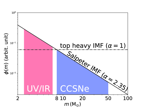
We combine two sets of observational constraints on the IMF, 1) cosmic CCSN explosion rates and 2) cosmic far UV radiation (and IR re-radiation) densities, which are sensitive to massive ($\simeq 8-50\,{\rm M}_{\odot}$) and moderately massive ($\simeq 2.5-7\,{\rm M}_{\odot}$) stars, respectively. We show these mass ranges in Figure 1. In this study, we constrain the IMF slope at $m>1\,{\rm M}_{\odot}$ with a freedom of redshift evolution. In this mass range, the IMF does not have turnovers which are found in the Milky Way (e.g. Kroupa 2001; Chabrier 2003). We present 1) and 2) in Sections 2.3 and 2.2, respectively. Section 2.4 discusses 2) with DSNB for the future studies.

It should be noted that the IMF should depend on galaxy properties including metallicities, star-formation rates, and masses. In this study, we aim at revealing the cosmic average IMF shape at each redshift that should depend on the cosmic average metallicities, star-formation rate densities, and mass densities, using the cosmic average CCSN rates and far UV+IR densities. It should be also noted that the time scale of the far UV and IR emission corresponds to the life-time of moderately-massive/massive stars,
$\sim 80\,(M/(7\,{\rm M}_{\odot}))^{-2.5}$ Myr (Hansen et al., 2004), where $M$ is the initial mass of the progenitor star. This time scale is much shorter than the time resolution of this study (i.e. CCSN-rate data binning size; Section 4.2), $\Delta z\sim 0.1$ corresponding to $\sim 500-1000$ Myr, at $z=0-2$. The far UV and IR emission are negligibly affected by the past star formation that was taken place in the different cosmic-average galaxy properties. For example, the results in Figure 2 do not change beyond the uncertainties of the IMF parameters if we vary the star formation history or stellar age.

In the analysis of Section 2.2, sample selections of galaxies are important. In our study, we use the cosmic average far-UV/IR luminosity densities that are derived from galaxy samples with completeness corrections, integrating the luminosity function at each redshift via star-formation rate densities. The luminosity functions are complete for a given luminosity, regardless of star-formation rates, stellar ages, and masses.

2.1 Parameterizing the IMF shape evolution

In this study, we assume a shape of the IMF as a single power-law with a slope $\alpha$. We define the minimum (maximum) mass of the IMF as $0.5\,{\rm M}_{\odot}$ ($200\,{\rm M}_{\odot}$), following the previous study of Ando et al. (2003).

On this assumption, the functional form of the IMF becomes

$$\phi(m,z)\propto m^{-\alpha}\,(0.5\,{\rm M}_{\odot}\leq m\leq 200\,{\rm M}_{\odot})$$ (1)

Here we include the evolution of $\alpha$ linearly depending on a redshift. Thus

$$\alpha=\alpha_{0}+\alpha_{z}\cdot z,$$ (2)

where $\alpha_{0}$ and $\alpha_{\rm z}$ are free parameters. We call these parameters the IMF parameters. In the case of the Salpeter IMF with no redshift evolution, the parameter set is $(\alpha_{0},\alpha_{\rm z})=(2.35,0)$. Although non power-law IMFs are important (e.g. Jermyn et al. 2018; Larson 1985; Lynden-Bell 1976; Sneppen et al. 2022; Conroy & van Dokkum 2012; Martín-Navarro et al. 2015), these IMFs are out of the scope of the main purpose of our this study.

2.2 Star formation rate density

A cosmic star formation rate density (SFRD) at a redshift $\psi(z)$ can be estimated with far UV radiation and IR re-radiation densities, which are $\rho_{\rm UV}$ and $\rho_{\rm IR}$, respectively. Because the SFRD depends on the IMF assumption, we convert an SFRD derived with the Salpeter IMF and the mass range of $0.1-100M_{\odot}$ (Madau & Dickinson, 2014) to those estimated with any IMFs and the mass range of $0.5-50M_{\odot}$ (Conroy et al., 2009; Conroy & Gunn, 2010), which conserves the observational quantities of $\rho_{\rm UV}$ and $\rho_{\rm IR}$ in the self-consistent manner. Here $\psi(z)$ is written as

$$\psi(z)=\mathcal{K}_{\rm UV}\rho_{\rm UV}+\mathcal{K}_{\rm IR}\rho_{\rm IR}~{}.$$ (3)

The coefficients $(\mathcal{K}_{\rm UV}$, $\mathcal{K}_{\rm IR})$ are determined with the population synthesis code created by Conroy et al. (2009) and Conroy & Gunn (2010). Here we define an cosmic SFRD estimated with the assumption of the Salpeter IMF $\psi^{\rm Sal}(z)$, and obtain

$$\psi^{\rm Sal}(z) = \mathcal{K}^{\rm Sal}_{\rm UV}\rho_{\rm UV}+\mathcal{K}^{\rm Sal}_{\rm IR}\rho_{\rm IR}$$ (4)

$$= 0.015\dfrac{(1+z)^{2.7}}{1+\left[(1+z)/2.9\right]^{5.6}}\,\,[{\rm M}_{\odot}/{\rm yr}/{\rm Mpc}^{-3}]\,,$$ (5)

where $\mathcal{K}^{\rm Sal}_{\rm UV}$ and $\mathcal{K}^{\rm Sal}_{\rm IR}$ are coefficients for the Salpeter IMF that are $3.30\times 10^{-28}\,[{\rm M}_{\odot}\,{\rm yr}^{-1}\,{\rm erg}^{-1}\,{\rm s}\,{\rm Hz}]$ and $3.46\times 10^{-10}\,[{\rm M}_{\odot}\,{\rm yr}^{-1}\,{\rm L}_{\odot}^{-1}]$, respectively.

The eq. (5) is derived with the best-fit function to many observational measurements of comic SFRDs obtained by Madau & Dickinson (2014) (MD14). As presented in Appendix B,

$$\psi(z)=\dfrac{\mathcal{K}_{\rm UV}}{\mathcal{K}_{\rm UV}^{\rm Sal}}\psi^{\rm Sal}(z)~{},$$ (6)

where we use the fact that the dependence of $\mathcal{K}_{\rm IR}/\mathcal{K}_{\rm UV}$ on $\alpha(z)$ is negligibly small, up to $\sim 3$%. The combination of eqs. 3 and 5 provides $\psi(z)$ as a function of redshift.

It is true that the IMF constraints from the SFR densities are affected by variables such as metallicity, typical star formation rate (SFR) and the mass of host halos at each redshift. In this paper, we do not intend to constrain the IMF redshift evolution at the fixed metallicity and SFR, but we want to discuss the IMF constraints on average at each redshift, including the effects from these parameters such as metallicity and SFR.

2.3 Number fraction of SNe to all stars

Progenitor stars of CCSNe have a $\gtrsim 10\%$ solar metallicity and an initial mass within a range of $8\,{\rm M}_{\odot}<m<50\,{\rm M}_{\odot}$ (Heger et al., 2003; Ando et al., 2003). One can calculate the ratio of CCSNe to all stars, $f(\alpha)$, using the IMF with

$$f(\alpha)=\dfrac{\int_{8\,{\rm M}_{\odot}}^{50\,{\rm M}_{\odot}}\phi(m,z)dm}{\int_{0.5\,{\rm M}_{\odot}}^{200\,{\rm M}_{\odot}}\phi(m,z)dm}~{},$$ (7)

In the case of the Salpeter IMF with no redshift evolution, the ratio is $f(\alpha)=0.0128$.

2.4 Neutrino spectrum

We use hydrodynamical simulations of CCSNe performed by Nakazato et al. (2013) to estimate the neutrino spectrum of a CCSN ${d^{2}\tilde{n}_{\nu}}/{dE_{\nu}dm}$. Here $E_{\nu}$ is the energy of neutrinos. These simulations have two major parameters, a metallicity of the progenitor star $Z$ and a revival time scale of shock waves $t_{\rm revive}$. We assume $Z$ as the solar metallicity $Z_{\odot}$ for simplicity. We adopt $t_{\rm revive}=300\,{\rm ms}$ that is derived by observations of SN1987A (Beacom, 2010).

In the high redshift Universe, one cannot spatially resolve a CCSN. By using the expected spectra of the DSNB from the simulation results of Nakazato et al. (2013), we derive the IMF-weighted spectrum of neutrinos ${d\tilde{n}_{\nu}}/{dE_{\nu}}$ expressed as

$$\dfrac{d\tilde{n}_{\nu}}{dE_{\nu}}(E_{\nu},z)=\int_{8\,{\rm M}_{\odot}}^{50\,{\rm M}_{\odot}}\dfrac{d^{2}\tilde{n}_{\nu}}{dE_{\nu}dm}\phi(m,z)dm~{},$$ (8)

Here we adopt the instantaneous recycling approximation, in which massive stars $>1\,{\rm M}_{\odot}$ finish their lives instantaneously (Searle & Sargent, 1972). The spectrum of the DSNB $dn_{\nu}/{dE_{\nu}}$ is derived as (Ando et al. 2003; Beacom 2010)

$$\dfrac{dn_{\nu}}{dE}(E_{\nu})=\int_{0}^{+\infty}(1+z)f(\alpha)\psi(z)\left\{\dfrac{d\tilde{n}_{\nu}}{dE_{\nu}}[(1+z)E_{\nu},z]\right\}H(z)dz\,,$$ (9)

where $H(z)$ is the Hubble parameter at $z$. The term $(1+z)E_{\nu}$ corresponds to the energy of redshifted neutrinos. The term $f(\alpha)\psi(z)$ is the cosmic event rate of CCSNe per unit comoving volume.

The HK is sensitive to DSNBs at the energy range $19.7-30.0\,{\rm MeV}$ (Hyper-Kamiokande Proto-Collaboration et al., 2018). For the HK, the neutrino flux of DSNBs $n_{\nu}^{\rm HK}$ is

$$n_{\nu}^{\rm HK}=\int_{19.7\,{\rm MeV}}^{30.0\,{\rm MeV}}\dfrac{dn_{\nu}}{dE_{\nu}}(E_{\nu})dE_{\nu}$$ (10)

With the eq. (10), Hyper-Kamiokande Proto-Collaboration et al. (2018) estimate the number of DSNB neutrinos to be 140 with the 5.7 $\sigma$ non-zero significance level under the assumption of the Salpter IMF with no redshift evolution and a 20-year operation of the HK. This number highly depends on the cosmic SFRD. In the Hyper-Kamiokande Proto-Collaboration et al. (2018), the SFRD is significantly underestimated compared with recent observational results claimed in Madau & Dickinson (2014), hereafter MD14. We expect that the HK will detect 280 DSNB neutrinos at the 7.4 $\sigma$ non-zero significance level over a 20-year operation in the case that the cosmic SFRD is given by MD14 under the assumptions of the Salpeter IMF with no redshift evolution . We estimate the neutrino flux of the 280 DSNB neutrino detections to be $0.33\,\pm 0.04\,{\rm cm}^{-2}{\rm s}^{-1}$, following the calculations of Ando et al. (2003). We use this neutrino flux and uncertainty to forecast constraints on $(\alpha_{0},\alpha_{\rm z})$, assuming this neutrino flux uncertainty independent of the neutrino flux.

Figure 2: Constraint on a parameter set of the IMF with optical number counts of SNe up to date. The contours correspond to $1,2$ and $3\,\sigma$ CL from the inside to outside (blue, red and green lines). The Salpeter IMF with no redshift evolution is represented with a cross mark ”x” at the center.

Figure 3: Forecast of constraint with the Roman telescope. The contours (blue) are defined as the same as Figure 2. The contours in Figure 2 are shown with gray lines.

Figure 4: Forecast of constraint with the HK. The contours (blue) are defined as the same as Figure 2. The contours in Figure 2 are shown with gray lines.

3 Result

3.1 CCSN number counts

3.1.1 IMF constrained by the existing observations

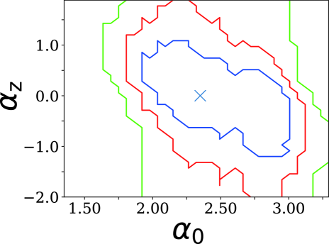
We use the CCSN number counts obtained by two observational studies of Mattila et al. (2012) and Dahlen et al. (2012), which directly constrain $f(\alpha)\psi(z)$ as a function of redshift. The results of these two observational studies are reliable, because the CCSNe counts are corrected for dust extinction. Moreover, more than half of the CCSNe are spectroscopically confirmed. By comparing the CCSNe number counts with our predictions, $f(\alpha)\psi(z)$, at each redshift, we set a constraint on the parameter space $(\alpha_{0},\alpha_{\rm z})$ as shown in Figure 2. One can see a decreasing trend in Figure 2. If $\alpha_{0}$ increases, $\alpha_{\rm z}$ decreases, because a large number of massive stars are needed at high redshift to explain the observed CCSN number counts in the case of the higher value of $\alpha_{0}$ (resulting in a smaller number of massive stars at $z\simeq 0$). Our result is consistent with the Salpeter IMF with no redshift evolution albeit with the large uncertainty. This large uncertainty originates from large error bars of the number counts of CCSNe at a redshift range $z\gtrsim 0.5$ in Dahlen et al. (2012). Although we only use the results of optical observations available up to date, we exclude a top (bottom) heavy IMF such as $\alpha<1.8$ ($\alpha>3.1$) in the local Universe at the 2 $\sigma$ CL. Our constraint is consistent with the previous studies such as Martín-Navarro et al. (2015) and Conroy & van Dokkum (2012).

3.1.2 IMF constrained by future observations

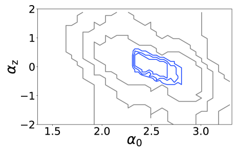
The Roman Space Telescope is scheduled to be launched in the middle of the 2020s. The Roman Space Telescope has the one hundred times larger field of view than that of the HST. Hounsell et al. (2018) shows that approximately 540 CCSNe will be identified. We assume that the uncertainty of the number counts follows the Poisson statistics. We obtain the forecast as shown in Figure 3. We can narrow the $2\sigma$ error contour down to $2.25<\alpha_{0}<2.70$ and $|\alpha_{\rm z}|<0.5$. Here we assume the fiducial values are those for the Salpeter IMF with no redshift evolution.

3.2 Neutrino fluxes measured in the future

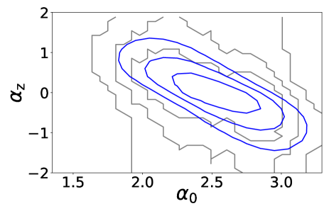
The HK is now under construction and planned to be operated from 2027. By the 20 year operation of the HK, the IMF parameters are constrained as shown in Figure 4. We obtain the forecast of $2.05<\alpha_{0}<3.00$ and $|\alpha_{\rm z}|<0.9$ at the 2 $\sigma$ CL. The value of $\alpha_{\rm z}$ is constrained better than the one of the present SN survey results (Figure 2). These improvements of the parameter constraints will be accomplished mainly due to the increase of the detection number of the DSNB neutrinos originated from $z\simeq 1-2$ Universe .

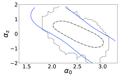
The neutrino fluxes from CCSNe can be changed by assumptions that include an approximation of gas motions around the progenitor core and a choice of the equation of state . A systematic uncertainty of the neutrino flux raised by the assumptions is estimated to be $\sim 50$% (private communications with K. Kotake, see also Mathews et al. (2020)). We include the systematic uncertainty into our model calculations, and show the contours of the forecast in Figure 5. Figure 5 indicates that one rules out the top heavy IMF such as $\alpha_{0}<1.6$ with the $2\sigma$ CL (confidence level) even in the case with the systematic uncertainty. In Figure 5, the forecast contours with the systematic uncertainty (blue line) is as large as the contour obtained by this study with the optical number counts (gray lines; Section 3.1.1). We discuss the large uncertainty raised by the systematics in Section 4.2.2.

Figure 5: Uncertainty of the parameter estimation from the simulation uncertainty (blue line) . All lines correspond to the $2\,\sigma$ CL. The fiducial case is shown with black dot-dashed line, which is shown in figure 4. The contours in Figure 2 are shown with gray lines.

4 Discussion

4.1 IMF constrained by this study

As shown in Section 3.1.1, the cosmic IMF at $z=0$ falls in $1.8<\alpha<3.2$ with $2\,\sigma$ CL. This result excludes the top heavy IMF such as $\alpha=1$ more than $4\,\sigma$ CL in the local Universe. This result suggests that the star formation mechanism in distant Universe is consistent with that in local Universe, which are claimed in Inutsuka (2001) and Inutsuka et al. (2015). However, the uncertainties of $\alpha_{0}$ and $\alpha_{\rm z}$ are large to discuss the IMF at high redshifts because the current results depend on only several tens CCSN observations.

4.2 IMF constrained in the future

4.2.1 CCSN number counts

In the near future, the forecast of the constraint is $2.2<\alpha<2.7$ ($1.9<\alpha<3.1$) at a redshift $z=0$ ($z=1$) .

4.2.2 Neutrino fluxes

Following the discussion in Section 4.2.1, the forecast of the HK is $2.25<\alpha<3.02$ $(1.35<\alpha<3.92)$ at a redshift $z=0$ ($z=1$).

Ideally, a strong constraint on the IMF parameters will be set as shown in Figure 4. Note that the forecast of the IMF parameter constraints does not include in the systematic uncertainty raised by the theoretical model that bridges between the CCSN explosion and the neutrino flux (Nakazato et al., 2013). If the systematic uncertainty of the theoretical model is considered, the forecast of the IMF parameter constraints with the future HK data is as large as the present IMF parameter constraints (Figure 5). Accomplishing the parameter constraints shown in Figure 4, one needs to reduce the systematic uncertainty of theoretical models. One can expect that the model of the CCSN explosion can be improved by fast-computational resources and new computation schemes, which will narrow the systematic uncertainty.

Comparing the computational speed of the best super computers in years of 2021 and 2001 on the basis of TOP500 ranking , one can find that the one of year 2021 has a speed thirty six thousand times faster than the one of year 2001. The computational scheme of the simulations of CCSNe has also been improved in the same period (2001-2021). Now theorists have realized spontaneous explosions of CCSNe, three dimensional simulations of CCSNe, and the detailed neutrino transfer in the dense matter around the core of CCSNe, while none of them has been conducted in 2001. Similarly, we expect to see significant improvements in the processing speed and the calculation scheme in the forthcoming 30 years of the HK construction and operation. In fact, Bastian et al. (2018) show that it costs several million node-hours (SuperMUC/Germany) to conduct 3-D CCSN simulations, today’s state-of-the-art CCSN simulations, with full neutrino transports (see Couch et al. 2020). If one performs 3-D neutrino transport simulations that accomplish the accuracy of 50% in the CCSN neutrino emission estimates with the top-ranked supercomputer today (Fugaku/Japan), it takes more than one years that is not realistic. Note that the Bastian et al.’s simulations took approximately 170 years with the top-ranked supercomputer 20 years ago (ASCI White/the United States), but completes in less than 2 days with Fugaku/Japan. Such a computational power evolution towards the future will allow us to realize the high-resolution magneto-hydrodynamical general relativistic neutrino-driven core-collapse supernova explosion simulations probably in $\sim 0.1$ years . If the systematic uncertainty of the theoretical model becomes very small, the IMF parameter constraints of Figure 4 will be obtained.

There is a future plan that the second HK (HK2) will be constructed in Korea. The HK2 will be used to improve the detectablity of proton decays and the determination of the parameters of neutrinos. The design and performance of the HK2 are supposed to be exactly the same as those of the HK (Hyper-Kamiokande Proto-Collaboration et al., 2018). If the HK2 observes DSNB neutrinos for 20 years, the number of DSNB neutrinos detections will be doubled. Assuming the improvements of Poisson noise by the doubled sample, we expect that the IMF constraints will be narrowed to $2.1<\alpha_{0}<2.9$ and $|\alpha_{\rm z}|<0.7$ as shown in Figure 6.

4.2.3 Implication to be obtained by the future observations

In Section 4.2, we find that the IMF constraints from DSNB neutrinos ($2.25<\alpha<3.02$) are not strong as those of CCSN number counts ($2.2<\alpha<2.7$). The neutrino constraints are placed with spectra of the DSNB neutrinos integrated over redshift, while CCSN number counts are obtained as a function of redshift. Although the CCSN number counts and DSNB neutrino measurements both provide the constraints on the IMF, independent observational tests are needed to reliably understand the IMF and its evolution.

We show the forecast of constraints obtained with CCSN number counts of the Roman space telescope (Figure 3) and the HK+HK2 (Figure 6). If one obtains these constraints on the IMF parameters in the future, the Roman and HK+HK2 observations can test the existence of top-heavy IMFs of $\alpha=1$ at $z\gtrsim 2$ such suggested in previous studies (e.g. Baugh et al. 2005; Aoyama et al. 2019)

. If the HK+HK2 detects no DSNB neutrinos, the HK+HK2 will rule out the Salpeter IMF with no redshift evolution.

Figure 6: The forecast of constraint with the HK and the HK2. The contours are defined as the same as in Figure 2. The contours (blue) in Figure 2 are shown with gray lines.

5 Conclusion

We suggest a new method to constrain average IMF shapes of galaxies. We include the linear evolution of the IMF slope, $\alpha$, by redshift. The IMF parameters can be constrained by the CCSN number counts and DSNB neutrino numbers. With the currently available observational data of the CCSN number counts, we obtain $1.8<\alpha_{0}<3.1$ at the $2\,\sigma$ CL (Figure 2). The CCSN number counts suggest that the IMF in the local Universe is consistent with the Salpeter IMF with no redshift evolution. Moreover, top-heavy IMFs in the local Universe are ruled out by the CCSN number counts. However, redshift evolutions of the IMF shape are not identified with the current observational data due to the small sample of the CCSNe in the previous studies.

In the future, Roman space telescope will identify CCSNe ten times larger than the number of currently available CCSNe. The large number of CCSNe will determine the IMF parameters with high accuracy (Figure 3). The HK and HK+HK2 can also place a constraint on the IMF parameters with the number of DSNB neutrinos detected over the 20-year operation (Figure 4). This constraint is independent from the one of the CCSN number counts. If there are no systematic errors more than those suggested in Bays et al. (2012) we expect to place the constraint on the IMF parameters over the 20-year operation of the HK (Figures 4 and 6). With these constraints, one can test the top heavy IMF at high redshift such suggested by Baugh et al. (2005) and Aoyama et al. (2019) .

6 acknowledgements

We acknowledge an anonymous referee for providing useful comments and discussions. Numerical computations were carried out on analysis servers and Cray XC50 at the Center for Computational Astrophysics (CfCA), National Astronomical Observatory of Japan, Yukawa-21 at the Yukawa Institute Computer Facility in Kyoto University. SA acknowledges the CfCA for providing the computing resources of analysis servers and Cray XC50. This work is supported by the World Premier International Research Center Initiative (WPI Initiative), MEXT, Japan, as well as KAKENHI Grant-in-Aid for Scientific Research (A) (20H00180 and 21H04467) through the Japan Society for the Promotion of Science (JSPS). YH acknowledges support from the JSPS KAKENHI grant No. 19J01222 and 21K13953. This work is supported by the joint research program of the Institute for Cosmic Ray Research (ICRR), the University of Tokyo.

7 Appendix

By changing the IMF, the estimated $\psi(z)$ from UV/IR flux is changed. By using the fact that a coefficient $\mathcal{K}_{\rm IR}/\mathcal{K}_{\rm UV}$ does not depend on $\alpha$ with a few percent accuracy, we can obtain $\psi(z)$ from $\psi_{\rm Sal}(z)$ as follows.

$$\psi(z) = \mathcal{K}_{\rm UV}\rho_{\rm UV}+\mathcal{K}_{\rm IR}\rho_{\rm IR}$$ (11)

$$= \mathcal{K}_{\rm UV}\rho_{\rm UV}+(\mathcal{K}_{\rm IR}/\mathcal{K}_{\rm UV})\mathcal{K}_{\rm UV}\rho_{\rm IR}$$ (12)

$$\simeq \mathcal{K}_{\rm UV}\rho_{\rm UV}+(\mathcal{K}_{\rm IR}^{\rm Sal}/\mathcal{K}_{\rm UV}^{\rm Sal})\mathcal{K}_{\rm UV}\rho_{\rm IR}$$ (13)

$$= \mathcal{K}_{\rm UV}/\mathcal{K}_{\rm UV}^{\rm Sal}\left(\mathcal{K}_{\rm UV}^{\rm Sal}\rho_{\rm UV}+\mathcal{K}_{\rm IR}^{\rm Sal}\rho_{\rm IR}\right)$$ (14)

$$= \mathcal{K}_{\rm UV}/\mathcal{K}_{\rm UV}^{\rm Sal}\psi^{\rm Sal}(z)\,.$$ (15)

References

- Ando et al. (2003) Ando, S., Sato, K., & Totani, T. 2003, Astroparticle Physics, 18, 307, doi: 10.1016/S0927-6505(02)00152-4
- André et al. (2010) André, P., Men’shchikov, A., Bontemps, S., et al. 2010, A&A, 518, L102, doi: 10.1051/0004-6361/201014666
- Annala et al. (2018) Annala, E., Gorda, T., Kurkela, A., & Vuorinen, A. 2018, Phys. Rev. Lett., 120, 172703, doi: 10.1103/PhysRevLett.120.172703
- Aoyama et al. (2019) Aoyama, S., Hirashita, H., Lim, C.-F., et al. 2019, MNRAS, 484, 1852, doi: 10.1093/mnras/stz021
- Baldry & Glazebrook (2003) Baldry, I. K., & Glazebrook, K. 2003, ApJ, 593, 258, doi: 10.1086/376502
- Bastian et al. (2010) Bastian, N., Covey, K. R., & Meyer, M. R. 2010, ARA&A, 48, 339, doi: 10.1146/annurev-astro-082708-101642
- Baugh et al. (2005) Baugh, C. M., Lacey, C. G., Frenk, C. S., et al. 2005, MNRAS, 356, 1191, doi: 10.1111/j.1365-2966.2004.08553.x
- Bauswein et al. (2017) Bauswein, A., Just, O., Janka, H.-T., & Stergioulas, N. 2017, ApJ, 850, L34, doi: 10.3847/2041-8213/aa9994
- Bays et al. (2012) Bays, K., Iida, T., Abe, K., et al. 2012, Phys. Rev. D, 85, 052007, doi: 10.1103/PhysRevD.85.052007
- Beacom (2010) Beacom, J. F. 2010, Annual Review of Nuclear and Particle Science, 60, 439, doi: 10.1146/annurev.nucl.010909.083331
- Chabrier (2003) Chabrier, G. 2003, PASP, 115, 763, doi: 10.1086/376392
- Conroy & Gunn (2010) Conroy, C., & Gunn, J. E. 2010, ApJ, 712, 833, doi: 10.1088/0004-637X/712/2/833
- Conroy et al. (2009) Conroy, C., Gunn, J. E., & White, M. 2009, ApJ, 699, 486, doi: 10.1088/0004-637X/699/1/486
- Conroy & van Dokkum (2012) Conroy, C., & van Dokkum, P. G. 2012, ApJ, 760, 71, doi: 10.1088/0004-637X/760/1/71
- Couch et al. (2020) Couch, S. M., Warren, M. L., & O’Connor, E. P. 2020, ApJ, 890, 127, doi: 10.3847/1538-4357/ab609e
- Cromartie et al. (2020) Cromartie, H. T., Fonseca, E., Ransom, S. M., et al. 2020, Nature Astronomy, 4, 72, doi: 10.1038/s41550-019-0880-2
- Dahlen et al. (2012) Dahlen, T., Strolger, L.-G., Riess, A. G., et al. 2012, ApJ, 757, 70, doi: 10.1088/0004-637X/757/1/70
- Davé (2008) Davé, R. 2008, MNRAS, 385, 147, doi: 10.1111/j.1365-2966.2008.12866.x
- Hansen et al. (2004) Hansen, C. J., Kawaler, S. D., & Trimble, V. 2004, Stellar interiors : physical principles, structure, and evolution
- Heger et al. (2003) Heger, A., Fryer, C. L., Woosley, S. E., Langer, N., & Hartmann, D. H. 2003, ApJ, 591, 288, doi: 10.1086/375341
- Hirata et al. (1987) Hirata, K., Kajita, T., Koshiba, M., et al. 1987, Phys. Rev. Lett., 58, 1490, doi: 10.1103/PhysRevLett.58.1490
- Hounsell et al. (2018) Hounsell, R., Scolnic, D., Foley, R. J., et al. 2018, ApJ, 867, 23, doi: 10.3847/1538-4357/aac08b
- Hyper-Kamiokande Proto-Collaboration et al. (2018) Hyper-Kamiokande Proto-Collaboration, :, Abe, K., et al. 2018, arXiv e-prints, arXiv:1805.04163. https://arxiv.org/abs/1805.04163
- Inutsuka (2001) Inutsuka, S.-i. 2001, ApJ, 559, L149, doi: 10.1086/323786
- Inutsuka et al. (2015) Inutsuka, S.-i., Inoue, T., Iwasaki, K., & Hosokawa, T. 2015, A&A, 580, A49, doi: 10.1051/0004-6361/201425584
- Inutsuka & Miyama (1997) Inutsuka, S.-i., & Miyama, S. M. 1997, ApJ, 480, 681, doi: 10.1086/303982
- Jermyn et al. (2018) Jermyn, A. S., Steinhardt, C. L., & Tout, C. A. 2018, MNRAS, 480, 4265, doi: 10.1093/mnras/sty2123
- Kajita (1999) Kajita, T. 1999, Nuclear Physics B Proceedings Supplements, 77, 123, doi: 10.1016/S0920-5632(99)00407-7
- Kippenhahn et al. (2012) Kippenhahn, R., Weigert, A., & Weiss, A. 2012, Stellar Structure and Evolution, doi: 10.1007/978-3-642-30304-3
- Könyves et al. (2010) Könyves, V., André, P., Men’shchikov, A., et al. 2010, A&A, 518, L106, doi: 10.1051/0004-6361/201014689
- Könyves et al. (2015) —. 2015, A&A, 584, A91, doi: 10.1051/0004-6361/201525861
- Kroupa (2001) Kroupa, P. 2001, MNRAS, 322, 231, doi: 10.1046/j.1365-8711.2001.04022.x
- Kroupa et al. (2013) Kroupa, P., Weidner, C., Pflamm-Altenburg, J., et al. 2013, in Planets, Stars and Stellar Systems. Volume 5: Galactic Structure and Stellar Populations, ed. T. D. Oswalt & G. Gilmore, Vol. 5, 115, doi: 10.1007/978-94-007-5612-0_4
- Larson (1985) Larson, R. B. 1985, MNRAS, 214, 379, doi: 10.1093/mnras/214.3.379
- Lynden-Bell (1976) Lynden-Bell, D. 1976, MNRAS, 174, 695, doi: 10.1093/mnras/174.3.695
- Madau & Dickinson (2014) Madau, P., & Dickinson, M. 2014, ARA&A, 52, 415, doi: 10.1146/annurev-astro-081811-125615
- Martín-Navarro et al. (2015) Martín-Navarro, I., Pérez-González, P. G., Trujillo, I., et al. 2015, ApJ, 798, L4, doi: 10.1088/2041-8205/798/1/L4
- Mathews et al. (2020) Mathews, G. J., Boccioli, L., Hidaka, J., & Kajino, T. 2020, Modern Physics Letters A, 35, 2030011, doi: 10.1142/S0217732320300116
- Mattila et al. (2012) Mattila, S., Dahlen, T., Efstathiou, A., et al. 2012, ApJ, 756, 111, doi: 10.1088/0004-637X/756/2/111
- Nakazato et al. (2013) Nakazato, K., Sumiyoshi, K., Suzuki, H., et al. 2013, ApJS, 205, 2, doi: 10.1088/0067-0049/205/1/2
- Raffelt (1996) Raffelt, G. G. 1996, Stars as laboratories for fundamental physics : the astrophysics of neutrinos, axions, and other weakly interacting particles
- Salpeter (1955) Salpeter, E. E. 1955, ApJ, 121, 161, doi: 10.1086/145971
- Searle & Sargent (1972) Searle, L., & Sargent, W. L. W. 1972, ApJ, 173, 25, doi: 10.1086/151398
- Sneppen et al. (2022) Sneppen, A., Steinhardt, C. L., Hensley, H., et al. 2022, ApJ, 931, 57, doi: 10.3847/1538-4357/ac695e
- van Dokkum et al. (2017) van Dokkum, P., Conroy, C., Villaume, A., Brodie, J., & Romanowsky, A. J. 2017, ApJ, 841, 68, doi: 10.3847/1538-4357/aa7135
- van Dokkum & Conroy (2010) van Dokkum, P. G., & Conroy, C. 2010, Nature, 468, 940, doi: 10.1038/nature09578