capbtabboxtable[][\FBwidth]
Qimera: Data-free Quantization with Synthetic Boundary Supporting Samples
Abstract
Model quantization is known as a promising method to compress deep neural networks, especially for inferences on lightweight mobile or edge devices. However, model quantization usually requires access to the original training data to maintain the accuracy of the full-precision models, which is often infeasible in real-world scenarios for security and privacy issues. A popular approach to perform quantization without access to the original data is to use synthetically generated samples, based on batch-normalization statistics or adversarial learning. However, the drawback of such approaches is that they primarily rely on random noise input to the generator to attain diversity of the synthetic samples. We find that this is often insufficient to capture the distribution of the original data, especially around the decision boundaries. To this end, we propose Qimera, a method that uses superposed latent embeddings to generate synthetic boundary supporting samples. For the superposed embeddings to better reflect the original distribution, we also propose using an additional disentanglement mapping layer and extracting information from the full-precision model. The experimental results show that Qimera achieves state-of-the-art performances for various settings on data-free quantization. Code is available at https://github.com/iamkanghyunchoi/qimera.
1 Introduction
Among many neural network compression methodologies, quantization is considered a promising direction because it can be easily supported by accelerator hardwares [1] than pruning [2] and is more lightweight than knowledge distillation [3]. However, quantization generally requires some form of adjustment (e.g., fine-tuning) using the original training data [4, 5, 6, 7, 8] to restore the accuracy drop due to the quantization errors. Unfortunately, access to the original training data is not always possible, especially for deployment in the field, for many reasons such as privacy and security. For example, the data could be medical images of patients, photos of confidential products, or pictures of military assets.
Therefore, data-free quantization is a natural direction to achieve a highly accurate quantized model without accessing any training data. Among many excellent prior studies [9, 10, 11, 12], generative methods [13, 14, 15] have recently been drawing much attention due to their superior performance. Generative methods successfully generate synthetic samples that resemble the distribution of the original dataset and achieve high accuracy using information from the pretrained full-precision network, such as batch-normalization statistics [15, 13] or intermediate features [14].
However, a significant gap still exists between data-free quantized models and quantized models fine-tuned with original data. What is missing from the current generative data-free quantization schemes? We hypothesize that the synthetic samples of conventional methods lack boundary supporting samples [16], which lie on or near the decision boundary of the full-precision model and directly affect the model performance. The generator designs are often based on conditional generative adversarial networks (CGANs) [17, 18] that take class embeddings representing class-specific latent features. Based on these embeddings as the centroid of each class distribution, generators rely on the input of random Gaussian noise vectors to gain diverse samples. However, one can easily deduce that random noises have difficulty reflecting the complex class boundaries. In addition, the weights and embeddings of the generators are trained with cross-entropy (CE) loss, further ensuring that these samples are well-separated from each other.
In this work, we propose Qimera, a method for data-free quantization employing superposed latent embeddings to create boundary supporting samples. First, we conduct a motivational experiment to confirm our hypothesis that samples near the boundary can improve the quantized model performance. Then, we propose a novel method based on inputting superposed latent embeddings into the generator to produce synthetic boundary supporting samples. In addition, we provide two auxiliary schemes for flattening the latent embedding space so that superposed embeddings could contain adequate features.
Qimera achieves significant performance improvement over the existing techniques. The experimental results indicate that Qimera sets new state-of-the-art performance for various datasets and model settings for the data-free quantization problem. Our contributions are summarized as the following:
-
•
We identify that boundary supporting samples form an important missing piece of the current state-of-the-art data-free compression.
-
•
We propose using superposed latent embeddings, which enables a generator to synthesize boundary supporting samples of the full-precision model.
-
•
We propose disentanglement mapping and extracted embedding initialization that help train a better set of embeddings for the generator.
-
•
We conduct an extensive set of experiments, showing that the proposed scheme outperforms the existing methods.
2 Related Work
2.1 Data-free Compression
Early work on data-free compression has been led by knowledge distillation [3], which usually involves pseudo-data created from teacher network statistics [19, 20]. Lopes et al. [19] suggested generating pseudo-data from metadata collected from the teacher in the form of activation records. Nayak et al. [20] proposed a similar scheme but with a zero-shot approach by modeling the output space of the teacher model as a Dirichlet distribution, which is taken from model weights. More recent studies have employed generator architectures similar to GAN [21] to generate synthetic samples replacing the original data [22, 23, 24, 25]. In the absence of the original data for training, DAFL [22] used the teacher model to replace the discriminator by encouraging the outputs to be close to a one-hot distribution and by maximizing the activation counts. KegNet [26] adopted a similar idea and used a low-rank decomposition to aid the compression. Adversarial belief matching [23] and data-free adversarial distillation [24] methods suggested adversarially training the generator, such that the generated samples become harder to train. One other variant is to modify samples directly using logit maximization as in DeepInversion [25]. While this approach can generate images that appear natural to a human, it has the drawback of skyrocketing computational costs because each image must be modified using backpropagation.
Data-free quantization is similar to data-free knowledge distillation but is a more complex problem because quantization errors must be recovered. The quantized model has the same architecture as the full-precision model; thus, the early methods of post-training quantization were focused on how to convert the full-precision weights into quantized weights by limiting the range of activations [9, 12], correcting biases [9, 10], and equalizing the weights [10, 12]. ZeroQ [15] pioneered using synthetic data for data-free quantization employing statistics stored in batch-normalization layers. GDFQ [13] added a generator close to the ACGAN [18] to generate better synthetic samples, and AutoReCon [27] suggests a better performing generator found by neural architecture search. In addition, DSG [28] further suggests relaxing the batch-normalization statistics alignment to generate more diverse samples. ZAQ [14] adopted adversarial training of the generator on the quantization problem and introduced intermediate feature matching between the full-precision and quantized model. However, none of these considered aiming to synthesize boundary supporting samples of the full-precision model. Adversarial training of generators have a similar purpose, but it is fundamentally different from generating boundary supporting samples. In addition, adversarial training can be sensitive to hyperparameters and risks generating samples outside of the original distributions [29]. To the extent of our knowledge, this work is the first to propose using superposed latent embeddings to generate boundary supporting samples explicitly for data-free quantizations.
2.2 Boundary Supporting Samples
In the context of knowledge distillation, boundary supporting samples [16] are defined as samples that lie near the decision boundary of the teacher models. As these samples contain classification information about the teacher models, they can help the student model correctly mimic the teacher’s behavior. Heo et al. [16] applied an adversarial attack [30] to generate boundary supporting samples and successfully demonstrated that they improve knowledge distillation performance. In AMKD [31], triplet loss was used to aid the student in drawing a better boundary. Later, DeepDig [32] devised a refined method for generating boundary supporting samples and analyzed their characteristics by defining new metrics. Although boundary supporting samples have been successful for many problems, such as domain adaptation [33] and open-set recognition [34], they have not yet been considered for data-free compression.
| Data | Accuracy | Data-free |
| Fine-tuned with Original data | 68.28% | ✗ |
| Synthetic samples | 63.39% | ✓ |
| Synthetic + unconfusing real samples | 63.91% (+0.52) | ✗ |
| Synthetic + confusing real samples | 65.75% (+2.36) | ✗ |
| Qimera (This work) | 65.10% (+1.71) | ✓ |
3 Motivational Experiment
To explain the discrepancy between the accuracy of the model fine-tuned with the original training data and the data-free quantized models, we hypothesized that the synthetic samples from generative data-free quantization methods lack samples near the decision boundary. To validate this hypothesis, we designed an experiment using the CIFAR-100 [35] dataset with the ResNet-20 network [36].
First, we forwarded images in the dataset into the pre-trained full-precision ResNet-20. Among these, we selected 1500 samples (3% of the dataset, 15 samples per class) from samples where the highest confidence value was lower than 0.25, forming a group of ‘confusing’ samples. Then, we combined the confusing samples with synthetic samples generated from a previous study [13] to fine-tune the quantized model with 4-bit weights and 4-bit activations. We also selected as a control group an equal number of random samples from the images classified as unconfusing and fine-tuned the quantized model using the same method.
The results are presented in Table 1. The quantized model with synthetic + unconfusing real samples exhibited only 0.52%p increase in the accuracy from the baseline. In contrast, adding confusing samples provided 2.36%p improvement, filling almost half the gap towards the quantized model fine-tuned with the original data. These results indirectly validate that the synthetic samples suffer from a lack of confusing samples (i.e., boundary supporting samples). We aim to address the issue in this paper. As we indicate in Section 5, Qimera achieves a 1.71%p performance gain for the same model in a data-free setting, close to that of the addition of confusing synthetic samples.
4 Generating Boundary Supporting Samples with Superposed Latent Embeddings
4.1 Baseline Generative Data-free Quantization
Recent generative data-free quantization schemes [13, 14] employ a GAN-like generator to create synthetic samples. In the absence of the original training samples, the generator attempts to generate synthetic samples so that the quantized model can mimic the behavior of the full-precision model . For example, in GDFQ [13], the loss function is
| (1) |
where the first term guides the generator to output clearly classifiable samples, and the second term aligns the batch-normalization statistics of the synthetic samples with those of the batch-normalization layers in the full-precision model. In another previous work ZAQ [14],
| (2) |
where the first term separates the prediction outputs of and , and the second term separates the feature maps produced by and . These two losses let the generator be adversarially trained and allow it to determine samples where cannot mimic adequately. Lastly, the third term maximizes the activation map values of so that the created samples do not drift too far away from the original dataset.
The quantized model is usually jointly trained with , such that
| (3) |
for GDFQ, and
| (4) |
for ZAQ, respectively, where from Eq. 3 is the usual KD loss with Kullback-Leibler divergence.
with Gaussian noise.
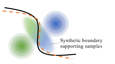
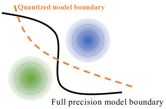
While these two methods exhibit great performance, they both model the distribution of per-class embeddings in the latent input space as a Gaussian distribution, and generate diverse samples using random Gaussian noise inputs. However, based on the Gaussian distribution, it is difficult to correctly reflect the boundary between the two different classes, especially when all samples have one-hot labels. Figure 1 visualizes such problems in a simplified two-dimensional space. With samples generated from gaussian noise (Figure 1(a)), the two per-class distributions are far away, and a void exists between the two classes (see Figure 3(b) for plots from experimental data). This can cause the decision boundaries to be formed at nonideal regions. One alternative is to use noise with higher variance, but the samples would overlap on a large region, resulting in too many samples with incorrect labels.
Furthermore, in the above approaches, the loss terms of Eqs. 1 and 2 such as and encourage the class distributions to be separated from each other. While this is beneficial for generating clean, well-classified samples, it also prevents generating samples near the decision boundary, which is necessary for training a good model [16, 31]. Therefore, in this paper, we focus on methods to generate synthetic samples near the boundary from the full-precision model (Figure 1(b)).
4.2 Superposed Latent Embeddings
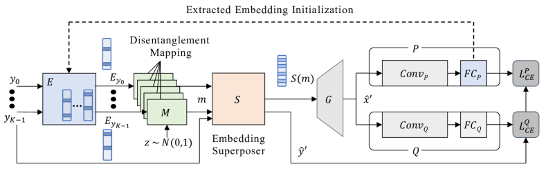
The overview of Qimera is presented in Figure 2. Often, generators use learned embeddings to create samples of multiple classes [18, 37]. Given an input one-hot label representing one of classes and a random noise vector , a generator uses an embedding layer to create a synthetic sample :
| (5) |
To create boundary supporting samples, we superpose the class embeddings so that the generated samples have features lying near the decision boundaries of . With two embeddings superposed, new synthetic sample becomes
| (6) |
To avoid too many confusing samples from complicating the feature space, we also apply soft labels in the same manner as a regularizer:
| (7) |
Generalizing to embeddings, Eqs. 6 and 7 become
| (8) | |||||
| (9) |
where has embeddings from as the column vectors (i.e., ), and is a superposer function. Applying this to existing methods is straightforward and incurs only a small amount of computational overhead. Similar to knowledge distillation with boundary supporting samples [16, 31], the superposed embeddings are supposed to help transfer the decision boundary of the full precision (teacher) model to the quantized (student) model.
Although the superposed embedding scheme alone produces a substantial amount of performance gains, the generator embedding space is often not flat enough [38]; therefore, linearly interpolating them can result in unnatural samples [39]. To mitigate this, the embedding space used in Qimera should possess two characteristics. First, the embedding space should be as flat as possible so that the samples generated from Eq. 8 reflect the intermediate points in the feature space. Second, the individual embeddings should still be sufficiently distinct from each other, correctly representing the distance between each class distribution. In the remaining two subsections, we describe our strategies for enforcing the embeddings to contain the above characteristics.
4.3 Disentanglement Mapping
To perform superposing in a flatter manifold, we added a learnable mapping function before the embeddings are superposed, where is the embedding dimension and is the dimension of the target space. Thus, from Eq. 8 becomes , where . Although we do not add any specific loss that guides the output space of to be flat, training to match the output of the full-precision model (i.e., ) using the superposed encourages to map the input to a flatter space. In practice, we modeled as a single-layer perceptron, which we call the disentanglement mapping layer. The experimental results from Section 5 demonstrate that the disentanglement mapping provides a considerable amount of performance gain.
4.4 Extracted Embedding Initialization
For the embeddings to be flat, we want the distributions of the embeddings fused with noise to be similar to the feature space. For this purpose, we utilize the fully connected layer of the full precision model . Given , the output features of the full-precision model before the last fully connected layer, we minimize , where is the number of classes, is the input of the generator, and is some distance metric. We do not have knowledge of the distribution of ; thus, we modeled it as a Gaussian distribution, such that . Therefore, solving it against Eq. 5 simply yields . In practice, we use the corresponding column from the weight of the last fully connected layer of the full-precision model because its weights represent the centroids of the activations. If the weights of the last fully connected layer , we set . Our experiments reveal that extracting the weights from the full-precision model and freezing them already works well (see Appendix B.2). However, using them as initializations and jointly training them empirically works better. We believe this is because fully connected layers have bias parameters in addition to weight parameters. Because we do not extract these biases into the embeddings, a slight tuning is needed by training them. This outcome aligns with the findings from the class prototype scheme used in self-supervised learning approaches [40, 33].
5 Experimental Results
5.1 Experiment Implementation
Our method is evaluated on CIFAR-10, CIFAR-100 [35] and ImageNet (ILSVRC2012 [41]) datasets, which are well-known datasets for evaluating the performance of a model on the image classification task. CIFAR10/100 datasets consist of 50k training sets and 10k evaluation sets with 10 classes and 100 classes, respectively, and is used for small-scale experiments in our evaluation. ImageNet dataset is used for large-scale experiments. It has 1.2 million training sets and 50k evaluation sets. To keep the data-free environment, only the evaluation sets were used for test purposes in all experiments.
For the experiments, we chose ResNet-20 [36] for CIFAR-10/100, and ResNet-18, ResNet-50, and MobileNetV2 [42] for ImageNet. We implemented all our techniques using PyTorch [43] and ran the experiments using RTX3090 GPUs. All the model implementations and pre-trained weights before quantization are from pytorchcv library [44]. For quantization, we quantized all the layers and activations using -bit linear quantization, described by [7], as below:
| (10) |
where is the full-precision value, is the quantized value, is calculated as . and are per-channel minimum and maximum value of .
To generate synthetic samples, we built a generator using the architecture of ACGAN [18] and added a disentanglement mapping layer after class embeddings followed by a superposing layer. Among all batches, the superposing layer chooses between superposed embeddings and regular embeddings in ratio. The dimension of latent embedding and random noise was set to be the same with the channel of the last fully connected layer of the target network. For CIFAR, the intermediate embedding dimension after the disentanglement mapping layer was set as 64. The generator was trained using Adam [45] with a learning rate of 0.001. For ImageNet, the intermediate embedding dimension was set to be 100. To maintain label information among all layers of the generator, we apply conditional batch normalization [46] rather than regular batch normalization layer, following SN-GAN [47]. The optimizer and learning rate were the same as that of CIFAR.
To fine-tune the quantized model , we used SGD with Nesterov [48] as an optimizer for with a learning rate of 0.0001 while momentum and weight decay terms as 0.9 and 0.0001 respectively. The generator and the quantized model were jointly trained with 200 iterations for 400 epochs while decaying the learning rate by 0.1 per every 100 epochs. The batch size was 64 and 16 for CIFAR and ImageNet respectively. While Qimera can be applied almost all generator-based approaches, we chose to adopt baseline loss functions for training from GDFQ [13], because it was stable and showed better results for large scale experiments. Thus, loss functions and are equal to Eq. 1 and Eq. 3 with and , following the baseline.
5.2 Visualizations of Qimera-generated Samples on Feature Space
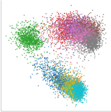
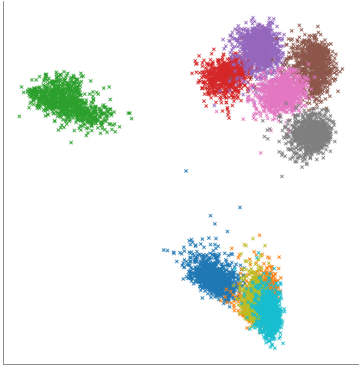
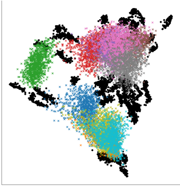
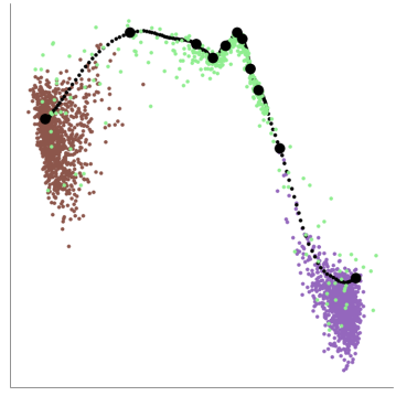
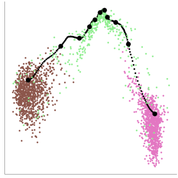
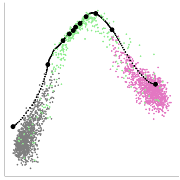
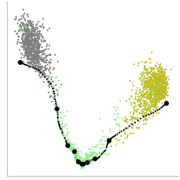
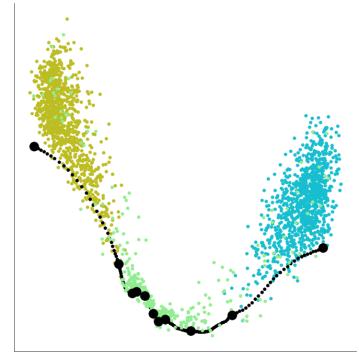
To ensure that the superposed latent embedding creates boundary supporting samples, we conducted an experiment to compare generated synthetic samples on feature space visually. The experimental results are based on the generators trained with ResNet-20 for CIFAR-10 dataset. The features were extracted from the intermediate activation before the last fully connected layer of the full-precision model. For the Qimera-based generator, we set K=2 during the sample generations for clarity.
After extracting the features, we projected the features into a two-dimensional space using Principal Component Analysis (PCA) [49]. The results are presented in Figure 3. Compared with the original training set data (Figure 3(a)), the samples from the GDFQ-based generator (Figure 3(b)) show a lack of boundary supporting samples and the class distributions are confined to small regions around the centroid of each class. A generator trained with Qimera, however, exhibits different characteristics (Figure 3(c)). Samples that are generated from superposed latent embeddings are displayed as black dots. The black dots are mostly located on the sparse regions between the class clusters. This experimental result shows that our method, Qimera, successfully generates samples near the decision boundaries. In other words, superposed latent embeddings are not only superposed on embedding space but also in the feature space, serving as synthetic boundary supporting samples.
5.3 Quantization Results Comparison
Table 2 displays the classification accuracy on various datasets, target models, and bit-width settings. Note that wa means -bit quantization for weights and -bit quantization for activations. As baselines, we selected ZeroQ [15], ZAQ [14], and GDFQ [13] as the important previous works on generative data-free quantization. In addition, we implemented Mixup [50] and Cutmix [51] on top of GDFQ, which are data augmentation schemes that mix input images. To implement these schemes, we created synthetic images from GDFQ, and applied the augmentations to build training images and labels. All baseline results are from official code of the authors, where a small amount of modifications have been made on the GDFQ baseline for applying Mixup and Cutmix. We report top-1 accuracy for each experiment. The numbers inside the parentheses of Qimera results are improvements over the highest baseline.
The results demonstrate that Qimera outperforms the baselines at almost all settings. Its performance improvement is especially large for low-bitwidth (4w4a) cases. For 5w5a setting, the gain is still significant, and its performance reaches near that of the full-precision model, which represents the upper bound. In addition, Qimera is not limited to small datasets having a low spatial dimension. The ImageNet results prove that Qimera performs beyond other baselines with considerable gaps, on a large-scale dataset with many classes. Interestingly, the result of GDFQ+Mixup and GDFQ+Cutmix did not produce much noticeable improvement except for GDFQ+Mixup in 4w4a ResNet -18 and -50. This implies that a mixture of generated synthetic samples of different classes in the sample space is not sufficient to represent boundary supporting samples. In summary, Qimera achieves superior accuracy on various environments regardless of dataset or model scale.
| Dataset | Model (FP32 Acc.) | Bits | ZeroQ | ZAQ | GDFQ | GDFQ +Cutmix | GDFQ +Mixup | Qimera (%p improvement) |
| Cifar-10 | ResNet-20 | 4w4a | 79.30 | 92.13∗ | 90.25 | 89.58 | 88.69 (-3.44) | 91.26 0.49 (-0.87) |
| (93.89) | 5w5a | 91.34 | 93.36 | 93.38∗ | 92.75 | 92.79 (-0.59) | 93.46 0.03 (+0.08) | |
| Cifar-100 | ResNet-20 | 4w4a | 47.45 | 60.42 | 63.39∗ | 62.74 | 62.99 (-0.40) | 65.10 0.33 (+1.71) |
| (70.33) | 5w5a | 65.61 | 68.70∗ | 66.12 | 67.51 | 67.78 (-0.92) | 69.02 0.22 (+0.32) | |
| ImageNet | ResNet-18 | 4w4a | 22.58 | 52.64 | 60.60∗ | 58.90 | 61.72 (+1.12) | 63.84 0.30 (+3.24) |
| (71.47) | 5w5a | 59.26 | 64.54 | 68.40∗ | 68.05 | 68.67 (+0.27) | 69.29 0.16 (+0.89) | |
| ResNet-50 | 4w4a | 08.38 | 53.02∗ | 52.12 | 51.80 | 59.25 (+6.24) | 66.25 0.90 (+13.23) | |
| (77.73) | 5w5a | 48.12 | 73.38∗ | 71.89 | 70.99 | 71.57 (-1.81) | 75.32 0.09 (+1.94) | |
| MobileNetV2 | 4w4a | 10.96 | 00.10† | 59.43∗ | 57.23 | 59.99 (+0.56) | 61.62 0.39 (+2.19) | |
| (73.03) | 5w5a | 59.88 | 62.35 | 68.11∗ | 67.61 | 68.83 (+0.72) | 70.45 0.07 (+2.34) | |
| ∗ Highest among the baselines †Did not converge | ||||||||
5.4 Qimera on Top of Various Algorithms
| Dataset | Model (FP32 Acc.) | Bits | GDFQ | Qimera + GDFQ | ZAQ | Qimera + ZAQ | AutoReCon | Qimera + AutoReCon |
| Cifar-10 | ResNet-20 | 4w4a | 90.25 | 91.26 (1.01) | 92.13 | 93.91 (1.78) | 88.55 | 91.16 (2.61) |
| (93.89) | 5w5a | 93.38 | 93.46 (0.08) | 93.36 | 93.84 (0.48) | 92.88 | 93.42 (0.54) | |
| Cifar-100 | ResNet-20 | 4w4a | 63.39 | 65.10 (1.71) | 60.42 | 69.30 (8.88) | 62.76 | 65.33 (2.57) |
| (70.33) | 5w5a | 66.12 | 69.02 (2.90) | 68.70 | 69.58 (0.88) | 68.40 | 68.80 (0.40) |
In this paper, we have applied GDFQ [13] as a baseline. However, our design does not particularly depend on a certain method, and can be adopted by many schemes. To demonstrate this, we implemented Qimera on top of ZAQ [14] and AutoReCon [27]. The results are shown in Table 3.
AutoReCon [27] strengthens the generator architecture using a neural architecture search, and therefore applying this is no different from that of the original Qimera implemented on top of GDFQ. However, original ZAQ does not use per-class sample generation. To attach the techniques from Qimera, we extended the generator with an embedding layer, and added a cross-entropy loss into the loss function as the following:
| (11) |
| (12) |
where was set to 0.1, and , are calculated based on Eq. 8.
For all cases, applying the techniques of Qimera improves the performance by a significant amount. Especially for Qimera + ZAQ, the performances obtained was better than those of our primary implementation Qimera + GDFQ. Unfortunately, it did not converge with ImageNet, and thus we did not consider this implementation as the primary version of Qimera.
5.5 Further Experiments
We discuss some aspects of our method in this section, which are effect of each scheme introduced in Section 4 on the accuracy of , a sensitivity study upon various and settings, and a closer investigation into the effect of disentanglement mapping (DM) and extracted embedding initialization (EEI) on the embedding space. All experiments in this subsection are under 4w4a setting.
Ablation study. We conducted an ablation study by adding the proposed components one by one on the GDFQ baseline. The results are presented in Table 4. As we can see, the superposed embedding (SE) alone brings a substantial amount of performance improvement for both Cifar-100 (1.16%p) and ImageNet (11.98%p). On Cifar-100, addition of EEI provides much additional gain of 0.68%p, while that of DM is marginal. ImageNet, on the other hand, DM provides 1.97%p additional gain, much larger than that of EEI. When both of DM and EEI are used together with SE, the additional improvement over the best among (+SE, DM) and (+SE, EEI) is relatively small. We believe this is because DM and EEI serve for the similar purposes. However, applying both techniques can achieve near-best performance regardless of the dataset.
Sensitivity Analysis. Table 4 also provides a sensitivity analysis for (number of classes for superposed embeddings) and (ratio of synthetic boundary supporting samples within the dataset). As shown in the table, both parameter clearly have an impact on the performance. For Cifar-100, the sweet spot values for and are both small, while those of the ImageNet were both large. We believe is because ImageNet has more classes. Because the number of class pairs (and the decision boundaries) is a quadratic function of number of classes, there needs more boundary supporting samples with more embeddings superposed to draw the correct border.
| Dataset | Method | Best | |||||||||
| 0.4 | 0.7 | 0.4 | 0.7 | 0.4 | 0.7 | 0.4 | 0.7 | ||||
| Cifar-100 | Baseline | N/A | N/A | N/A | N/A | N/A | N/A | N/A | N/A | 63.39 | |
| (ResNet-20) | +SE1 | 64.14 | 64.55 | 64.55 | 64.37 | 64.21 | 64.11 | 63.77 | 64.26 | 64.55 (+1.16) | |
| +SE, DM2 | 64.73 | 64.76 | 64.01 | 64.22 | 63.60 | 64.32 | 63.82 | 64.63 | 64.76 (+1.37) | ||
| +SE, EEI3 | 64.64 | 64.54 | 64.89 | 64.83 | 65.23 | 64.33 | 64.88 | 64.70 | 65.23 (+1.84) | ||
| +SE, DM, EEI | 64.90 | 64.76 | 65.10 | 64.52 | 64.72 | 64.4 | 64.63 | 64.79 | 65.10 (+1.71) | ||
| Dataset | Method | Best | |||||||||
| 0.4 | 0.7 | 0.4 | 0.7 | 0.4 | 0.7 | 0.4 | 0.7 | ||||
| ImageNet | Baseline | N/A | N/A | N/A | N/A | N/A | N/A | N/A | N/A | 52.12 | |
| (ResNet-50) | +SE | 57.34 | 60.93 | 59.27 | 62.91 | 63.12 | 64.09 | 61.04 | 60.89 | 64.09 (+11.98) | |
| +SE, DM | 59.59 | 64.12 | 63.97 | 64.87 | 62.16 | 64.72 | 65.43 | 66.06 | 66.06 (+13.94) | ||
| +SE, EEI | 56.52 | 62.23 | 61.24 | 61.08 | 54.45 | 62.87 | 54.84 | 64.44 | 64.44 (+12.32) | ||
| +SE, DM, EEI | 61.43 | 63.87 | 62.16 | 64.5 | 59.82 | 66.25 | 59.18 | 65.12 | 66.25 (+14.13) | ||
| 1Superposed Embeddings 2Disentanglement Mapping 3Extracted Embedding Initialization | |||||||||||
| Method | Cifar-10 | Cifar-100 | ||
| Dist. Ratio | Intrusion | Dist. Ratio | Intrusion | |
| Mixup | 2.44 | 0.800 | 3.14 | 0.400 |
| SE Only | 1.58 | 0.00260 | 1.64 | 0.053 |
| SE+DM | 1.67 | 0.00073 | 1.59 | 0.044 |
| SE+DM+EEI | 1.57 | 0.00013 | 1.52 | 0.029 |
Investigation into the Embedding Space. To investigate how DM and EEI help shaping the embedding space friendly to SE, we conducted two additional experiments with ResNet-20 in Table 5. First, setting =2 (between two classes), we measured the ratio of the perceptual distance and Euclidean distance between the two embeddings in the classifier’s feature space. The perceptual distance is measured by sweeping from Eqs. 6 and 7 from 0 to 1 by 0.01 and adding all the piecewise distances between points in the feature space (See Figure 5 in Appendix). We want the distance ratio to be close to 1.0 for the embedding space distribution to be similar to that of the feature space. Second, we defined ‘intrusion score’, the sum of logits that are outside the chosen pair of classes. If the score is large, that means the synthetic boundary samples are regarded as samples of non-related classes. Therefore, lower scores are desired. For comparison, we have also included the Mixup as a naive method and measured both metrics. It shows that the DM and EEI are effective for in terms of both the distance ratio and the intrusion score, explaining how DM and EEI achieves better performances.
6 Discussion
6.1 Does it Cause Invasion of Privacy?
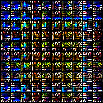
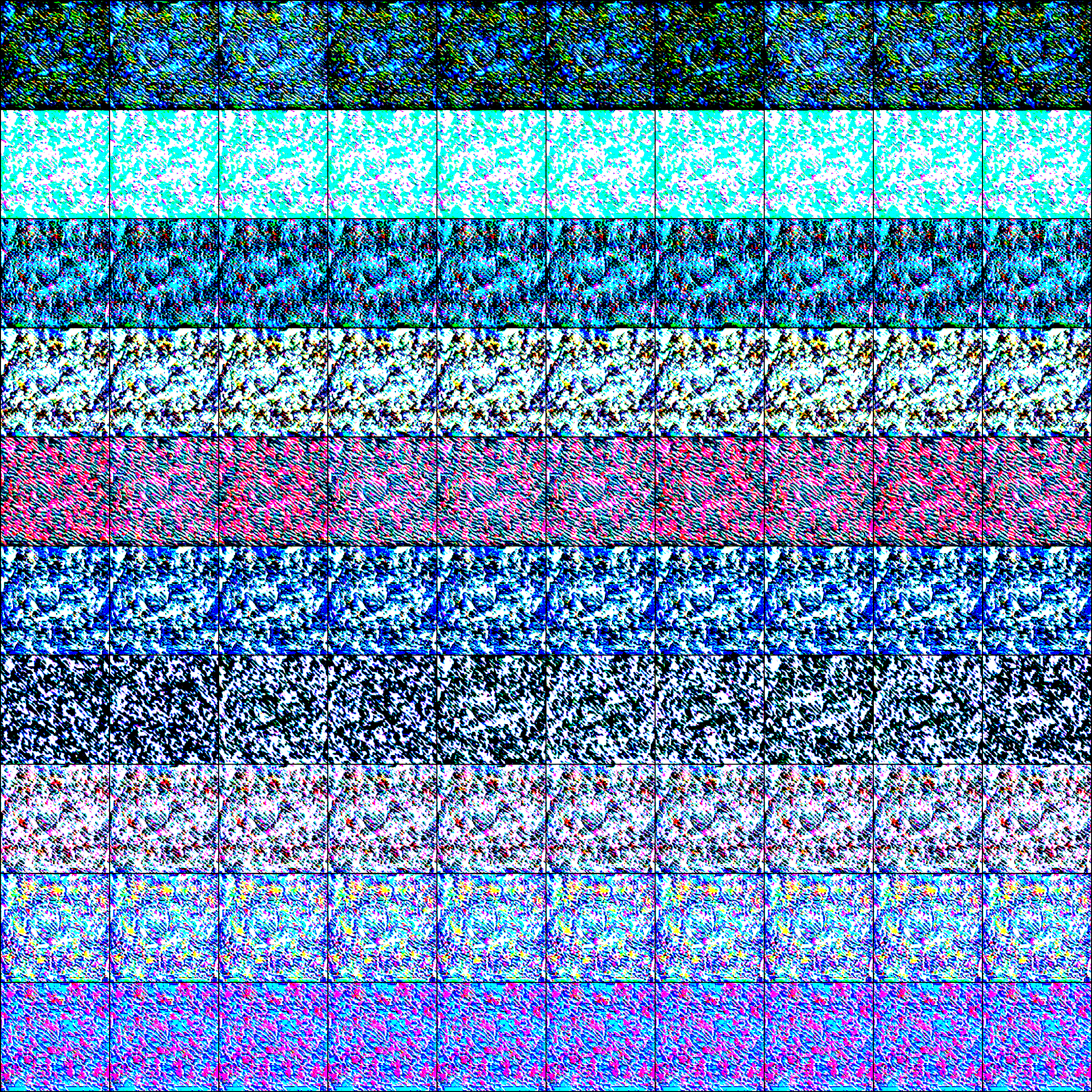
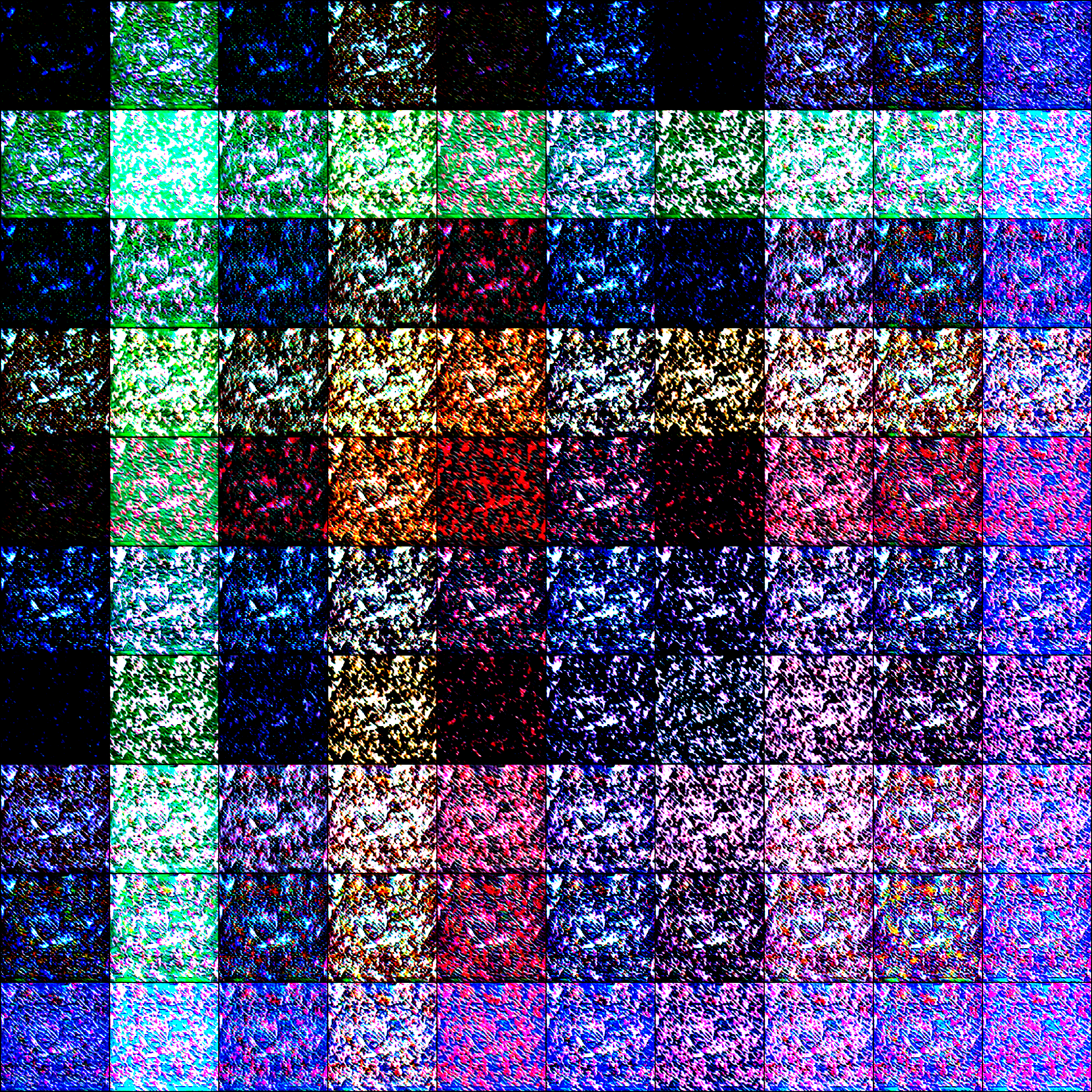
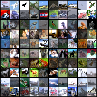
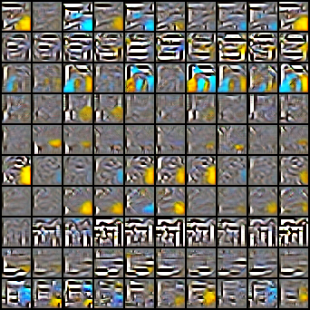
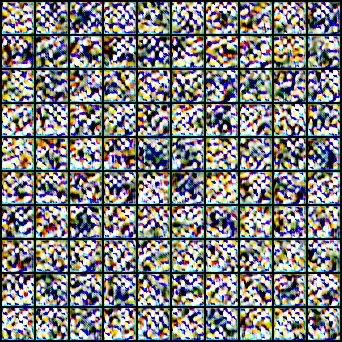
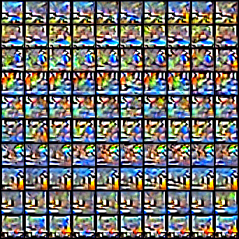
The motivation for data-free quantization is that the private original data might not be available. Using a generator to reconstruct samples that follow the distribution of original data might indicate the invasion of privacy. However, as displayed in Figure 4, at least with current technologies, there is no sign of privacy invasion. The generated data are far from being human interpretable, which was also the case for previous works [15, 14, 13]. See Appendix (Figure 6) for more generated images.
Geirhos et al. [52] reveal an interesting property that CNNs are heavily biased by local textures, not global shapes. BagNet [53] supports this claim by confirming that images with distorted shapes but preserved textures can still mostly be correctly classified by CNNs. In such regard, it is no wonder that the generated samples are non-interpretable, because there is only a few combinations that maintains the global shape out of all possibilities that preserve the textures. Nonetheless, not being observed does not guarantee the privacy protection. We believe it is a subject for further investigations.
6.2 Limitations
Even though Qimera achieves a superior performance, one drawback of this approach is the fact that it utilizes embeddings of multiple classes to generate the boundary supporting samples. This restricts its application to classification tasks and its variants. For example, generation of datasets such as image segmentation or object detection do not take class embeddings as the input. However, generators for such data are not extensively studied yet, and we envision adding diversity to them would require inputting some form of labels or embeddings similar to paint-to-image [54], which would allow Qimera be easily applied.
7 Conclusion
In this paper, we have proposed Qimera, a simple yet powerful approach for data-free quantization by generating synthetic boundary supporting samples with superposed latent embeddings. We show in our motivational experiment that current state-of-the-art generative data-free quantization can be greatly improved by a small set of boundary supporting samples. Then, we show that superposing latent embeddings can close much of the gap. Extensive experimental results on various environments shows that Qimera achieves state-of-the-art performance for many networks and datasets, especially for large-scale datasets.
Acknowledgments and Disclosure of Funding
This work was supported by National Research Foundation of Korea (NRF) grant funded by the Korea government(MSIT) (No.2021R1F1A1063670, No.2020R1F1A1074472) and Institute of Information & communications Technology Planning & Evaluation (IITP) grant funded by the Korea government (MSIT) (No.2020-0-01361, Artificial Intelligence Graduate School Program (Yonsei University))
References
- [1] Norman P Jouppi et al. “In-datacenter performance analysis of a tensor processing unit” In Proceedings of the International Symposium on Computer Architecture, 2017
- [2] Song Han, Huizi Mao and William J Dally “Deep compression: Compressing deep neural networks with pruning, trained quantization and huffman coding” In International Conference on Learning Representations, 2016
- [3] Geoffrey Hinton, Oriol Vinyals and Jeff Dean “Distilling the knowledge in a neural network” In Advances in Neural Information Processing Systems Workshops, 2014
- [4] Shuchang Zhou et al. “Dorefa-net: Training low bitwidth convolutional neural networks with low bitwidth gradients” In arXiv preprint arXiv:1606.06160, 2016
- [5] Bohan Zhuang et al. “Towards effective low-bitwidth convolutional neural networks” In Proceedings of the IEEE/CVF Conference on Computer Vision and Pattern Recognition, 2018
- [6] Chuang Gan Lin and Song Han “Defensive quantization: When efficiency meets robustness” In International Conference on Learning Representations, 2018
- [7] Benoit Jacob et al. “Quantization and training of neural networks for efficient integer-arithmetic-only inference” In Proceedings of the IEEE/CVF Conference on Computer Vision and Pattern Recognition, 2018
- [8] Sheng Shen et al. “Q-BERT: Hessian based ultra low precision quantization of BERT” In Proceedings of the AAAI Conference on Artificial Intelligence, 2020
- [9] Ron Banner, Yury Nahshan, Elad Hoffer and Daniel Soudry “Post-training 4-bit quantization of convolution networks for rapid-deployment” In arXiv preprint arXiv:1810.05723, 2018
- [10] Markus Nagel, Mart van Baalen, Tijmen Blankevoort and Max Welling “Data-free quantization through weight equalization and bias correction” In Proceedings of the IEEE/CVF International Conference on Computer Vision, 2019
- [11] Yoojin Choi, Jihwan Choi, Mostafa El-Khamy and Jungwon Lee “Data-free network quantization with adversarial knowledge distillation” In Proceedings of the IEEE/CVF Conference on Computer Vision and Pattern Recognition Workshops, 2020
- [12] Ritchie Zhao et al. “Improving neural network quantization without retraining using outlier channel splitting” In International Conference on Machine Learning, 2019
- [13] Shoukai Xu et al. “Generative low-bitwidth data free quantization” In European Conference on Computer Vision, 2020
- [14] Yuang Liu, Wei Zhang and Jun Wang “Zero-shot adversarial quantization” In arXiv preprint arXiv:2103.15263, 2021
- [15] Yaohui Cai et al. “ZeroQ: A novel zero shot quantization framework” In Proceedings of the IEEE/CVF Conference on Computer Vision and Pattern Recognition, 2020
- [16] Byeongho Heo, Minsik Lee, Sangdoo Yun and Jin Young Choi “Knowledge distillation with adversarial samples supporting decision boundary” In Proceedings of the AAAI Conference on Artificial Intelligence, 2019
- [17] Mehdi Mirza and Simon Osindero “Conditional generative adversarial nets” In Advances in Neural Information Processing Systems Workshops, 2014
- [18] Augustus Odena, Christopher Olah and Jonathon Shlens “Conditional image synthesis with auxiliary classifier gans” In International Conference on Machine Learning, 2017
- [19] Raphael Gontijo Lopes, Stefano Fenu and Thad Starner “Data-free knowledge distillation for deep neural networks” In arXiv preprint arXiv:1710.07535, 2017
- [20] Gaurav Kumar Nayak et al. “Zero-shot knowledge distillation in deep networks” In International Conference on Machine Learning, 2019
- [21] Ian J Goodfellow et al. “Generative adversarial nets” In Advances in Neural Information Processing Systems, 2014
- [22] Hanting Chen et al. “Data-free learning of student networks” In Proceedings of the IEEE/CVF International Conference on Computer Vision, 2019
- [23] Paul Micaelli and Amos Storkey “Zero-shot knowledge transfer via adversarial belief matching” In arXiv preprint arXiv:1905.09768, 2019
- [24] Gongfan Fang et al. “Data-free adversarial distillation” In arXiv preprint arXiv:1912.11006, 2019
- [25] Hongxu Yin et al. “Dreaming to distill: Data-free knowledge transfer via deepinversion” In Proceedings of the IEEE/CVF Conference on Computer Vision and Pattern Recognition, 2020
- [26] Jaemin Yoo, Minyong Cho, Taebum Kim and U Kang “Knowledge extraction with no observable data” In Advances in Neural Information Processing Systems, 2019
- [27] Baozhou Zhu et al. “AutoReCon: Neural Architecture Search-based Reconstruction for Data-free Compression” In arXiv preprint arXiv:2105.12151, 2021
- [28] Xiangguo Zhang et al. “Diversifying Sample Generation for Accurate Data-Free Quantization” In Proceedings of the IEEE/CVF Conference on Computer Vision and Pattern Recognition, 2021, pp. 15658–15667
- [29] Hongyu Guo, Yongyi Mao and Richong Zhang “Mixup as locally linear out-of-manifold regularization” In Proceedings of the AAAI Conference on Artificial Intelligence, 2019
- [30] Christian Szegedy et al. “Intriguing properties of neural networks” In International Conference on Learning Representations, 2014
- [31] Zihe Dong, Xin Sun, Junyu Dong and Haoran Zhao “Adversarial metric knowledge distillation” In International Conference on Communication and Information Processing, 2020
- [32] Hamid Karimi, Tyler Derr and Jiliang Tang “Characterizing the decision boundary of deep neural networks” In arXiv preprint arXiv:1912.11460, 2019
- [33] Kuniaki Saito, Donghyun Kim, Stan Sclaroff and Kate Saenko “Universal Domain Adaptation through Self Supervision” In Advances in Neural Information Processing Systems, 2020
- [34] Yujie Xu, Xiaowei Qin, Xiaodong Xu and Jianqiang Chen “Open-set interference signal recognition using boundary samples: A hybrid approach” In International Conference on Wireless Communications and Signal Processing, 2020
- [35] Alex Krizhevsky and Geoffrey Hinton “Learning multiple layers of features from tiny images” Citeseer, 2009 URL: http://www.cs.utoronto.ca/~kriz/learning-features-2009-TR.pdf
- [36] Kaiming He, Xiangyu Zhang, Shaoqing Ren and Jian Sun “Deep residual learning for image recognition” In Proceedings of the IEEE conference on Computer Vision and Pattern Recognition, 2016
- [37] Tero Karras, Samuli Laine and Timo Aila “A style-based generator architecture for generative adversarial networks” In Proceedings of the IEEE/CVF Conference on Computer Vision and Pattern Recognition, 2019
- [38] Georgios Arvanitidis, Lars Kai Hansen and Søren Hauberg “Latent space oddity: On the curvature of deep generative models” In International Conference on Learning Representations, 2018
- [39] Samuli Laine “Feature-based metrics for exploring the latent space of generative models” In International Conference on Learning Representations Workshops, 2018
- [40] Kuniaki Saito et al. “Semi-supervised domain adaptation via minimax entropy” In Proceedings of the IEEE/CVF International Conference on Computer Vision, 2019
- [41] Alex Krizhevsky, Ilya Sutskever and Geoffrey E Hinton “Imagenet classification with deep convolutional neural networks” In Advances in Neural Information Processing Systems, 2012
- [42] Mark Sandler et al. “Mobilenetv2: Inverted residuals and linear bottlenecks” In Proceedings of the IEEE/CVF Conference on Computer Vision and Pattern Recognition, 2018
- [43] Adam Paszke et al. “Automatic differentiation in pytorch” In Advances in Neural Information Processing Systems Workshops, 2017
- [44] “Computer vision models on PyTorch” URL: https://pypi.org/project/pytorchcv/
- [45] Diederik P. Kingma and Jimmy Ba “Adam: A Method for Stochastic Optimization” In International Conference for Learning Representations, 2015
- [46] Harm Vries et al. “Modulating early visual processing by language” In Advances in Neural Information Processing Systems, 2017
- [47] Takeru Miyato, Toshiki Kataoka, Masanori Koyama and Yuichi Yoshida “Spectral Normalization for Generative Adversarial Networks” In arXiv preprint arXiv:1802.05957, 2018
- [48] Y. E. Nesterov “A method for solving the convex programming problem with convergence rate ” In Dokl. Akad. Nauk SSSR, 1983
- [49] Karl Pearson F.R.S. “LIII. On lines and planes of closest fit to systems of points in space” In The London, Edinburgh, and Dublin Philosophical Magazine and Journal of Science Taylor & Francis, 1901
- [50] Hongyi Zhang, Moustapha Cisse, Yann N Dauphin and David Lopez-Paz “Mixup: Beyond empirical risk minimization” In Internation Conference on Learning Representations, 2018
- [51] Sangdoo Yun et al. “Cutmix: Regularization strategy to train strong classifiers with localizable features” In Proceedings of the IEEE/CVF International Conference on Computer Vision, 2019
- [52] Robert Geirhos et al. “ImageNet-trained CNNs are biased towards texture; increasing shape bias improves accuracy and robustness” In International Conference on Learning Representations, 2018
- [53] Wieland Brendel and Matthias Bethge “Approximating CNNs with Bag-of-local-Features models works surprisingly well on ImageNet” In International Conference on Learning Representations, 2018
- [54] Tamar Rott Shaham, Tali Dekel and Tomer Michaeli “SinGAN: Learning a generative model from a single natural image” In Proceedings of the IEEE/CVF International Conference on Computer Vision, 2019
Appendix A Code
The whole code is available at https://github.com/iamkanghyunchoi/qimera, including the training, evaluation, and visualization for all settings. This project code is licensed under the terms of the GNU General Public License v3.0.
Appendix B Additional Experimental Results
B.1 Baseline with Different Noise Level
Instead of the superposed embeddings, we tried the alternative of adjusting the variance of the noise inputs, as discussed in Section 4.1 of the main body. We have tested five values as standard deviation : 0.25, 0.5, 1.0, 1.5, and 2.0. The results in Table 6 show that as we hypothesized, just by increasing the noise level did not provide much improvement on the performance of the baseline. Instead, we have noticed a slight improvement on GDFQ when the noise level is decreased, and we believe this is due to the generation of clearer samples. Nonetheless, the accuracy is far below that of the proposed Qimera.
| Dataset | Model | Bits | GDFQ | Qimera | ||||||
| 0.25 | 0.50 | 1.0* | 1.5 | 2.0 | ||||||
| Cifar-10 | ResNet-20 | 4w4a | 90.82 | 90.59 | 90.25 | 90.10 | 89.99 | 91.26 | ||
| 5w5a | 93.45 | 93.45 | 93.38 | 93.30 | 93.31 | 93.46 | ||||
| Cifar-100 | ResNet-20 | 4w4a | 64.33 | 63.70 | 63.39 | 63.47 | 63.18 | 65.10 | ||
| 5w5a | 68.17 | 68.37 | 66.12 | 67.46 | 67.33 | 69.02 | ||||
| ImageNet | ResNet-18 | 4w4a | 61.47 | 60.91 | 60.60 | 60.25 | 60.20 | 63.84 | ||
| 5w5a | 68.92 | 68.25 | 68.40 | 68.37 | 68.07 | 69.29 | ||||
| ResNet-50 | 4w4a | 55.30 | 54.37 | 52.12 | 54.29 | 46.14 | 66.25 | |||
| 5w5a | 72.01 | 72.56 | 71.89 | 71.60 | 71.14 | 75.32 | ||||
| MobileNetV2 | 4w4a | 60.29 | 59.90 | 59.43 | 58.67 | 59.31 | 61.62 | |||
| 5w5a | 68.69 | 68.35 | 68.11 | 68.10 | 67.84 | 70.45 | ||||
| *Default value from | ||||||||||
B.2 Extracted Embedding Initialization without Training
| Dataset | Model (FP32 Acc.) | Bits | ZeroQ | ZAQ | GDFQ | Qimera | Extracted Init + Freeze |
| Cifar-10 | ResNet-20 | 4w4a | 79.30 | 92.13∗ | 90.25 | 91.26 | 90.37 |
| (93.89) | 5w5a | 91.34 | 93.36 | 93.38∗ | 93.46 | 93.25 | |
| Cifar-100 | ResNet-20 | 4w4a | 47.45 | 60.42 | 63.39∗ | 65.10 | 63.83 |
| (70.33) | 5w5a | 65.61 | 68.70∗ | 66.12 | 69.02 | 68.76 | |
| ImageNet | ResNet-18 | 4w4a | 22.58 | 52.64 | 60.60∗ | 63.84 | 63.67 |
| (71.47) | 5w5a | 59.26 | 64.54 | 68.40∗ | 69.29 | 69.23 | |
| ResNet-50 | 4w4a | 08.38 | 53.02∗ | 52.12 | 66.25 | 63.20 | |
| (77.73) | 5w5a | 48.12 | 73.38∗ | 71.89 | 75.32 | 74.84 | |
| MobileNetV2 | 4w4a | 10.96 | 00.10† | 59.43∗ | 61.62 | 60.46 | |
| (73.03) | 5w5a | 59.88 | 62.35 | 68.11∗ | 70.45 | 68.82 | |
| ∗ Highest among the baselines †Did not converge | |||||||
To show that the weight from the last fully connected layer of the full-precision model is a good candidate for the initial embeddings, we have performed an experiment where the embeddings are frozen right after initialization. The results are presented in Table 7. Qimera with frozen embeddings are not better than the primary Qimera method with trained embeddings. However, compared to the two baselines (ZAQ and GDFQ), they provides a comparable accuracy on Cifar-10 and better accuracies on Cifar-100 and ImageNet. Furthermore, the accuracy on Cifar-10 dataset is close to the upper bound for all techniques under comparison, and thus the differences are minimal.
B.3 Sensitivity Study on Number of DM layers
| Num. DM Layers | Accuracy | |
| Cifar-10 | Cifar-100 | |
| (w/o DM) | 90.81 | 64.89 |
| 1 | 91.26 | 65.10 |
| 2 | 91.18 | 64.90 |
| 4 | 91.49 | 64.96 |
| 8 | 91.63 | 64.11 |
To have a deeper look into the DM layers, we have conducted a sensitivity study on the number of DM layers in Table 8. In the table, all results are from 4w4a setting with =0.4, =2 for Cifar-10 and =10 for Cifar-100. As displayed, we found that there are sometimes small improvements from using more DM layers above one, but a severe drop in performance has been observed for using too many layers (Cifar-100, 8 layers).
B.4 More Sensitivity Study on Hyperparameters
| Dataset | |||||||
| 0.10 | 0.25 | 0.40 | 0.55 | 0.70 | 0.85 | ||
| Cifar-100 (ResNet-20) | 2 | 64.18 | 64.62 | 64.90 | 64.95 | 64.76 | 64.89 |
| 10 | 64.85 | 64.63 | 65.10 | 64.76 | 64.52 | 63.86 | |
| 25 | 64.53 | 64.91 | 64.72 | 64.66 | 64.40 | 64.01 | |
| 100 | 64.37 | 64.66 | 64.64 | 64.27 | 64.79 | 63.65 | |
| ImageNet (ResNet-50) | 100 | 58.74 | 60.64 | 61.43 | 61.47 | 63.87 | 65.73 |
| 250 | 61.30 | 61.28 | 62.16 | 64.03 | 64.50 | 65.23 | |
| 500 | 58.96 | 60.11 | 58.69 | 63.05 | 66.25 | 66.19 | |
| 1000 | 58.65 | 59.62 | 61.20 | 58.86 | 65.12 | 64.24 | |
In addition to our choice of hyperparameters presented in the main body, we have performed a further extensive sensitivity study on those parameters, which is displayed in Table 9. All experiments are against 4w4a configuration, equal to the Table 3 (Section 5.4) in the main body. Regardless of the choice in and , the results are all better than the two baselines ZAQ and GDFQ. Furthermore, while they all provide a meaningfully good performance, the results show a clear trend: lower for Cifar-10/100 and higher for ImageNet as sweet spots. This result supports the use of Qimera in that these parameters are easily tunable, not something that must be exhaustively seAutoReConhed for optimal values.
B.5 Comparison with DSG
| Dataset | Model | Bits | DSG [28] | Qimera (%p improvement) |
| ImageNet | ResNet-18 | 4w4a | 34.53 | 63.84 (+29.31) |
| ResNet-50 | 6w6a | 76.07 | 77.18 (+1.11) | |
| InceptionV3 | 4w4a | 34.89 | 73.31 (+38.42) | |
| SqueezeNext | 6w6a | 60.50 | 65.97 (+5.47) | |
| ShuffleNet | 6w6a | 44.88 | 56.16 (+11.28) |
Qimera is conceptually similar to DSG [28] which tries to diversify the sample generation by relaxing the batch-norm stat alignments. However, Qimera is different from DSG because we explicitly try to generate boundary supporting samples, instead of relying on diversification. This would led to better performance as demonstrated in the motivational experiment of Section 3.
Table 10 shows the comparison of Qimera with DSG. We use the reported numbers for DSG, and perform a new set of experiments for Qimera to match the settings. We use the lowest-bit settings for each network evaluated in DSG. As displayed in the table, Qimera outperforms DSG in all settings, especially for 4w4a cases.
Appendix C Class-Pairwise Visualization
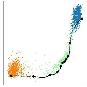
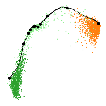
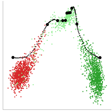
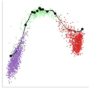
To look closely onto the visualization of the samples from Section 5.3 (Figure 3) in the main body, we have plotted them in a pair-wise manner. Even though 10 classes in total gives 45 possible pairs, we chose nine symbolically adjacent pairs in the figure. Although being symbolically adjacent does not have much meaning, we believe having nine pairs is enough for our purpose rather than showing all 45 possible pairs. The colors match that of the Figure 3, where the lightgreen dots represent the synthetic boundary supporting samples. Also, we have plotted the path between the centroids of the two clusters in black, by varying (the ratio of superposition) from 0 to 1 by 0.01 without any noise. Each 10th percentile is denoted as larger black dots. The results show that the samples and the path lie relatively in the middle of the two clusters. Please note that we have performed PCA plot for each pair to best show the distribution, so the position and orientation of the clusters do not exactly match those from Figure 3.
Appendix D More Generated Images
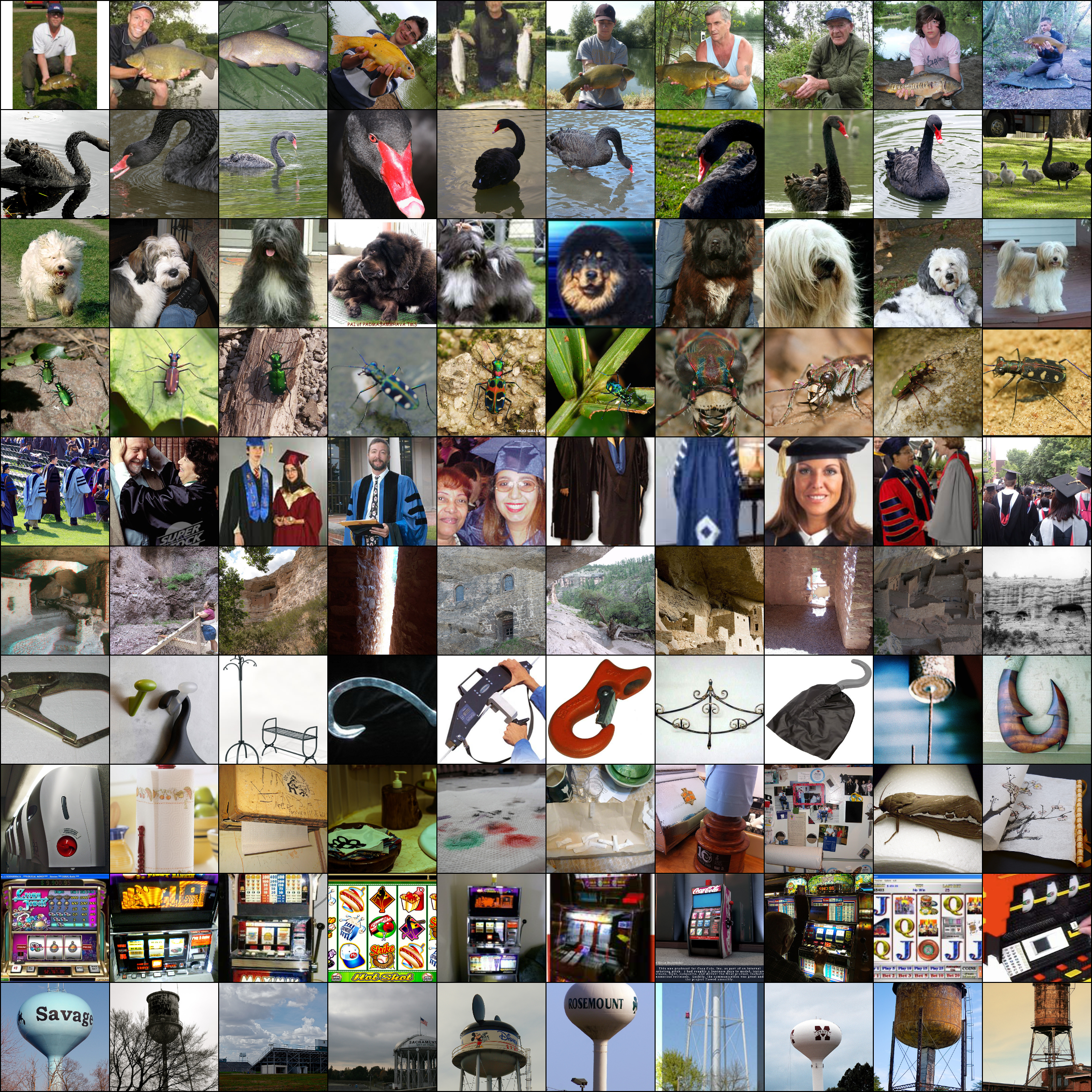
Lastly, Figure 6 shows more samples generated from Qimera. Figure 6(a) displays the synthetic boundary supporting samples generated from Cifar-10 dataset, with and . Each row and column represents a class from Cifar-10. For example, the image at row 0 (airplane) and column 2 (bird) represents a sample generated from superposed embeddings of airplane and bird. Although still not very human-recognizable, we find that each sample in Figure 6(a) has some features adopted from each of the source classes in Figure 4d.
Figure 6(c) shows the sample images created from ImageNet. Because there are too many classes within ImageNet (1000), we chose 10 classes from them, which are {0: ‘tench, Tinca tinca’, 100: ‘black swan, Cygnus atratus’, 200: ‘Tibetan terrier, chrysanthemum dog’, 300: ‘tiger beetle’, 400: ‘academic gown, academic robe, judge’s robe", 500: ‘cliff dwelling’, 600: ‘hook, claw’, 700: ‘paper towel’, 800: ‘slot, one-armed bandit’, 900: ‘water tower’}, and the original samples from those classes are shown in Figure 6(b). As in Cifar-10, the generated samples are far from human-recognizable, but each row is clearly distinguishable from the others. In addition, Figure 6(d) contains the synthetic boundary supporting samples from ImageNet, following the same rules from Figure 6(a). Again, we see that each position in the sample matrix adopts features from the rows of the corresponding class pair in Figure 6(c).