Realtime Trajectory Smoothing with Neural Nets

Abstract

In order to safely and efficiently collaborate with humans, industrial robots need the ability to alter their motions quickly to react to sudden changes in the environment, such as an obstacle appearing across a planned trajectory. In Realtime Motion Planning, obstacles are detected in real time through a vision system, and new trajectories are planned with respect to the current positions of the obstacles, and immediately executed on the robot. Existing realtime motion planners, however, lack the smoothing post-processing step – which are crucial in sampling-based motion planning – resulting in the planned trajectories being jerky, and therefore inefficient and less human-friendly. Here we propose a Realtime Trajectory Smoother based on the shortcutting technique to address this issue. Leveraging fast clearance inference by a novel neural network, the proposed method is able to consistently smooth the trajectories of a 6-DOF industrial robot arm within 200 ms on a commercial GPU. We integrate the proposed smoother into a full Vision–Motion Planning–Execution loop and demonstrate a realtime, smooth, performance of an industrial robot subject to dynamic obstacles.

I Introduction

In order to safely and efficiently collaborate with humans, robots need the ability to alter their motions quickly to react to sudden changes in the environment, such as an obstacle appearing across a planned trajectory. In most industrial applications, one would stop the robot upon the detection of obstacles in the robot’s reach space. However, such a solution is inefficient and precludes true human-robot collaboration, where humans and robots are to share a common workspace.

Recently, Realtime Motion Planning (RMP) has been proposed to enable true human-robot collaboration: obstacles are detected in real time through a vision system, new trajectories are planned with respect to the current positions of the obstacles, and immediately executed on the robot. RMP requires extremely fast computation in the Vision–Motion Planning–Execution loop. In particular, several techniques have been proposed for the Motion Planning component, relying on the parallelization of sampling-based algorithms [1, 2] on dedicated hardware, such as GPU [3, 4] or FPGA [5].

Sampling-based motion planners typically output jerky trajectories and therefore almost always require a smoothing post-processing step (see e.g. [6] for a detailed review). To our knowledge, existing realtime motion planners lack this step , presumably because of the large computation time associated with trajectory smoothing. Indeed, to obtain an acceptable trajectory quality, smoothing time is comparable, if not longer than initial path planning time [6]. As a result, while the motions produced by Realtime Motion Planning enable safely adapting to sudden changes in the environment, the lack of smoothness makes them inefficient and less human-friendly. In the particular context of human-robot collaboration, smooth trajectories indeed appear more predictable and agreeable to humans (see e.g. [7] for a discussion).

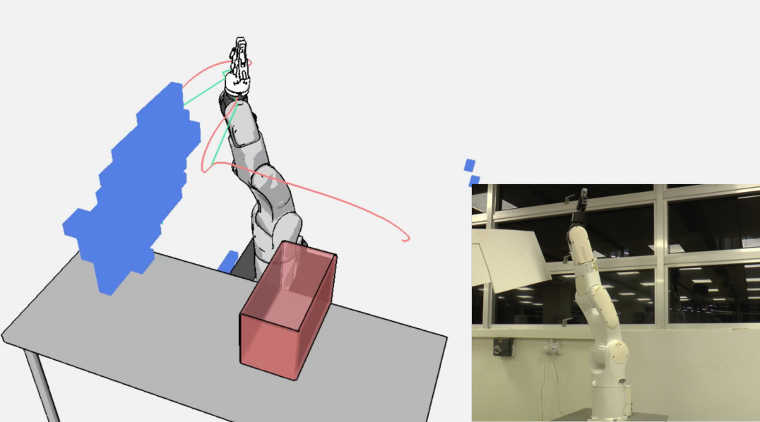
Figure 1: A robot avoids a dynamic obstacle by realtime trajectory re-planning and smoothing with the proposed smoother. Green: jerky trajectory planned by realtime PRM. Red: trajectory after smoothing. See the video of the experiment at  %****␣sample.tex␣Line␣175␣****https://youtu.be/XQFEmFyUaj8.

Here we propose a Realtime Trajectory Smoother based on the shortcutting technique [8, 9] to address this issue. Leveraging fast clearance inference by a novel neural network, the proposed method is able to consistently smooth the trajectories of a 6-DOF industrial robot arm within 200 ms on a commercial GPU, which is 2 to 3 times faster than state-of-the-art smoothers. Combined with even rudimentary, in-house, implementations of a vision pipeline and a sampling-based motion planner, we were able to achieve 300 ms cycle time, which is sufficient for realtime performance (Fig. 1). Note again here that smoothing is indeed the bottleneck, as the initial planning time was only $\sim 40$ ms.

The paper is organized as follows. We survey related work on obstacle avoidance and collision estimation in Section II. In Section III, we present our trajectory smoothing pipeline and the structure of the neural network model for fast clearance inference. In Section IV, we evaluate the pipeline in two sets of experiments. First, we evaluate the clearance inference accuracy of the neural network. Second, we integrate the smoother into a full-fledged Vision–Planning–Execution loop, and demonstrate a realtime, smooth, performance of a physical industrial robot subject to dynamic obstacles. Finally, we discuss the advantages and limitations of our approach and conclude with some directions for future work (Section V).

II Related Work

In this section, we give a brief overview of prior work on realtime motion planning in dynamic environments, trajectory smoothing, optimization-based planning and reactive control.

II-A Realtime Motion Planning

The major sampling-based planners are Rapidly-exploring Random Tree (RRT)[1] and Probabilistic Roadmaps (PRM)[2], and both have realtime versions. RT-RRT* is a tree rewiring technique for RRT which keeps removing nodes and edges colliding with dynamic obstacles and adding new nodes and edges[10]. g-Planner is an RRT-based technique to utilize GPU’s parallel computation mechanism to accelerate configuration node sampling and collision checking[3, 4]. Parallel Poisson RRT also exploits GPU for tree expansion, nearest neighbor search, and collision checking[11]. On the other hand, Murray et al. [5] use FPGA for a PRM-based planner by voxelizing the environment and caching collision information into each edge of PRM’s roadmap. Although these methods successfully accelerate sampling-based motion planning, they still require fast smoother of their generated path, to apply their technologies onto a real robot.

II-B Trajectory Smoothing

The idea of path smoothing by shortcutting was first proposed by Geraerts and Overmars in [8]. Hauser et al. extend the method by introducing a parabolic trajectory representation, enabling taking into account velocity and acceleration bounds [9]. Later, Ran et al. extend this parabolic smoothing algorithm into cubic smoothing algorithm with jerk constraints[12]. Besides, Pan et al. introduced b-spline based trajectory representation and its smooth shortcutting algorithm[13]. All of these methods can successfully compute a smooth path from piecewise linear trajectory, but they are computationally slow because of many queries on collision checking,

II-C Optimization-based Motion Planning

Another approach is optimization-based trajectory generation. The first optimization-based approach is CHOMP[14], where they formulate motion planning as a quadratic problem and solve it as a sequential optimization problem by iterative linearization. To remove dependency on the computation of gradients, STOMP was introduced by Kalakrishnan et al. [15]. Although these methods can successfully compute a smooth trajectory, they are intrinsically slow because optimization needs to go down following the gradient of a cost function. Real-time optimization-based planner using GPU was proposed in [16], showing its capability to avoid dynamic obstacles by introducing parallel threading optimization from different random seeds. However, it is uncertain that this method works well as well in an environment with many obstacles due to its dependency on randomness. An approach to integrate classic sampling-based planner with optimization-based planner [17] cannot still handle dynamic obstacles.

II-D Reactive Control

Another approach is to control robots reactively according to the change in the environment. Kapper et al. introduce reactive motion generation which applies a virtual power to the robot and leads it to avoid obstacles locally[18]. Relaxed IK is a technique to compute inverse kinetics while considering the continuity of the solution to the current robot joint values[19]. Although these approaches can generate a smooth motion, it has a possibility to get stuck into local minima and not to get out of it.

II-E Collision Estimation by Machine Learning

There are several papers which estimate collisions/clearances from a robot to its environment using machine learning techniques such as CN-RRT [20] and Fastron series[21, 22]. Although they successfully adapt clearance estimation into motion planning (CN-RRT) and optimization (DiffCo), CN-RRT cannot handle dynamic obstacles fast and adaptively, and DiffCo’s optimization-based smoothing takes more than 2 seconds, whereas our method can smooth a trajectory within 0.2–0.3 seconds while handling dynamic obstacles without any runtime modification onto a neural network or any other parameters including geometric collision checking for safety.

III Realtime Trajectory Smoothing

III-A Overview

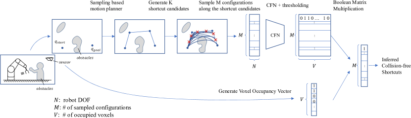
Figure 2: A pipeline of trajectory collision estimation in NN-accelerated trajectory smoother. See Section III for detail.

The pipeline of our NN-based trajectory smoother is illustrated in Fig. 2. Consider a $N$-DOF robot. Given a piecewise linear path (blue lines) in the configuration space, typically outputted by a sampling-based planner, our smoother samples $c$ configurations at regular time-intervals (red X marks), and computes parabolic shortcut trajectories between every pair of sampled configurations. We have $(c+2)$ configurations in total on a given path which consists of the $c$ sampled waypoints plus a starting configuration $q_{start}$ and a goal configuration $q_{goal}$. Let them be $q_{0}...q_{c+1}$, and a shortcut from $q_{i}$ to $q_{j}$ be $S(q_{i},q_{j})$. We have $K=\frac{(c+2)(c+1)}{2}$ shortcut candidates, namely, $S(q_{0},q_{1})$, $S(q_{0},q_{2})$, … $S(q_{0},q_{c+1})$, $S(q_{1},q_{2})$, $S(q_{1},q_{3})$ … $S(q_{1},q_{c+1})$, … $S(q_{c},q_{c+1})$.

Given a shortcut $S(q_{i},q_{j})$, we sample $m_{ij}$ configurations at regular intervals along the shortcut. Next, we stack the $M=\sum_{ij}m_{ij}$ configurations into one single $M\times N$ matrix. This matrix is then fed into the “Clearance Field Neural Network” (CFN, see details in Section III-B) for batch processing. Assume that the spatial workspace is discretized into $V$ voxels, the CFN returns a matrix of size $M\times V$ containing the inferred clearances from the robot placed at every sampled configuration to every voxel of the discretized spatial workspace. Next, we perform thresholding to obtain the $M\times V$ Inferred Collision Matrix: a configuration $q$ is considered as in collision with a voxel if the clearance from the robot placed at $q$ to the voxel is smaller than a given threshold.

In parallel, from the realtime pointcloud captured by the vision system, we generate the $V\times 1$ Voxel Occupancy Vector: an element of this vector is 1 if the corresponding voxel is occupied by an obstacle, 0 if not.

Next, we perform a boolean matrix multiplication of the $M\times V$ Inferred Collision Matrix by the $V\times 1$ Voxel Occupancy Vector to obtain a $M\times 1$ vector that gives the inferred collision status for all the sampled configurations, which in turn yields the inferred collision status for all the $K$ shortcut candidates (a shortcut candidate is in collision if any of its sampled configurations is in collision).

Finally, we run the Dijkstra algorithm to find the shortest trajectory consisting of inferred collision-free shortcuts. We then check the actual collision status of the obtained shortcutted trajectory by a geometric collision checker. If the inference is exact, the shortcutted trajectory should be collision-free and selected. If not, we re-run Dijkstra until an actually collision-free trajectory is found. In practice, owing to the good inference quality, we observed that the shortcutted trajectory returned by the first Dijkstra call is actually collision-free 86.1% of the time.

III-B Clearance Field Network (CFN)

We formally define the clearance of a voxel as the signed-distance between the voxel and the robot surface. Note that the clearance can be negative if the voxel is “inside” the robot. The Clearance Field is then defined as a $V\times 1$ vector that contains all the clearances of the $V$ voxels. Observe that the Clearance Field depends on the robot configuration. A Clearance Field Network is a Neural Network that learns the mapping (see Fig. 3 as well):

$$\mathbb{R}^{N} \rightarrow \mathbb{R}^{V}$$

$$q \mapsto \mathrm{ClearanceField}(q).$$

To learn this mapping, we follow a supervised learning approach: offline, we generate a large number of random configurations. For each configuration $q$, we use a geometric collision-checker (which provides clearance data, such as FCL [23]) to calculate the clearance at every voxel, constructing thereby ClearanceField($q$). At run time, given a new, possibly unseen $q_{\mathrm{new}}$, one can quickly infer ClearanceField($q_{\mathrm{new}}$).

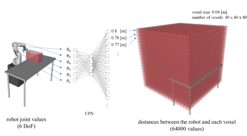
Figure 3: The environment is discretized into $V$ voxels. A voxel’s clearance is the clearance between the voxel and the robot surface. A Clearance Field is a $V\times 1$ vector that contains all the clearances of the $V$ voxels. As the Clearance Field depends on the robot configuration, a Clearance Field Network learns the mapping from a configuration $q$ to its ClearanceField($q$).

The architecture of the proposed Clearance Field Network is shown in Fig. 4. The “sin, cos kernel” converts joint values $q$ to:

$$\textrm{ker}(q)=[\sin(2^{0}\pi q), \cos(2^{0}\pi q),...,$$ (1)

$$\sin(2^{L-1}\pi q),\cos(2^{L-1}\pi q)]$$

inspired by NeRF’s positional encoding [24]. This is intended to increase the frequency of input values and allow the neural network only to learn low-frequency features.

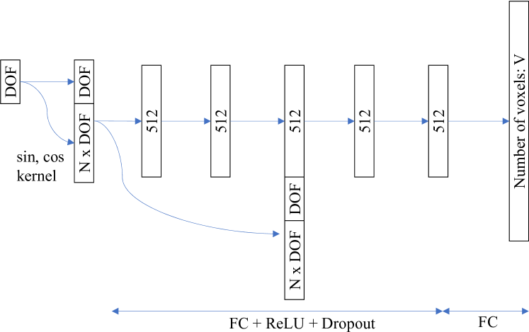
Figure 4: The architecture of Clearance Field Network: Kernel function inputs a high-frequency values into a neural network using sine and cosine. The middle layers are composed of Fully-Connected, ReLU and DropOut with one skip connection.

The advantage of this method is that it can handle dynamic obstacles. Previously, [20] need to feed the information of dynamic obstacles into the neural network. However, since the dimension of input of the neural network should be static and fixed, it is needed to convert the variable size of information about dynamic obstacles into a static-sized feature vector, and feed it into the neural network. In contrast, in our approach, the dynamic obstacles already exist in the form of occupied voxels, whose number is fixed. Our approach can thus apply to any number/shape of dynamic obstacles and the computation can be easily parallelized on GPU.

The reason why we propose to learn clearances instead of directly collision status is that neural networks are better at approximating continuous functions, and clearance is a Lipschitz-continuous function of the environment[20], while collision status is a discrete function.

IV Experiments and Results

IV-A Performance of CFN

First, we examine the clearance field network. We train our neural network with 52,000 joint values and their corresponding clearances using a batch size of 50, validate the training process with 16,000 validation data, and test the trained network with 12,000 test data. During training, we use L1 loss and Adam optimizer [25] with a learning rate of $1\times 10^{-3}$. We set $L=3$ for positional encoding in this experiment. The total data generation takes 2.7 days using 16 CPU cores. The optimization takes 300 iterations (about 1 hour) to converge. Note that the above data generation and optimization steps need to be done only once for a given robot model (without obstacles).The obstacles are handled by the fast inference step at execution time.

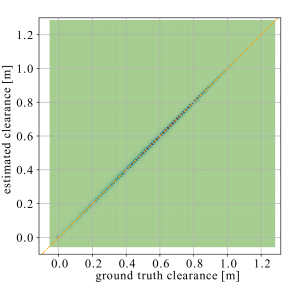
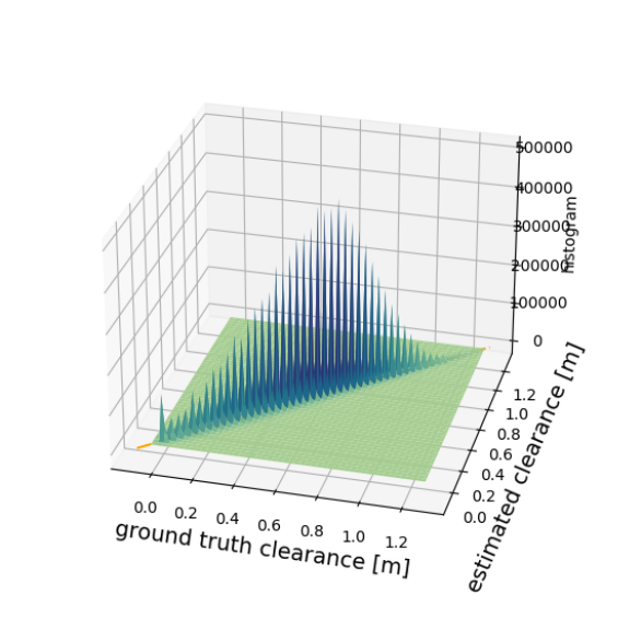
(a) All test results

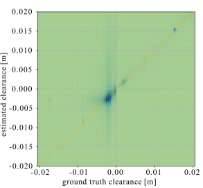
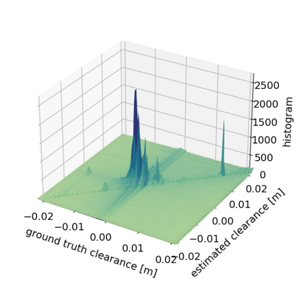
(b) Zoomed in the origin

Figure 5: Colored histograms of Clearance Field Network estimation. Upper: a 2D histogram using all 12,000 test data (left) and its 3D mesh plotting (right). Lower: zoomed in the origin with higher resolution (left) and its 3D mesh plotting (right). An orange dotted line represents a 45 degree line for a reference.

We show colored 2D/3D histograms of clearances estimation in Fig. 5. False negatives (i.e. robot position in collision being classified as free) lead to invalid trajectory and more time for shortcutting, whereas false positives (i.e. collision-free robot position being classified as in collision) lead to conservative shortcutting and a longer trajectory. This trade-off can be managed by a clearance threshold. Precision ($\frac{\mathrm{Estimated\ as\ in\-collision}}{\mathrm{Actually\ in\-collision}}$) is 85.3% and 90.9% when we set a threshold as 20 [mm] and 30 [mm] respectively, which are sufficient to infer the collision status of trajectories. By setting a large threshold, we can reduce the probability to obtain a geometrically in-collision shortcutted trajectory while it may lose a shorter trajectory and vice versa. We use 20 [mm] in our later experiment. Note that safety is always guaranteed because the smoothed trajectory is verified by a geometric collision checker at the end of our pipeline.

IV-B Integration of CFN into a motion planning pipeline

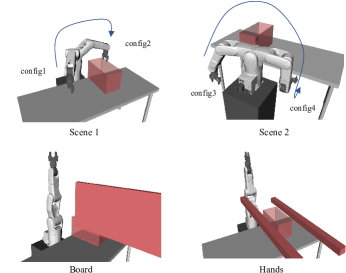
Figure 6: Scenes and Obstacles for trajectory smoothing computation time comparison experiments

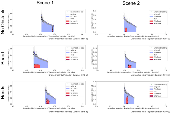
Figure 7: Reduction Ratio of Smoothed Trajectory Duration to Unsmoothed Trajectory Duration to Shortcutting Computation Time [s]. ‘original’ is OpenRAVE’s state-of-the-art parabolic smoother [26, 9]. ‘fcl check’ represents geometric collision checking by FCL[23] and ‘inference’ represents collision inference time. See Section IV-B for detail.

Secondly, we compare our proposed smoother using the trained neural network with OpenRAVE’s state-of-the-art parabolic smoother [26] which originates from [9] and is updated with recent theoretical advancement[27]. In this experiment, given a piecewise linear trajectory from a start to a goal (from ‘config1’ to ‘config2’ in ‘Scene1’, and from ‘config3’ to ‘config4’ in ‘Scene2’ shown in Fig. 6), smoothers smooth the trajectory and we measure their computation time and the duration of its smoothed trajectory under different configurations, changing the maximum number of iterations for the existing method, and the number of sampled waypoints for our proposed method. The clearance threshold for our collision estimation is set to 20 [mm]. We sub-sampled shortcuts at 0.04 seconds interval. Our code is based on OpenRAVE[28] and we use FCL[23] as a collision checking library. All the experiments are done on a single machine, on which Intel^® Xeon^® W-2145 and GeForce GTX 1080 Ti are mounted for CPU and GPU.

In Fig. 7, we plot ratio of smoothed trajectory duration to unsmoothed initial trajectory duration v.s. computation time for each method, where a shorter trajectory and a faster computation time (the left, bottom side of the figure) is preferable. In the existing method, the smoothing time increases as we increase the number of max iterations generating shorter trajectory (blue line), whereas in our method, the smoothing time does not increase constantly as we increase the number of sampled configurations (red line). The result shows that the computation speed of our proposed method is generally 2–3x faster than that of the existing smoother to generate trajectories of the same length, and can generate a much shorter trajectory within the same computation time.

In some cases, e.g. Scene2 with Hands in Fig. 7, the time of geometric collision checking increases to find another collision-free trajectory when false negative collision detection happens, i.e., it can not correctly estimate collision-free trajectories. Statistically, the first inferred collision-free candidate is actually collision-free in 86.1% of 36 cases, and the second, third, and fourth candidates are selected in 2.7% (once), 5.6% (twice) and 2.7% (once) of the cases consecutively.

In terms of optimality, our smoother cannot find an optimal trajectory as we see in Fig. 7. There are several reasons: First, we do not have multi-staged waypoint sampling as it is done in [9], therefore the robot does not accelerate well along the smoothed trajectory. Second, we convert a pointcloud into voxels which include original obstacles. This conversion adds voxel-size padding at maximum to obstacles. Third, we set a clearance threshold in collision estimation, which can also be interpreted as padding and makes the robot larger than its real size, leading to a longer trajectory. However, our focus is not on asymptotical performance but on reducing one-shot smoothing time against computation time, and this non-optimality is acceptable for our use case, i.e., realtime motion planning.

Finally, we conducted a physical robot experiment (Fig. 8). The robot loops between point A and point B while the experimenter randomly introduces obstacles on the robot path. The obstacles are monitored by a Kinect v2 mounted at the side of the workspace, and the obtained pointcloud is converted into a Voxel Occupancy Vector by thresholding the number of points in every voxel at a certain threshold (50 in our experiment) to reduce the effect of sensor noise. By bringing the computation time of the entire Vision–Planning–Execution loop under 300ms, our smoother enables the robot to react to fast perturbations (we observed that using OpenRAVE’s state-of-the-art parabolic smoother, such realtime reaction was not possible as the robot had to stop, take time to compute a new trajectory, and restart), while being smooth (compare with Realtime Robotics’ demo https://vimeo.com/359773568).

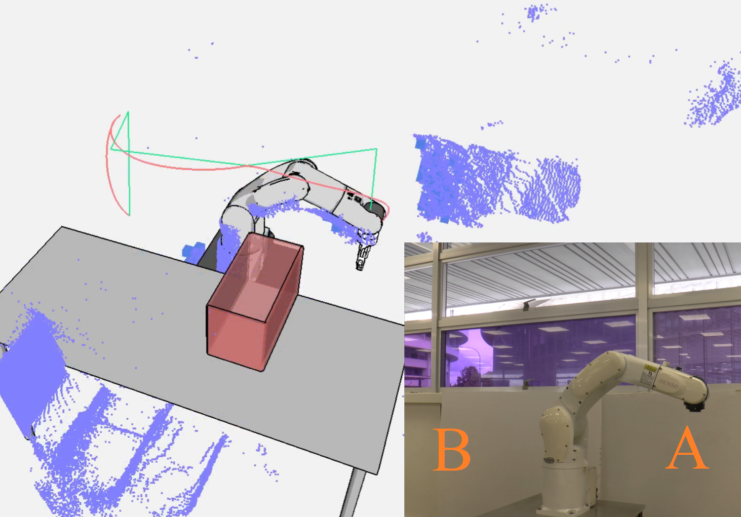
(a)

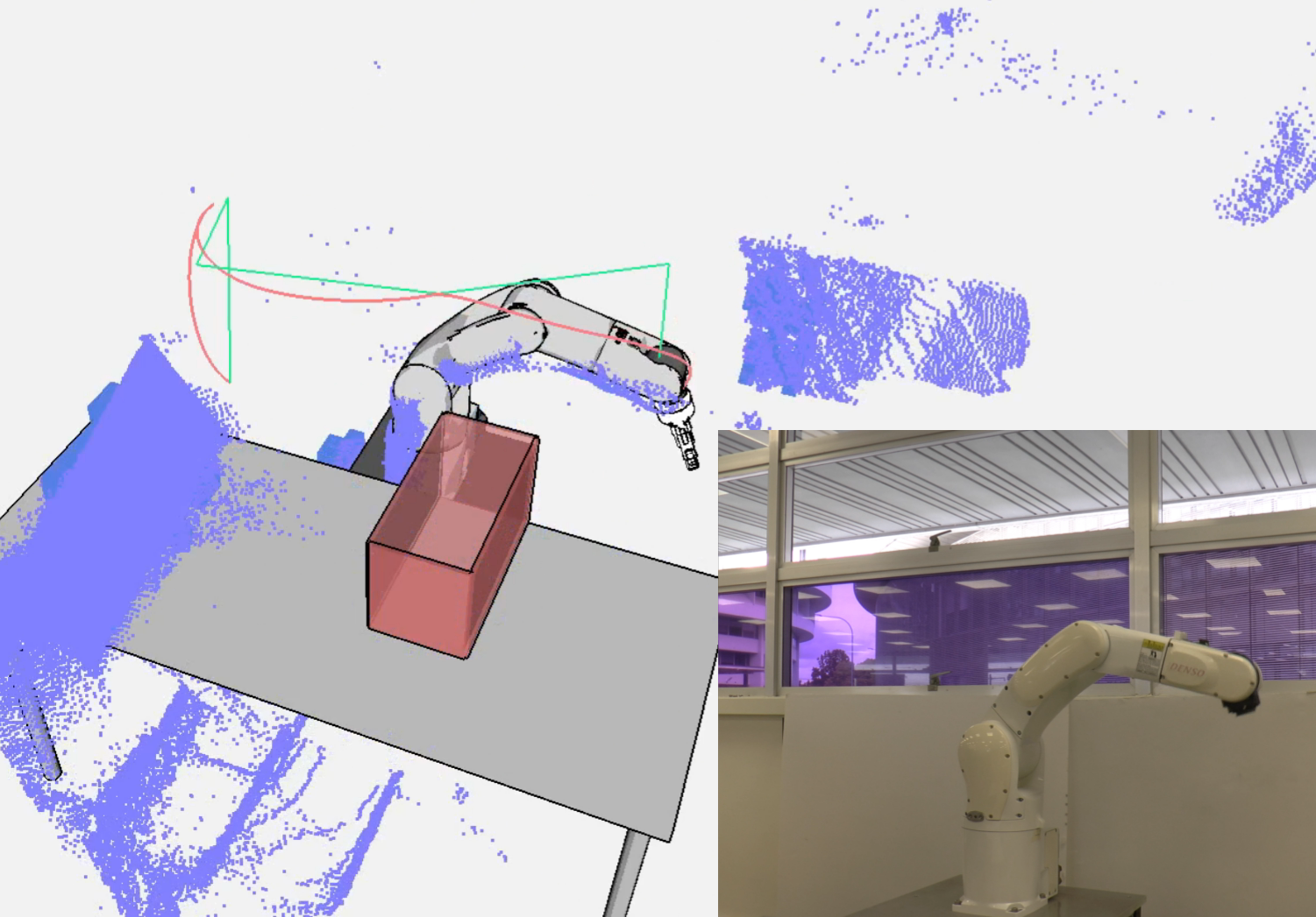
(b)

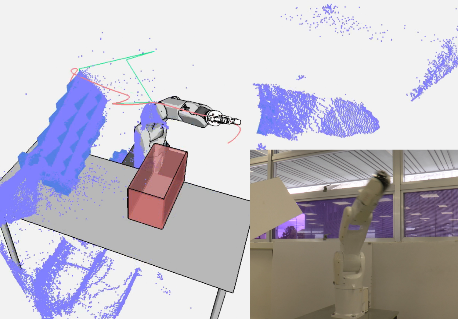
(c)

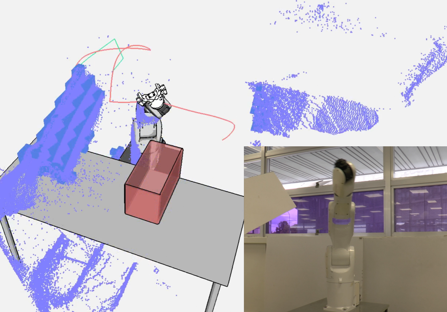
(d)

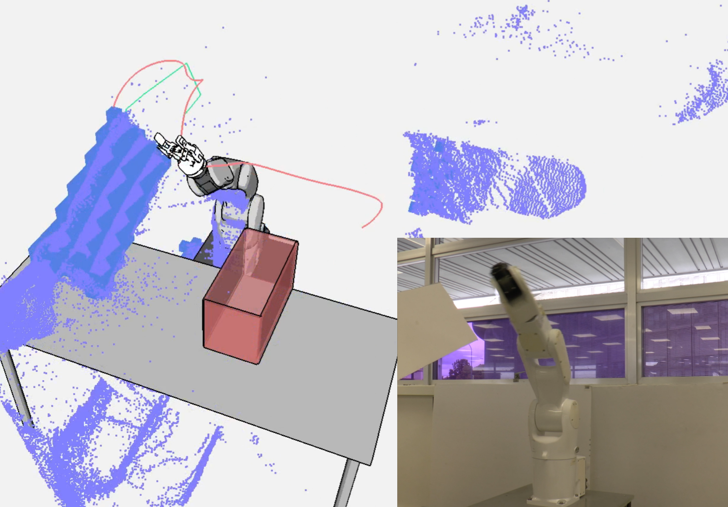
(e)

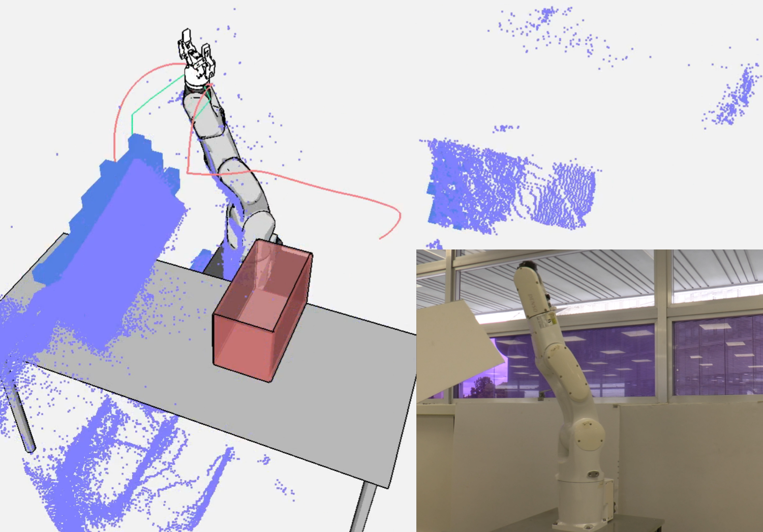
(f)

Figure 8: Realtime Motion Planning and Smoothing on a physical robot. The robot loops between point A and point B while the experimenter randomly introduces an obstacle on the robot path. Purple points: raw point cloud from Kinect v2. Blue boxes: occupied voxels obtained by filtering the raw point cloud. Green line: piecewise linear trajectory output by realtime PRM. Pink line: trajectory smoothed in real time by our smoother. (a) Initial trajectory is planned and the robot starts moving. (b) The experimenter introduces the obstacle after the robot has started moving. (c, d, e, f) As the obstacle approaches and collides with the planned trajectory, replanning with smoothing is triggered and the robot smoothly avoids the obstacle. The full experiment can be viewed at https://youtu.be/XQFEmFyUaj8.

V Conclusion

We have proposed a trajectory smoother by leveraging a neural network to estimate clearances and collisions between a robot and voxels in a parallelized manner. Our planner is 2–3x faster than an existing method, making realtime performance possible.

Why is our smoother faster and can generate shorter trajectory within the same amount of computation time? The reason for shorter trajectory is that our smoother aggressively tries to connect distant waypoints. Even when the number of sampled waypoints is small, our smoother tries to connect waypoints far away from each other (one of them connects a starting point to a goal), so that the computed trajectory tends to be shorter. In contrast, with the existing method, when the number of iterations is small, there is less possibility to connect distant waypoints to have a shorter shortcut. The reason why it is faster is because NN collision estimator can batch-evaluate many waypoints using significantly less time than geometric collision checker.

Currently, there are a number of limitations, which we intend to address in future work.

• Memory consumption and scalability: To find an optimal trajectory as much as possible, we need to increase the number of sampling and have a smaller voxel size, which leads to a larger batch size of input and large memory consumption. Under the configuration in Section IV, our neural network model itself takes about 1.5 GB of GPU memory, and we allocate 0.8 GB of GPU memory for temporary variables. This memory consumption increases in $O(c^{2}VL)$ where $c$ is the number of sampled waypoints, $V$ is the number of voxels and $L$ is the length of the trajectory ($c^{2}$ because we have $K=\frac{(c+2)(c+1)}{2}$ shortcut candidates). Therefore we need to prepare a GPU with large memory to increase the number of sampling waypoints, decrease the resolution of voxels, and apply for a large environment.

• Planning Constraints: Our smoother assumes that collision checking is the bottleneck of trajectory smoothing, i.e., the first shortcut-candidates computation step is much faster than collision checking. If we need to take into account other constraints such as torque limits and robot hand/grasped object’s orientation, the first shortcut computation may become a bottleneck of a whole smoothing pipeline, and this will consequently decrease the speed of our trajectory smoothing. In this case, we need ways to estimate torque and orientation in parallel to utilize our smoothing method.

References

- [1] Steven M. Lavalle. Rapidly-exploring random trees: A new tool for path planning. Technical report, 1998.
- [2] L. E. Kavraki, P. Svestka, J. . Latombe, and M. H. Overmars. Probabilistic roadmaps for path planning in high-dimensional configuration spaces. IEEE Transactions on Robotics and Automation, 12(4):566–580, 1996.
- [3] Jia Pan, Christian Lauterbach, and Dinesh Manocha. g-Planner: Real-time motion planning and global navigation using GPUs. In Twenty-Fourth AAAI Conference on Artificial Intelligence, 2010.
- [4] Jia Pan and Dinesh Manocha. GPU-based parallel collision detection for fast motion planning. The International Journal of Robotics Research, 31(2):187–200, 2012.
- [5] Sean Murray, Will Floyd-Jones, Ying Qi, Daniel Sorin, and George Konidaris. Robot motion planning on a chip. In Proceedings of Robotics: Science and Systems, June 2016.
- [6] Jingru Luo and Kris Hauser. An empirical study of optimal motion planning. In 2014 IEEE/RSJ International Conference on Intelligent Robots and Systems, pages 1761–1768. IEEE, 2014.
- [7] Quang-Cuong Pham and Yoshihiko Nakamura. A new trajectory deformation algorithm based on affine transformations. IEEE Transactions on Robotics, 31(4):1054–1063, 2015.
- [8] Roland Geraerts and Mark H Overmars. Creating high-quality paths for motion planning. The international journal of robotics research, 26(8):845–863, 2007.
- [9] Kris Hauser and Victor Ng-Thow-Hing. Fast Smoothing of Manipulator Trajectories Using Optimal Bounded-Acceleration Shortcuts. In 2010 IEEE International Conference on Robotics and Automation, pages 2493–2498. IEEE, 2010.
- [10] Kourosh Naderi, Joose Rajamäki, and Perttu Hämäläinen. RT-RRT*: A real-time path planning algorithm based on RRT*. In Proceedings of the 8th ACM SIGGRAPH Conference on Motion in Games, MIG ’15, pages 113–118. Association for Computing Machinery, 2015.
- [11] Chonhyon Park, Jia Pan, and Dinesh Manocha. Parallel Motion Planning Using Poisson-Disk Sampling. IEEE Transactions on Robotics, 33(2):359–371, 2017.
- [12] Ran Zhao and Daniel Sidobre. Trajectory smoothing using jerk bounded shortcuts for service manipulator robots. In 2015 IEEE/RSJ International Conference on Intelligent Robots and Systems (IROS), pages 4929–4934, 2015.
- [13] Jia Pan, Liangjun Zhang, and Dinesh Manocha. Collision-free and smooth trajectory computation in cluttered environments. The International Journal of Robotics Research, 31(10):1155–1175, 2012.
- [14] Nathan Ratliff, Matt Zucker, J. Andrew Bagnell, and Siddhartha Srinivasa. CHOMP: Gradient optimization techniques for efficient motion planning. In IEEE International Conference on Robotics and Automation, pages 489–494. IEEE, 2009.
- [15] Mrinal Kalakrishnan, Sachin Chitta, Evangelos Theodorou, Peter Pastor, and Stefan Schaal. STOMP: Stochastic trajectory optimization for motion planning. In 2011 IEEE International Conference on Robotics and Automation, pages 4569–4574, 2011.
- [16] Chonhyon Park, Jia Pan, and Dinesh Manocha. Real-time optimization-based planning in dynamic environments using GPUs. In IEEE International Conference on Robotics and Automation, pages 4090–4097. IEEE, 2013.
- [17] Siyu Dai, Matthew Orton, Shawn Schaffert, Andreas Hofmann, and Brian Williams. Improving Trajectory Optimization Using a Roadmap Framework. In 2018 IEEE/RSJ International Conference on Intelligent Robots and Systems (IROS), pages 8674–8681.
- [18] D. Kappler, F. Meier, J. Issac, J. Mainprice, C. G. Cifuentes, M. Wüthrich, V. Berenz, S. Schaal, N. Ratliff, and J. Bohg. Real-time perception meets reactive motion generation. IEEE Robotics and Automation Letters, 3(3):1864–1871, 2018.
- [19] Daniel Rakita, Bilge Mutlu, and Michael Gleicher. RelaxedIK: Real-time Synthesis of Accurate and Feasible Robot Arm Motion. In Proceedings of Robotics: Science and Systems, Pittsburgh, Pennsylvania, June 2018.
- [20] J. Chase Kew and Brian Ichter and Maryam Bandari and Tsang-Wei Edward Lee and Aleksandra Faust. Neural Collision Clearance Estimator for Batched Motion Planning, 2019.
- [21] Nikhil Das, Naman Gupta, and Michael Yip. Fastron: An online learning-based model and active learning strategy for proxy collision detection. In Conference on Robot Learning, pages 496–504. PMLR, 2017.
- [22] Yuheng Zhi, Nikhil Das, and Michael Yip. DiffCo: Auto-Differentiable Proxy Collision Detection with Multi-class Labels for Safety-Aware Trajectory Optimization, 2021.
- [23] J. Pan, S. Chitta, and D. Manocha. FCL: A general purpose library for collision and proximity queries. In 2012 IEEE International Conference on Robotics and Automation, pages 3859–3866, 2012.
- [24] Ben Mildenhall, Pratul P. Srinivasan, Matthew Tancik, Jonathan T. Barron, Ravi Ramamoorthi, and Ren Ng. NeRF: Representing Scenes as Neural Radiance Fields for View Synthesis, 2020.
- [25] Diederik P. Kingma and Jimmy Ba. Adam: A Method for Stochastic Optimization, 2015.
- [26] Rosen Diankov. ParabolicSmoother - rplanners: OpenRAVE Documentation. http://openrave.org/docs/latest_stable/interface_types/planner/parabolicsmoother/. Last accessed 15 September 2021.
- [27] Puttichai Lertkultanon and Quang-Cuong Pham. Time-optimal parabolic interpolation with velocity, acceleration, and minimum-switch-time constraints. Advanced Robotics, 30(17-18):1095–1110, 2016.
- [28] Rosen Diankov. Automated Construction of Robotic Manipulation Programs. PhD thesis, Carnegie Mellon University, Robotics Institute, August 2010.