Heuristical choice of SVM parameters

Abstract

Support Vector Machine (SVM) is one of the most popular classification methods, and a de-facto reference for many Machine Learning approaches. Its performance is determined by parameter selection, which is usually achieved by a time-consuming grid search cross-validation procedure. There exist, however, several unsupervised heuristics that take advantage of the characteristics of the dataset for selecting parameters instead of using class label information. Unsupervised heuristics, while an order of magnitude faster, are scarcely used under the assumption that their results are significantly worse than those of grid search. To challenge that assumption we have conducted a wide study of various heuristics for SVM parameter selection on over thirty datasets, in both supervised and semi-supervised scenarios. In most cases, the cross-validation grid search did not achieve a significant advantage over the heuristics. In particular, heuristical parameter selection may be preferable for high dimensional and unbalanced datasets or when a small number of examples is available. Our results also show that using a heuristic to determine the starting point of further cross-validation does not yield significantly better results than the default start.

1 Introduction

Support Vector Machine (SVM) is a supervised classification scheme based on ideas developed by V. N. Vapnik and A. Ya. Chervonenkis in 1960s [Schölkopf et al., 2013] and later expanded on in works such as [Cortes and Vapnik, 1995] or [Drucker et al., 1997]. It is based on computing a hyperplane that optimally separates the training examples and then making classification decisions based on the position of a point in relation to that hyperplane. The SVMs have been consistently used in various roles – as an independent classification scheme e.g. [Sha’abani et al., 2020], [Głomb et al., 2018], [Direito et al., 2017], part of more complex engines e.g. [Kim et al., 2003], [Cholewa et al., 2019] or a detection engine e.g. [Ebrahimi et al., 2017], [Chen et al., 2005]. It has been also employed in unsupervised setting in works such as [Lecomte et al., 2011], [Song et al., 2009]. This flexibility allows SVM to be one of the most used machine learning approaches in medicine [Subashini et al., 2009], remote sensing [Romaszewski et al., 2016], threat detection [Parveen et al., 2011], criminology [Wang et al., 2010], photo, text, and time sequence analysis [Li and Guo, 2013].

As a derivation of the hyperplane computation based on a dot product operation, the original SVM derivation – ’linear‘ – has been extended through kernel functions and associated Reproducing Kernel Hilbert Space formalism into ’kernel‘ SVM, which is much more effective in working with different data distributions. A kernel-SVM can use various kernel functions, but the most popular is the Gaussian radial basis function, usually called shortly the Gaussian or RBF kernel. The Gaussian kernel gives one of the best classification performances on a large range of datasets [Fernández-Delgado et al., 2014] and assumes only smoothness of the data, which makes it a natural choice when knowledge about data is limited [Schölkopf and Smola, 1998a]; for those reasons, it is de facto a kernel of choice for application of an SVM classifier.

SVM with a Gaussian kernel has two parameters: the regularization parameter $C$ and the kernel parameter $\gamma$. The former represents a balance between decision function margin and training data classification – large $C$ penalizes misclassification more heavily, producing a better fit to the training data at the cost of making decision surface more complex; smaller $C$ forces larger margin and thus has a regularization effect. The kernel parameter $\gamma$ describes the range of influence of each training example. With $\gamma$ too large, the radius of influence of the support vectors includes only the support vector itself, making the classifier overtrained. With the parameter too small, the decision boundary of each support vector approaches the entire training set. Therefore, the classifier fails to adapt to the often non-linear distribution of classes and kernel SVM is effectively reduced to the linear SVM. Values of these parameters are typically found through supervised search procedures, cross-validation (CV) on the training set and grid-search through a range of predefined parameters [An et al., 2007] [Zhang and Wang, 2016]. A $k$-fold CV separates the data into $k$ folds, with one fold reserved for testing in a round-robin fashion. If parameter optimization is needed, an additional level of CV with $l$ folds is required. With two parameters – e.g. $C$ and $\gamma$ – with $n$ evaluated parameter values each, a total of $kln^{2}$ training runs are required, which can require significant computational resources to perform.

An alternate way of parameter selection is to use the unsupervised heuristical estimation of $C$ and $\gamma$ values. This approach has a number of advantages. If parameter values are estimated in a heuristical fashion, only one level of the CV of $k$ folds is needed for performance evaluation, which is much less computationally expensive. Unsupervised estimation avoids the issues of optimizing parameters on the same set as the one used for training, which can lead to overfitting [Schölkopf and Smola, 1998b]. It is known that in some cases – e.g. with classes conforming to the cluster assumption and Gaussian distribution [Varewyck and Martens, 2010] – optimal or close to optimal parameter values can be analytically derived from data without knowledge about class labels. Unsupervised parameter estimation is an asset in situations, e.g. when additional, non-labelled data are available, or in a semi-supervised classification problem, when only a small fraction of data is labelled [Romaszewski et al., 2016]. The unsupervised estimation has been used as a starting seed for CV grid search, e.g. [Chapelle and Zien, 2005], and some work has been carried on supervised heuristical estimation [Wainer and Fonseca, 2021], but, to our best knowledge, no throughout study for unsupervised parameter estimation has been carried out.

In this work, we experimentally verify the performance of unsupervised heuristical parameter estimation for an SVM classifier (UH-SVM) against a grid search CV trained SVM (GSCV-SVM). Using experiments with a large number of heuristics and a number of popular datasets, we show that while on average GSCV-SVM is more accurate than any tested UH-SVM, without specific prior knowledge of a dataset, there‘s a significantly higher chance of UH-SVM having similar or better accuracy than GSCV-SVM – in terms of statistical significance of the results – than to have a worse accuracy. Considering the aforementioned advantages of the heuristics, in our opinion, this validates the conclusion of UH-SVM parameter estimation being in many application cases on par with the grid search, not only a support method for ’jump starting‘ the GSCV-SVM, as in e.g. [Chapelle and Zien, 2005]. In some cases, in particular, for unbalanced, high-dimensional datasets or when a training set is small, UH-SVM can even outperform GSCV-SVM. Additionally, we show that heuristically estimated parameter values do not give an advantage when used as a seed for standard grid search – e.g. as defined in [Fernández-Delgado et al., 2014]. Our results also show the improvement of both GSCV and UH in relation to default parameter values included in most standard software packages, i.e. $C=1,\gamma=1$. To further explore the topic, we investigate the semi-supervised scenario when the training set is small, also showing the advantage of using UH-SVM approach. Additionally, to present our experimental approach, we perform a unified presentation of heuristical functions reported in the literature, including a generalization of some of them, where their assumptions could be relaxed.

1.1 Related work

One of the early discussions about SVM parameters was provided in [Schölkopf and Smola, 1998b]. In the chapter 7.8, the authors mentioned the grid search CV (GSCV) as a common method of SVM parameter selection. As an alternative, in order to avoid the CV, the authors suggested a number of general approaches including scaling kernel parameters such as the denominator of the RBF kernel so that the kernel values are in the same range. They also suggested that the value of the parameters $C$ can be estimated as $C\propto 1/R^{2}$ where $R$ is some measure of data variability such as standard deviation of the examples from their mean, or the maximum/average distance between examples. Model selection by searching the kernel parameter space was later discussed in [Chapelle and Vapnik, 2000], where authors proposed two simple heuristics based on leave-one-out CV.

Many supervised and often complex heuristics for choosing SVM parameters have been proposed since then, employing e.g. multiverse optimization [Faris et al., 2018], particle swarm [Cho and Hoang, 2017], genetic algorithms [Samadzadegan et al., 2010] and [Phan et al., 2017], gradient descent over the set of parameters [Chapelle et al., 2002], estimation of class separability in the kernel space [Liu et al., 2012]. Alternative approaches have included: iterative, biology-inspired optimisation [Tharwat et al., 2017], applying a one-class SVM to estimate decision boundaries around neighbouring samples [Xiao et al., 2014], simulated annealing [Boardman and Trappenberg, 2006], analysis of support vectors distribution through boundary points[Bi et al., 2005] or simple supervised schemes based on KNN [LáZaro-Gredilla et al., 2012]. A particularly interesting analysis of RBF kernel parameters from the point of view of this paper was proposed in [Varewyck and Martens, 2010]. Authors analysed optimal SVM parameters for Gaussian-distributed data and their work was the basis for e.g. the heuristics proposed in [Wang et al., 2014]. The key point of these works is the optimal value of the parameter $\gamma$ for Gaussian-distributed data.

Unsupervised heuristics are relatively less discussed. A simple heuristic that estimates $\gamma$ as an inverse of some aggregate (e.g. a median) of distances between data points has been proposed in a blog post [Smola, 2011]. In fact, when searching the Internet for a method to choose kernel parameters in an unsupervised way, this post – which refers to the idea from a thesis of B. Schölkopf – is a common find. This heuristics is similar to the ’sigest‘ method [Caputo et al., 2002]. However, even in surveys comparing heuristics for SVM parameter selection [Wainer and Fonseca, 2021] when sigest is considered it is applied to the training set and complimented with cross-validation for the value of the $C$ parameter.

Sometimes, unsupervised heuristics supplement more complex methods, e.g. in [Chapelle and Zien, 2005] authors propose a method for parameter selection inspired by the cluster assumption, based on graph distances between examples in the feature space; a heuristic for unsupervised initialisation of SVM parameters is provided as a starting point of a grid search. Another example are initialisation methods used in well-known ML libraries, e.g. scikit-learn employs its own implementation of heuristic for the $\gamma$ parameter [Gelbart, 2018]; Shark uses the heuristic from [Jaakkola et al., 1999] and while this one is supervised, it can be used in an unsupervised way [Soares et al., 2004].

To conclude, although the idea of unsupervised heuristics for the selection of SVM parameters was already suggested by its authors, such heuristics typically complemented other works and to the best of the authors‘ knowledge, there is no work that collects them together and compares them with each other.

2 Methods

In the following section, we will recall both the ideas behind the Support Vector Machines classifier and the heuristics that we include in our experiments. In some cases our unified presentation of them allows us to derive natural generalizations, e.g. a scaling of [Chapelle and Zien, 2005] in high dimensional datasets or correction for [Soares et al., 2004].

2.1 Support Vector Machines

A kernel SVM [Schölkopf and Smola, 1998b] is a classifier based on the principle of mapping the examples from the input space into a high-dimensional feature space and then constructing a hyperplane in this feature space, with the maximum margin of separation between classes. Let $\mathcal{X}\subset\mathbb{R}^{n}$ be a set of data and let $\mathbf{x}_{i}\in\mathcal{X},i=1,\ldots,m$ be the set of labelled examples. Let also $\mathcal{Y}=\{-1,1\}$ be a set of labels. We define a training set as a set of examples with labels assigned to them,

$$\mathcal{L}=\left\{(\mathbf{x}_{i},y_{i}),i=1,\dots,m\right\}\quad\mathbf{x}_{i}\in\mathcal{X}\quad y_{i}\in\mathcal{Y}.$$ (1)

The SVM assigns an example $\mathbf{x}\in\mathcal{X}\subset\mathbb{R}^{n}$ into one of two classes using a decision function

$$f(\mathbf{x})=\mathrm{sgn}\left(\sum_{i=1}^{m}y_{i}\alpha_{i}K(\mathbf{x},\mathbf{x}_{i})+b\right).$$ (2)

Here, $\alpha_{i}\geq 0$ and $b$ are coefficients computed through Lagrangian optimization – maximization of margin, or distance from hyperplane to classes‘ datapoints on the training set. Training examples $\mathbf{x}_{i}$ where the corresponding values of $\alpha_{i}\neq 0$ are called support vectors (SV). Since SVM is inherently a binary classifier, for multi-class problems several classifiers are combined e.g. using one-against-one method [Hsu and Lin, 2002].

2.1.1 Kernel function

The function $K:\mathcal{X}\times\mathcal{X}\rightarrow\mathbb{R}$ is called the kernel function and it is used to compute the similarity between the classified example $\mathbf{x}$ and each training instance $\mathbf{x}_{i}$. It is a generalization of a dot product operation used in the original linear SVM derivation, i.e. $K(\mathbf{x},\mathbf{x}_{i})=\langle\mathbf{x},\mathbf{x}_{i}\rangle$, taking advantage of the ’kernel trick‘ [Schölkopf and Smola, 1998b] – a non-linear mapping $\phi:\mathcal{X}\rightarrow\mathcal{H}$ to a feature space $\mathcal{H}$ where the dot product is computed by evaluating the value $K(\mathbf{x},\mathbf{x}_{i})=\langle\phi(\mathbf{x}),\phi(\mathbf{x}_{i})\rangle$. The kernel trick allows the SVM to be effectively applied in the case where classes are not linearly separable in the data space. While a number of positive definite symmetric functions can be used as kernels, such as polynomial $K(\mathbf{x},\mathbf{x}_{i})=(\langle\mathbf{x},\mathbf{x}_{i}\rangle+c)^{k}$, $c\geq 0$, $k=1,2,\dots$; Laplace $K(\mathbf{x},\mathbf{x}_{i})=\exp\left(\frac{-||\mathbf{x}-\mathbf{x}_{i}||}{\sigma}\right)$ or Gaussian radial basis function (RBF):

$$K(\mathbf{x},\mathbf{x}_{i})=\text{exp}\left(-\frac{\|\mathbf{x}-\mathbf{x}_{i}\|^{2}}{2\sigma^{2}}\right),$$ (3)

where $\sigma^{2}$ represents the variance of the data and $\|\cdot\|$ is an Euclidean distance in $\mathcal{X}\subset\mathbb{R}^{n}$. This kernel has been found to be the most versatile and effective for many different kinds of data and it will be the focus of our research. By substituting $\gamma=\frac{1}{2\sigma^{2}}$, it can be written:

$$K(\mathbf{x},\mathbf{x}_{i})=\text{exp}\left(-\gamma\|\mathbf{x}-\mathbf{x}_{i}\|^{2}\right),$$ (4)

where $\gamma$ can be viewed as scaling factor, which is one of the parameters of the SVM classifier.

The parameter $\gamma$ controls the impact of individual SV as the kernel distance between two examples decreases with higher values of $\gamma$. Therefore, small values of $\gamma$ will result in many SV influencing the point under test $\mathbf{x}$, producing smooth separating hyperplanes and simpler models. Very small values will lead to all SV having a comparable influence, making the classifier behave like a linear SVM. Large values of $\gamma$ result in more complex separating hyperplanes, better fitting the training data. However, a too high value of $\gamma$ may lead to overtraining (see Figure 1).

2.1.2 Soft margin

In practice, even using a kernel trick, a hyperplane that separates classes may not exist. Therefore, SVM is usually defined as a soft margin classifier by introducing slack variables to relax constraints of Lagrangian optimisation, which allows some examples to be misclassified. It introduces the soft margin parameter $C>0$ where $0<\alpha_{i}<C$ a constraint on $\alpha_{i}$ controlling the penalty on misclassified examples and determining the trade-off between margin maximization and training error minimization. Large values to the parame ter $C$ will result in small number of support vectors while lowering this parameter results in larger number of support vectors and wider margins (see Figure 1).

(a) Good parameter values.

(b) Lower $C$, larger margin.

(c) Lower $C$ and $\gamma$, larger margin, decision boundary ’pushed away‘ from the more compact class.

(d) Very low $\gamma$, decision boundary approaching linear SVM.

(e) High $\gamma$, decision boundary approaching overtraining.

(f) Very high $\gamma$, degenerate decision boundary.

Figure 1: Example SVM behaviour on first two features from the ’Breast Cancer Wisconsin Dataset‘ (wdbc). Red crosses and blue circles mark the position of data points from two classes. Solid line presents the decision boundary, dashed lines denote margin ranges. Presented cases show the example influence of values of $C$ and $\gamma$ parameters, both for good and bad values.

2.2 Unsupervised heuristics for $\gamma$

Unsupervised heuristics usually assume that $\gamma$ should be relative to ’average‘ distance (measured by $\|\cdot\|^{2}$) between the examples from $\mathcal{X}$, so that the two extreme situations – no SV influence or comparable influence of all SV – are avoided. For example, $\gamma$ can be assigned the inverse of the data variance, which corresponds e.g. with heuristics described in [Gelbart, 2018] or [Smola, 2011]). Intuitively then kernel value between two points is a function of how large is the distance between two given points compared to the average distance among the data. Differences between heuristics can be thus reduced to different interpretations of what that average distance is.

2.2.1 $\gamma$ heuristics for Gaussian-distributed data

Considering a pair of examples $(\mathbf{x}_{i},\mathbf{x}_{j})\in\mathcal{X}\times\mathcal{X}\subset\mathbb{R}^{n}\times\mathbb{R}^{n}$ from Gaussian-distributed data, it has been noted in [Varewyck and Martens, 2010], that the squared Euclidean distance $\|\mathbf{x}_{i}-\mathbf{x}_{j}\|^{2}$ is Chi-squared distributed with a mean of $2n\sigma^{2}$, assuming that every data feature has variance $\sigma$ and mean $0$. This observation could be used as a heuristics to estimate the value of $\gamma$ as

$$\gamma=\frac{1}{2n\sigma^{2}}.$$ (5)

If we further assume that $\sigma^{2}=1$ , this simplifies to $\gamma=\frac{1}{2n}$, as noticed by authors of [Wang et al., 2014].

This approach relies on an underlying assumption that data covariance matrix is in the form $\operatorname{Cov}(\boldsymbol{X})=\boldsymbol{I}\sigma^{2}$, which, in turn, means that in a matrix of examples $\boldsymbol{X}\in\mathbb{R}^{m\times n}$, every feature has an equal variance. In practice, data standardisation is used, which divides each feature by its standard deviation. However, the standard deviations are estimated on the training set, and on the test set will produce slightly varying values that are only approximately equal $\sigma_{1}\approx\sigma_{2}\approx\dots\approx\sigma_{n}$. To take that into account, we use another formula for estimation of the value of $\gamma$ as:

$$\gamma=\frac{1}{2\operatorname{Tr}\left(\operatorname{Cov}(\boldsymbol{X})\right)},$$ (6)

where $\operatorname{Tr}(\cdot)$ denotes a trace of a matrix. This heuristic is denoted in the experiments as covtrace.

2.2.2 Smola‘s heuristics

A well-known heuristics for computing the initial value of a parameter $\gamma$ was provided by A. J. Smola in an article on his website [Smola, 2011]. Given examples $(\boldsymbol{x}_{i},\boldsymbol{x}_{j})\in\mathbb{R}^{n}\times\mathbb{R}^{n}$, he considered a kernel function in the form

$$K(\boldsymbol{x}_{i},\boldsymbol{x}_{j})=\kappa(\lambda\|\boldsymbol{x}_{i}-\boldsymbol{x}_{j}\|),$$ (7)

where a scaling factor $\lambda$ of this kernel is to be estimated and $\kappa:\mathbb{R}\rightarrow\mathbb{R}^{+}$. The Smola‘s kernel form is consistent with the RBF kernel given by Eq. (4) – it as special case of (7), with $\kappa(x)=\exp{(-x^{2})}$ where $x\in\mathbb{R}$ and $\lambda=\sqrt{\gamma}$.

He proposes to select a subset of (e.g. $m=1000$) available pairs $(\boldsymbol{x}_{i},\boldsymbol{x}_{j})$ and to compute their distances. Then, the value of $\lambda$ can be estimated as the inverse of $q$ quantile (percentile) of distances where one of three candidates $q\in\{0.1,0.5,0.9\}$ is selected through cross-validation. The reasoning behind those values extends the concept of ’average‘ distance: the value of $q=0.9$ corresponds to the high value of a scaling factor which results in decision boundary that is ’close‘ to SV, $q=0.1$ corresponds to ’far‘ decision boundary, $q=0.5$ aims to balance its distance as ’average‘ decision boundary. The author argues that one of these values in likely to be correct i.e. result in an accurate classifier. Those three $q$ values are included in the experiments as Smola_10, Smola_50 and Smola_90.

2.2.3 Chapelle & Zien $\gamma$ heuristics

A heuristic for choosing SVM parameters can be found in [Chapelle and Zien, 2005]. Interestingly, to the best of our knowledge it is the only method that estimates both $C$ and $\gamma$ in an unsupervised setting (see 2.3.1). The heuristics take into account the density of examples in the data space. Authors introduce a generalization of a ’connectivity‘ kernel, parametrized by $\rho>0$, which in the case of $\rho\rightarrow 0$ defaults to the Gaussian kernel. This kernel proposition is based on minimal $\rho$-path distance $D_{ij}^{\rho}$ which, for $\rho\rightarrow 0$ becomes Euclidean distance i.e. $D_{ij}^{\rho\rightarrow 0}=\|\boldsymbol{x}_{i}-\boldsymbol{x}_{j}\|_{2}$.

Authors use the cluster assumption, by assuming that data points should be considered far from each other when they are positioned in different clusters. In [Chapelle and Zien, 2005] authors consider three classifiers: Graph-based, TSVM and LDS. As this approach introduces additional parameters, which would make cross-validated estimation difficult, authors propose to estimate parameters through heuristics. The value of $\sigma$ (Equation 3) is computed as $\frac{1}{n_{c}}$-th quantile of $\mathcal{D}=\{D_{ij}^{\rho}:\boldsymbol{X}\times\boldsymbol{X}\in\mathbb{R}^{n}\times\mathbb{R}^{n}\}$ where $n_{c}$ is the number of classes. For Gaussian RBF kernel this results in

$$\gamma=\frac{1}{2\text{ quantile}_{\frac{1}{n_{c}}}(\mathcal{D})}$$ (8)

Note that we consider only the case $\rho\rightarrow 0$, as only under this condition heuristics proposed in [Chapelle and Zien, 2005] are comparable with other heuristics presented in this Section and compatible with our experiment. However, the authors‘ original formulation allows for other values of $\rho$. This heuristic, along with the complimentary for the $C$ parameter (see Section 2.3.1) are denoted in the experiments as Chapelle.

2.2.4 Jaakkola‘s and Soares‘ heuristics

The original Jaakkola‘s heuristics was described in [Jaakkola et al., 1999] and [Jaakkola et al., 2000]. It is a supervised heuristics based on median inter-class distance and is computed as follows: for all training examples $\mathbf{x}\in\mathcal{X}\subset\mathbb{R}^{n}$ we define $d_{min}^{l}(\mathbf{x})$ as a distance to its closest neighbour from a different class. Then a set of all nearest neighbour distances is computed as

$$\mathcal{D}^{l}=\left\{d_{min}^{l}(\mathbf{x}):\mathbf{x}\in\mathcal{X}\right\},$$ (9)

and the value of $\sigma=\text{median}(\mathcal{D}^{l})$.

This approach, however, has been interpreted differently in [Soares et al., 2004], which resulted in an unsupervised heuristic based on what was proposed in [Jaakkola et al., 1999]. The approach to estimate $\sigma$ is similar, however, it is calculated without any knowledge about labels of examples, which means that not inter-class but inter-vector distances are used. Considering an unlabelled distance $d_{min}(\mathbf{x})$ of an example $\mathbf{x}$ to its closest neighbour, the set of all neighbour distances is computed as

$$\mathcal{D}=\left\{d_{min}(\mathbf{x}):\mathbf{x}\in\mathcal{X}\right\},$$ (10)

and the value of $\sigma=\text{mean}(\mathcal{D})$. This heuristic is denoted as Soares.

The use of mean instead of median in an approach proposed in [Soares et al., 2004] results in larger values of $\gamma$ in the case of outliers in the data space. Therefore, following the reasoning in the original manuscript [Jaakkola et al., 1999], we propose to compute $\sigma=\text{median}(\mathcal{D})$, which in case of the Gaussian RBF kernel results in:

$$\gamma=\frac{1}{2\text{ median}(\mathcal{D})}.$$ (11)

This heuristic is denoted as Soares_med.

2.2.5 Gelbart‘s heuristics

The heuristic used to estimate the initial value of $\gamma$ in a well-known Python library scikit-learn, was proposed by Michael Gelbart in [Gelbart, 2018]. The scaling factor of Gaussian RBF kernel is computed as

$$\gamma=\frac{1}{n\text{Var}(\mathcal{X})},$$ (12)

where $\mathcal{X}\subset\mathbb{R}^{n}$ and $\text{Var}(\mathcal{X})$ is a variance of all elements in the data set $\mathcal{X}$. It is easy to see that this heuristic is similar to the one discussed in Section 2.2.1, based on [Varewyck and Martens, 2010]: provided that every data feature has variance $\sigma$ and mean $0$ the value of Gelbart‘s heuristics is equal to the one described by Equation 5. The advantage of this heuristics is its computational performance, and it has the potential to perform well when the variance of elements in the data array reflect the variance of the actual data vectors. This heuristic is denoted in our results as Gelbart.

2.3 Unsupervised heuristics for $C$

Unsupervised heuristics for the $C$ parameter are much less common than for $\gamma$; in [Schölkopf and Smola, 1998b], there is a suggestion that parameter $C\propto 1/R^{2}$, where $R$ is a measure for a range of the data in feature space and proposes examples of such $R$ as the standard deviation of the distance between points and their mean or radius of the smallest sphere containing the data. However, to the best of our knowledge, the only actual derivation of this idea was presented in [Chapelle and Zien, 2005], which we discuss below.

2.3.1 Chapelle & Zien $C$ heuristic

Given a $\gamma$ value (originally computed as described in Section 2.2.3), [Chapelle and Zien, 2005] calculate the empirical variance:

$$s^{2}=\frac{1}{m}\sum_{i=1}^{m}K(\mathbf{x}_{i},\mathbf{x}_{i})-\frac{1}{m^{2}}\sum_{i=1}^{m}\sum_{j=1}^{m}K(\mathbf{x}_{i},\mathbf{x}_{j}),$$ (13)

which, with $K(\boldsymbol{x}_{i},\boldsymbol{x}_{i})$ being the value of RBF kernel (4), under the same $\rho\rightarrow 0$ assumption as Section 2.2.3, evaluates to

$$s^{2}=1-a,\qquad a=\frac{1}{m^{2}}\sum_{i=1}^{m}\sum_{j=1}^{m}K(\mathbf{x}_{i},\mathbf{x}_{j}).$$ (14)

The $C$ parameter value is then estimated as

$$C=\frac{1}{s^{2}}.$$ (15)

This heuristic is denoted in our experiments as: Chapelle when used in combination with authors‘ $\gamma$ heuristic (see Section 2.2.3) and +C when used with covtrace heuristic.

2.3.2 A proposed extension of Chapelle & Zien $C$ heuristic

Our observations suggest that values of parameter $C$, when dealing with high-dimensional data such as hyperspectral images, should be higher than estimated with the heuristic proposed in Section 2.3.1. Therefore we propose a new version of the heuristic, by modifying the formula 14. Since in formula 14 the factor $a<1$, higher values of $C$ can be achieved by substituting $s^{2}=1-a^{\prime}$ with $a\leq a^{\prime}<1$.

The value of $a$ in Equation 14 is an average of kernel values for all data points, which, for the RBF kernel, is a function of the average distances between the data points. By selecting a subset of the data points based on values of their distances, we can arbitrarily raise or lower the value of $a$. We start by considering a set of distances between the data points

$$\mathcal{A}=\left\{\|\mathbf{x}_{i}-\mathbf{x}_{j}\|:i,j\leq m;\>\mathbf{x}_{i},\mathbf{x}_{j}\in\mathcal{X}\right\}.$$ (16)

Then we define a subset of distances $\mathcal{A}^{\prime}$ as $\frac{1}{n}$ quantile of $\mathcal{A}$ and we select a relevant set of data points pairs

$$\mathcal{B}=\left\{(i,j):\|\mathbf{x}_{i}-\mathbf{x}_{j}\|\in\mathcal{A}^{\prime}\right\}.$$ (17)

This leads to a modified version of the heuristic

$$s^{2}=1-a^{\prime},\qquad a^{\prime}=\frac{1}{t^{2}}\sum_{(i,j)\in B}K(\mathbf{x}_{i},\mathbf{x}_{j}),$$ (18)

with $t=|\mathcal{B}|$. The rationale of using $\frac{1}{n}$ quantile is that with increased dimension $n$, the proposed condition will restrict the set of pairs $\mathcal{B}$ to the distances between close points. This modified Chapelle‘s heuristic is denoted as +MC, when used with covtrace heuristic for $\gamma$.

2.4 Datasets

Experiments were performed using 31 standard classification datasets obtained from Keel-dataset repository , described in [Alcalá-Fdez et al., 2011]. Instances with missing values and features with zero-variance were removed, therefore the number of examples/features can differ from their version in the UCI [Dua and Graff, 2017] repository. The datasets were chosen to be diverse in regards to the number of features and classes and to include imbalanced cases. In addition, following [Duch et al., 2012], the chosen set includes both complex cases where advanced ML models achieve an advantage over simple methods as well as datasets where most models perform similarly. Reference classification results can be found in[Moreno-Torres et al., 2012] or through OpenML project [Feurer et al., 2021]. The summary of the datasets used in experiments can be found in Table LABEL:tab:datasets.

Before the experiment, every dataset was preprocessed by centering the data and scaling it to the unit variance. This operation was performed using mean and variance values estimated from the training part of the dataset.

[ cap = Datasets, caption = Datasets used in the experiment. Balance is the ratio between size of the smallest and largest class. OA(0R) denotes the accuracy of a zero-rule classifier that predicts the label of the most frequent class., label = tab:datasets, pos = h, doinside = ] lrrrrrl[a]As the dataset is named in KEEL repository https://sci2s.ugr.es/keel/datasets.php Name[a]&ExamplesFeaturesClassesBalanceOA(0R)Notes or full nameappendicitis106720.2580.2balance625430.1746.1Balance Scale DSbanana5300220.8155.2Balance Shape DSbands3651920.5963.0Cylinder Bandscleveland2971350.0853.9Heart Disease (Cleveland), multi-classglass214960.1235.5Glass Identificationhaberman306320.3673.5Haberman‘s Survivalhayes-roth160430.4840.6Hayes-Rothheart2701320.8055.6Statlog (Heart)hepatitis801920.1983.8ionosphere3513320.5664.1iris150431.0033.3Iris plantsled7digit5007100.6511.4LED Display Domainmammographic830520.9451.4Mammographic Massmarketing68761390.4018.3monk-2432620.8952.8MONK‘s Problem 2movement-libras36090151.006.7Libras Movementnewthyroid215530.2069.8Thyroid Disease (New Thyroid)page-blocks54721050.0189.8Page Blocks Classificationphoneme5404520.4270.7pima768820.5465.1Pima Indians Diabetessegment23101971.0014.3sonar2086020.8753.4Sonar, Mines vs. Rocksspectfheart2674420.2679.4SPECTF Hearttae151530.9434.4Teaching Assistant Evaluationvehicle8461840.9125.8Vehicle Silhouettesvowel99013111.009.1Connectionist Benchwdbc5693020.5962.7Breast Cancer Wisconsin (Diagnostic)wine1781330.6839.9wisconsin683920.5465.0Breast Cancer Wisconsin (Original)yeast14848100.0131.2

2.5 Choosing SVM parameters for a given dataset

The experiments used either one or two stages of cross-validation – ’external‘ and ’internal‘ or ’external‘ only – depending on whether the grid search or heuristics were used. Let the heuristics $h\in\mathcal{H}$ from the set of tested heuristics $\mathcal{H}$ be a function that generates SVM parameters $\{C,\gamma\}$ based on a supplied training set $\mathcal{T}$ i.e. $h:\mathcal{T}\rightarrow\mathbb{R}^{2}$. We denote by $h_{0}$ a heuristic which always returns a pair $\{C,\gamma\}=\{1,1\}$, which are commonly assumed defaults, and thus a reference values which are not data-dependent. The $h_{0}$ heuristic is denoted in our experiments as default.

For every training set $\mathcal{T}_{i}$ corresponding with a given $i-$fold of the external CV, and for every heuristics $h\in\mathcal{H}$ parameters of the SVM were selected in three ways:

1. by performing a grid-search around the initial parameters $h_{0}$ and selecting the best model in the internal CV on $\mathcal{T}_{i}$.

2. by applying the heuristics $h(\mathcal{T}_{i})$,

3. by performing a grid-search around the initial parameters $h(\mathcal{T}_{i})$ and selecting the best model in the internal CV on $\mathcal{T}_{i}$.

The range of parameters was $\mathcal{R}=\langle 10^{-5},10^{-4},..,10^{0},..,10^{5}\rangle$, the parameter grid $\mathcal{G}_{h}$ for the heuristics $h$ was generated as

$$\mathcal{G}_{h}=\left\{ri_{\gamma}:r\in\mathcal{R}\right\}\times\left\{ri_{C}:r\in\mathcal{R}\right\},$$ (19)

where $h(\mathcal{T})=(i_{\gamma},i_{C})$. For the external CV, the number of folds $k_{\text{external}}=5$, for the internal CV the number of folds $k_{\text{internal}}=3$; both were stratified CVs.

Two classification performance measures were employed: Overall Accuracy (OA) which is the ratio between a number of correctly classified examples to the total number of examples and Average Accuracy (AA) which is the mean accuracy in classes i.e. the mean between a ratio of correctly classified examples to the total number of examples in every class. The final performance of the classifier in an experiment is the mean OA and AA between external folds. Every experiment was repeated 10 times and the final values of OA and AA were obtained by averaging the performance values of individual runs.

3 Results

Figure 2: Key to the results. This is a cutaway of Figure 3(b), focusing on three selected datasets, which show three general cases of heuristic vs GSCV performance. The values denote difference of a particular heuristic w.r.t. GSCV; bold values denote statistically significant difference. From top: dataset hepatitis – all heuristics, including the default values, fare better than GSCV; dataset glass produces mixed results, some approaches e.g. Gelbart or Chapelle are better, other e.g. covtrace are worse; on the dataset phoneme, all heuristics perform worse than GSCV.

This section looks into differences between OA and AA scores of tested heuristics (including the default, i.e. $C=1,\gamma=1$) vs respective score achieved with the grid search CV (GSCV). When results of individual methods are compared, the statistical significance of the advantage or disadvantage w.r.t the GSCV is confirmed using the one-sided Mann–Whitney–Wilcoxon (MWW) test [Derrick and White, 2017] with the p-value of $p<0.05$. For a given dataset and heuristic, its score can be one of: higher than CV, significant; higher, equal or lower but not significant; lower than CV, significant. Individual results for a given dataset may vary – see Figure 2; we present them as a pair of tables: OA and AA, and as a difference to CV.

Since most of the heuristics only estimate the $\gamma$ parameter, a default value of $C=1$ was used for them.

3.1 Results: Overall Accuracy

The results for OA are presented in Figure 3(a), while the difference in OA between heuristics and CV are in Figure 3(b).

(a) Heuristics OA

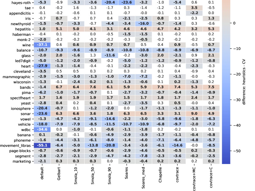
(b) Difference between heuristics and CV

Figure 3: Comparison of overall accuracy (OA) for the experiment comparing parameters obtained with heuristics (H) with the ’default‘ GSCV. In the panel (a) bold font denotes statistical significance of heuristics advantage over GSCV ($p<0.05$). In the right panel, bold font and colour denote statistical significance of difference between H and GSCV. Insignificant differences have white background.

General analysis

Of the 31 datasets tested, GSCV yielded the highest result in 10 cases, 5 of which were statistically significant. This was the best result among all tested methods, as the runner up heuristic covtrace+MC had the highest result in 6 cases. Best results of heuristics against GSCV were from covtrace+C (15 better results, 8 statistically significant), Smola_50 (13 better, 8 statistically significant), Chapelle (13 better, 7 statistically significant) and covtrace+MC (13 better, 6 statistically significant). One can also consider Smola assuming best choice of parameters, simulated by selecting across Smola_10, Smola_50 and Smola_90 (16 better, 8 statistically significant). While GSCV is clearly the best, this advantage is not overwhelming considering it has been outperformed for more than half of the datasets.

In most cases the default parameter values resulted in worse performance than GSCV or the majority of heuristics, which indicates that in order to achieve good classification results parameters must usually be adjusted.

A visualisation of the impact of parameter selection on classification accuracy for six example datasets is presented in Figure 7. Parameter values obtained with unsupervised heuristics along with the default value of SVM parameters are presented in the plots. The five heuristics with the highest results in every image are denoted with coloured marks. In most cases, values obtained using heuristics are located in the areas corresponding to the above-average results of the classifier‘s accuracy, denoted with red colour.

Complexity of data vectors

Using the dimensionality of the data as a measure of data complexity, we have selected eight most complex datasets, with dimension $n\geq 19$: movement-libras, sonar, spectfheart, ionosphere, wdbc, hepatitis, segment, bands. In those datasets GSCV does not fare well – only for segment it has statistically significant highest result of all methods, and even there the difference w.r.t. the runner up (covtrace+MC) is only $0.2$%, arguably a small one. On the other hand four datasets here – sonar, spectfheart, hepatitis, bands – have results where OA for GSCV is statistically significantly worse than all other heuristic (not considering the default). This may result from the fact that in high dimensions the statistics of points distance, which is the base of most heuristical approaches, are more important then class label information. This also suggests that for high dimensional datasets, without a large body of examples, heuristics could be a method of choice for SVM parameter identification. The performance of individual heuristics is comparable, with covtrace+MC having a little advantage.

Large number of vectors

Another analysis concerns datasets with large number of data points available, which, in our experimental setting, translates to large number of training examples. Those datasets, with $m>1000$ examples, are: marketing, page-blocks, phoneme, banana, segment, yeast. Here, the performance of GSCV is generally better in three datasets – highest, statistically significant result for phoneme and segment, and arguably also for banana, in the latter considering lower, but statistically insignificantly, result for Smola_10 and higher for default. That result goes along intuition that many training examples build sufficiently complete image of a whole dataset. GSCV clearly takes advantage of that fact, leading to good parameter choices. Best heuristics here are covtrace, Smola_50 and Gelbart, each with two statistically significant higher results w.r.t. GSCV across datasets in this group.

It is worth noting, however, that for most popular implementations of SVM, the classifier training time increases exponentially with the number of training examples. This means that for this class of datasets, the CV is significantly slower than the heuristic approach.

For dataset with smallest number of examples – six datasets with $m<200$ i.e. hepatitis, appendicitis, iris, tae, hayes-roth, wine – heuristics consistently outperform GSCV, even the default approach; all other have 2 statistically significant results higher than GSCV, with covtrace+C having 3. This contrast with large number of datapoints is expected, but shows clear advantage of heuristics where low number of labelled examples are present.

Highest and lowest overall accuracy

It might be interesting to look at the result from the standpoint of how well SVM is able to ’solve‘ the dataset in general, by which we understand how well SVM classification separates classes with at least one method. On the other side of that spectrum are datasets which are hard for that particular classifier. For that, we select six datasets with best OA (over $97$%): balance, vowel, wine, wdbc, monk-2, wisconsin, along with five datasets with worst OA (under $70$%): glass, yeast, tae, cleveland, marketing.

The first case – the ’best solved‘ datastets – does not show a particular pattern. Two datasets – balance and vowel, first two in terms of OA – have results where GSCV is significantly better, while four remaining ones are inconclusive. Highers results are from Smola_50, Chapelle and covtrace, while highest statistical significant advantage over GSCV belong to Smola_50, Smola_90 and covtrace (two times each).

The situation is different in ’worst solved‘ datasets, where CV never yields the best result, often by a significant margin and is bested by many heuristics. It might suggest that those are the datasets where training examples do not give a good image of the entire dataset and it is preferable to select parameters based on unsupervised information.

High difference between results

It might be interesting to look at datasets where the good or bad parameter selection results in a large change of OA. This would suggest that problem of parameter selection translates very visibly into domain of results. We have selected twelve datasets where the difference between best and worst OA is more than $10$%: movement-libras, wine, wdbc, sonar, heart, hayes-roth, ionosphere, vehicle, newthyroid, vowel, glass, balance. In most cases (7), the spread of results is due to very low score achieved with the default parameter set. Notable higher results are produced with heuristics that estimate $C$ value, i.e. covtrace+C, Chapelle and covtrace+MC, which indicates that when large departure from default parameters is required to achieve a good result, heuristic tuning of both $C$ and $\gamma$ is preferable.

GSCV advantage

Regarding the relation of OA score for GSCV to the next best approach for datasets where GSCV is the highest scoring method: we have selected 7 cases where that difference is higher than $0.1$%: balance, vehicle, phoneme, vowel, led7digit, segment, monk-2. The highest difference is for the balance dataset – $6.9$% – in the remaining cases it is much smaller: $1-2$% for vehicle, phoneme, vowel and under $0.3$% for led7digit, segment, monk-2. While evaluation of a specific percentage value is highly application-dependent, achieving a classification score that differs by no more than 2% from the best result with order of magnitude reduction in execution time – made possible with heuristics through skipping the GSCV – is an attractive option for many real-life applications.

Combining GSCV with heuristics

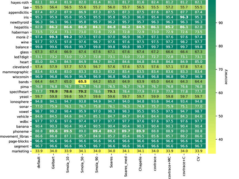
(a) Heuristics OA

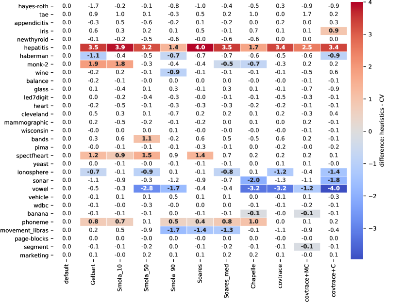
(b) Difference between heuristics+CV and CV

Figure 4: Comparison of overall accuracy (OA) for the experiment comparing parameters obtained with heuristics-centred cross validation (H+CV) with the ’default‘ CV. In the panel (a), bold font denotes statistical significance of (H+CV) advantage over CV ($p<0.05$). In the right panel, bold font and colour denote statistical significance of difference between H+CV and CV. Statistically insignificant differences have white background.

An approach to consider is using the heuristics not in place of GSCV, but as a starting point – to determine the center point of the parameter grid on which, as a second step, GSCV is performed. The results of that experiment can be seen in Figure 4. The main observation is that while adding a heuristical starting point for GSCV produces changes in the results, they are mostly small and statistically insignificant.

It is important that the conclusion that there is no statistical advantage resulting from a better starting point in the GSCV is justified for parameters grids with low density e.g. a common strategy when searched values of $C$ and $\gamma$ differ by an order of magnitude. This issue is discussed in more detail in the Discussion section.

3.2 Results: Average Accuracy

The results for AA are presented in Figure 5(a), while the difference in AA between heuristics and CV are in Figure 5(b).

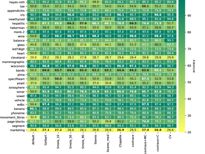
(a) Heuristics AA

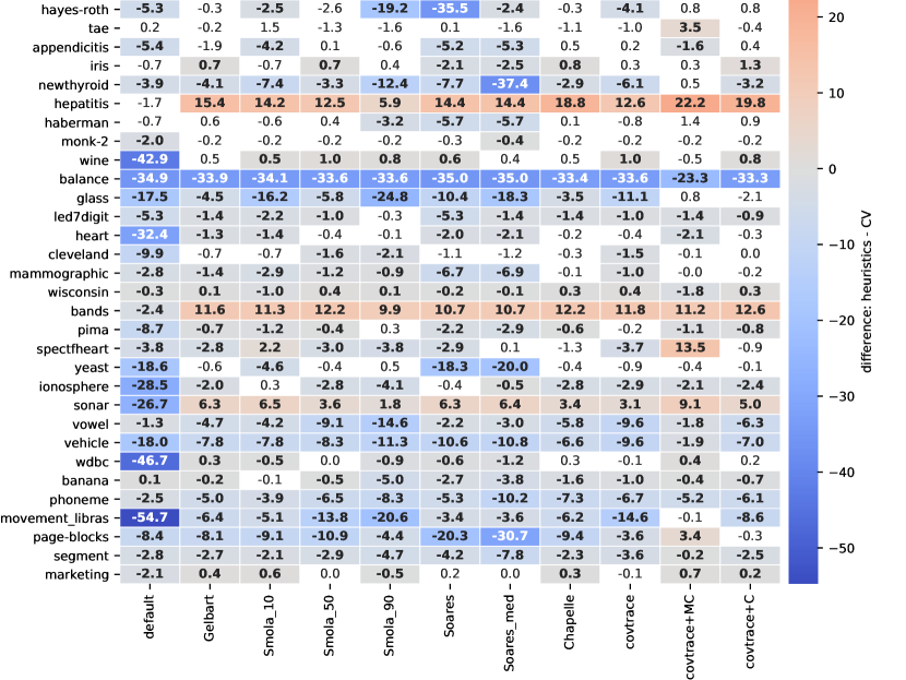
(b) Difference between heuristics and CV

Figure 5: Comparison of average accuracy (AA) for the experiment comparing parameters obtained with heuristics (H) with the ’default‘ CV. In the panel (a) bold font denotes statistical significance of heuristics advantage over CV ($p<0.05$). In the right panel, bold font and colour denote statistical significance of difference between H and CV. Insignificant differences have white background.

General analysis

Considering AA results, the score of GSCV is similar to the OA result; the highest result in 10 cases, 5 of which are statistically significant. A notable result is achieved with the covtrace+MC; 11 times it is better than all other methods, while 13 times it is better than GSCV, with 8 of those statistically significant. Good results are also achieved with covtrace+C, 12 times better than CV, 7 statistically significant and combined Smola, computed as above for OA, 15 times better than CV, 8 statistically significant.

Number of classes

The most numerous in terms of classes are datasets: movement-libras, vowel, yeast, led7digit, marketing, segment, glass, page-blocks, cleveland, all with number of classes $n_{c}\geq 5$. For these datasets GSCV wins 4 times, including 2 times with a statistical advantage. A detailed inspection shows, however, that in this scenario GSCV achieves a statistically significant advantage over most of the heuristics even when it does not yield the best result. On the other spectrum there are fifteen $n_{c}=2$ two-class datasets; heuristics performance is generally comparable for them, 5-7 times higher than GSCV, of those 3-5 are statistically significant. Best performing heuristic is the covtrace+MC. Results indicate that for multi-class datasets GSCV, in terms of AA, performs better then heuristics compared to two-class problems.

Balance of datasets

When considering balance of datasets (see Tab. LABEL:tab:datasets), a set of balanced datasets – with balance value $b>0.9$ – includes iris, segment, movement-libras, vowel, mammographic, tae, vehicle. For them, GSCV has 5 times the highest score, 3 times it is statistically significant; when GSCV does not win, it is usually close behind the leading heuristics. On the contrary, for a set of low balance datasets – with $b<0.2$, yeast, page-blocks, cleveland, glass, balance, hepatitis – GSCV scores highest only once. Results indicate that data set balance works in favor of cross-validation, while imbalance makes heuristics a viable choice.

Combining GSCV with heuristics

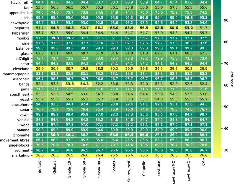
(a) Heuristics AA

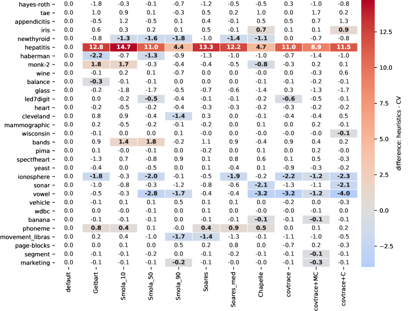
(b) Difference between heuristics+CV and CV

Figure 6: Comparison of average accuracy (AA) for the experiment comparing parameters obtained with heuristics-centred cross validation (H+CV) with the ’default‘ CV. In the panel (a), bold font denotes statistical significance of heuristics advantage over CV ($p<0.05$). In the right panel, bold font and colour denote statistical significance of difference between H and CV. Statistically insignificant differences have white background.

Results are consistent with those for OA: GSCV with unadjusted starting point (anchored at $C=1,\gamma=1$, consistent with the default heuristic) wins only for 5 out of 31 datasets. AA scoring visibly ’flattens‘ the results – there are few cases when heuristics are significantly worse than CV, but also few when they are better.

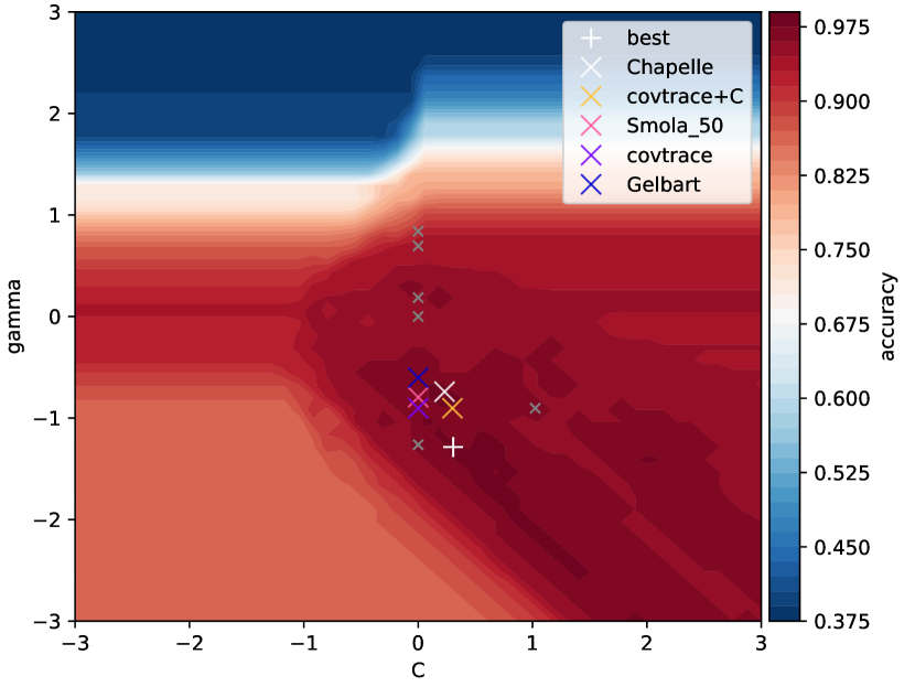
(a) Iris

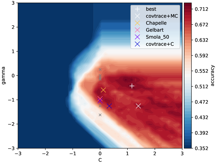
(b) Glass

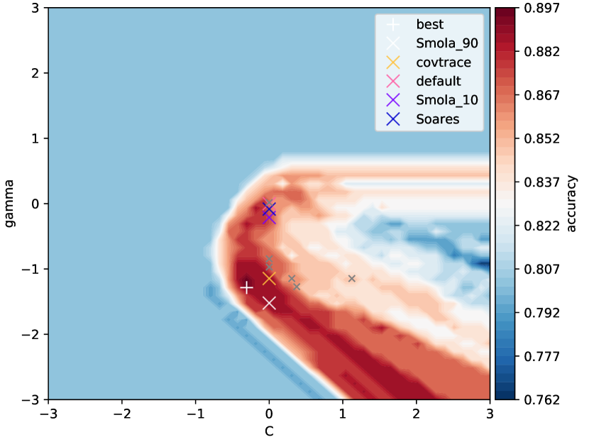
(c) Appendicitis

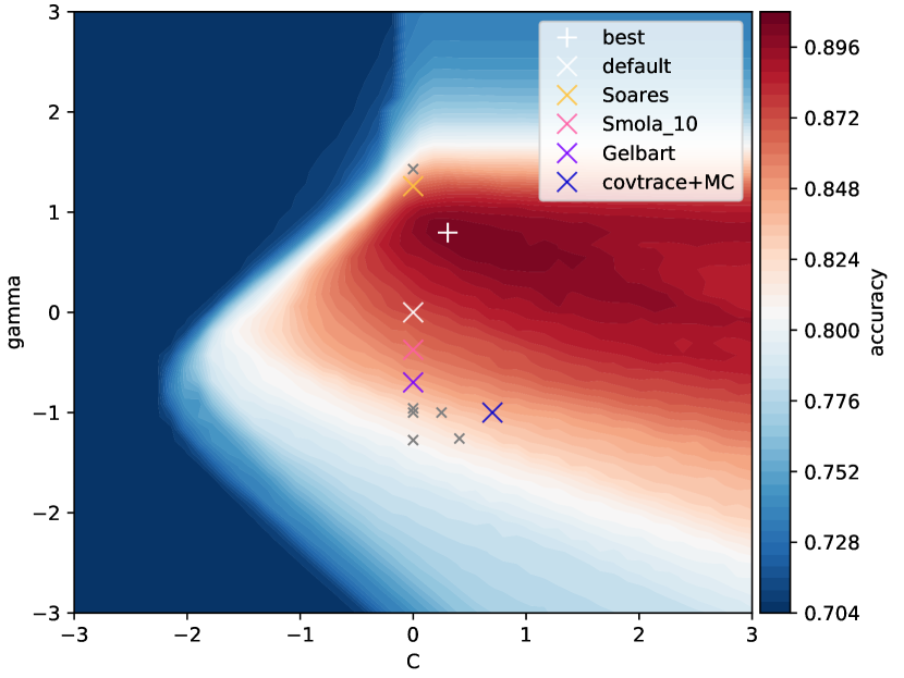
(d) Phoneme

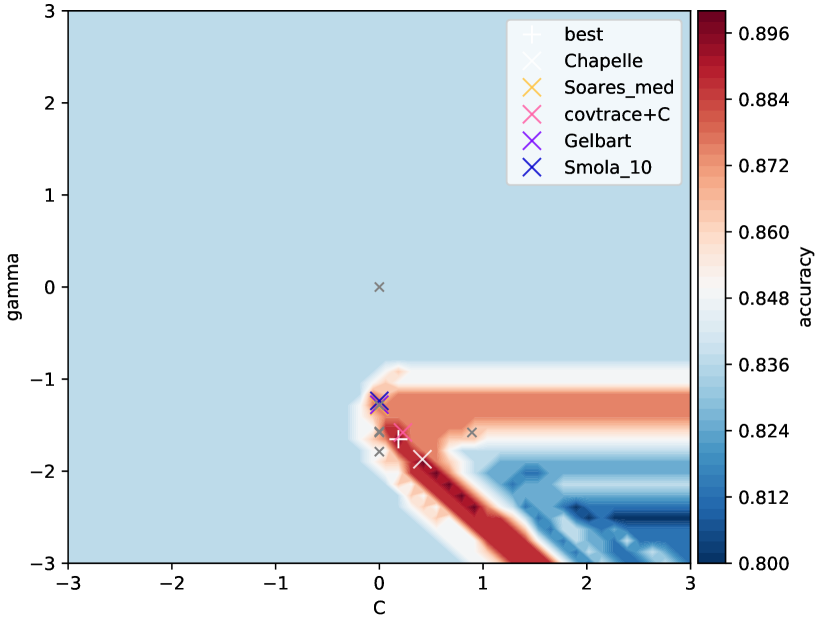
(e) Hepatitis

(f) Bands

Figure 7: The impact of SVM parameters on its accuracy. Parameter values are presented in logspace, and were obtained as a result of a 5-fold CV in grid $50\times 50$ values. The highest value of accuracy is denoted as ’best‘. Marked points denote results of unsupervised heuristics from this paper, with the five heuristics scoring highest marked with colour.

4 Discussion

Results can be discussed in the context of three questions of particular interest to classifier users regarding the validity and strategy of SVM parameter choice as well as initialisation of the parameter search methods.

The first question is: how does the adjustment of classifier parameters affect the expected results in relation to the default values, typically $(1,1)$? Our results indicate that in the majority of cases SVM classifier with parameters adjusted with both GSCV and heuristics outperforms the one with fixed default values. However, this advantage is clearly overwhelming (e.g. the default result is two or three times higher than the second-worst one) for only approximately one-third of the datasets. This may result from the fact that for many testing datasets, good parameter values are located in the area where $\gamma\in\langle 10^{-2},10^{0}\rangle,C\in\langle 10^{0},10^{1}\rangle$ (see Figure 7), which indicates a common structure of data e.g. distances between points or the arrangement of clusters in the dataspace. Since such uniformity may not be the case in a real-life scenario, parameter adjustment is strongly preferred over fixing their values in order to obtain a good representation of SVM performance.

The second issue is whether in the general case the use of unsupervised heuristics for parameter selection results in significantly worse SVM classification performance compared to the supervised GSCV? Based on our results we argue that while GSCV has a statistical advantage over the heuristical approach, this advantage is small and in some cases may even be insignificant. Our arguments are as follows: in our experiments, when GSCV was compared to any of the heuristics, it acquired a significant overall accuracy advantage more often than it was significantly worse. However, at the same time, GSCV produced the best classifier only in about a third of the cases. In the remaining experiments, it was comparable to or worse than heuristics. This observation is supported by inspection of the size of accuracy differences (see Figure 3(b)) which, as explained in Section 3.1, can be viewed as small. It is also supported by inspection of locations for parameters found by heuristics in Figure 7: points that represent heuristics parameters are usually located in areas corresponding to the good performance of the classifier. In some cases such as high-dimensional datasets and ones with a small number of vectors (see Section 3.1), heuristics may lead to a better performing classifier compared to GSCV.

One additional argument to consider is that a scenario used in our experiments when GSCV can use 80% of available data to solve the classification problem can be viewed as optimistic in real-life scenarios. While this proportion is consistent with the general assumption of using ML methods, i.e. that the training set is representative and sufficient for the classification task - in practice the number of learning examples may be smaller, which works in favour of heuristic methods. Considering that the use of heuristics offer an advantage in the computational cost of training a classifier only once, compared to the GSCV where multiple training runs are required, parameter adjustment with unsupervised heuristics seems an alternative worth considering.

The third issue is whether using unsupervised heuristics as a starting point for GSCV may improve SVM classification accuracy compared to a fixed starting point? Results presented in Section 3.1 and Section 3.2 indicate that this is not the case and both scenarios lead to statistically similar classifiers. In our opinion, this results from the strategy of assigning parameters that is common in literature and is described in Section 2.5. The density of the parameter grid where consecutive values of SVM parameters differ by the order of magnitude can be viewed as a compromise between computational complexity and the need to adjust parameter values – in particular to find a correct scale, as indicated in  [Chapelle and Zien, 2005]. The resulting classifier can be expected to be representative of the problem in regards to the accuracy and complexity of its training. Visual inspection of the impact of parameter values on classification accuracy presented in Figure 7 reveals that, usually, at least one of the points corresponding to the values of a parameter grid centred on point $(1,1)$ is located in the area of high results. However, shifting the starting point to one of those returned by heuristics often results in other points shifting outside the high-performing area which results in similar accuracy as in the original grid. On the other hand, using heuristics as a starting point seems to be a good idea when the parameter grid is smaller, which speeds up the classifier training or when the grid has denser sampling which can be viewed as an optimisation of the starting point proposed by heuristics.

Finally, our observations regarding tested unsupervised heuristics for SVM parameter selection can be summarized as follows:

• covtrace - the method and in particular its versions that optimise both parameters i.e. covtrace+C and covtrace+MC performed well both in terms of accuracy and number of advantages over CV. The covtrace+MC seems particularly well suited for high-dimensional data.

• Gelbart - its results were competitive with other methods and, in addition, it is very fast to compute, since it does not require a covariance matrix-like covtrace or distance matrix like the remaining techniques.

• Smola - all three heuristics performed well with Smola_50 obtaining marginally better results. By following the suggestion in  [Smola, 2011], testing a small vector of parameters composed of three values of Smola heuristics may be a compelling alternative to searching the parameter grid.

• Chapelle - the method obtained good results and since it optimises both SVM parameters, this makes it a solid candidate as a method of choice.

• Soares - the method obtained worse results than the reference in our experiments which may suggest an oversimplification of its assumptions in relation to Jaakkola‘s method [Jaakkola et al., 1999] which it is derived from.

4.1 Heuristics in semi-supervised learning

In contrary to the supervised approach where a classifier is trained using a set of labelled examples, a semi-supervised approach uses both labelled and unlabelled data. In many problems such as hyperspectral data classification [Romaszewski et al., 2016], a set of available unlabelled examples is larger than the set of labelled ones, therefore semi-supervised learning allows to obtain higher classification accuracy. However, when the labelled training set is small, parameter selection for the SVM classifier may become hard since the labelled training set alone may not be representative of the features of the whole dataset. Unsupervised heuristics for parameter selection can use both labelled and unlabelled data, which may allow them to obtain parameters better than the CV.

To test this, an experiment described in Section 2.5 was repeated, but the labelled training set used to train the classifier and to perform internal cross-validation was reduced to 10% of its original size (with a minimum of $5$ examples/class). Results of these experiments are presented in Figure 8 in the form of mean accuracy values and differences between mean accuracy obtained with heuristics and CV. When looking at the values of differences in the plot (b), parameters obtained with cross-validation were almost always better than their default values. However, many heuristics and in particular covariance+MC, Gelbert or Chapelle often obtain results comparable or better than cross-validation. The advantage of heuristics is well-visible e.g. for datasets ’cleveland‘, ’sonar‘ and ’bands‘.

The results of the experiment indicate, that unsupervised SVM parameter selection may be a valid approach in a semi-supervised setting with small labelled training sets.

(a) Accuracy for a small training set

(b) Difference between heuristics and CV

Figure 8: Results for a small training set of 10% of the available data. Plot (a) presents OA for SVM parameters obtained with unsupervised heuristics in a semi-supervised scenario i.e. estimating parameters from labelled and unlabelled data. The ’CV‘ column is the result for parameters obtained with an internal 5-fold CV. Plot (b) presents the difference between heuristics and CV results which can be viewed as the advantage of parameter selection with semi-supervised heuristics over the supervised CV approach for a small dataset.

5 Conclusions

The objective of this paper was to investigate the use of heuristics for SVM parameter estimation and compare the performance against grid search cross-validation (GSCV). Our experiments tested ten heuristics or their modifications on thirty-one diverse datasets well-known to the ML community. Such analysis was, to our best knowledge, not performed previously, yet important, as heuristic estimation is an order of magnitude faster than GSCV.

Our results highlight the need for parameter optimisation, as classifiers with parameters tuned with heuristic approach or GSCV significantly outperform ones with fixed, default parameter values. The analysis indicates that while GSCV is on average better than heuristic approach in regards to classification accuracy, this advantage is not large and for many datasets, statistically insignificant. In particular, heuristic parameter selection may be preferable for high dimensional and unbalanced datasets, or when small number of examples is available. On the other hand, GSCV is superior for multiclass, low-dimensional datasets. It seems that combining the heuristic approach and GSCV by choosing a new starting point for the standard parameter grid does not significantly outperform the approach with a default, fixed value $(1,1)$. However, this result likely holds for typically used, relatively sparse and wide parameter grid – for narrow or dense grids adjustment of a starting point with heuristics may be beneficial.

Regarding the choice of heuristics, a good rule of thumb is to choose covtrace+C or Chapelle as they optimise both SVM parameters. Gelbert heuristics seems to be a good choice for setting the $\gamma$ parameter, with an advantage of computational efficiency. A set of three values returned by Smola heuristics may be an effective alternative to predefined values of $\gamma$ in the parameter grid.

We have also noticed the trend in heuristics to undervalue parameter $C$ in cases of the very high dimensionality of the dataset and proposed refinement to Chapelle‘s heuristics to remedy that problem. Our proposed method, denoted covtrace+MC shows good results in the experiments and may be treated as a proof of concept that heuristics might profit from adapting them for high dimensional data.

References

- [Alcalá-Fdez et al., 2011] Alcalá-Fdez, J., Fernández, A., Luengo, J., Derrac, J., García, S., Sánchez, L., and Herrera, F. (2011). Keel data-mining software tool: data set repository, integration of algorithms and experimental analysis framework. Journal of Multiple-Valued Logic & Soft Computing, 17.
- [An et al., 2007] An, S., Liu, W., and Venkatesh, S. (2007). Fast cross-validation algorithms for least squares support vector machine and kernel ridge regression. Pattern Recognition, 40(8):2154–2162.
- [Bi et al., 2005] Bi, L.-P., Huang, H., Zheng, Z.-Y., and Song, H.-T. (2005). New heuristic for determination gaussian kernels parameter. In 2005 International Conference on Machine Learning and Cybernetics, volume 7, pages 4299–4304. IEEE.
- [Boardman and Trappenberg, 2006] Boardman, M. and Trappenberg, T. (2006). A heuristic for free parameter optimization with support vector machines. In The 2006 IEEE International Joint Conference on Neural Network Proceedings, pages 610–617. IEEE.
- [Caputo et al., 2002] Caputo, B., Sim, K., Furesjo, F., and Smola, A. J. (2002). Appearance-based object recognition using SVMs: which kernel should i use? In Proc of NIPS workshop on Statistical methods for computational experiments in visual processing and computer vision, Whistler, volume 2002.
- [Carchedi et al., 2021] Carchedi, N., De Mesmaeker, D., and Vannoorenberghe, L. (2021). Sigest: Hyperparameter estimation for the gaussian radial basis kernel. https://www.rdocumentation.org/packages/kernlab/versions/0.9-29/topics/sigest. RDocumentation, Accessed: 10-06-2021.
- [Chapelle and Vapnik, 2000] Chapelle, O. and Vapnik, V. (2000). Model selection for support vector machines. In Advances in neural information processing systems, pages 230–236.
- [Chapelle et al., 2002] Chapelle, O., Vapnik, V., Bousquet, O., and Mukherjee, S. (2002). Choosing multiple parameters for support vector machines. Machine Learning, 46:131–159.
- [Chapelle and Zien, 2005] Chapelle, O. and Zien, A. (2005). Semi-supervised classification by low density separation. In AISTATS, volume 2005, pages 57–64. Citeseer.
- [Chen et al., 2005] Chen, W.-H., Hsu, S.-H., and Shen, H.-P. (2005). Application of SVM and ANN for intrusion detection. Computers & Operations Research, 32(10):2617–2634.
- [Cho and Hoang, 2017] Cho, M.-Y. and Hoang, T. T. (2017). Feature selection and parameters optimization of SVM using particle swarm optimization for fault classification in power distribution systems. Computational intelligence and neuroscience, 2017.
- [Cholewa et al., 2019] Cholewa, M., Głomb, P., and Romaszewski, M. (2019). A spatial-spectral disagreement-based sample selection with an application to hyperspectral data classification. IEEE Geoscience and Remote Sensing Letters, 16(3):467–471.
- [Cortes and Vapnik, 1995] Cortes, C. and Vapnik, V. (1995). Support-vector networks. Machine learning, 20(3):273–297.
- [Derrick and White, 2017] Derrick, B. and White, P. (2017). Comparing two samples from an individual likert question. International Journal of Mathematics and Statistics, 18(3).
- [Direito et al., 2017] Direito, B., Teixeira, C. A., Sales, F., Castelo-Branco, M., and Dourado, A. (2017). A realistic seizure prediction study based on multiclass SVM. International journal of neural systems, 27(03):1750006.
- [Drucker et al., 1997] Drucker, H., Burges, C. J., Kaufman, L., Smola, A. J., Vapnik, V., et al. (1997). Support vector regression machines. Advances in neural information processing systems, 9:155–161.
- [Dua and Graff, 2017] Dua, D. and Graff, C. (2017). UCI machine learning repository.
- [Duch et al., 2012] Duch, W., Jankowski, N., and Maszczyk, T. (2012). Make it cheap: learning with o(nd) complexity. In The 2012 International Joint Conference on Neural Networks (IJCNN), pages 1–4. IEEE.
- [Ebrahimi et al., 2017] Ebrahimi, M., Khoshtaghaza, M., Minaei, S., and Jamshidi, B. (2017). Vision-based pest detection based on SVM classification method. Computers and Electronics in Agriculture, 137:52–58.
- [Faris et al., 2018] Faris, H., Hassonah, M. A., Ala’M, A.-Z., Mirjalili, S., and Aljarah, I. (2018). A multi-verse optimizer approach for feature selection and optimizing SVM parameters based on a robust system architecture. Neural Computing and Applications, 30(8):2355–2369.
- [Fernández-Delgado et al., 2014] Fernández-Delgado, M., Cernadas, E., Barro, S., and Amorim, D. (2014). Do we need hundreds of classifiers to solve real world classification problems? The journal of machine learning research, 15(1):3133–3181.
- [Feurer et al., 2021] Feurer, M., van Rijn, J. N., Kadra, A., Gijsbers, P., Mallik, N., Ravi, S., Müller, A., Vanschoren, J., and Hutter, F. (2021). OpenML-python: an extensible python API for openml. Journal of Machine Learning Research, 22(100):1–5.
- [Gelbart, 2018] Gelbart, M. (2018). Gamma=‘scale‘ in SVC. https://github.com/scikit-learn/scikit-learn/issues/12741. Accessed: 10-06-2021.
- [Głomb et al., 2018] Głomb, P., Romaszewski, M., Cholewa, M., and Domino, K. (2018). Application of hyperspectral imaging and machine learning methods for the detection of gunshot residue patterns. Forensic Science International, 290:227–237.
- [Hsu and Lin, 2002] Hsu, C.-W. and Lin, C.-J. (2002). A comparison of methods for multiclass support vector machines. IEEE transactions on Neural Networks, 13(2):415–425.
- [Jaakkola et al., 2000] Jaakkola, T., Diekhans, M., and Haussler, D. (2000). A discriminative framework for detecting remote protein homologies. Journal of computational biology, 7(1-2):95–114.
- [Jaakkola et al., 1999] Jaakkola, T. S., Diekhans, M., and Haussler, D. (1999). Using the fisher kernel method to detect remote protein homologies. In ISMB, volume 99, pages 149–158.
- [Kim et al., 2003] Kim, H.-C., Pang, S., Je, H.-M., Kim, D., and Bang, S. Y. (2003). Constructing support vector machine ensemble. Pattern recognition, 36(12):2757–2767.
- [LáZaro-Gredilla et al., 2012] LáZaro-Gredilla, M., GóMez-Verdejo, V., and Parrado-HernáNdez, E. (2012). Low-cost model selection for SVM using local features. Engineering Applications of Artificil Intelligence, 25(6):1203–1211.
- [Lecomte et al., 2011] Lecomte, S., Lengellé, R., Richard, C., Capman, F., and Ravera, B. (2011). Abnormal events detection using unsupervised one-class svm-application to audio surveillance and evaluation. In 2011 8th IEEE International Conference on Advanced Video and Signal Based Surveillance (AVSS), pages 124–129. IEEE.
- [Li and Guo, 2013] Li, X. and Guo, X. (2013). A HOG feature and SVM based method for forward vehicle detection with single camera. In 2013 5th International Conference on Intelligent Human-Machine Systems and Cybernetics, volume 1, pages 263–266. IEEE.
- [Liu et al., 2012] Liu, Z., Zuo, M. J., and Xu, H. (2012). Parameter selection for gaussian radial basis function in support vector machine classification. In 2012 International Conference on Quality, Reliability, Risk, Maintenance, and Safety Engineering, pages 576–581. IEEE.
- [Moreno-Torres et al., 2012] Moreno-Torres, J. G., Sáez, J. A., and Herrera, F. (2012). Study on the impact of partition-induced dataset shift on -fold cross-validation. IEEE Transactions on Neural Networks and Learning Systems, 23(8):1304–1312.
- [Parveen et al., 2011] Parveen, P., Weger, Z. R., Thuraisingham, B., Hamlen, K., and Khan, L. (2011). Supervised learning for insider threat detection using stream mining. In 2011 IEEE 23rd international conference on tools with artificial intelligence, pages 1032–1039. IEEE.
- [Phan et al., 2017] Phan, A. V., Le Nguyen, M., and Bui, L. T. (2017). Feature weighting and SVM parameters optimization based on genetic algorithms for classification problems. Applied Intelligence, 46(2):455–469.
- [Romaszewski et al., 2016] Romaszewski, M., Głomb, P., and Cholewa, M. (2016). Semi-supervised hyperspectral classification from a small number of training samples using a co-training approach. ISPRS Journal of Photogrammetry and Remote Sensing, 121:60–76.
- [Samadzadegan et al., 2010] Samadzadegan, F., Soleymani, A., and Abbaspour, R. A. (2010). Evaluation of genetic algorithms for tuning SVM parameters in multi-class problems. In 2010 11th International Symposium on Computational Intelligence and Informatics (CINTI), pages 323–328.
- [Schölkopf et al., 2013] Schölkopf, B., Luo, Z., and Vovk, V. (2013). Empirical inference: Festschrift in honor of Vladimir N. Vapnik. Springer Science & Business Media.
- [Schölkopf and Smola, 1998a] Schölkopf, B. and Smola, A. J. (1998a). From regularization operators to support vector kernels. Adv. Neural Inf. Process. Syst, 10:343–349.
- [Schölkopf and Smola, 1998b] Schölkopf, B. and Smola, A. J. (1998b). Learning with kernels, volume 4. Citeseer.
- [Sha’abani et al., 2020] Sha’abani, M., Fuad, N., Jamal, N., and Ismail, M. (2020). kNN and SVM classification for EEG: a review. InECCE2019, pages 555–565.
- [Smola, 2011] Smola, A. J. (2011). Easy kernel width choice. https://blog.smola.org/post/940859888/easy-kernel-width-choice. Accessed: 10-06-2021.
- [Soares et al., 2004] Soares, C., Brazdil, P. B., and Kuba, P. (2004). A meta-learning method to select the kernel width in support vector regression. Machine learning, 54(3):195–209.
- [Song et al., 2009] Song, J., Takakura, H., Okabe, Y., and Kwon, Y. (2009). Unsupervised anomaly detection based on clustering and multiple one-class SVM. IEICE transactions on communications, 92(6):1981–1990.
- [Subashini et al., 2009] Subashini, T., Ramalingam, V., and Palanivel, S. (2009). Breast mass classification based on cytological patterns using RBFNN and SVM. Expert Systems with Applications, 36(3):5284–5290.
- [Tharwat et al., 2017] Tharwat, A., Hassanien, A. E., and Elnaghi, B. E. (2017). A BA-based algorithm for parameter optimization of support vector machine. Pattern Recognition Letters, 93:13 – 22. Pattern Recognition Techniques in Data Mining.
- [Varewyck and Martens, 2010] Varewyck, M. and Martens, J.-P. (2010). A practical approach to model selection for support vector machines with a gaussian kernel. IEEE Transactions on Systems, Man, and Cybernetics, Part B (Cybernetics), 41(2):330–340.
- [Wainer and Fonseca, 2021] Wainer, J. and Fonseca, P. (2021). How to tune the RBF SVM hyperparameters? an empirical evaluation of 18 search algorithms. Artificial Intelligence Review, pages 1–27.
- [Wang et al., 2010] Wang, P., Mathieu, R., Ke, J., and Cai, H. (2010). Predicting criminal recidivism with support vector machine. In 2010 International Conference on Management and Service Science, pages 1–9. IEEE.
- [Wang et al., 2014] Wang, X., Huang, F., and Cheng, Y. (2014). Super-parameter selection for gaussian-kernel SVM based on outlier-resisting. Measurement, 58:147–153.
- [Xiao et al., 2014] Xiao, Y., Wang, H., Zhang, L., and Xu, W. (2014). Two methods of selecting gaussian kernel parameters for one-class SVM and their application to fault detection. Knowledge-Based Systems, 59:75 – 84.
- [Zhang and Wang, 2016] Zhang, J. and Wang, S. (2016). A fast leave-one-out cross-validation for SVM-like family. Neural Computing and Applications, 27(6):1717–1730.