From quartic anharmonic oscillator to double well potential

Abstract

It is already known that the quantum quartic single-well anharmonic oscillator $V_{ao}(x)=x^{2}+g^{2}x^{4}$ and double-well anharmonic oscillator $V_{dw}(x)=x^{2}(1-gx)^{2}$ are essentially one-parametric, their eigenstates depend on a combination $(g^{2}\hbar)$. Hence, these problems are reduced to study the potentials $V_{ao}=u^{2}+u^{4}$ and $V_{dw}=u^{2}(1-u)^{2}$, respectively. It is shown that by taking uniformly-accurate approximation for anharmonic oscillator eigenfunction $\Psi_{ao}(u)$, obtained recently, see JPA 54 (2021) 295204 [1] and Arxiv 2102.04623 [2], and then forming the function $\Psi_{dw}(u)=\Psi_{ao}(u)\pm\Psi_{ao}(u-1)$ allows to get the highly accurate approximation for both the eigenfunctions of the double-well potential and its eigenvalues.

I Introduction

For the one-dimensional quantum quartic single-well anharmonic oscillator $V_{ao}(x)=x^{2}+g^{2}x^{4}$ and double-well anharmonic oscillator with potential $V_{dw}(x)=x^{2}(1-gx)^{2}$ the (trans)series in the coupling constant $g$ (which is the Perturbation Theory in powers of $g$ (the Taylor expansion) in the former case of $V_{ao}(x)$ supplemented by exponentially-small terms in $g$ in the latter case of $V_{dw}(x)$) and the semiclassical expansion in $\hbar$ (the Taylor expansion for $V_{ao}(x)$ supplemented by the exponentially small terms in $\hbar$ for $V_{dw}(x)$) for energies coincide Shu-Tur:2018 . This property plays crucially important role in our consideration.

Both the quartic anharmonic oscillator

$$V\ =\ x^{2}+g^{2}x^{4}\ ,$$ (1)

with a single harmonic well at $x=0$ and the double-well potential

$$V\ =\ x^{2}(1-gx)^{2}\ ,$$ (2)

with two symmetric harmonic wells at $x=0$ and $x=1/g$, respectively, are particular cases of the quartic polynomial potential

$$V\ =\ x^{2}+agx^{3}+g^{2}x^{4}\ ,$$ (3)

where $g$ is the coupling constant and $a$ is a parameter. Interestingly, the potential (3) is symmetric for three particular values of the parameter $a$: $a=0$ and $a=\pm 2$. All three potentials (1), (2), (3) belong to the family of potentials of the form

$$V\ =\ \frac{1}{g^{2}}\ {\tilde{V}}(gx)\ ,$$

for which there exists a remarkable property: the Schrödinger equation becomes one-parametric, both the Planck constant $\hbar$ and the coupling constant $g$ appear in the combination $(\hbar g^{2})$, see Shu-Tur:2021 . It can be immediately seen if instead of the coordinate $x$ the so-called classical coordinate $u=(g\,x)$ is introduced. This property implies that the action $S$ in the path integral formalism becomes $g$-independent and the factor $\frac{1}{\hbar}$ in the exponent becomes $\frac{1}{\hbar g^{2}}$ EST:2016 . Formally, the potentials (1)-(2), which enter to the action, appear at $g=1$, hence, in the form

$$V\ =\ u^{2}+u^{4}\ ,$$ (4)

$$V\ =\ u^{2}(1-u)^{2}\ ,$$ (5)

respectively. Both potentials are symmetric with respect to $u=0$ and $u=1/2$, respectively.

Namely, this form of the potentials will be used in this short Note. This Note is the extended version of a part of presentation in AAMP-18 given by the first author AHO-Prague .

II Single-well potential

In AHO for the potential (4) matching the small distances $u\rightarrow 0$ expansion and the large distances $u\rightarrow\infty$ expansion (in the form of semiclassical expansion) for the phase $\phi$ in the representation

$$\Psi\ =\ P(u)\ e^{-\phi(u)}\ ,$$

of the wave function, where $P$ is a polynomial, it was constructed the following function for the $(2n+p)$-excited state with quantum numbers $(n,p)$, $n=0,1,2,\ldots\ ,\ p=0,1$ :

$$\Psi^{(n,p)}_{(approximation)}\ =\$$

$$\frac{u^{p}P_{n,p}(u^{2})}{\left(B^{2}\ +\ u^{2}\right)^{\frac{1}{4}}\left({B}\ +\ \sqrt{B^{2}\ +\ u^{2}}\right)^{2n+p+\frac{1}{2}}}$$

$$\exp\left(-\ \dfrac{A\ +\ (B^{2}+3)\,u^{2}/6\ +\ u^{4}/3}{\sqrt{B^{2}\ +\ u^{2}}}\ +\ \frac{A}{B}\right)\ ,$$ (6)

where $P_{n,p}$ is some polynomial of degree $n$ in $u^{2}$ with positive roots. Here $A=A_{n,p},\ B=B_{n,p}$ are two parameters of interpolation. These parameters $(-A),\ B$ are slow-growing with quantum number $n$ at fixed $p$ taking, in particular, the values

$$A_{0,0}=-0.6244\ ,B_{0,0}=2.3667\ ,$$ (7)

$$A_{0,1}=-1.9289\ ,B_{0,1}=2.5598\ ,$$ (8)

for the ground state and the first excited state, respectively. This remarkably simple function (6), see Fig.1 (top), provides 10-11 exact figures in energies for the first 100 eigenstates. Furthermore, the function (6) deviates uniformly for $u\in(-\infty,+\infty)$ from the exact function in $\sim 10^{-6}$.

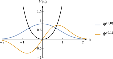
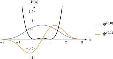
Figure 1: Two lowest, normalized to one eigenfunctions of positive/negative parity: for single-well potential (4), see (6) (top) and for double-well potential (5), see (9)(bottom). Potentials shown by black lines.

III Double-well potential: wavefunctions

Following the prescription, usually assigned in folklore to E.M. Lifschitz - one of the authors of the famous Course on Theoretical Physics by L.D. Landau and E.M. Lifschitz - when a wavefunction for single well potential with minimum at $u=0$ is known, $\Psi(u)$, the wavefunction for double well potential with minima at $u=0,1$ can be written as $\Psi(u)\pm\Psi(u-1)$. This prescription was already checked successfully for the double-well potential (2) in Turbiner:2010 for somehow simplified version of (6), based on matching the small distances $u\rightarrow 0$ expansion and the large distances $u\rightarrow\infty$ expansion for the phase $\phi$ but ignoring subtleties emerging in semiclassical expansion. Taking the wavefunction (6) one can construct

$$\Psi^{(n,p)}_{(approximation)}\ =\$$

$$\frac{P_{n,p}({\tilde{u}}^{2})}{\left(B^{2}\ +\ {\tilde{u}}^{2}\right)^{\frac{1}{4}}\left({\alpha B}\ +\ \sqrt{B^{2}\ +\ {\tilde{u}}^{2}}\right)^{2n+\frac{1}{2}}}$$

$$\exp\left(-\ \dfrac{A\ +\ (B^{2}+3)\,{\tilde{u}}^{2}/6\ +\ {\tilde{u}}^{4}/3}{\sqrt{B^{2}\ +\ {\tilde{u}}^{2}}}\ +\ \frac{A}{B}\right)\ D^{(p)}\ ,$$ (9)

where $p=0,1$ and

$$D^{(0)}\ =\ \cosh\bigg{(}\frac{a_{0}{\tilde{u}}+b_{0}{\tilde{u}}^{3}}{\sqrt{B^{2}+{\tilde{u}}^{2}}}\bigg{)}\ ,$$

$$D^{(1)}\ =\ \sinh\bigg{(}\frac{a_{1}{\tilde{u}}+b_{1}{\tilde{u}}^{3}}{\sqrt{B^{2}+{\tilde{u}}^{2}}}\bigg{)}\ .$$

Here

$$\tilde{u}\ =\ u\ -\ \frac{1}{2}\ ,$$ (10)

$\alpha=1$ and $A,B,a_{0,1},b_{0,1}$ are variational parameters. If $\alpha=0$ as well as $b_{0,1}=0$ the function (9) is reduced to ones which were explored in Turbiner:2010 , see Eqs.(10)-(11). The polynomial $P_{n,p}$ is found unambiguously after imposing the orthogonality conditions of $\Psi^{(n,p)}_{(approximation)}$ to $\Psi^{(k,p)}_{(approximation)}$ at $k=0,1,2,\ldots,(n-1)$, here it is assumed that the polynomials $P_{k,p}$ at $k=0,1,2,\ldots,(n-1)$ are found beforehand.

IV Double-well potential: Results

In this section we present concrete results for energies of the ground state $(0,0)$ and of the first excited state $(0,1)$ obtained with the function (9) at $p=0,1$, respectively. The results are compared with the Lagrange-Mesh Method (LMM) Tur-delValle:2021 .

IV.1 Ground State (0,0)

The ground state energy for (5) obtained variationally using the function (9) at $p=0$ and compared with LMM results Tur-delValle:2021 , where all printed digits (in the second line) are correct,

$$E_{var}^{(0,0)}\ =\ 0.932\,517\,518\,401\ ,$$

$$E_{mesh}^{(0,0)}\ =\ 0.932\,517\,518\,372\ .$$

Note that ten decimal digits in $E_{var}^{(0,0)}$ coincide with ones in $E_{mesh}^{(0,0)}$ (after rounding). Variational parameters in (9) take values,

$$A\ =\ 2.3237\ ,$$

$$B\ =\ 3.2734\ ,$$

$$a_{0}\ =\ 2.3839\ ,$$

$$b_{0}\ =\ 0.0605\ ,$$

cf.(7). Note that $b_{0}$ takes a very small value.

IV.2 First Excited State (0,1)

The first excited state energy for (5) obtained variationally using the function (9) at $p=1$ and compared with LMM results Tur-delValle:2021 , where all printed digits (in the second line) are correct,

$$E_{var}^{(0,1)}\ =\ 3.396\,279\,329\,936\ ,$$

$$E_{mesh}^{(0,1)}\ =\ 3.396\,279\,329\,887\ .$$

Note that ten decimal digits in $E_{var}^{(0,1)}$ coincide with ones in $E_{mesh}^{(0,1)}$ (after rounding). Variational parameters in (9) take values,

$$A\ =\ -2.2957\ ,$$

$$B\ =\ 3.6991\ ,$$

$$a_{1}\ =\ 4.7096\ ,$$

$$b_{1}\ =\ 0.0590\ ,$$

cf.(8). Note that $b_{1}$ takes a very small value similar to $b_{0}$.

V Conclusions

It is presented the approximate expression (9) for the eigenfunctions in the double-well potential (5). In Non-Linearization procedure T:1984 it can be calculated the first correction (the first order deviation) to the function (9). It can be shown that for any $u\in(-\infty,+\infty)$ the functions (9) deviate uniformly from the exact eigenfunctions, beyond the sixth significant figure similarly to the function (6) for the single-well case. It increases the accuracy of the simplified function, proposed in [5] with $\alpha=0$ and $b_{0,1}=0$, in the domain under the barrier $u\in(0.25,0.75)$ from 4 to 6 significant figures leaving the accuracy outside of this domain practically unchanged.