WKB Approximation with Conformable Operator

Abstract

In this paper, the WKB method is extended to be applicable for conformable Hamiltonian systems where the concept of conformable operator with fractional order $\alpha$ is used. The WKB approximation for the $\alpha$-wavefunction is derived when the potential is slowly varying in space. The paper is furnished with some illustrative examples to demonstrate the method. The quantities of the conformable form are found to be in exact agreement with traditional quantities when $\alpha=1$.

Keywords: approximation methods, conformable derivative, conformable Schrodinger equation, conformable Hamiltonian.

1 Introduction

Approximation methods in quantum mechanics, such as the variational method, WKB approximation, and perturbation theory are important tools. Each of these methods has its area of applicability that depend on the nature of the physical system under investigation. The Wentzel-Kramers-Brillouin (WKB) method is useful, with potentials that vary slowly; that is, potentials that remain almost constant over a potential that varies region of the de Broglie Wavelength order. This property, in the case of classical systems, since a classical system’s wavelength reaches zero, the WKB is always fulfilled. It is also possible to consider the approach as a semi-classical approximation[1, 2].

This method is named after Wentzel, Kramers, and Brillouin physicists, all of whom invented it in 1926 [3, 4]. Shortly before that, Harold Jeffreys, a mathematician, had already developed a general method of approximating linear ordinary differential equation solutions in 1923, but the other three were unaware of his work. It is thus commonly referred to today as the WKB or WKBJ approximation [5]. Rabie et.al.[6] were able to quantize constrained systems by using the WKB approximation method, where, after the quantization process, the constraints became conditions to be met in the semiclassical limit on the wave function. Besides, many researchers have used this method to create a quantization process of physical systems[7, 8, 9, 10].

The fractional derivative is as ancient as calculus. In 1695, L’Hospital asked what it meant $\frac{d^{n}f}{dx^{n}}$ if $n=\frac{1}{2}$. Since then, researchers have attempted to describe a fractional derivative. Most of them used an integral form to define the fractional derivative. there many different definitions for fractional derivative,Riemann-Liouville, Caputo, Riesz, Weyl, Grünwald, Riesz-Caputo, Chen, and Hadamard [11, 12, 13, 14, 15, 16, 17, 18, 19, 20, 21]. Two of which are among the most common, Riemann-Liouville and Caputo.

Physicists have investigated WKB approximation process of quantization for the fractional Hamiltonian [22, 23, 24]. A new concept of derivative, called the conformable derivative is given by Khalil et.al.[25], was introduced a few years ago. This description satisfies the conventional derivative’s standard properties. With the emergence of many definitions, the classification of these definitions has started according to the non-locality (Time-based nonlocality is typically called memory) characteristic to local as the conformable derivative, the M-fractional derivative, the alternative fractional derivative, the local fractional derivative, and the Caputo-Fabrizio fractional derivatives with exponential kernels derivative [25, 26, 27, 28, 29, 30, 31], and nonlocal fractional derivative as the Riemann-Liouville, Caputo, Hadamard, Marchaud fractional derivatives[11, 12, 13, 14, 15, 16]. Theoretically, the local derivative is much easier to handle and also obeys certain conventional properties that can not be met by the other derivatives, and it seems to satisfy all the requirements of the standard derivative. For example, the chain law. Thus, the local operator derivative appropriate to extend the WKB approximation.

Recently in ref [32]. Using the conformable operator calculus, the deformation of ordinary quantum mechanics is discussed. The $\alpha$ Hamiltonian operator is suggested and the conformable Schrodinger equation is constructed. Based on that, we quantized fractional harmonic oscillator using creation and annihilation operators in ref [33]. In addition , the conformable calculus was used to extend the perturbation theory to quantum systems containing a conformable derivative of fractional order $\alpha$ in a recent paper [34]. In this work, we would like to extend the WKB approximation to include the conformable derivative of $\alpha$ order.

2 Conformable Derivative

Definition 2.1. Given a function $f\in[0,\infty)\to{R}$. The conformable derivative of $f$ with order $\alpha$ is defined by [25]

$$T_{\alpha}(f)(t)=\lim_{\epsilon\to 0}\frac{f(t+\epsilon t^{1-\alpha})-f(t)}{\epsilon}$$ (1)

for all $t>0$, $\alpha\in(0.1)$ In this paper, we adopt $D^{\alpha}f$ to denote the conformable derivative (CD) of $f$ of order $\alpha$. The properties of this derivative is discussed in detail in Ref [25].
Definition 2.2..$I_{\alpha}^{a}(f)(t)=I_{1}^{a}(t^{\alpha-1}f)=\int_{a}^{t}\frac{f(x)}{x^{1-\alpha}}dx$ where the integral is the usual Riemann improper integral and $\alpha\in(0,1)$. The conformable integral and the conformable derivative obey the following relations

$$D^{\alpha}I_{\alpha}^{a}f(x)=f(x)$$ (2)

$$I_{\alpha}^{a}D^{\alpha}f(x)=f(x)-f(a)$$ (3)

To read more about conformable derivative, its properties, and its applications, we refer you to [35, 36, 37, 38, 39, 40, 41, 42, 43, 44, 45, 46, 47].

3 The conformable quantum mechanics

In terms the conformable derivative, the postulates of conformable quantum mechanics are presented in [48]. The momentum and the coordinate are defined as

$$\hat{x}_{\alpha}=x,~{}~{}~{}\hat{p}_{\alpha}=-i\hbar_{\alpha}^{\alpha}D^{\alpha}_{x},$$ (4)

and $\hbar_{\alpha}^{\alpha}=\frac{h}{(2\pi)^{\frac{1}{\alpha}}}$. In the Hilbert space, the inner product is given by

$$\left<f\vphantom{g}\right|\left.g\vphantom{f}\right>=\int_{-\infty}^{\infty}g^{*}(x)f(x)|x|^{\alpha-1}dx$$ (5)

Thus, the expectation value of an observable $A$ for a system in the state $\psi(x,t)$ is given by

$$\left\langle A\right\rangle =\left<\psi(x,t)\vphantom{A\psi(x,t)}\right|A\left|\psi(x,t)\vphantom{\psi(x,t)A}\right>$$ (6)

$$=\int_{-\infty}^{\infty}\psi^{*}(x,t)A\psi(x,t)|x|^{\alpha-1}dx.$$

In conformable quantum mechanics, the commutator of the $\alpha-$ position operator $\hat{x}_{\alpha}$ and $\alpha-$ momentum operator $\hat{p}_{\alpha}$ is given as [48]:

$$[\hat{x}_{\alpha},\hat{p}_{\alpha}]=i\hbar_{\alpha}^{\alpha}|x|^{1-\alpha}.$$ (7)

Following,Chung et.al [32],the continuity equation is found to be as

$$D^{\alpha}_{t}\rho_{\alpha}(x,t)+D^{\alpha}_{x}j_{\alpha}(x,t)=0$$ (8)

where the $\alpha-$probability density $\rho_{\alpha}(x,t)$ is given as

$$\rho_{\alpha}(x,t)=\psi^{*}\psi,$$ (9)

and the $\alpha-$probability flux $j_{\alpha}(x,t)$ is given as

$$j_{\alpha}(x,t)=\frac{\hbar_{\alpha}^{\alpha}}{2im^{\alpha}}(\psi^{*}D^{\alpha}_{x}\psi-\psi D^{\alpha}_{x}\psi^{*}).$$ (10)

4 Conformable WKB Approximation

To introduce the idea behind this approximation using conformable derivative, we first consider the Schrodinger equation as

$$\frac{\hat{p}_{\alpha}^{2}}{2m^{\alpha}}\psi_{\alpha}(x,t)=(E^{\alpha}-V_{\alpha}(\hat{x}_{\alpha}))\psi_{\alpha}(x,t).$$ (11)

We want to study this conformable Schrodinger equation in two cases.
First case. For constant potential $V_{\alpha}(x)=V^{\alpha}$. Then, we can rewrite eq.(11) as

$$\hat{p}_{\alpha}\psi_{\alpha}(x)=\pm\sqrt{2m^{\alpha}(E^{\alpha}-V^{\alpha})}\psi_{\alpha}(x),$$ (12)

and using eq.(4), we have

$$D^{\alpha}_{x}\psi_{\alpha}(x)=\pm ik\psi_{\alpha}(x),$$ (13)

where $k=\frac{\sqrt{2m^{\alpha}(E^{\alpha}-V^{\alpha})}}{\hbar_{\alpha}^{\alpha}}$. The form of the solution for this conformable differential equation is:

$$\psi_{\alpha}(x)=A\exp{\left(\pm ik\frac{x^{\alpha}}{\alpha}\right)}.$$ (14)

The conformable wave function differs due to two states: classical case and quantum case
1- Classical case: when $E^{\alpha}>V^{\alpha}\to k=\frac{\sqrt{2m^{\alpha}(E^{\alpha}-V^{\alpha})}}{\hbar_{\alpha}^{\alpha}}$, where $k$ is real number thus, the solution for conformable Schrodinger equation in this case is given by eq.(14)
2- Quantum case: when $E^{\alpha}<V^{\alpha}\to k=iq=i\frac{\sqrt{2m^{\alpha}(V^{\alpha}-E^{\alpha})}}{\hbar_{\alpha}^{\alpha}}$, where q is a real number and k is imaginary, thus, the solution for conformable Schrodinger equation, in this case, is given by

$$\psi_{\alpha}(x)=A\exp{\left(\pm q\frac{x^{\alpha}}{\alpha}\right)}.$$ (15)

The conformable wave function $\psi$ is increasing if the sign is positive, and is decreasing if the sign is negative.
Second case. For variable potential $V_{\alpha}(x)$ where the potential is slowly varying. We study this conformable wave function in two cases:
1- Classical case; when $E^{\alpha}>V_{\alpha}(x)$, since there is potential that varies slowly. We expect the solution of conformable Schrodinger equation will be in the form ,

$$\psi_{\alpha}(x)=A(x)\exp{(\pm i\phi(x))},$$ (16)

where $A(x)$ is the amplitude and $\phi(x)$ is the phase, which both depends on $x$.
Thus, we want to calculate $A(x)$ and $\phi(x)$, using

$$D^{\alpha}_{x}D^{\alpha}_{x}\psi(x)=-\frac{\hat{p}_{\alpha}^{2}}{\hbar_{\alpha}^{2\alpha}}\psi(x).$$ (17)

After substituting eq.(16), we have two parts:
- equating real part, we get

$$D^{\alpha}_{x}D^{\alpha}_{x}A(x)-A(x)(D^{\alpha}_{x}\phi(x))^{2}=-\frac{\hat{p}_{\alpha}^{2}}{\hbar_{\alpha}^{2\alpha}}A(x).$$ (18)

- and equating imaginary part, we obtain

$$2D^{\alpha}_{x}A(x)D^{\alpha}_{x}\phi(x)+A(x)D^{\alpha}_{x}D^{\alpha}_{x}\phi(x)=0.$$ (19)

eq.(18) leads to

$$\phi(x)=\pm\frac{1}{\hbar^{\alpha}_{\alpha}}\int p_{\alpha}(x)d^{\alpha}x,$$ (20)

where $D^{\alpha}_{x}D^{\alpha}_{x}A(x)\approx 0$, because $A(x)$ varies slowly, so that the $D^{\alpha}_{x}D^{\alpha}_{x}A(x)$ term is negligible. More precisely, we assume that $\frac{D^{\alpha}_{x}D^{\alpha}_{x}A(x)}{A(x)}$ is much less than both $(D^{\alpha}_{x}\phi(x))^{2}$ and $\frac{\hat{p}_{\alpha}^{2}}{\hbar_{\alpha}^{2\alpha}}$. In that case we can drop the first term of the lift side of eq.(18) But eq.(19) can be rewritten as

$$D^{\alpha}_{x}(A^{2}(x)D^{\alpha}_{x}\phi(x))=0,$$ (21)

where this equation is easily solved

$$A^{2}(x)D^{\alpha}_{x}\phi(x)=c^{2},or\quad A(x)=\frac{c}{\sqrt{D^{\alpha}_{x}\phi(x)}}.$$ (22)

Thus, after substituting $D^{\alpha}_{x}\phi(x)=\frac{\hat{p}_{\alpha}}{\hbar_{\alpha}^{\alpha}}$, we obtain

$$A(x)=\frac{C}{\sqrt{p^{\alpha}(x)}},$$ (23)

where $C=c\sqrt{\hbar_{\alpha}^{\alpha}}$. Then substituting eqs.(20)and(23) in eq.(16), we obtain

$$\psi_{\alpha}(x)=\frac{C}{\sqrt{p^{\alpha}(x)}}\exp{\left(\pm\frac{i}{\hbar^{\alpha}_{\alpha}}\int p^{\alpha}(x)d^{\alpha}x\right)},$$ (24)

which can be written in the following form

$$\psi_{\alpha}(x) =\frac{C_{1}}{\sqrt{p^{\alpha}(x)}}\sin{\left(\frac{1}{\hbar^{\alpha}_{\alpha}}\int p^{\alpha}(x)d^{\alpha}x\right)}$$ (25)

$$+\frac{C_{2}}{\sqrt{p^{\alpha}(x)}}\cos{\left(\frac{1}{\hbar^{\alpha}_{\alpha}}\int p^{\alpha}(x)d^{\alpha}x\right)},$$

2- Quantum case (Tunneling): when $E^{\alpha}<V_{\alpha}(x)$, so, the solution of fractional Schrodinger equation is given by

$$\psi_{\alpha}(x)=\frac{C}{\sqrt{|p^{\alpha}(x)|}}\exp{\left(\pm\frac{1}{\hbar^{\alpha}_{\alpha}}\int|p^{\alpha}(x)|d^{\alpha}x\right)},$$ (26)

where $p^{\alpha}(x)=i\sqrt{2m^{\alpha}(V_{\alpha}(x)-E^{\alpha})}$. We can estimate the probability of transmission in conformable form using [1]

$$T_{\alpha}=\exp{\left(-2\gamma_{\alpha}\right)},$$ (27)

where $\gamma_{\alpha}$ is called the $\alpha-$Gamow factor which is defined as

$$\gamma_{\alpha}=\frac{1}{\hbar^{\alpha}_{\alpha}}\int_{0}^{a}|p^{\alpha}|(x)d^{\alpha}x$$ (28)

5 Alternative approach

We present here an Alternative approach by Making use of the relation between the conformable wave function and the conformable Hamilton’s principal function $S$. The exponential solution of the conformable Schrodinger equation can be written as [1]

$$\psi_{\alpha}(x)=A\exp{\left(\frac{i}{\hbar^{\alpha}_{\alpha}}S(x)\right)}.$$ (29)

The conformable Schrodinger equation for free particle can be written in the form

$$D^{\alpha}_{x}D^{\alpha}_{x}\psi(x)+\frac{p^{2\alpha}}{\hbar_{\alpha}^{2\alpha}}\psi(x)=0.$$ (30)

Substituting eq.(29) in this equation, we have

$$[(D^{\alpha}_{x}S(x))^{2}-i\hbar^{\alpha}_{\alpha}D^{\alpha}_{x}D^{\alpha}_{x}S(x)-p^{2\alpha}]\psi(x)=0.$$ (31)

By writing $S(x)$ as power series of $\hbar^{\alpha}_{\alpha}$

$$S(x)=S_{0}(x)+S_{1}(x)\hbar^{\alpha}_{\alpha}+S_{2}(x)\hbar^{2\alpha}_{\alpha}+\dots,$$ (32)

and substituting in eq.(31), we obtain

$$\hbar^{0}_{\alpha}\to(D^{\alpha}_{x}S_{0}(x))^{2}=p^{2\alpha},$$ (33)

$$\hbar^{\alpha}_{\alpha}\to 2D^{\alpha}_{x}S_{0}(x)D^{\alpha}_{x}S_{1}(x)-iD^{\alpha}_{x}D^{\alpha}_{x}S_{0}(x)=0.$$ (34)

Thus, from these equations we have

$$S_{0}(x)=\pm\int p^{\alpha}d^{\alpha}x,$$ (35)

$$S_{1}(x)=\frac{i}{2}\ln{p^{\alpha}}.$$ (36)

So, after substituting these equations in eq.(29) we obtain

$$\psi_{\alpha}(x)=\frac{A}{\sqrt{p^{\alpha}}}\exp{\left(\pm\frac{i}{\hbar^{\alpha}_{\alpha}}\int p^{\alpha}d^{\alpha}x\right)}.$$ (37)

This result in classical case when $E^{\alpha}>V_{\alpha}(x)$, and for quantum case when $E^{\alpha}<V_{\alpha}(x)$ , so, eq.(37) becomes

$$\psi_{\alpha}(x)=\frac{A}{\sqrt{|p^{\alpha}|}}\exp{\left(\pm\frac{1}{\hbar^{\alpha}_{\alpha}}\int|p^{\alpha}|d^{\alpha}x\right)}.$$ (38)

6 Illustrative Examples

Example 1. A particle free to travel in a small space surrounded by impenetrable barriers defines the infinite potential well. In this model, potential energy is given as

$$V_{\alpha}(x)=\begin{cases}v_{\alpha}(x)&\quad\text{if}\quad 0<x<L\\ \infty&\quad\text{if}\quad x<0,x>L,\end{cases}$$ (39)

where assume the potential $v_{\alpha}(x)$ to be slowly varying . To calculate the fractional energy using eq,(25), with apply the boundary condition of $x=0\to\psi(0)=0,x=L\to\psi(L)=0$, where in $x=0\to\psi(0)=0\to C_{1}\neq 0,C_{2}=0$, thus, using condition $x=L\to\psi(L)=0$, we obtain

$$\phi(L)=\int_{0}^{L}p^{\alpha}(x)d^{\alpha}x=n\pi\hbar^{\alpha}_{\alpha},\quad n=1,2,3,\dots$$ (40)

In special case $V_{\alpha}(x)=0$, we have

$$\phi(L)=\int_{0}^{L}\sqrt{2m^{\alpha}E^{\alpha}}x^{\alpha-1}dx=n\pi\hbar^{\alpha}_{\alpha},$$ (41)

thus, we obtain the conformable energy levels

$$E^{\alpha}=\frac{n^{2}\alpha^{2}\pi^{2}\hbar^{2\alpha}_{\alpha}}{2m^{\alpha}L^{2\alpha}},\quad n=1,2,3,\dots$$ (42)

The conformable wave function is obtained as form

$$\psi_{\alpha}(x)=C_{1}\sqrt{\frac{L^{\alpha}}{n\alpha\pi\hbar^{\alpha}_{\alpha}}}\sin\left(\frac{n\pi x^{\alpha}}{L^{\alpha}}\right),$$ (43)

where $C_{1}=\frac{\alpha\sqrt{2n\pi\hbar^{\alpha}_{\alpha}}}{L^{\alpha}}$ and this equation becomes

$$\psi_{\alpha}(x)=\sqrt{\frac{2\alpha}{L^{\alpha}}}\sin\left(\frac{n\pi x^{\alpha}}{L^{\alpha}}\right).$$ (44)

The Schrodinger for equation infinite potential well is solved by Chung et.al.[32] and they obtained the same result.
Example 2. We consider here the damped harmonic oscillator. The fractional Hamiltonian of damping harmonic oscillator for Bateman system can be written as [49]

$$H_{\alpha}=\frac{(P^{\alpha}_{y})^{2}}{2m^{\alpha}}+\frac{m^{\alpha}}{2}\left(\omega^{2\alpha}-\frac{\lambda^{2}}{4}\right)y^{2\alpha}$$ (45)

$$\quad=-\frac{\hbar^{2\alpha}_{\alpha}}{2m^{\alpha}}D^{\alpha}_{y}D^{\alpha}_{y}+\frac{m^{\alpha}}{2}\left(\omega^{2\alpha}-\frac{\lambda^{2}}{4}\right)y^{2\alpha},$$

$\lambda$ is the damping constant. We assume the damped part is perturbed. To calculate the conformable energy for damping harmonic oscillator (Batman system) using eq.(20), we have

$$\phi=\frac{\sqrt{2m^{\alpha}}}{\hbar^{\alpha}_{\alpha}}\int_{y^{\alpha}_{1}}^{y^{\alpha}_{2}}\sqrt{E^{\alpha}-\frac{m^{\alpha}}{2}\left(\omega^{2\alpha}-\frac{\lambda^{2}}{4}\right)y^{2\alpha}}d^{\alpha}y.$$ (46)

The inflection point when $P^{\alpha}_{y}=0\rightarrow E^{\alpha}=\frac{m^{\alpha}}{2}(\omega^{2\alpha}-\frac{\lambda^{2}}{4})y^{2\alpha}$. So, we get

$$y^{\alpha}_{1}=-\sqrt{\frac{E^{\alpha}}{\frac{m^{\alpha}}{2}\left(\omega^{2\alpha}-\frac{\lambda^{2}}{4}\right)}}\quad,y^{\alpha}_{2}=\sqrt{\frac{E^{\alpha}}{\frac{m^{\alpha}}{2}\left(\omega^{2\alpha}-\frac{\lambda^{2}}{4}\right)}}.$$ (47)

Thus, we find $y^{\alpha}_{1}=-y^{\alpha}_{2}$, and plug in eq.(46), we have

$$\phi=\frac{m^{\alpha}}{\hbar^{\alpha}_{\alpha}}\sqrt{\left(\omega^{2\alpha}-\frac{\lambda^{2}}{4}\right)}\int_{-y^{\alpha}_{2}}^{y^{\alpha}_{2}}\sqrt{\frac{E^{\alpha}}{\frac{m^{\alpha}}{2}\left(\omega^{2\alpha}-\frac{\lambda^{2}}{4}\right)}-y^{2\alpha}}y^{\alpha-1}dy$$ (48)

The solution for this integral is given by

$$\int_{-y^{\alpha}_{2}}^{y^{\alpha}_{2}}\sqrt{\frac{E^{\alpha}}{\frac{m^{\alpha}}{2}\left(\omega^{2\alpha}-\frac{\lambda^{2}}{4}\right)}-y^{2\alpha}}y^{\alpha-1}dy=\frac{y^{2\alpha}_{2}}{\alpha}\frac{\pi}{2}.$$ (49)

So, substituting in eq.(48), we have

$$\phi=\frac{m^{\alpha}}{\hbar^{\alpha}_{\alpha}}\sqrt{\omega^{2\alpha}-\frac{\lambda^{2}}{4}}\frac{y^{2\alpha}_{2}}{\alpha}\frac{\pi}{2},$$ (50)

using connection formula condition [2],

$$\phi=\left(n+\frac{1}{2}\right)\pi.$$ (51)

And, substituting in eq.(50), we have

$$y^{2\alpha}_{2}=\frac{2\alpha\hbar^{\alpha}_{\alpha}}{m^{\alpha}\sqrt{\omega^{2\alpha}-\frac{\lambda^{2}}{4}}}\left(n+\frac{1}{2}\right),$$ (52)

from eq (47) we find $y^{2\alpha}_{2}=\frac{E^{\alpha}}{\frac{m^{\alpha}}{2}(\omega^{2\alpha}-\frac{\lambda^{2}}{4})}$ plug in (52) we get

$$E^{\alpha}=\hbar^{\alpha}_{\alpha}\alpha\sqrt{\omega^{2\alpha}-\frac{\lambda^{2}}{4}}\left(n+\frac{1}{2}\right).$$ (53)

It is in exact agreement with [49], when $\alpha=1$.

Example 3. We consider the potential of alpha particle

$$V_{\alpha}(r)=\begin{cases}\frac{A^{\alpha}}{\alpha r^{\alpha}}&\quad\text{if}\quad r^{\alpha}_{1}<r^{\alpha},\\ 0&\quad\text{if}\quad r^{\alpha}_{1}>r^{\alpha},\end{cases}$$ (54)

where $A^{\alpha}=\frac{2ze^{2}}{4\pi\epsilon_{0}}$.

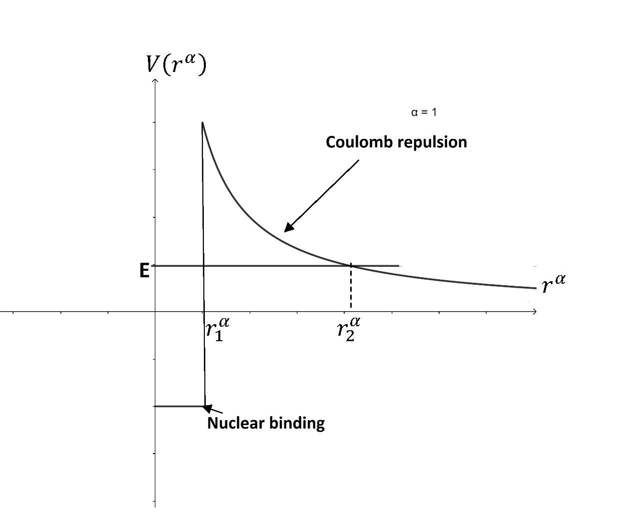
Figure 1: Potential model for $\alpha-$particle’s, in case $\alpha=1$

Here $r_{2}^{\alpha}$ denotes the point where the energy equals the potential which w may call it the conformable turning point. Thus, the conformable energy of alpha particle is given by

$$E^{\alpha}=\frac{A^{\alpha}}{\alpha r_{2}^{\alpha}},$$ (55)

using eq.(28) to calculate transmission probability

$$\gamma_{\alpha}=\frac{1}{\hbar^{\alpha}_{\alpha}}\int_{r_{1}^{\alpha}}^{r_{2}^{\alpha}}\frac{\sqrt{2m^{\alpha}(\frac{A^{\alpha}}{\alpha r^{\alpha}}-E^{\alpha})}}{r^{1-\alpha}}dr$$ (56)

$$\quad=\frac{\sqrt{2m^{\alpha}E^{\alpha}}}{\hbar^{\alpha}_{\alpha}}\int_{r_{1}^{\alpha}}^{r_{2}^{\alpha}}\sqrt{(\frac{r_{2}^{\alpha}}{r^{\alpha}}-1)}r^{\alpha-1}dr$$

$$\quad=\frac{\sqrt{2m^{\alpha}E^{\alpha}}}{\hbar^{\alpha}_{\alpha}}[r_{2}^{\alpha}\arccos{\sqrt{\frac{r_{1}^{\alpha}}{r_{2}^{\alpha}}}}-\sqrt{r_{1}^{\alpha}(r_{2}^{\alpha}-r_{1}^{\alpha})}].$$

In case $r_{1}^{\alpha}\ll r_{2}^{\alpha}\to\arccos{\sqrt{\frac{r_{1}^{\alpha}}{r_{2}^{\alpha}}}}\approx\frac{\pi}{2}-\sqrt{\frac{r_{1}^{\alpha}}{r_{2}^{\alpha}}}$ and $r_{2}^{\alpha}-r_{1}^{\alpha}\approx r_{2}^{\alpha}$, so we have

$$\gamma_{\alpha}=\frac{\sqrt{2m^{\alpha}E^{\alpha}}}{\hbar^{\alpha}_{\alpha}}[r_{2}^{\alpha}\frac{\pi}{2}-2\sqrt{r_{1}^{\alpha}r_{2}^{\alpha}}].$$ (57)

Substituting value of $r_{2}^{\alpha}$ from eq.(55), we have

$$\gamma_{\alpha}=K_{1}^{\alpha}(\pi\sqrt{2})^{1-\alpha}\frac{z^{\alpha}}{\alpha\sqrt{E^{\alpha}}}-K_{2}^{\alpha}4^{1-\alpha}\sqrt{\frac{r_{1}^{\alpha}z^{\alpha}}{\alpha}},$$ (58)

where $K_{1}=\frac{e^{2}\pi\sqrt{2m}}{4\pi\epsilon_{0}\hbar}=1.986MeV$ and $K_{2}=(\frac{e^{2}m}{4\pi\epsilon_{0}})^{\frac{1}{2}}\frac{4}{\hbar}=1.485MeV$ [1]. Thus, after substituting this equation in eq.(27), we have

$$T=\exp{-2\left(K_{1}^{\alpha}(\pi\sqrt{2})^{1-\alpha}\frac{z^{\alpha}}{\alpha\sqrt{E^{\alpha}}}-K_{2}^{\alpha}4^{1-\alpha}\sqrt{\frac{r_{1}^{\alpha}z^{\alpha}}{\alpha}}\right)}.$$ (59)

It is in exact agreement with [1], when $\alpha=1$.

7 Summary and conclusion

The WKB approximation is extended to be applicable for $\alpha-$Hamiltonian in the conformable form. The conformable derivative of $\alpha$ fractional order is used and applied to three illustrative examples. Quantities were obtained in the conformable form so that the corresponding the traditional forms are recovered when $\alpha=1$

References

- [1] D. J. Griffiths and D. F. Schroeter, Introduction to quantum mechanics. Cambridge University Press, 2018.
- [2] N. Zettili, “Quantum mechanics: concepts and applications,” 2003.
- [3] H. A. Kramers, “Wellenmechanik und halbzahlige quantisierung,” Zeitschrift für Physik, vol. 39, no. 10-11, pp. 828–840, 1926.
- [4] G. Wentzel, “Eine verallgemeinerung der quantenbedingungen für die zwecke der wellenmechanik,” Zeitschrift für Physik, vol. 38, no. 6-7, pp. 518–529, 1926.
- [5] H. Jeffreys, “On certain approximate solutions of lineae differential equations of the second order,” Proceedings of the London Mathematical Society, vol. 2, no. 1, pp. 428–436, 1925.
- [6] E. M. Rabei, K. I. Nawafleh, and H. B. Ghassib, “Quantization of constrained systems using the wkb approximation,” Physical Review A, vol. 66, no. 2, p. 024101, 2002.
- [7] E. M. Rabei, “Quantization of christ—lee model using the wkb approximation,” International Journal of Theoretical Physics, vol. 42, no. 9, pp. 2097–2102, 2003.
- [8] K. I. Nawafleh, E. M. Rabei, and H. B. Ghassib, “Quantization of reparametrized systems using the wkb method,” Turkish Journal of Physics, vol. 29, no. 3, pp. 151–162, 2005.
- [9] E. M. Rabei, E. H. Hassan, H. B. Ghassib, and S. Muslih, “Quantization of second-order constrained lagrangian systems using the wkb approximation,” International Journal of geometric methods in modern Physics, vol. 2, no. 03, pp. 485–504, 2005.
- [10] E. H. Hasan, E. M. Rabei, and H. B. Ghassib, “Quantization of higher-order constrained lagrangian systems using the wkb approximation,” International Journal of Theoretical Physics, vol. 43, no. 11, pp. 2285–2298, 2004.
- [11] M. Caputo, “Linear models of dissipation whose Q is almost frequency independent—II,” Geophysical Journal International, vol. 13, no. 5, pp. 529–539, 1967, publisher: Blackwell Publishing Ltd Oxford, UK.
- [12] K. Oldham and J. Spanier, The fractional calculus theory and applications of differentiation and integration to arbitrary order. Elsevier, 1974.
- [13] K. S. Miller and B. Ross, An introduction to the fractional integrals and derivatives-theory and applications. Wiley, New York, 1993.
- [14] A. Kilbas, Theory and applications of fractional differential equations.
- [15] R. Hilfer, Applications of fractional calculus in physics. World scientific Singapore, 2000, vol. 35, no. 12.
- [16] I. Podlubny, Fractional differential equations: an introduction to fractional derivatives, fractional differential equations, to methods of their solution and some of their applications. Elsevier, 1998.
- [17] M. Klimek, “Lagrangean and Hamiltonian fractional sequential mechanics,” Czechoslovak Journal of Physics, vol. 52, no. 11, pp. 1247–1253, 2002, publisher: Springer.
- [18] W. Chen, X.-D. Zhang, and D. Korošak, “Investigation on fractional and fractal derivative relaxation-oscillation models,” International Journal of Nonlinear Sciences and Numerical Simulation, vol. 11, no. 1, pp. 3–10, 2010, publisher: De Gruyter.
- [19] J.-H. He, “A new fractal derivation,” Thermal Science, vol. 15, no. suppl. 1, pp. 145–147, 2011.
- [20] R. Gorenflo and F. Mainardi, “Essentials of fractional calculus,” 2000, publisher: Citeseer.
- [21] J. M. Kimeu, “Fractional calculus: Definitions and applications,” 2009.
- [22] E. M. Rabei, I. M. Altarazi, S. I. Muslih, and D. Baleanu, “Fractional wkb approximation,” Nonlinear Dynamics, vol. 57, no. 1-2, pp. 171–175, 2009.
- [23] K. Sayevand and K. Pichaghchi, “A modification of $$$\backslash$mathsf ${$$}$ $$ method for fractional differential operators of Schrödinger’s type,” Analysis and Mathematical Physics, vol. 7, no. 3, pp. 291–318, 2017, publisher: Springer.
- [24] E. M. Rabei and M. Al Horani, “Quantization of fractional singular lagrangian systems using wkb approximation,” International Journal of Modern Physics A, vol. 33, no. 36, p. 1850222, 2018.
- [25] R. Khalil, M. Al Horani, A. Yousef, and M. Sababheh, “A new definition of fractional derivative,” Journal of Computational and Applied Mathematics, vol. 264, pp. 65–70, 2014.
- [26] U. N. Katugampola, “A new fractional derivative with classical properties,” arXiv preprint arXiv:1410.6535, 2014.
- [27] J. Sousa and E. C. de Oliveira, “A new truncated -fractional derivative type unifying some fractional derivative types with classical properties,” arXiv preprint arXiv:1704.08187, 2017.
- [28] M. Caputo and M. Fabrizio, “A new definition of fractional derivative without singular kernel,” Progr. Fract. Differ. Appl, vol. 1, no. 2, pp. 1–13, 2015.
- [29] K. M. Kolwankar and A. D. Gangal, “Fractional differentiability of nowhere differentiable functions and dimensions,” Chaos: An Interdisciplinary Journal of Nonlinear Science, vol. 6, no. 4, pp. 505–513, 1996.
- [30] K. M. Kolwankar, “Local fractional calculus: a review,” arXiv preprint arXiv:1307.0739, 2013.
- [31] K. M. Kolwankar and A. D. Gangal, “Hölder exponents of irregular signals and local fractional derivatives,” Pramana, vol. 48, no. 1, pp. 49–68, 1997.
- [32] W. S. Chung, S. Zare, H. Hassanabadi, and E. Maghsoodi, “The effect of fractional calculus on the formation of quantum-mechanical operators,” Mathematical Methods in the Applied Sciences, 2020.
- [33] M. Al-Masaeed, E. M. Rabei, A. Al-Jamel, and D. Baleanu, “Quantization of fractional harmonic oscillator using creation and annihilation operators,” Open Physics, vol. 19, no. 1, pp. 395–401, 2021. [Online]. Available: https://doi.org/10.1515/phys-2021-0035
- [34] ——, “Extension of perturbation theory to quantum systems with conformable derivative,” Modern Physics Letters A, p. 2150228, 2021.
- [35] T. Abdeljawad, “On conformable fractional calculus,” Journal of computational and Applied Mathematics, vol. 279, pp. 57–66, 2015.
- [36] M. A. Hammad and R. Khalil, “Abel’s formula and wronskian for conformable fractional differential equations,” International Journal of Differential Equations and Applications, vol. 13, no. 3, 2014.
- [37] A. Atangana, D. Baleanu, and A. Alsaedi, “New properties of conformable derivative,” Open Mathematics, vol. 1, no. open-issue, 2015.
- [38] M. Hammad, A. S. Yaqut, M. Abdel-Khalek, and S. Doma, “Analytical study of conformable fractional bohr hamiltonian with kratzer potential,” Nuclear Physics A, vol. 1015, p. 122307, 2021.
- [39] R. Khalil and M. Abu-Hammad, “Conformable fractional heat differential equation,” International Journal of Pure and Applied Mathematics, vol. 94, pp. 215–217, 2014.
- [40] R. Khalil and M. A. H. M. A. Hammad, “Geometric meaning of conformable derivative via fractional cords,” J. Math. Computer Sci, vol. 19, pp. 241–245, 2019.
- [41] B. K. Singh and A. Kumar, “Numerical study of conformable space and time fractional fokker–planck equation via cfdt method,” in International Conference on Recent Advances in Pure and Applied Mathematics. Springer, 2018, pp. 221–233.
- [42] A. Al-Jamel, “The search for fractional order in heavy quarkonia spectra,” International Journal of Modern Physics A, vol. 34, no. 10, p. 1950054, 2019.
- [43] O. A. Arqub and M. Al-Smadi, “Fuzzy conformable fractional differential equations: novel extended approach and new numerical solutions,” Soft Computing, pp. 1–22, 2020.
- [44] W. S. Chung, H. Hassanabadi, and E. Maghsoodi, “A new fractional mechanics based on fractional addition,” Revista Mexicana de Física, vol. 67, no. 1, pp. 68–74, 2021.
- [45] F. Mozaffari, H. Hassanabadi, H. Sobhani, and W. Chung, “Investigation of the dirac equation by using the conformable fractional derivative,” Journal of the Korean Physical Society, vol. 72, no. 9, pp. 987–990, 2018.
- [46] M. Atraoui and M. Bouaouid, “On the existence of mild solutions for nonlocal differential equations of the second order with conformable fractional derivative,” Advances in Difference Equations, vol. 2021, no. 1, pp. 1–11, 2021.
- [47] D. Zhao and M. Luo, “General conformable fractional derivative and its physical interpretation,” Calcolo, vol. 54, no. 3, pp. 903–917, 2017.
- [48] F. Mozaffari, H. Hassanabadi, H. Sobhani, and W. Chung, “On the conformable fractional quantum mechanics,” Journal of the Korean Physical Society, vol. 72, no. 9, pp. 980–986, 2018.
- [49] M. Serhan, M. Abusini, A. Al-Jamel, H. El-Nasser, and E. M. Rabei, “Quantization of the damped harmonic oscillator,” Journal of Mathematical Physics, vol. 59, no. 8, p. 082105, 2018.