The disk-outflow system around the rare young O-type protostar W42-MME
Abstract
We present line and continuum observations (resolution 0.′′3–3.′′5) made with the Atacama Large Millimeter/submillimeter Array (ALMA), Submillimeter Array, and Very Large Array of a young O-type protostar W42-MME (mass: 194 M⊙). The ALMA 1.35 mm continuum map (resolution 1′′) shows that W42-MME is embedded in one of the cores (i.e., MM1) located within a thermally supercritical filament-like feature (extent 0.15 pc) containing three cores (mass 1–4.4 M⊙). Several dense/hot gas tracers are detected toward MM1, suggesting the presence of a hot molecular core with the gas temperature of 38–220 K. The ALMA 865 m continuum map (resolution 0.′′3) reveals at least five continuum sources/peaks (“A–E”) within a dusty envelope (extent 9000 AU) toward MM1, where shocks are traced in the SiO(8–7) emission. The source “A” associated with W42-MME is seen almost at the center of the dusty envelope, and is surrounded by other continuum peaks. The ALMA CO(3–2) and SiO(8–7) line observations show the bipolar outflow extended below 10000 AU, which is driven by the source “A”. The ALMA data hint the episodic ejections from W42-MME. A disk-like feature (extent 2000 AU; mass 1 M⊙) with velocity gradients is investigated in the source “A” (dynamical mass 9 M⊙) using the ALMA H13CO+ emission, and is perpendicular to the CO outflow. A small-scale feature (below 3000 AU) probably heated by UV radiation from the O-type star is also investigated toward the source “A”. Overall, W42-MME appears to gain mass from its disk and the dusty envelope.
Subject headings:
dust, extinction – HII regions – ISM: clouds – ISM: individual object (W42-MME) – stars: formation – stars: pre-main sequence1. Introduction
Unraveling the exact formation mechanism of massive OB-type stars (M 8 M⊙) is one of the outstanding issues in massive star formation (MSF) research. It is directly related to the understanding of the process of mass accumulation in MSF, which is also a key open research problem. Both theoretical and observational studies of the birth process of massive stars have been extensively performed, and face serious difficulties. These aspects are thoroughly discussed in numerous review articles (e.g., McKee & Ostriker, 2007; Zinnecker & Yorke, 2007; Krumholz et al., 2009; Krumholz, 2012; Tan et al., 2014; Motte et al., 2018; Hirota et al., 2018; Rosen et al., 2020). Massive stars are often located in embedded and crowded environments, associated with outflows and jets, and seen at junctions of dust and molecular filaments (i.e., hub-filament systems). Based on these observational features, five major theoretical scenarios have been discussed in the literature to explain the formation of massive stars; (1) the turbulent core (TC)/core accretion/ monolithic collapse model (McKee & Ostriker, 2003); (2) the competitive accretion (CA) model (Bonnell et al., 2002, 2004; Bonnell & Bate, 2006); 3) the global hierarchical collapse (GHC) model (Vázquez-Semadeni et al., 2009, 2017, 2019); 4) the global non-isotropic collapse (GNIC) scenario (Tigé et al., 2017; Motte et al., 2018); 5) the inertial-inflow model (Padoan et al., 2020).
In the TC model, a massive star or a small number of multiples can form through the collapse of a massive, isolated, and gravitationally bound prestellar core, which is supported by magnetic and/or supersonic turbulent pressures. The monolithic collapse is considered as an extension of the model of formation of low-mass stars to the massive ones, but with higher accretion rates. According to the CA model, a mass assembly is achieved via global gravitational forces in the central part of the clumps confined by smaller scale multiple cores. In other words, a massive star can form via rapid growth of low-mass protostellar seeds by mass accretion from surrounding gas. In the CA model, the position of more massive stars is predicted at the centre of a protostellar cluster. In the GHC scenario, gravitationally driven fragmentation operates in star-forming molecular clouds, and large scale accretion flows are expected to directly fed massive star-forming regions (see also Rosen et al., 2020). In the GNIC model, Motte et al. (2018) presented an empirical scenario for the formation of massive stars, which uses the flavours of the GHC and clump-feed accretion scenarios (see Vázquez-Semadeni et al., 2009, 2017; Smith et al., 2009). In this model, the massive protostellar cores can form from low-mass protostellar cores, which accrete further material from their parental massive dense core (MDC). Concerning such investigation, one requires the identification of a hub-filament system containing the highest density regions, where multiple accreting filaments converge. According to the inertial-inflow model, a massive star can form via large scale, converging, inertial flows, which are originated due to supersonic turbulence (Padoan et al., 2020). In this model, the gravity of the star does not control the inertial inflow, which is driven by large-scale turbulence. These authors also pointed out that a massive star cannot form through the collapse of massive cores (i.e., TC model) and the CA process. In the inflow region, one expects the smaller inflow velocity than the turbulent velocity. Hence, one can observationally compare the inflow and turbulent velocity components to check the applicability of this model (e.g., Padoan et al., 2020).
In order to observationally assess the aforementioned theoretical scenarios, one needs to study the complex circumstellar structures of genuine massive young stellar objects (MYSOs) and the physical properties of their parental cores using a multi-scale and multi-wavelength approach. It also requires the knowledge of the kinematics of the dense gas toward MYSOs including their inner circumstellar structures because such objects are believed to hold the initial condition of MSF. In this relation, the present paper focuses on a genuine MYSO located within the larger massive star-forming complex W42 (Dewangan et al., 2015a). The target MYSO is associated with the 6.7 GHz methanol maser emission (MME).
W42 hosts a bipolar H ii region (e.g., Woodward et al., 1985; Lester et al., 1985; Anderson et al., 2009; Dewangan et al., 2015b) and a 6.7 GHz MME (radial velocity (Vlsr) 58.1 km s-1; Szymczak et al., 2012). Based on the near-infrared (NIR) photometric and spectroscopic observations, Blum et al. (2000) found that the W42 H ii region is powered by an O5-O6 star. Observations of the C ii and 3He radio recombination lines show a radial velocity of the ionized gas in the W42 H ii region to be 59.6 km s-1 (Quireza et al., 2006). The molecular cloud associated with W42 (i.e., U25.380.18; Anderson et al., 2009) has been studied in a velocity range of [58, 69] km s-1 (see also Dewangan et al., 2015b). A very similar observed velocity of the ionized gas and the molecular gas suggests that the W42 H ii region and the 6.7 GHz MME belong to the same physical system. A distance of 3.8 kpc to W42 has been adopted in the literature (e.g., Lester et al., 1985; Anderson et al., 2009; Dewangan et al., 2015a, b).
Dewangan et al. (2015a) found the position of the 6.7 GHz MME at the center of a parsec-scale bipolar outflow in the H2 image. They also investigated an infrared counterpart (IRc) of 6.7 GHz MME in W42 (i.e., W42-MME) using the infrared images at wavelengths longer than 2.2 m (see also Figure 1 in their paper). W42-MME has been characterized as a rare O-type protostar (mass: 194 M⊙ and visual extinction: 4815 mag) with a luminosity of 4.5 104 L⊙ (Dewangan et al., 2015a). At the sensitivity of the Coordinated Radio and Infrared Survey for High-Mass Star Formation (CORNISH; Hoare et al., 2012) 5 GHz continuum map (resolution 1.′′5; rms 0.4 mJy beam-1), no radio counterpart of the MYSO W42-MME was detected (e.g., Dewangan et al., 2015a). Based on these findings, Dewangan et al. (2015a) proposed this object as a genuine MYSO in a very early evolutionary stage, prior to an ultracompact (UC) H ii phase.
Dewangan et al. (2015a) also examined the inner environment of this object using European Southern Observatory (ESO) Very Large Telescope (VLT) NAOS-CONICA (NACO) near infrared (NIR) adaptive-optics images at Ks-band ( = 2.18 m; resolution 0.′′2 or 760 AU at a distance of 3.8 kpc) and L′-band ( = 3.8 m; resolution 0.′′1 or 380 AU). The VLT/NACO L′ image allowed them to investigate an infrared envelope/outflow cavity (extent 10640 AU) containing a point-like source and a collimated jet-like feature. This point-like source has been proposed as the main powering source of the infrared jet and outflow. They also found that the infrared envelope/outflow cavity was tapered at both ends, and was aligned along the north-south direction. Along the flow axis, two blobs with diffuse emission have been traced in the NACO image, and were located at a similar distance of 11800 AU from the main powering source (see Dewangan et al., 2015a, for more details). Based on the NIR polarimetric study carried out by Jones et al. (2004), Dewangan et al. (2015a) suggested that the outflow axis traced in the H2 map is parallel to the magnetic field at the position angle of 15.
Due to coarse beam sizes (i.e., 16′′–46′′), the publicly available surveys of molecular line data (i.e., the FOREST Unbiased Galactic plane Imaging survey with the Nobeyama 45-m telescope (FUGIN; Umemoto et al., 2017), the CO High-Resolution Survey (COHRS; Dempsey, Thomas & Currie, 2013), and the Galactic Ring Survey (GRS; Jackson et al., 2006)) cannot resolve the jet-outflow system as traced in the infrared images. Hence, the molecular content of the promising infrared jet-outflow system in W42-MME (hereafter jet-outflow W42-MME system) is not yet known. Furthermore, we do not know the physical properties or the spatial morphology of the clump/core containing W42-MME.
In this paper, we explore the inner circumstellar environment (1000–10000 AU scales) of the O-type protostar (W42-MME) using the multi-scale and multi-wavelength continuum and line data sets (resolutions 0.′′3–3.′′5), which were obtained from the Submillimeter Array (SMA), Very Large Array (VLA), and Atacama Large Millimeter/submillimeter Array (ALMA). These data sets have been analyzed to examine in detail the morphological and kinematical structure of the molecular gas immediately associated with and surrounding the rare jet-outflow system near the O-type protostar. It is possible because the resolution of the ALMA continuum and line data (0.′′3) is almost similar to that of the previously published VLT/NACO L′ image (0.′′1). The ALMA data also allow us to explore the physical properties, spatial morphology, and kinematics of the core hosting W42-MME. The outcomes derived using high spatial resolution continuum maps and different density tracer lines provide an opportunity to assess the existing wide range of theoretical MSF models as highlighted earlier in this section.
In Section 2, we summarize the observations. In Section 3, we present the results concerning the physical environment of W42-MME. In this section, we also discuss core properties and core kinematics. In Section 4, we discuss possible star formation processes in W42-MME. Finally, in Section 5, we summarize our main conclusions.
2. Data sets and analysis
2.1. Atacama Large Millimeter/submillimeter Array observations
The paper uses the observations carried out with ALMA Cycle 6 in Band-7 during 28–29 April 2019 under the project #2018.1.01318.S (PI: Lokesh Kumar Dewangan). The observations were made in four spectral windows centered around 346.5 GHz, 344.3 GHz, 356.7 GHz, and 357.9 GHz, with bandwidths (and no. of channels) of 1875.0 MHz (1920), 234.0 MHz (960), 234.0 MHz (960), and 1875.0 MHz (480), respectively. We used the images provided by the ALMA pipeline. The source J1924-2914 was used for the flux and bandpass calibration and the source J1832-1035 was used as a phase calibrator. The continuum at 865 m (346.5 GHz) and several molecular lines have been observed toward W42-MME (see Table 1). These data were corrected for the primary beam response. The images were constructed using the Briggs weighting with the robust parameter of 0.0. The synthesized beam size of the continuum map and the molecular line data is 0.′′31 0.′′25 (P.A. = 83.2). The molecular line brightness sensitivity is achieved to be 2.4 mJy beam-1 for a spectral resolution of 0.242 MHz.
| Spectral window | Central Frequency ( [GHz]) | beam size |
|---|---|---|
| ALMA CO(3–2) | 345.796 | 0.′′31 0.′′25 |
| ALMA SiO(8–7) | 347.331 | 0.′′30 0.′′25 |
| ALMA SO 8(8)–7(7) | 344.311 | 0.′′31 0.′′25 |
| ALMA H13CO+(4–3) | 346.998 | 0.′′31 0.′′25 |
| ALMA HCO+(4–3) | 356.734 | 0.′′30 0.′′24 |
| ALMA CH3OH(41,3–30,3) | 358.606 | 0.′′30 0.′′24 |
| ALMA NS(15/2–13/2)f | 346.220 | 0.′′31 0.′′25 |
| ALMA CH3CCH(21K–20K) = 0–4 | () | 0.′′30 0.′′24 |
| ALMA CH3CN(12K–11K) = 0–7 | () | 1.′′4 0.′′8 |
| SMA CO(2–1) | 230.538 | 2.′′2 1.′′6 |
| SMA 13CO(2–1) | 220.399 | 3.′′4 2.′′4 |
| SMA C18O(2–1) | 219.560 | 3.′′4 2.′′4 |
| SMA 13CS(5–4) | 231.221 | 2.′′6 1.′′9 |
| SMA HC3N(24–23) | 218.325 | 2.′′6 2.′′1 |
| SMA SiO(5–4) | 217.105 | 2.′′6 2.′′1 |
| SMA SO(55–44) | 215.221 | 3.′′4 2.′′4 |
| SMA SO(56–45) | 219.949 | 2.′′6 2.′′0 |
| SMA CH3CN(121–111) | 220.743 | 3.′′4 2.′′4 |
| SMA CH3CN(120–110) | 220.747 | 3.′′4 2.′′4 |
| SMA CH3OH(51,4–42,2) | 216.946 | 3.′′5 2.′′5 |
| SMA H2CO(30,3–20,2) | 218.222 | 2.′′2 1.′′7 |
| SMA H2CO(32,2–22,1) | 218.476 | 2.′′6 2.′′0 |
| SMA H2CO(32,1–22,0) | 218.760 | 2.′′4 1.′′9 |
| VLA CS(1–0) | 48.990 | 1.′′7 1.′′4 |
2.2. Submillimeter Array Observations
We carried out SMA observations (code: 2016A-A004; PI Sheng-Yuan Liu) toward W42-MME at the 230 GHz band on 2016 June 8 with the array in its compact configuration and on 2016 Oct with the array in its extended configuration.
The phase center was set at the nominal position of W42-MME (i.e., = 18h38m14.s54; = 0648′01.′′86). The projected baselines range between 9 m and 86 m for the compact configuration and between 34 m and 215 m for the extended configuration. The half-power width of the SMA primary beam is about 55′′ at 230 GHz. In the compact configuration, 3C273 and Titan were used as the bandpass and absolute flux calibrators, respectively. In the extended configuration, 3C454.3 and Neptune were used as the bandpass and absolute flux calibrators, respectively. For both occasions, nearby quasars 1733130 and 1751+096 served as the complex gain calibrators. The typical uncertainty in absolute flux density is estimated to be 20%.
During the observing season, the array was commissioning the new SWARM (SMA Wideband Astronomical ROACH2 Machine) correlator with different LO frequencies and IF bandwidths employed in the two observing runs. Nevertheless, the common frequency coverage extends from 215.5 GHz to 221.0 GHz in the lower side-band and from 229.5 GHz to 235.5 GHz in the upper side-band, which enables a simultaneous observation of CO(2-1), 13CO(2-1), C18O(2-1), as well as SiO(5-4) and the CH3CN series. A uniform spectral resolution of 140 kHz was achieved for all channels.
We used the MIR software for data calibration and the MIRIAD package for generating the (continuum and spectral) images. We utilized the pipeline based on the miriad-python package (Williams et al., 2012) to process different lines simultaneously with Briggs robust=1 weighting. Due to the limited sensitivity only CO, 13CO and C18O data were processed with the compact and the extended configuration. Other lines were restored using only the compact configuration of the array. The SMA synthesized beam is , P.A. = 70 for the compact data. Using the combined data, we achieved an angular resolution under robust weighting of , P.A. = 74. The resulting molecular line brightness sensitivity is 0.1 Jy beam-1 or equivalently K for a spectral resolution of 1.11 km s-1 for a compact data, 0.2 Jy beam-1 for the extended configuration, and 0.15 Jy beam-1 (1.16 K) for the combined data with the same channel spacing.
2.3. Jansky Very Large Array Observations
An area containing W42-MME was observed with the Jansky VLA at various epochs during 2017 February–June under program code 17A-254 (PI: Stan Kurtz). In February, March and May, the SiO and CS molecular lines and the associated 7-mm narrow-band continuum were observed in the D-configuration. In June, the (1,1), (2,2) and (3,3) inversion transitions of NH3 and the associated 13-mm wide-band continuum were observed in the C-configuration.
2.3.1 CS, SiO and 7 mm continuum observations
The CS (1–0) line ( GHz) and the SiO (1–0), line ( GHz) were observed simultaneously in three 1-hour periods, one each in February, March and May of 2017. During each run, about one half-hour was spent on-source, giving a total observing time of about 1.5 hours. On all dates, 3C286 was used as the flux calibrator and J18321035 was used as the phase calibrator. 3C286 was also used as the bandpass calibrator. W42-MME was observed with a pointing center of = 18h38m14.s54, = 0648′01.′′86 and an assumed LSR radio velocity of +58.1 km s-1.
Each molecular line was centered within a 32 MHz wide spectral window and observed in dual (RR,LL) polarization mode, with 256 channels of 125 kHz each. This provided a velocity coverage and resolution of about 200 and 0.77 km s-1 for the CS line and 220 and 0.86 km s-1 for the SiO line. Line-free channels of each spectral window were used to form continuum images at 43.4 and 49.0 GHz. The beam size of the VLA 7 mm/49 GHz continuum map is 1.′′7 1.′′4, and the rms of this continuum map is 1.1 mJy beam-1.
2.3.2 NH3 and 13 mm continuum observations
The ammonia and 13 mm (23 GHz) continuum observations were made on five different days in June 2017, with a 1-hour schedule block on each day. Each day’s on-source time was about 28 minutes, giving a total integration time of about 2 hours and 20 minutes. The sources 3C286 and J18321035 were used as the flux and phase calibrators, respectively; and the same pointing center (see Section 2.3.1) was used for W42-MME.
The three lowest ammonia inversion lines — (1,1), (2,2) and (3,3) — were each observed in an 8 MHz wide spectral window comprised of 256 channels of 31.25 kHz each, thus providing a velocity coverage of about 100 km s-1 and a resolution of about 0.4 km s-1 for each line. Simultaneously, 32 spectral windows of 128 MHz each covered the frequency range from 19 to 23 GHz with 2 MHz channels to measure the continuum emission. The VLA 13 mm/23 GHz data were significantly affected by radio frequency interference (RFI). Therefore, the RFI data editing was done carefully for obtaining the final map. The radio continuum map is produced with Briggs weighting having a weight of 0.3. The beam size of the VLA 13 mm/23 GHz continuum map is 1.′′0 0.′′75, and the rms of this continuum map is 0.3 mJy beam-1.
2.4. Other Archival Data
We downloaded ALMA archival continuum map at 1.35 mm (resolution 1.′′2 1.′′1, P.A. = 80.2) and several transitions of the CH3CN emission toward W42-MME (see also Table 1), and the target source had 12 m-array observations. We used the ALMA calibrated data in band-6 from the ALMA science archive (project #2019.1.00195.L; PI: Molinari, Sergio), which were also corrected for the primary beam response. The observations of the project #2019.1.00195.L were taken in four spectral windows centered around 217.882 GHz, 218.257 GHz, 219.954 GHz, and 220.556 GHz, with bandwidths (and no. of channels) of 1875 MHz (3840), 469 MHz (3840), 1875 MHz (3840), and 469 MHz (3840), respectively. The CH3CN lines were covered in the spectral window of 220.556 GHz.
The Herschel temperature () map (resolution 12′′; Molinari et al., 2010b; Marsh et al., 2015, 2017) of W42 was retrieved from the publicly available site111http://www.astro.cardiff.ac.uk/research/ViaLactea/. The SOFIA Faint Object infraRed CAmera for the SOFIA Telescope (FORCAST; Herter et al., 2012) archival images at 25.2 m (resolution: 2.′′1) and 37.1 m (resolution: 3.′′4) of W42 were downloaded from the NASA/IPAC Infrared Science Archive (Plan ID: 02_0113; PI: James De Buizer). In this work, the processed level 3 data products (artifact-corrected, flux-calibrated images) were explored. The paper used the dust continuum map at 350 m (resolution 8.′′5; Merello et al., 2015) observed using the Second-generation Submillimeter High Angular Resolution Camera (SHARC-II) facility. The SHARC-II continuum map was exposed to a Gaussian function with a width of 3 pixels.
We also utilized the multi-wavelength data obtained from different surveys (e.g., COHRS (12CO(J =32); resolution 16′′; rms 1 K; Dempsey, Thomas & Currie, 2013), Herschel Infrared Galactic Plane Survey (Hi-GAL; = 70–500 m; resolution 5.′′.8–37′′; Molinari et al., 2010a), and Galactic Legacy Infrared Mid-Plane Survey Extraordinaire (GLIMPSE: 3.6–8.0 m; resolution 2′′; Benjamin et al., 2003)). This work also used the published continuum-subtracted H2 image (resolution 0.′′8) and the VLT/NACO adaptive-optics images at Ks-band and L′-band (resolution 0.′′1–0.′′2), which were taken from Dewangan et al. (2015a). The K-band polarimetric data were obtained from Jones et al. (2004). Additionally, we obtained the GPS 6 cm Epoch 3 radio continuum map (beam size 2′′ 1.′′6) downloadable from the MAGPIS website222http://third.ucllnl.org/gps. The GPS radio continuum data were observed with the VLA B-configuration (2006).
3. Results
3.1. Continuum Emission
In this section, we present the infrared, sub-millimeter (sub-mm), millimeter (mm), and centimeter (cm) continuum images of W42-MME.
3.1.1 mm and cm continuum maps
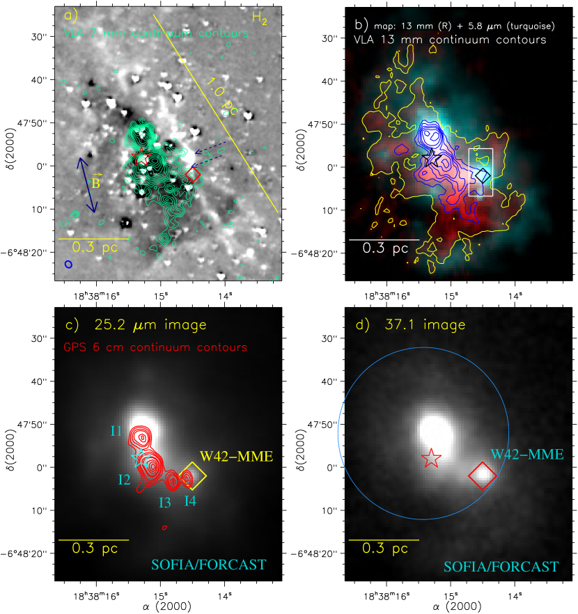
In Figure 1a, we show the overlay of the VLA 7 mm/49 GHz radio continuum emission contours on the H2 image, showing the wide-scale environment of W42-MME. In the background map, the parsec scale H2 outflow with H2 knots/bow-shock feature is evident. In the immediate vicinity of the 6.7 GHz MME, at least two H2 knots are indicated by arrows. Note that the continuum and line data (from VLA/SMA/ALMA) used in this paper do not cover the area containing the entire parsec scale H2 outflow.
In Figure 1b, we overlay the VLA 13 mm/23 GHz radio continuum emission contours on a two color-composite map (VLA 13 mm (red) and Spitzer 5.8 m (turquoise) images) of W42. The VLA 13 mm continuum emission is distributed well within an emission structure seen in the Spitzer 5.8 m image. Earlier, this structure was reported as an ionized cavity-like feature using the H2 emission, the Spitzer 5.8 m image, and the radio continuum emission (see Figure 2a in Dewangan et al., 2015a).
Figures 1c and 1d show the SOFIA 25.2 m and 37.1 m continuum images, respectively. We also observe the MYSO W42-MME in both the SOFIA infrared images. The observed NIR emission from the protostars is mainly due to scattered light escaping from the cavities (e.g., Zhang & Tan, 2011), whereas the observed mid-infrared emission can be explained as thermal emission from warm dust in the outflow cavity walls. In Figure 1c, we also display the GPS 6 cm Epoch 3 radio continuum contours overlaid on the SOFIA continuum image at 25.2 m. Using the clumpfind IDL program (Williams et al., 1994), four ionized clumps are identified in the GPS 6 cm continuum map, and are labeled as I1, I2, I3, and I4 in Figure 1c. In addition to the total flux, the clumpfind also gives the full width at half maximum (FWHM) not corrected for beam size for the x-axis (i.e., FWHMx), and for the y-axis (i.e., FWHMy). The total fluxes (FWHMx FWHMy) of the ionized clumps I1, I2, I3, and I4 are about 32.7 mJy (3.′′3 2.′′9), 74.4 mJy (3.′′9 3.′′0), 17.8 mJy (2.′′6 1.′′9), and 7.9 mJy (2.′′2 1.′′4) mJy, respectively. We also computed the total fluxes of I1(I2) at 13 mm and 7 mm to be 300(400) mJy and 170(270) mJy, respectively (see Figures 1a and 1b). On the basis of the spectral index calculation between 6 cm and 13 mm, the sources I1 and I2 are optically thick at 6 cm.
On the other hand, no emission is detected toward the ionized clumps I3 and I4 in the maps at 13 and 7 mm. Hence, we estimated upper limits on fluxes of I3(I4) to be of 22(17) mJy and 17(15) mJy at 13 mm and 7 mm, respectively. These estimates take into account inhomogeneities of the diffuse emission observed toward the area hosting these sources. Concerning the sources I3 and I4, these estimates are in agreement with optically thin emission from 6 cm to 7 mm. Following Dewangan (2021), we compute the number of Lyman continuum photons of only two ionized clumps, I3 and I4 (see also Matsakis et al., 1976), which seem to be optically thin at 6 cm. The calculation uses the observed flux values, electron temperature = 10000 K and distance = 3.8 kpc. We determined of I3 and I4 to be 46.4 and 46.0 s-1, respectively. Using the reference of Panagia (1973), both these ionized clumps are powered by a massive B-type star. Note that the ionized clump I4 is traced near the position of W42-MME, which has an offset of about 1.′′4. However, the VLA 7 mm and 13 mm continuum maps do not show any radio counterpart of W42-MME.
Noticeable radio continuum emission is observed around a region containing the position of the O5-O6 star in the observed 6 cm, 7 mm, and 13 mm continuum maps (see the ionized clumps I1 and I2), where the infrared emission is also detected in the SOFIA images at 25.2 and 37.1 m (see Figure 1). As per our calculations, we find that the sources I1 and I2 are optically thin at 13 mm (23 GHz). Hence, using the observed fluxes at 13 mm, we estimate of the ionized clumps I1 and I2 to be 47.6 and 47.8 s-1, respectively. Following Panagia (1973), both these ionized clumps are excited by a massive B0V-O9.5V star. However, a detailed study of I1 and I2 is beyond the scope of this paper. This work mainly focuses around W42-MME.
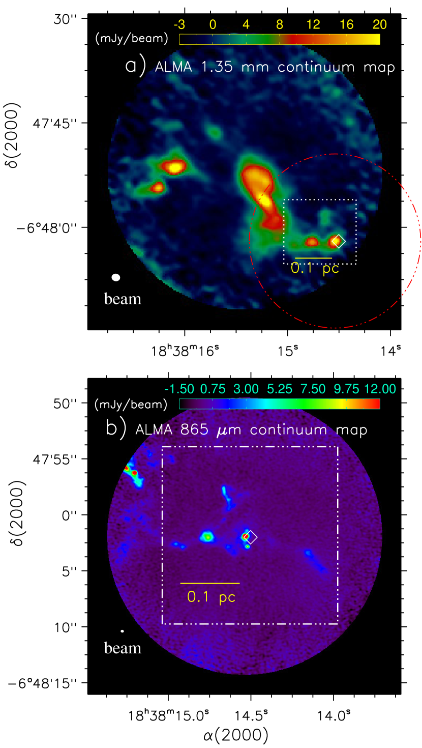
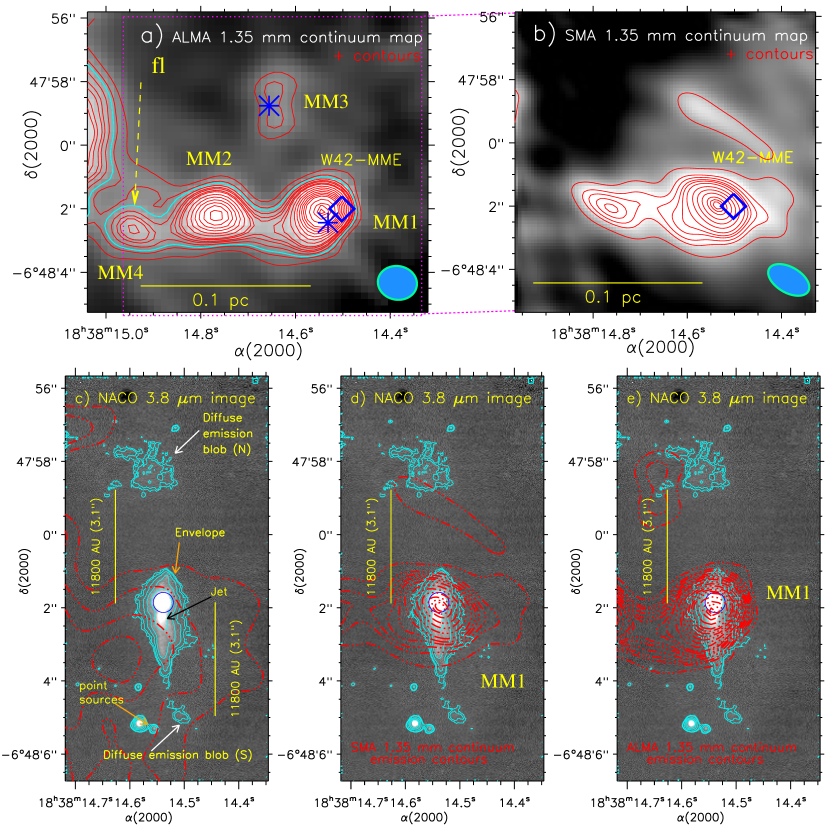
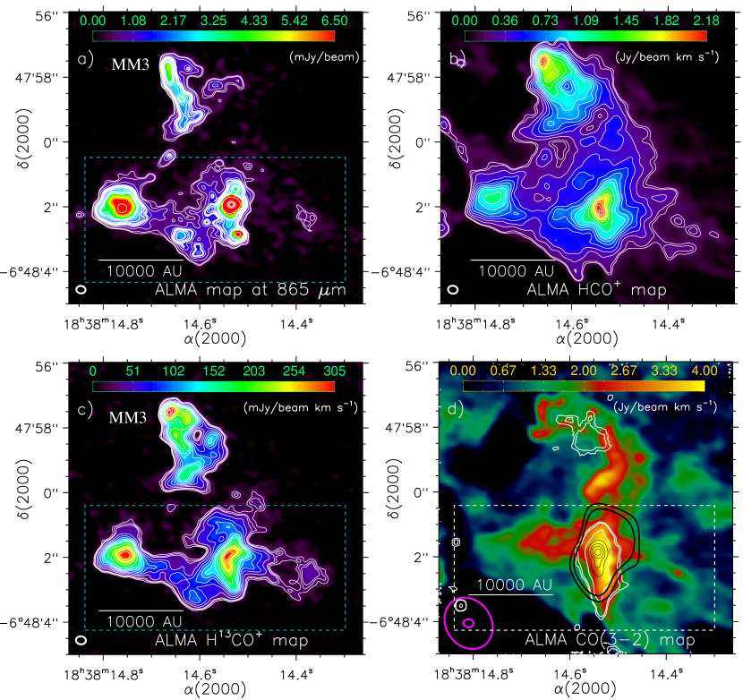
Figure 2a displays the ALMA band-6 (1.35 mm) continuum map (beam size 1.′′2 1.′′1) of W42, and the field of view of this observation is indicated by a big circle (radius 20′′) in Figure 1d. In Figure 2b, we present the ALMA band-7 (865 m) continuum map (beam size 0.′′29 0.′′23 or 1100 AU 875 AU) of W42-MME. A dotted-dashed circle (radius 12.′′5) outlines the field of view of the band-7 observation in Figure 2a. A detailed examination of the ALMA band-7 continuum map is presented in Section 3.1.3. Figures 3a and 3b display zoomed-in views of the ALMA band-6 and SMA continuum maps at 1.35 mm of W42-MME, respectively. Both the maps have a beam size of 1′′. The ALMA band-6 continuum map reveals three compact mm sources (i.e., MM1, MM2, and MM4) as well as one more mm continuum source MM3, which does not appear as a compact object. The three continuum sources MM1, MM2, and MM4 appear to coincide with a diffuse, elongated feature (“fl”; extent 0.15 pc) in the ALMA band-6 continuum map (see the cyan contour at 5.153 mJy beam-1 in Figure 3a). The two sources (i.e., MM1 and MM2) are spatially seen over a scale of 0.1 pc in the SMA continuum map, and are found near the ionized clumps (i.e., I4 and I3; see Figure 1c). The other two continuum sources (i.e., MM3 and MM4) do not coincide with the radio continuum peaks traced in the GPS continuum map at 6 cm.
In Figures 3c, 3d, and 3e, we present the VLT/NACO L′ image overlaid with the continuum emission contours at VLA 7 mm, SMA 1.35 mm, and ALMA 1.35 mm, respectively. In these figures, the contours of L′ image are also presented to display the diffuse infrared emission, the proposed infrared jet, and the outflow cavity/infrared envelope. A small circle is also marked to highlight the position of the powering source of the infrared outflow/jet. The jet-outflow W42-MME system is embedded within the compact source MM1. The mm continuum source MM3 appears to be associated with the diffuse infrared emission traced in the L′ image, where the H2 emission is also detected (see an arrow in Figure 1b). Furthermore, the position of a water maser (from Walsh et al., 2014) is also observed toward the sources MM1 and MM3 (see asterisks in Figure 3a).
3.1.2 Determination of the mass of mm continuum sources
The mass of each compact continuum source is estimated with the knowledge of its integrated flux and temperature. In this relation, we employed the clumpfind IDL program to compute the integrated fluxes at ALMA 1.35 mm of the continuum sources. We examined the Herschel temperature () map to obtain the dust temperature toward W42-MME, which is found to be 40 K. The mass of the mm continuum source was computed using the following formula (Hildebrand, 1983):
| (1) |
where is the integrated 1.35 mm flux (in Jy), is the distance (in kpc), is the gas-to-dust mass ratio (assumed to be 100), is the Planck function for a dust temperature , and is the dust absorption coefficient. Here, we used = 0.9 cm2 g-1 at 1.3 mm (Ossenkopf & Henning, 1994), = 3.8 kpc, and = 40 K. The flux densities (FWHMx FWHMy) of the compact continuum sources MM1, MM2, and MM4 in continuum are about 36.0 mJy (1.′′49 1.′′23), 26.6 mJy (1.′′59 0.′′99), and 7.7 mJy (1.′′25 0.′′63), respectively. The masses of MM1, MM2, and MM4 are estimated to be 5.2, 3.9, and 1.1 M⊙, respectively. If we use = 70 K (see Section 3.3.1) then the masses of MM1, MM2, and MM4 are computed to be 2.8, 2.1, and 0.6 M⊙, respectively. As mentioned earlier, the ionized clump I4 overlaps with the source MM1 at 1.35 mm. Hence, free-free emission from I4 can contribute to the mm flux of MM1. We computed this contribution from the 6 cm flux assuming the spectral index of 0.1 typical for optically thin free-free emission. In this way, we obtain the upper limit for this contribution of 5.4 mJy, which is about 15% of the derived flux value of 36.0 mJy. On the basis of the corrected flux value (i.e., 30.6 mJy), the mass of MM1 is determined to be 4.4(2.4) M⊙ at = 40(70) K. In the case of MM2 and MM4, we are unable to estimate a possible free-free contribution. In general, the estimation of the mass suffers from various uncertainties, which include the assumed dust temperature, opacity, and measured flux. Hence, the uncertainty in the mass estimate of each continuum source could be typically 20% and at largest 50%.
We also computed the total mass of the elongated feature “fl” (extent 0.15 pc) to be 11.2 M⊙ at = 40 K. This estimation uses the integrated flux of the elongated feature (i.e., 77.4 mJy), which was determined using the clumpfind IDL program. If we treat this feature as a filament having a high aspect ratio (length/diameter) then its line mass, or mass per unit length (i.e., Mline,obs) is determined to be 75 M⊙ pc-1. One can define a critical line mass Mline,crit for a gas filament, modeled as an infinitely long, self-gravitating, isothermal cylinder without magnetic support, given by M M⊙ pc (e.g., Ostriker, 1964; Inutsuka & Miyama, 1997; André et al., 2014). Our value of 75 M⊙ pc-1 suggests that the feature “fl” is a thermally supercritical filament. It is thought that thermally supercritical filaments are prone to radial gravitational collapse and fragmentation (e.g., André et al., 2010). In general, a factor of “” is involved in the estimate of the line mass of a filament (i.e., Kainulainen et al., 2016), where ”i” is the angle between the sky plane and the filament’s major axis. Here, we consider the filament lying in the sky plane, resulting in “ = 1”.
3.1.3 ALMA sub-mm continuum map
The continuum emission of MM1 at 1.35 mm may arise from the dusty envelope and disc surrounding the MYSO W42-MME. However, the resolution of the ALMA band-6 and SMA continuum maps at 1.35 mm (1′′) is not enough to further resolve the disk or the inner circumstellar substructures of MM1 (see Figures 2a and 2b).
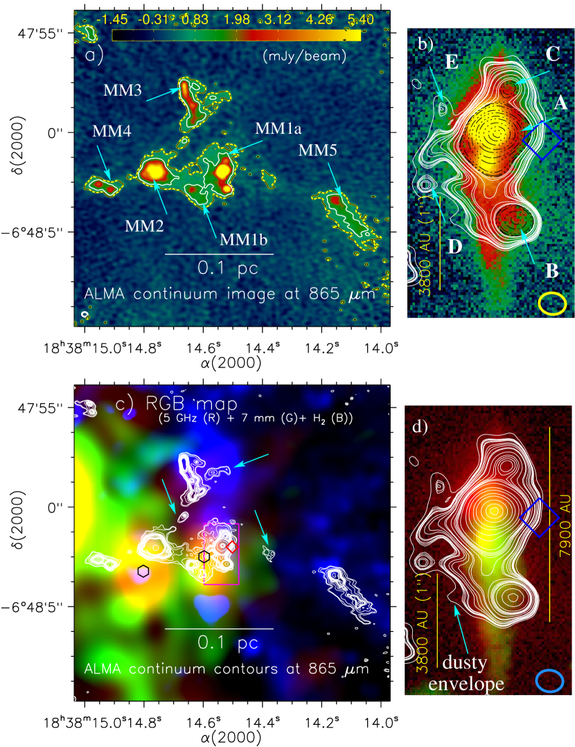
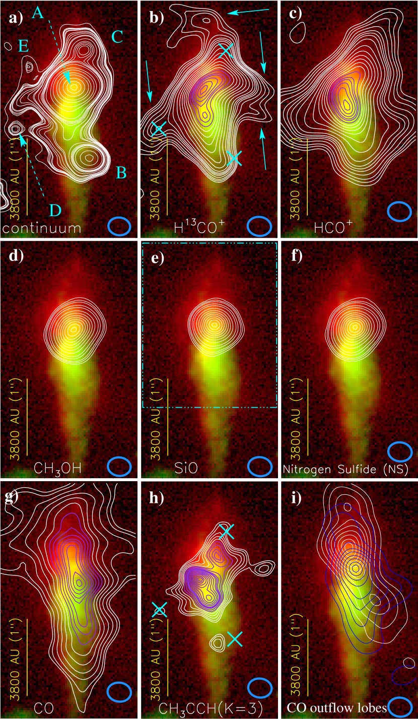
In Figure 4a, we present the ALMA continuum map at 865 m, where a broken contour at 0.45 mJy beam-1 (3) is drawn to indicate the extent of the continuum emission. The 865 m continuum contour (in white) at 1.1 mJy beam-1 is also overlaid on the map, tracing the six distinct cores (MM1a, MM1b, MM2–5). The source MM1a is seen toward MM1, while the source MM1b is detected between MM1 and MM2. Note that the core MM5 is located outside the 1.35 mm map area of Figures 3a–3b. The 865 m color scale shows that at the higher frequency and resolution of the ALMA band 7 observations, the mm cores lying along the filament have internal structure with multiple components.
Figure 4c shows a three color-composite map (GPS 5 GHz/6 cm (red), 7 mm (green), and H2 (blue) images) overlaid with the ALMA continuum emission contours at 865 m. The color-composite map shows that none of the mm sources MM1–5 coincide with the radio continuum peaks (see black hexagons). Arrows indicate three additional continuum sources that were not detected at 1.35 mm.
The NACO L′ image around MM1a is presented in Figure 4b, while a two-color composite NACO image (L′(red) + Ks (green)) around MM1a is displayed in Figure 4d. The NACO color-composite map is taken from Dewangan et al. (2015a). The position of the 6.7 GHz MME is indicated by a diamond symbol in Figures 4b–4d. The infrared envelope/outflow cavity, the powering source of the H2 outflow, and the proposed infrared jet are brighter in the L′ image than the Ks image. The diffuse emission observed in the Ks image coincides well with the jet-like feature, which has been suggested as an ionized jet (see Dewangan et al., 2015a, for more details).
In Figures 4b and 4d, the ALMA continuum emission contours at 865 m are also shown, revealing the substructure of the western part of core MM1. The inner circumstellar structure of W42-MME traced in the NACO images and the ALMA continuum map can be compared in these figures, showing a dusty or circumstellar envelope (extent 7900 AU) surrounding the MYSO W42-MME (see an outer contour in Figures 4b and 4d). The ALMA continuum map further reveals five continuum peaks “A–E” inside the dusty envelope. Two of these, “A” and “B”, are resolved by the ALMA beam. Furthermore, the previously reported infrared envelope/outflow cavity is also seen toward the dusty envelope. The peak flux density (Rayleigh-Jeans temperature or radiation temperature) of A, B, C, D, and E is found to be 4.36 mJy beam-1 (6.5 K), 0.94 mJy beam-1 (1.4 K), 0.39 mJy beam-1 (0.58 K), 0.15 mJy beam-1 (0.23 K), and 0.14 mJy beam-1 (0.21 K), respectively. Here, a conversion factor between flux density and radiation temperature for the ALMA beam is 150 K Jy-1 (see also Zinchenko et al., 2020). The ALMA continuum source “A” hosts the powering source of the H2 outflow and the proposed infrared jet. The H2 knots are seen to the north of source “A” (Figure 4c). The other continuum peaks/sources “B–E” are in the immediate surroundings of the continuum source “A” within the dusty envelope.
The detection of MM1 in the maps at 1.35 mm and 865 m enables us to estimate its spectral index, which is found to be about 3.6, favoring an optically thin dust emission. This calculation includes the correction for the I4 contribution. In the case of MM2, the spectral index between 1.35 mm and 865 m is determined to be 3. Mass estimates from the 865 m continuum map should be more reliable because the relative contribution of the free-free emission at this wavelength is much lower than at 1.35 mm.
Using Equation 1, we also computed the masses of six continuum sources (i.e., MM1a, MM1b, MM2, MM3, MM4, and MM5) detected in the ALMA map at 865 m. It is noted that the sources “A–E” are seen in the direction of the continuum source MM1a. Table 2 contains physical parameters (i.e., position, flux density, FWHMx FWHMy, and mass) of six continuum sources. The integrated fluxes at 865 m were obtained using the clumpfind IDL program. In the calculations, we used = 1.85 cm2 g-1 at 865 m (Schuller et al., 2009), = 3.8 kpc, and = [40, 70] K. The mass of the source “A” is also estimated to be 2.2 and 1.2 M⊙ at = 40 and 70 K, respectively. Here, the flux density (FWHMx FWHMy) of the continuum source “A” is determined to be 71.8 mJy (0.′′35 0.′′35).
3.2. Molecular Line Emission
Several molecular lines are detected toward our target source, and are observed by the SMA, VLA, ALMA band-6 and ALMA band-7 facilities. In the direction of W42-MME, the molecular emission is mainly studied in a velocity range of [60, 70] km s-1.
3.2.1 Molecular Lines from the SMA and VLA
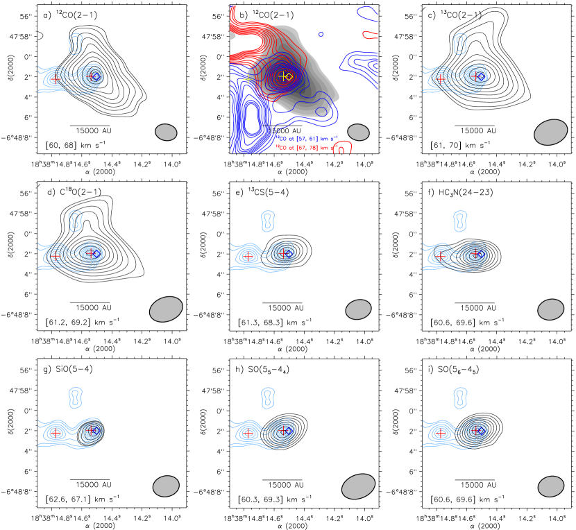
In Figures 5 and 6 we present the integrated intensity maps of different molecular emission (spatial resolution 1′′–3.′′5) traced by the SMA and VLA. We do not detect any NH3 or SiO(1–0) emission with the VLA. Only one line (i.e., CS(1–0)) from the VLA is presented in this work.
The lines detected by the SMA facility are CO(2–1), 13CO(2–1), C18O(2–1), 13CS(5–4), HC3N(24–23), SiO(5–4), SO(55–44), SO(56–45), CH3CN(121–111), CH3CN(120–110), CH3OH(51,4–42,2), H2CO(30,3–20,2), H2CO(32,2–22,1), and H2CO(32,1–22,0). We find compact emission coincident with MM1 in many molecular species. The SMA detected dense/hot gas tracers CH3CN, CH3OH, HC3N, 13CS, shock tracer SiO, two SO transitions, and H2CO. The detections of different sub-mm molecular lines suggest the presence of a hot molecular core associated with W42-MME. The analysis of the gas temperature of MM1 is presented in Section 3.3.
The maps of three CO isotopologues 12CO, 13CO, and C18O are presented in Figures 5a, 5c, and 5d, respectively. Figure 5b shows a molecular outflow traced using the CO(2–1) line; the outflow is centered at the continuum peak MM1. We find a very compact morphology of the shock tracer SiO in the direction of continuum source MM1 (see Figure 5g), indicating the presence of shocked gas. However, in other outflow tracers (e.g., CO, SO, CS), the emission is slightly more extended than in SiO, suggesting that the ambient gas might have been entrained by the outflow/jet from W42-MME.
Using the VLA, we detected the CS(1–0) line, which is presented in Figure 6g. The CS(1–0) emission contours are overlaid on the ALMA continuum map at 865 m (see Figure 6h), and appear to enclose the dusty envelope (see also Figure 4d). Figure 6i displays the overlay of the SMA H2CO(30,3–20,2) emission contours on the ALMA continuum map at 865 m, showing all six ALMA continuum sources distributed within the extended H2CO emission.
3.2.2 Molecular Lines from ALMA band-7
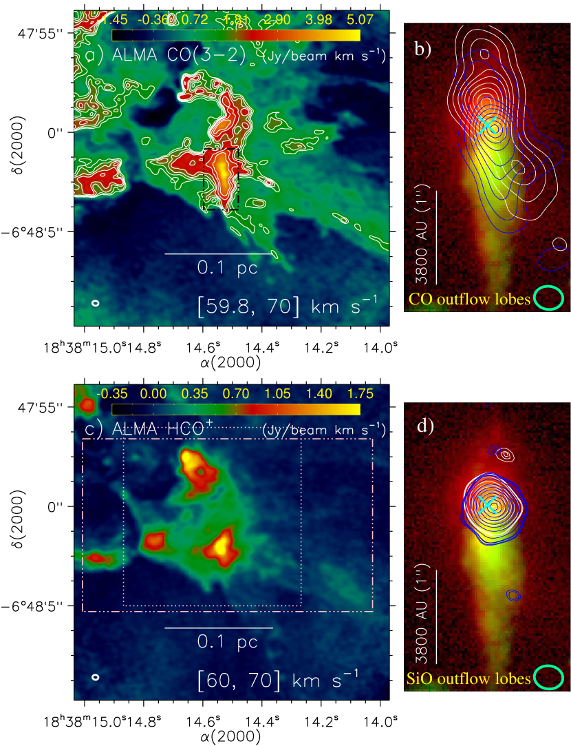
In this section we examine CO(3–2), HCO+(4–3), H13CO+(4–3), and SiO(8–7) lines from the ALMA band-7. In Figures 7a, 7c, and 8a, we display the integrated intensity maps of the CO(3–2), HCO+, and H13CO+ emission (resolution 0.′′3) of an area around W42-MME, respectively. A comparison of the morphology of the integrated line emission with the dust shows a similar appearance, suggesting that these line data can be utilized to study motions of the circumstellar materials around W42-MME. Such a study cannot be done using the SMA, ALMA band-6, or VLA data, which have relatively lower resolution (i.e., 1′′–3.′′5; C.F. Table 1). The H13CO+ line traces denser regions compared to the CO(3–2) and HCO+ lines.
Figures 7b and 7d show the overlay of the CO(3–2) and SiO(8–7) outflow lobes on a two-color composite NACO image (L′(red) + Ks (green)) around MM1a, respectively. The CO outflow lobes are studied in velocity ranges of [30, 54] and [75, 104] km s-1, while the SiO outflow lobes are shown in velocity ranges of [40, 55] and [73, 90] km s-1. Both the molecular outflows are centered at the continuum source “A” (see a multiplication symbol in Figures 7b and 7d). The SiO outflow lobes are spatially concentrated toward source “A”. The SiO outflow lobes are more compact (extent 3500 AU) than the CO outflow lobes (extent 9000 AU). It seems that the CO outflow is in the plane of the sky, while the SiO outflow is to the plane of the sky. Furthermore, the spatial extent of the CO outflow lobes also hints the outflow cavity walls, which might also be outlined by the VLA CS emission.
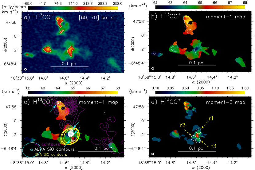
In the maps of the HCO+ and H13CO+ emission, the molecular gas toward the continuum sources (MM1a, MM1b, MM2, MM3, MM4, and MM5) is seen. The highest intensity is found toward the continuum source MM3 which shows a bow-like appearance. Figure 8b presents the moment-1 map of the H13CO+ emission, showing the intensity-weighted mean velocity of the emitting gas. The gas associated with the continuum source MM3 appears redshifted with respect to other continuum sources. A noticeable velocity difference can also be seen toward the continuum source MM1a (see the H13CO+ emission contour in Figure 8b). In Figure 8c, we present the overlay of the contours of the SMA SiO(5–4), ALMA SiO(8–7), and H2 emission on the H13CO+ moment-1 map. The emission peak of the SMA SiO(5–4) is detected toward the continuum source MM1a. However, the ALMA SiO(8–7) emission at [60.8, 71] km s-1 is seen toward the continuum sources “A–C” and the H2 knot (see arrows in Figure 8c). The dusty envelope as well as continuum peaks appear to be influenced (i.e., heated) by shocks. Therefore, using the continuum map, mass estimations of the continuum sources distributed within the source MM1a may not be accurate. Furthermore, the SiO(8–7) emission is also detected in the direction of the tip of the bow-like appearance of the continuum source MM3, where the H2 knot is seen. Figure 8d displays the moment-2 map or the intensity-weighted dispersion map of the H13CO+ emission. In the direction of the continuum sources MM1, MM2, and MM3, we find a velocity dispersion larger than 1 km s-1. The velocity dispersion toward the source “A” may be related to rotation (see also Section 4.2).
In Figure 9a, we show the ALMA continuum map and contours at 865 m toward an area containing the mm continuum sources MM1–3. Figures 9b and 9c display the integrated intensity maps and contours of the HCO+ and H13CO+ emission at [60, 70] km s-1, respectively. In Figure 9d, we present the integrated intensity map of the CO(3–2) emission at [59.8, 70] km s-1 and the NACO L′ emission contours. The VLA CS(1–0) emission contours (in black) are also shown in Figure 9d. We find strong intensity of the molecular emission toward the continuum source “A” and the dusty envelope. The spatial morphology of the continuum source “A” and the dusty envelope look little different in the VLT/NACO L′ image, and the emission maps of CO(3–2), H13CO+, and HCO+ (see Figure 9 and also Section 3.4).
The 865 m continuum map and the H13CO+ emission map exhibit a similar morphology, where an emission feature (extent 0.1 pc) hosting the continuum sources MM1a, MM1b, and MM2 is evident (see the dotted box in Figures 9a and 9c). As mentioned earlier, the continuum source MM3 is very prominent in the continuum map and the integrated line maps of the H13CO+ and HCO+ emission, and is associated with the shock-excited molecular line emission resulting from the W42-MME jet/outflow activity (see Figure 8c). Note that the location of MM3 is far away from the extent of the ALMA CO outflow lobes. More discussion on these findings is given in Section 4.
3.3. Gas temperature and non-thermal dispersion
3.3.1 Gas temperature
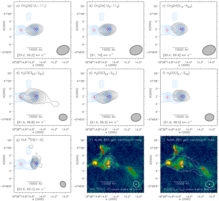
In this section, the lines methyl cyanide/acetonitrile/cyanomethane, CH3CN from ALMA band-6 and propyne/methyl acetylene, CH3CCH from ALMA band-7 are explored for obtaining the gas temperature of the core MM1 or the continuum source “A”.
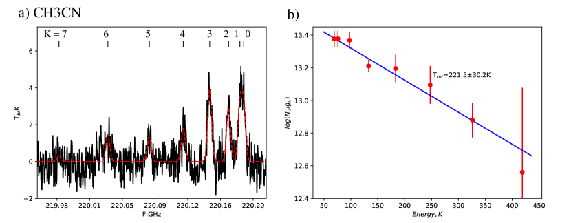
We examined several transitions of the CH3CN emission observed in ALMA band-6 (resolution 1′′). Eight components of the CH3CN -ladder with =0-7 are observed, and their spectra are presented in Figure 10a. These transitions have been used to determine the rotational temperature at the location of the continuum peak MM1. In Figure 10a, all CH3CN transitions are simultaneously fitted by a model given in Araya et al. (2005). The model assumes local thermodynamic equilibrium (LTE) conditions. In Figure 10b, we present the CH3CN rotation diagram of the continuum source MM1. The best fit yields a rotational temperature, , of 221.530.2 K. The uncertainty in the CH3CN temperature is 3. Using the different transitions of the SMA CH3CN line (resolution 3′′), we derive a rotational temperature of 152 K.
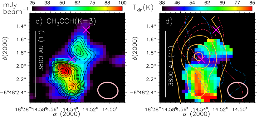
Five components of the CH3CCH emission (beam size 0.′′3 0.′′24) are detected in the ALMA band-7. These data have a better spatial resolution compared to the SMA/ALMA CH3CN data. In Figure 10c, we present the integrated intensity map and contours of the CH3CCH ( =3 transition) emission around the continuum source “A”. The kinetic temperature of the CH3CCH gas is determined by the method of population diagrams (see Malafeev et al., 2005, for more details). Figure 10d displays the kinetic temperature map around the source “A”. The temperature map is also overlaid with the ALMA CO outflow direction (i.e., NE–SW) and the NACO L′ emission contours. The locations of the continuum sources “A” and “C” are marked by multiplication symbols in the map. The range of the gas temperature is determined to be [38, 85] K. A noticeable gas temperature gradient is evident toward the source “A” or the areas covered by the NACO emission contours, which highlight the proposed ionized jet-like feature and the location of the MYSO. Higher gas temperatures are found toward regions located in the North and SE directions. The proposed ionized jet-like feature is detected with higher gas temperatures (i.e., 60–85 K; mean value 70 K). All these exercises suggest that the core MM1 or MM1a is heated by the MYSO W42-MME. One can also notice a difference in temperature estimates from the CH3CN and CH3CCH emission. It can be explained with the fact that the CH3CN emission is produced from a warmer and inner region of the envelope than the CH3CCH emission (e.g., Andron et al., 2018).
Taking into account the detections of several sub-mm lines and higher gas temperature, our results confirm the presence of a hot molecular core associated with the MYSO W42-MME.
3.3.2 Non-thermal dispersion and signature of infall motion
Using the optically thin H13CO+ line, we examined the spectra toward three small regions (i.e., r1, r2, and r3) around the continuum source “A” (see circles in Figure 8d), and computed the FWHM linewidth of each observed H13CO+ profile (not shown here). Using the observed FWHM value, we determined the sound speed (), thermal velocity dispersion (), non-thermal velocity dispersion (), Mach number ( = /), and ratio of thermal to non-thermal gas pressure ( = ; see Lada et al., 2003, for more details). The sound speed ( = ) is estimated for = 2.37 (approximately 70% H and 28% He by mass) and a range of temperature (i.e., = [40, 70] K). The non-thermal velocity dispersion is defined as:
| (2) |
where is the measured linewidth of the observed H13CO+ profile, (= ) is the thermal broadening for H13CO+. In the direction of regions r1, r2, and r3, the value of non-thermal velocity dispersion is determined to be 0.92(0.91), 0.93(0.92), and 1.0(1.0) km s-1 at = 40(70) K, respectively. Using the value of = 40(70) K, we obtain the sound speed to be 0.37(0.49) km s-1 toward the regions r1, r2, and r3. In the direction of the regions r1, r2, and r3, the Mach number is estimated to be 2.5(1.9), 2.5(1.9), and 2.8(2.1) at = 40(70) K, respectively. For the value of = 40(70) K, the is estimated to be 0.16(0.29), 0.16(0.28), and 0.12(0.22) toward the regions r1, r2, and r3, respectively. Based on these derived physical parameters, we suggest that non-thermal pressure and supersonic non-thermal motions (e.g., turbulence, outflows, shocks, and/or magnetic fields) are dominant in these regions, which are not exactly coincident with the continuum source “A” (see circles in Figure 8d).
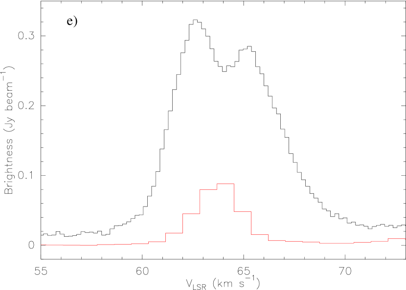
In Figure 10e, we present the profiles of the H13CO+(4–3) emission (in red) and HCO+(4–3) emission (in black) toward the continuum source “A”. A single peak is seen in the optically thin H13CO+ line, while a red-shifted self-absorption dip is detected in the optically thick HCO+ line at the W42-MME position. These profiles may indicate the signatures of infall toward the continuum source “A”, although this is not certain since the HCO+ profile varies significantly across the source, which can be caused by a complicated morphology of the HCO+ distribution.
3.4. Multiline spectral imaging view of continuum source MM1a
In the direction of the continuum source MM1a, in Figures 11a–11i, we present a zoomed-in view of a two-color composite NACO map (L′ (red) and Ks (green) images) overlaid with the emission contours of the 865 m continuum, H13CO+(4–3), HCO+(4–3), CH3OH, SiO(8–7), nitrogen sulfide (NS), CO(3–2), CH3CCH (k=3), and CO outflow lobes, respectively. Some of these lines (i.e., H13CO+, CH3OH, and NS) are known as dense gas tracers. Figures 11a, 11e, and 11i are the same as presented in Figures 4d, 8c, and 7b, respectively, which are shown here only for a comparison purpose.
In Figure 11a, the continuum source “A” is seen almost at the center of the dusty envelope, and is surrounded by four continuum peaks “B–E”. In the direction of the proposed infrared envelope/outflow cavity, the outflow cavity walls are depicted by the CO emission and the CO outflow lobes (see Figures 11g and 11i). The outer contours of the H13CO+ and HCO+ emission display narrow molecular structures (see arrows in Figure 11b), which may show the outflow cavity walls (see Figures 11b and 11c). In Figure 11b, multiplication symbols (in cyan) show the locations of the continuum sources (i.e., B, C, and D), which are interestingly seen toward narrow structures of the H13CO+ emission.
The continuum source “A” is well traced in the shock gas tracer SiO(8–7) and the dense gas tracers NS and CH3OH. The spatial morphology of the continuum source “A” appears similar in the maps of the CH3OH, SiO(8–7), and NS emission. Note that the ALMA SiO data also reveal the compact SiO outflow concentrated toward the source “A” (see Figure 7d).
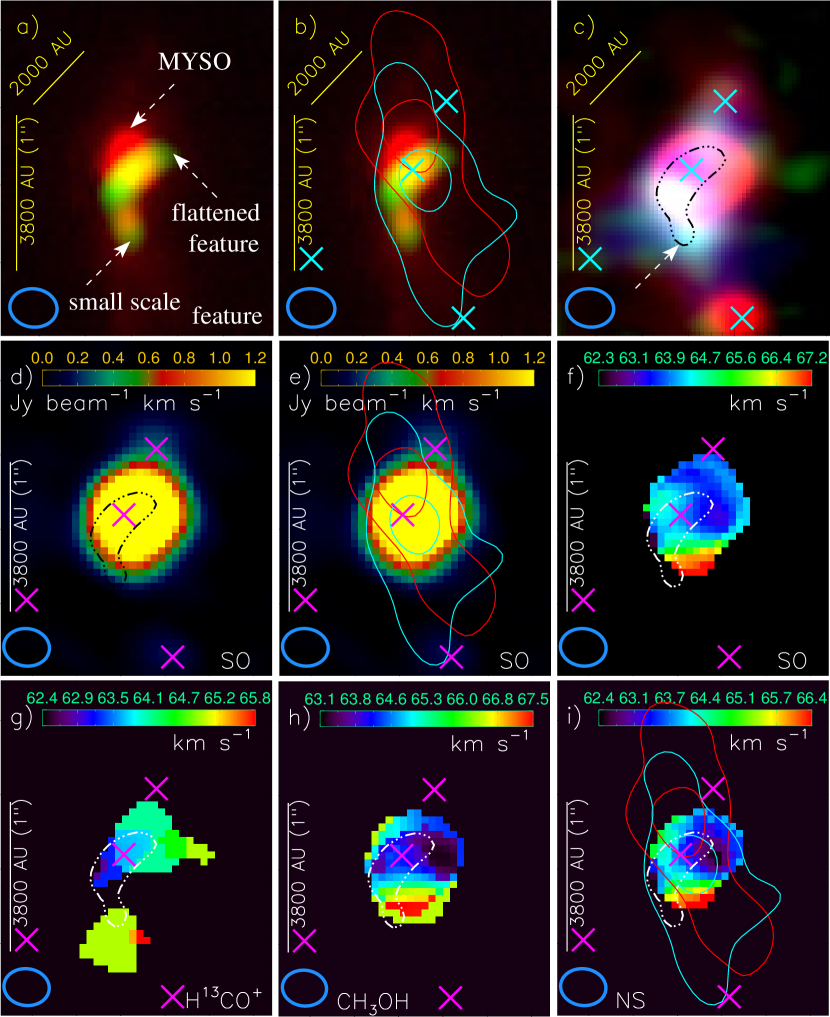
The H13CO+, HCO+, CO, and CH3CCH emission contours with higher intensities are shown by magenta color, and are seen toward the continuum source “A”. The peak of the CH3CCH emission ( = 3 component) lies slightly to the south of “A” and peaks toward the proposed infrared jet-like feature. The H13CO+ emission contours are distributed in the northwest to southeast direction, appearing like a flattened/elongated feature.
In Figure 12a, we display a two color-composite map (NACO L′ band (red) + H13CO+ (green)) toward an area containing the continuum sources “A–D” (see a dotted-dashed box in Figure 11e), strongly showing the flattened/elongated feature (extent 2000 AU) in the H13CO+ emission. The MYSO W42-MME is almost seen at the center of the flattened feature. Figure 12b is the same as Figure 12a, but the color-composite map is overlaid with the CO outflow lobes. The peak positions of the continuum sources (A–D) are also shown in Figure 12b.
The elongation of the H13CO+ emission hints that the feature is located at a large inclination. The orientation of the CO outflow lobes is also perpendicular to the H13CO+ flattened feature (see Figure 12b). It has been suggested that outflows/jets are always launched perpendicular to the disk plane (Monin et al., 2007). Hence, the flattened feature could be an accretion disk-like feature around the MYSO W42-MME. Figure 12c displays a three color-composite image (ALMA continuum map at 865 m (red) + CH3CCH (green) + HCO+ (blue)) overlaid with the H13CO+ emission, illustrating the association of the H13CO+ flattened feature with the continuum emission and HCO+. However, the flattened/elongation morphology is not seen in the continuum map. In Figures 12d and 12e, we present the moment-0 map of the Sulphur monoxide (SO) 8(8)–7(7) emission. We trace very strong SO emission toward W42-MME using the SMA facility, and it is also very strong in the ALMA data having a higher resolution. The flattened feature is highlighted in Figure 12d, and the CO outflow lobes are displayed in Figure 12e. In the direction of the proposed infrared jet-like feature, we also detect the noticeable H13CO+, CH3CCH ( =3 transition), and HCO+ emission, which is referred to as a small-scale feature. The small-scale feature is not located in the direction of the ALMA CO outflow lobes, suggesting that it is unlikely to be a jet. In the maps of the continuum, CH3OH, SO, and SiO emission, no peak is seen toward the small-scale feature (see also Figures 11a, 11d, and 11e). The implication of the observed flattened feature and small-scale structure for the formation of the O-type star is discussed in Section 4.
4. Discussion
The present paper deals with a young O-type protostar W42-MME (mass: 194 M⊙; luminosity 4.5 104 L⊙). W42-MME is saturated in the Spitzer 8.0 and 24.0 m images, and appears as a point-like source in the SOFIA images at 25.2 and 37.1 m (see Section 3.1). Dewangan et al. (2015a) reported a parsec-scale H2 outflow driven by this object, and employed the high resolution NIR data (resolution 0.′′1–0.′′2) to study its inner circumstellar environment. These data sets allowed them to investigate an infrared envelope/outflow cavity (extent 10640 AU), which surrounds the O-type star and an ionized jet-like feature. In this paper, we aim to understand the physical process of mass accumulation in the formation of this young O-type star. Hence, the findings of Dewangan et al. (2015a) are used as a basis for further exploring the complex circumstellar environment of the MYSO W42-MME using high resolution (0.′′3–3.′′5) continuum and spectral line data observed in the sub-mm, mm, and cm regimes.
The ionized clump I4 is found to be close to the position of W42-MME (see Figure 2c), but new VLA 7 and 13 mm continuum maps do not detect any radio counterpart of the MYSO W42-MME (see Section 3.1). Based on the NIR polarimetric data, the H2 outflow axis is parallel to the magnetic field at the position angle of 15 (see Figure 1a).
The hot molecular core hosting W42-MME (i.e., MM1) is investigated using the SMA and ALMA molecular line data (see Section 3.2), and is traced with the gas temperature of 38–221 K (see Section 3.3.1). The SMA and ALMA molecular line data also confirm that W42-MME drives a molecular outflow. The ALMA 1.35 mm continuum map shows the presence of an elongated and thermally supercritical filament-like feature (extent 0.15 pc) containing at least three continuum cores (mass range 1–4.4 M⊙) including MM1 (see Section 3.1). The elongated filament-feature is also seen in the ALMA continuum map at 865 m. As seen in Figures 4a and 4b, the ALMA 865 m continuum map resolves MM1 into at least two continuum sources MM1a and MM1b. In the direction of MM1a, at least five continuum sources/peaks (“A–E”) are traced within the dusty envelope (extent 9000 AU), where shocks are investigated in the SiO(8–7) emission. The continuum source “A” associated with W42-MME is found almost at the center of the dusty envelope, and is surrounded by other continuum peaks (“B–E”). A disk-like feature and a small-scale feature are identified toward “A” using multi-wavelength data (see Section 3.4). A variation in the gas temperature (i.e., 38–85 K) toward these features is found in the kinetic temperature map derived using the ALMA CH3CCH lines.
Collectively, these observed features must be interpreted to understand their role in the formation of the O-type star.
4.1. Signature of an episodic accretion process
In general, the observed outflows around protostars suggest a disk-mediated accretion process (Arce et al., 2007). From Figure 8c, one can identify different H2 knots in the northern direction of the H2 outflow, showing the shock activity. We also find the presence of the SiO(8–7) emission toward the knot (see arrows in Figure 8c), indicating that the shocked gas is associated with the energetic outflow. The bipolar structures/lobes centered at W42-MME are traced using the CO(3–2) and SiO(8–7) emission (see Figures 7b and 7d). The most prominent H2 knot is seen toward the continuum source MM3, which does not appear to be part of the elongated filament-like feature. MM3 has a bow-like appearance in the maps of the HCO+(4–3) and H13CO+(4–3) emission, where the diffuse NACO L′ emission is also traced. The HCO+(4–3) and H13CO+(4–3) emissions show the distribution of the quiescent gas around W42-MME. The tip of the bow-like appearance of MM3 is associated with the SiO(8–7) emission (see Section 3.2.2). A water maser is also detected toward MM3, probably showing a signature of shock. Additionally, we do not find any extent of the ALMA CO(3–2) or SiO(8–7) outflow lobes toward MM3.
All these findings suggest the impact of the outflow/jet to the ambient gas around W42-MME, which is an IRc of the 6.7 GHz MME. Recently, flaring methanol masers have been found to trace episodic accretion events in young protostars (e.g., Bertout, 1989; Hirota et al., 2018; Hunter et al., 2018; MacLeod et al., 2018; Chen et al., 2020; Liu et al., 2020; Zinchenko et al., 2020; Stecklum et al., 2021). Hence, our findings appear to show the episodic ejection from W42-MME. Such episodic ejection is presumably driven by accretion events, which are known to occur in such objects (see Hirota et al., 2018; Zinchenko et al., 2020; Liu et al., 2020, and references therein). Together, W42-MME would be a good candidate for monitoring of the methanol (and water) masers in case of a flare.
4.2. Disk-like and small-scale structures around W42-MME
Some theoretical simulations (e.g., McKee & Ostriker, 2003; Krumholz et al., 2009; Hosokawa et al., 2010) predict that massive stars can form through disk mediated accretion upto 140 M⊙ with very high accretion rates (Kuiper et al., 2010, 2013). In addition to the disk-like structure and the outflow cavity, some of the simulations also develop distinct small scale features within a physical scale of about 5000 AU (Smith & Rosen, 2005; Krumholz et al., 2009; Peters et al., 2010a, b; Hennebelle et al., 2011; Hennebelle & Commerçon, 2014). These features can be formed by the gravitational instability, flashlight effect, jet activity, or radiatively driven Rayleigh-Taylor instability around MYSOs.
Concerning the validity of the theoretical predictions, direct observational works of the innermost regions of MYSOs are limited. Some examples of O-type stars having Keplerian-like disks and outflow have been reported in the literature (see Table 1 in Rosen et al., 2020), which are AFGL 4176 (Johnston et al., 2015), G11.92-0.61MM1 (Ilee et al., 2016), G17.64+0.16 (Maud et al., 2018, 2019), and IRAS 16547-4247 (Zapata et al., 2019). These limited cases favour that MYSOs accrete materials via disk-outflow interaction like their low-mass counterparts (e.g. Cesaroni et al., 2007; Zinnecker & Yorke, 2007; Beuther et al., 2009, 2013; Beltrán & de Wit, 2016).
The MYSO W42-MME, associated with the continuum source “A”, drives the molecular outflow traced in the H2, CO, and SiO emission. The self-absorption feature in the HCO+ line profile shows infall toward ”A”. From Figure 12a, the flattened feature and the small-scale structure are evident in the direction of “A”. Both these structures are seen within the dusty envelope/outflow cavity. The ALMA CO outflow lobes are nearly perpendicular to the flattened feature seen in the H13CO+ emission (see Figure 12b). Within a scale of 2000 AU, the point-like source traced in the NACO L′ image is seen at the center of the flattened feature, suggesting that it could be an accretion disk around the MYSO. Figures 12f, 12g, 12h, and 12i show the moment-1 maps of the SO, H13CO+, CH3OH, and NS emission, respectively. The location of the flattened feature is also indicated in each moment-1 map. All these moment-1 maps are clipped at the higher value of the cutoff level. In Figures 12f– 12i, we find a noticeable velocity gradient toward the H13CO+ flattened feature and perpendicular to the outflow. Previously, using the high resolution data (resolution 0.′′5) of the dense gas tracers (e.g., CH3OH and CH3CN), the velocity gradient across the molecular core was suggested as a signature of Keplerian rotation within a rotationally-supported disk (e.g., Zinchenko et al., 2015).
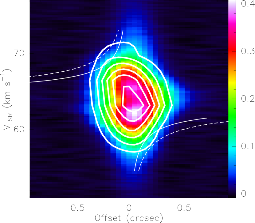
Figure 13 displays the position-velocity diagram along the probable disk in the SO line at the position angle of 132 across the continuum peak “A”. The contours of the CH3OH emission are also shown in Figure 13. The ALMA SO and CH3OH data can help us to better characterize the disk kinematics. The position-velocity diagram enables us to examine the kinematics of the source “A”, and hints the presence of a Keplerian-like rotation of the core “A”. However, the resolution of these data is not sufficient for a reliable conclusion (see also Zinchenko et al., 2020; Liu et al., 2020). Using the rotation velocity information (i.e., ), we compute the dynamical central mass of the core to be 9–12 M⊙. Here, the disk inclination is excluded in the calculation. The dynamical central mass of the core of 12 M⊙ does not properly fit the data (taking into account the angular resolution; see Figure 13), while the value of 9 M⊙ can be treated as an upper limit. As mentioned earlier, the mass of the continuum source “A” is estimated to be 2(1) M⊙ at = 40(70) K. However, we have temperature estimates up to 220 K (see Section 3.3). Hence, this estimated value of 1 M⊙ may show an upper limit of the core mass. Additionally, we examine the shape of the position-velocity diagram, where one can find the broad “waist” feature (see Figure 13). Such features in velocity space suggest infalling motions. More discussion on the broad “waist” feature can be found in Liu et al. (2020, and references therein).
Based on our analysis, we propose two possibilities: 1. To assume that the disk is seen almost face-on. However this contradicts the observed elongation in HCO+/H13CO+. But as mentioned, there is no visible elongation in the continuum. We can assume an asymmetry in the HCO+ distribution in the disk, so that we see only a half of the disk in these lines. Such an assumption is weaker of course but not fully excluded. Another, more natural assumption can be that the bright HCO+ emission is related to the cavity walls and does not directly trace the disk. 2. To assume that we have here a similar situation to that in S255IR-SMA1, where we see a sub-Keplerian rotation accompanied by infall (Liu et al., 2020).
The proposed infrared jet-like feature is referred to as a small-scale feature, and is very well-traced in the H13CO+, CH3CCH ( =3 component), and HCO+ emission (see Figures 12a and 12c). Based on the photometric analysis of the NACO NIR images, it was characterized as an ionized jet-like feature. However, it does not follow the orientation of the ALMA CO outflow, indicating that it is unlikely to be a jet. It is seen toward the continuum source “A”. However, there is no peak of the continuum emission or SiO emission found toward the feature. This feature does not coincide with the narrower molecular features depicted in H13CO+. It is located within the outflow cavity. Interestingly, the CH3CCH ( =3 component) peak emission is evident toward the small-scale feature showing gas temperature of 60–85 K (see Figures 10c and 10d). There is a temperature gradient evident toward the source “A” including the small-scale feature. Hence, the small-scale feature may be explained as a result of the molecular material being heated by UV radiation from the O-type star.
4.3. Scenario for massive star formation
4.3.1 Hub-filament system in W42
Several multi-wavelength large-scale surveys reveal the common presence of hub-filament systems in massive star-forming regions (e.g., Motte et al., 2018; Kumar et al., 2020). Hence, such configuration is thought to play a significant role in the formation of massive stars. As mentioned earlier, based on the theoretical proposals, massive stars can form via inflow material from very large scales of 1–10 pc (see CA, GNIC, GHC, and Inertial-inflow models), which can be channeled through the molecular cloud filaments. There are two major differences among these scenarios, which are related to the driver of the mass flows (turbulence, cloud-cloud collision, etc.) and the existence of the hub-filament structures within molecular clouds. Furthermore, massive stars can also form from the collapse of massive prestellar cores (TC model).
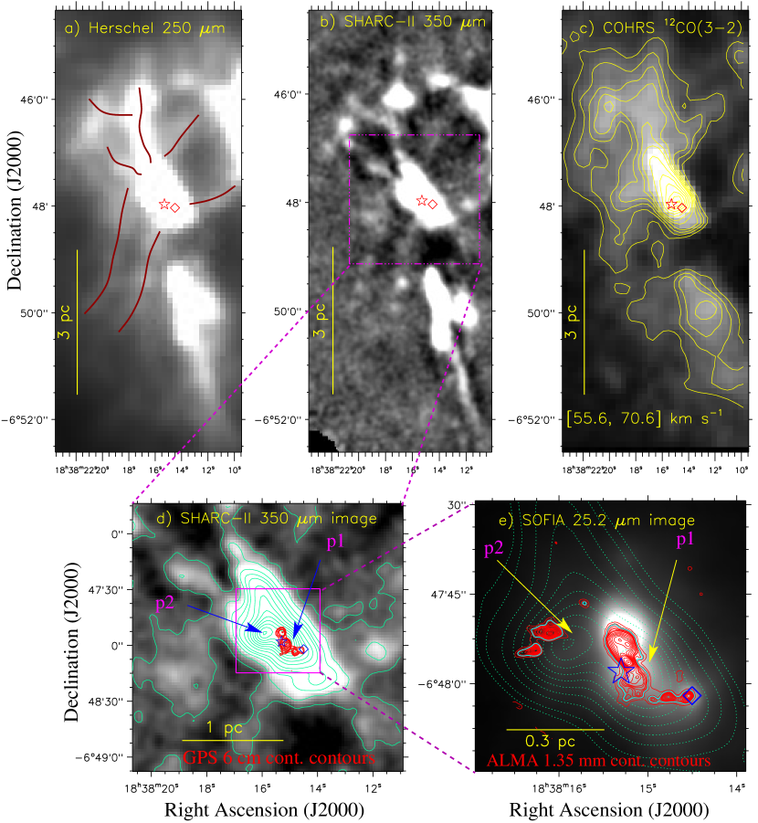
Dewangan et al. (2015b) carefully examined the Herschel sub-mm images of W42, and identified a hub-filament system in W42. Using the Herschel 250 m image, they found parsec-scale filaments, which were radially directed to the denser clump hosting the O5-O6 star and W42-MME. In Figure 14a, we present the Herschel 250 m image and highlight several filaments. Figure 14b displays the SHARC-II 350 m image, also revealing the presence of the hub-filament system in W42. In Figure 14c, we show the intensity map and contours of the COHRS 12CO(3–2) emission integrated over a velocity range of [55.6, 70.6] km s-1, displaying the central molecular condensation containing the O5-O6 star and W42-MME. The COHRS intensity map also confirms the existence of the hub-filament system in W42. Using the SHARC-II 350 m image, a zoomed-in view of the hub-filament system in W42 is presented in Figure 14d. At least two continuum peaks (i.e., p1 and p2) are evident toward the central hub in the SHARC-II 350 m image. The spatial distribution of the ionized emission traced in the GPS 6 cm continuum map is presented in Figure 14d, tracing the four ionized clumps (i.e., I1–I4) toward the SHARC-II continuum peak “p1”. Figure 14e shows a zoomed-in view of the central hub using the SOFIA 25.2 m image overlaid with the contours of the ALMA band-6 continuum emission at 1.35 mm and the SHARC-II 350 m continuum emission. The ALMA 1.35 mm continuum emission is the same as presented in Figure 2a. In Section 3.1.1, we already discussed the GPS 6 cm continuum map and the SOFIA mid-infrared image. The locations of the O5-O6 star and W42-MME are spatially seen toward the SHARC-II continuum peak “p1”, where the mid-infrared emission is prominently evident. Using the VLT/NACO adaptive-optics Ks-band and L′-band images, Dewangan et al. (2015b) examined the inner environment of the O5-O6 star (see Figure 2 in their paper). However, in the direction of the SHARC-II continuum peak “p2”, at least two 1.35 mm continuum peaks are found, and are not associated with any mid-infrared and radio emission. No K-band sources are also seen toward these two peaks (not shown here). Based on these results, the two 1.35 mm continuum peaks located toward the SHARC-II continuum peak “p2” may be candidates of massive prestellar cores, which deserve further investigation with the molecular line data. However, a detailed study of massive prestellar cores is beyond the scope of this present work.
Overall, on a large-scale picture of W42 (i.e., 3 pc 3 pc), several mm continuum cores, hosting massive stars, are investigated inside a central hub, which is surrounded by several parsec scale filaments. It implies that the material to form massive stars (including O5-O6 star and W42-MME) in W42 appears to be collected through the filaments. In a given massive star-forming region, the presence of a hub-filament configuration may hint the applicability of the GNIC scenario (Motte et al., 2018), which includes the flavours of the CA and GHC models. Hence, the GNIC scenario seems to be applicable in W42.
4.3.2 Formation process of the massive O-type star W42-MME
The massive O-type star W42-MME is embedded in the dust continuum clump, which appears to be grown by gaining the inflowing material that is channeled by the filaments (see Section 4.3.1 for more discussion).
In the direction of W42-MME, several continuum sources over a scale of 0.27 pc are evident in the ALMA continuum map at 865 m (resolution 0.′′3); six of these are MM1a, MM1b, MM2, MM3, MM4, and MM5. Over a scale of 0.1 pc, three sources, MM1a, MM1b, and MM2, are seen inside a common contour level of the ALMA continuum emission at 865 m. In the direction of the continuum source MM1a, a dusty envelope (extent 9000 AU) containing at least five continuum sources/peaks (“A–E”) is seen in the ALMA continuum map at 865 m. The continuum source “A” associated with W42-MME is found almost at the center of the dusty envelope, and is surrounded by other continuum peaks (“B–E”). Hence, the mass reservoir available for the birth of a single O-type star associated with the continuum source “A” seems plentiful. Here one can keep in mind that the continuum source MM1a (mass 2–3.8 M⊙; see Table 2) is not massive enough to form a massive star, but it hosts W42-MME and is associated with a hot molecular core. In this relation, we can suggest that cores forming massive stars do not accumulate all the mass before core collapse, but instead, cores and embedded protostars gain mass simultaneously (e.g., Zhang et al., 2009; Wang et al., 2011, 2014; Sanhueza et al., 2019; Svoboda et al., 2019). It is consistent with the GNIC scenario and/or the CA and the GHC scenarios (see Section 4.3.1).
In the maps of the H13CO+ and HCO+ emission, within a scale of 10000 AU, narrow molecular structures surrounding the continuum source “A” are evident toward the dusty envelope. The positions of the continuum sources (i.e., B, C, and D) are spatially found toward these narrow structures of the H13CO+ emission. SiO outflow lobes are spatially concentrated toward “A”, while shocks are also seen toward B and C in the SiO(8–7) emission (see Figure 8c). Mass estimation of these sources will not be accurate because they are influenced by shocks. The dusty envelope or outflow cavity (extent 9000 AU) is associated with shocks as traced in the SiO(8–7) emission. Dynamical mass of the core “A” is estimated to be 9 M⊙. The analysis of the H13CO+ profile shows the domination of the non-thermal pressure and supersonic non-thermal motions around the continuum source “A” (see Section 3.3.2).
In recent years, high resolution observations (1000s AU scale) of accreting MYSOs indicate that massive stars can form through infall from a surrounding envelope. Furthermore, the growth of an accretion disk facilitates an accretion flow onto the central object (see latest review article by Rosen et al., 2020, for more details).
Our observational outcomes also favour the onset of the disk-mediated accretion process in the MYSO W42-MME. We also propose that the core “A” accretes material from the envelope as well as from the immediate surrounding cores.
5. Summary and Conclusions
We observed in the sub-mm, mm, and cm regimes the dust, ionized emission, and molecular gas
surrounding the MYSO W42-MME (mass = 194 M⊙; luminosity 4.5 104 L⊙) using the ALMA, SMA, and VLA interferometric facilities (resolution 0.′′3–3.′′5).
Our conclusions are as follows.
An elongated filament-like feature (extent 0.15 pc) is investigated in the ALMA 1.35 mm continuum map, and is characterized as a thermally supercritical
filament. Three continuum cores (mass range 1–4.4 M⊙) are seen toward this feature,
and one of these cores (i.e., MM1; mass4.4 M⊙) hosts the MYSO W42-MME.
The ALMA 865 m continuum map reveals at least five continuum sources/peaks (“A–E”) within a dusty envelope (extent 9000 AU) toward MM1, where shocks are traced in the SiO(8–7) emission.
The continuum source “A” associated with W42-MME is found almost at the center of the dusty envelope, and is surrounded by other continuum peaks (“B–E”).
The kinetic temperature map derived using the ALMA CH3CCH lines shows the presence of a temperature gradient toward the continuum source “A”. The gas temperature ranges from 38 to 85 K.
The SMA and ALMA facilities have detected dense/hot gas tracers (13CS(5–4), HC3N(24–23), CH3CCH, CH3CN, CH3OH(51,4–42,2), and CH3OH(41,3–30,3)) and shock tracer SiO toward W42-MME.
Based on the rotational diagram analysis of several transitions of the ALMA band-6 CH3CN emission,
the rotational temperature is estimated to be 220 K. Our analysis confirms the presence of a hot molecular core associated
with W42-MME.
A molecular outflow is traced in the SMA CO(2–1) line data, and is centered at the continuum peak MM1.
The ALMA CO(3–2) line observations resolve the bipolar northeast-southwest outflow associated with the
continuum source “A”, which is distributed within a scale of 10000 AU. The bipolar outflow is also traced in the ALMA SiO(8–7), which is spatially concentrated toward
the continuum source “A”.
The molecular multiline data trace the dense cavity walls toward the dusty envelope
around W42-MME at below 10000 AU, where shocks are traced in the SiO(8–7) emission.
The continuum source MM3 has a bow-like appearance, and is associated with the H2, H2O maser, and SiO(8–7) emission.
Very strong intensities of the HCO+(4–3) and H13CO+(4–3) emission are observed toward MM3, which is located in the northern side of the dusty envelope. It seems that MM3 possibly originated from a previous ejection event from the MYSO W42-MME.
In other words, there is a signature of episodic ejections from W42-MME, favouring a disk-mediated variable accretion event.
Based on the velocity gradient seen in the ALMA multiline data (e.g., HCO+(4–3), SO, CH3OH, and NS emission), the dynamical central mass of the core hosting W42-MME is computed to be 9 M⊙. No disk inclination is considered in the calculation.
Within a scale of 2000 AU, the flattened/elongated feature is investigated in the continuum source “A” using the H13CO+(4–3) emission, and is perpendicular to the orientation of the ALMA CO outflow. A noticeable velocity gradient is also observed across the flattened/elongated feature in the CH3OH, H13CO+, SO, and NS maps.
In the direction of the continuum source “A”, the position-velocity maps of the SO, CH3OH, HCO+(4–3), and NS emission
hint the existence of a Keplerian-like rotation within a rotationally-supported disk (mass 1 M⊙). The resolution of the data is not enough for a firm conclusion.
An asymmetric self-absorbed line profile of an optically thick HCO+ line supports the signatures of infall toward the continuum source “A”. The position-velocity map of the SO emission reveals the presence of a wider “waist” like feature, which shows the signature of infalling motions in the source “A”.
Overall, our observational findings show the disk-mediated accretion process in the MYSO W42-MME.
We also suggest that the core hosting W42-MME appears to gain mass from the envelope and also from the immediate surrounding cores.
. In each panel, the positions of a 6.7 GHz MME (diamond symbol) and an O5–O6 star (star symbol) are marked.
| Name | Total Flux | FWHMx FWHMy | Mass (M⊙) | Mass (M⊙) | ||
|---|---|---|---|---|---|---|
| (h m s) | ( ′ ′′) | (mJy) | (′′ ′′) | at = 40 K | at = 70 K | |
| MM1a | 18:38:14.54 | 06:48:02.0 | 120.1 | 0.63 0.99 | 3.8 | 2.0 |
| MM1b | 18:38:14.64 | 06:48:02.9 | 14.9 | 0.69 0.61 | 0.5 | 0.2 |
| MM2 | 18:38:14.76 | 06:48:02.1 | 80.7 | 0.86 0.67 | 2.5 | 1.3 |
| MM3 | 18:38:14.67 | 06:47:57.8 | 42.9 | 0.68 1.52 | 1.3 | 0.7 |
| MM4 | 18:38:14.96 | 06:48:02.6 | 14.6 | 0.83 0.39 | 0.5 | 0.2 |
| MM5 | 18:38:14.16 | 06:48:03.5 | 29.2 | 1.21 1.40 | 0.9 | 0.5 |
References
- Anderson et al. (2009) Anderson, L. D., Bania, T. M., Jackson, J. M., et al. 2009, ApJS, 181, 255
- André et al. (2010) André, P., Men’shchikov, A., Bontemps, S., et al. 2010, A&A, 518, L102
- André et al. (2014) André, P., Di Francesco, J., Ward-Thompson, D., et al. 2014, in Protostars and Planets VI, ed. H. Beuther et al. (Tucson, AZ; Univ. Arizona Press), 27
- Andron et al. (2018) Andron, I., Gratier, P., Majumdar, L., et al. 2018, MNRAS, 481, 5651
- Araya et al. (2005) Araya, E., Hofner, P., Kurtz, S., Bronfman, L., & DeDeo, S. 2005, ApJS, 157, 279
- Arce et al. (2007) Arce, H. G., Shepherd, D., Gueth, F., et al. 2007, in Protostars and Planets V, ed. B. Reipurth, D. Jewitt, & K. Keil (Tucson, AZ: Univ. Arizona Press), 245
- Beltrán & de Wit (2016) Beltrán, M. T., & de Wit, W. J. 2016, A&ARv, 24, 6
- Benjamin et al. (2003) Benjamin, R. A.,Churchwell, E., Babler, B. L., et al. 2003, PASP, 115, 953
- Bertout (1989) Bertout, C. 1989, ARA&A, 27, 351
- Beuther et al. (2009) Beuther, H., Walsh, A. J., Longmore, S. N. 2009, ApJS, 184, 366
- Beuther et al. (2013) Beuther, H., Linz, H., Henning, Th. 2013, A&A ,558, 81
- Blum et al. (2000) Blum, R. D., Conti, P. S., & Damineli, A. 2000, AJ, 119 1860
- Bonnell et al. (2002) Bonnell, I. A., Bate, M. R., Clarke, C. J., & Pringle, J. E. 2002, MNRAS, 323, 785
- Bonnell et al. (2004) Bonnell, I. A., Vine, S. G., & Bate, M. R. 2004, MNRAS, 349, 735
- Bonnell & Bate (2006) Bonnell, I. A., & Bate, M. R. 2006, MNRAS, 370, 488
- Cesaroni et al. (2007) Cesaroni, R., Galli, D., Lodato, G., et al. 2007, Protostars and Planets V, 197
- Chen et al. (2020) Chen, Xi, Sobolev, A. M., & Breen, S. L. 2020, ApJ, 890, 22
- Dempsey, Thomas & Currie (2013) Dempsey, J. T., Thomas, H. S., & Currie, M. J. 2013, ApJS, 209, 8
- Dewangan et al. (2015a) Dewangan, L. K. , Mayya, Y. D., Luna, A., & Ojha, D. K., ApJ 2015a, 803, 100
- Dewangan et al. (2015b) Dewangan, L. K., Luna, A., Ojha, D. K., Anandarao, B. G., Mallick, K. K., Mayya, Y. D. 2015b, ApJ, 811, 79
- Dewangan (2021) Dewangan, L. K. 2021, MNRAS, 504, 1152
- Hennebelle et al. (2011) Hennebelle, P., Commerçon, B., Joos, M., et al. 2011, A&A, 528, 72
- Hennebelle & Commerçon (2014) Hennebelle, P., & Commerçon, B. 2014, ASSP, 36, 365
- Herter et al. (2012) Herter, T. L., Adams, J. D., De Buizer, J. M., et al. 2012, ApJ, 749, L18
- Hildebrand (1983) Hildebrand, R. H. 1983, Quarterly Journal of the RAS, 24, 267
- Hirota et al. (2018) Hirota, T. 2018, Publication of Korean Astronomical Society, 33, 21.
- Hoare et al. (2012) Hoare, M. G., Purcell, C. R., Churchwell, E. B., et al. 2012, PASP, 124, 939
- Hosokawa et al. (2010) Hosokawa, T., Yorke, H. W., & Omukai, K. 2010, ApJ, 721, 478
- Hunter et al. (2018) Hunter, T. R., Brogan, C. L., & MacLeod, G. C. 2018, ApJ, 854, 170
- Ilee et al. (2016) Ilee, J. D., Cyganowski, C. J., Nazari, P., et al. 2016, MNRAS, 462, 4386
- Inutsuka & Miyama (1997) Inutsuka, S. & Miyama, S. M. 1997, ApJ, 480, 681
- Jackson et al. (2006) Jackson, J. M., Rathborne, J. M., Shah, R. Y., et al. 2006, ApJS, 163, 145
- Johnston et al. (2015) Johnston, K. G., Robitaille, T. P., Beuther, H., et al. 2015, ApJ, 813, L19
- Jones et al. (2004) Jones, T. J., Woodward, C. E., & Kelley, M. S. 2004, ApJ, 128, 2448
- Kainulainen et al. (2016) Kainulainen, J., Hacar, A., Alves, J., et al. 2016 A&A 586 27
- Krumholz et al. (2009) Krumholz, M. R., Klein, R. I., McKee, C. F., et al., 2009, Science, 323, 754.
- Krumholz (2012) Krumholz, M. R. 2012, in Astronomical Society of the Pacific Conference Series, Vol. 464, Circumstellar Dynamics at High Resolution, ed. A. C. Carciofi & T. Rivinius, 339
- Kuiper et al. (2010) Kuiper, R., Klahr, H., Beuther, H., & Henning, T. 2010, ApJ , 722, 1556
- Kuiper et al. (2013) Kuiper, R. & Yorke, H. W. 2013, ApJ , 763, 104
- Kumar et al. (2020) Kumar, M. S. N., Palmeirim, P., Arzoumanian, D., & Inutsuka, S. I. 2020, A&A, 642, 87
- Lada et al. (2003) Lada, C. J., Bergin, E. A., Alves, J. F., & Huard, T. L. 2003, ApJ, 586, 286
- Lester et al. (1985) Lester, D. F., Dinerstein, H. L., Werner, M. W. et al. 1985, AJ, 296, 565
- Liu et al. (2020) Liu, S.-Y., Su, Y.-N., Zinchenko, I. I., Wang K.-S., Meyer, D. M.-A, Wang, Y., & Hsieh, I.-Ta 2020, ApJ, 904, 181
- MacLeod et al. (2018) MacLeod, G. C., Smits, D. P., & Goedhart, S. 2018, MNRAS, 478, 1077
- Malafeev et al. (2005) Malafeev, S. Yu., Zinchenko, I. I., Pirogov, L. E., & Johansson, L. E. B. 2005, AstL, 31, 239
- Marsh et al. (2015) Marsh, K. A., Whitworth, A. P., & Lomax, O. 2015, MNRAS, 454, 4282
- Marsh et al. (2017) Marsh, K. A., Whitworth, A. P., Lomax, O., et al. 2017, MNRAS, 471, 2730
- Matsakis et al. (1976) Matsakis, D. N., Evans, N. J., II, Sato, T., & Zuckerman, B. 1976, AJ, 81, 172
- Maud et al. (2018) Maud, L. T., Cesaroni, R., Kumar, M. S. N., et al. 2018, A&A, 620, A31
- Maud et al. (2019) Maud, L. T., Cesaroni, R., Kumar, M. S. N., et al. 2019, A&A, 627, L6
- McKee & Ostriker (2003) McKee, C. F. & Tan, J. C. 2003, ApJ, 585, 850
- McKee & Ostriker (2007) McKee, C. F., & Ostriker, E. C. 2007, ARAA, 45, 565
- Merello et al. (2015) Merello, M., Evans, II N. J., Shirley, Y. L., et al. 2015, ApJS, 218, 1
- Monin et al. (2007) Monin, J.-L., Clarke, C. J., Prato, L., & McCabe, C. 2007, in Protostars and Planets V, ed. B. Reipurth, D. Jewitt, & K. Keil (Tucson, AZ: Univ. Arizona Press), 395
- Molinari et al. (2010a) Molinari, S., Swinyard, B., & Bally, J. 2010a, A&A, 518, L100
- Molinari et al. (2010b) Molinari, S., Swinyard, B., Bally, J., et al. 2010b, PASP, 122, 314
- Motte et al. (2018) Motte, F., Bontemps, S., & Louvet, F. 2018, ARA&A, 56, 41
- Ossenkopf & Henning (1994) Ossenkopf, V., & Henning, T. 1994, A&A, 291, 943
- Ostriker (1964) Ostriker, J. 1964, ApJ, 140, 1056
- Padoan et al. (2020) Padoan, P., Pan, L., Juvela, M., Haugbolle, T., & Nordlund, A. 2020, ApJ, 900, 82
- Panagia (1973) Panagia, N. 1973, AJ, 78, 929
- Peters et al. (2010a) Peters, T., Banerjee, R., Klessen, R. S., et al. 2010a, ApJ, 711, 1017
- Peters et al. (2010b) Peters, T., Mac Low, M.-M., Banerjee, R., et al. 2010b, ApJ, 719, 831
- Quireza et al. (2006) Quireza, C, Rood, R. T., Balser, D. S., & Bania, T. M. 2006, ApJS, 165, 338
- Rosen et al. (2020) Rosen, A. L., Offner, S. S. R., Sadavoy, S. I., et al 2020, SSRv, 216, 62
- Sanhueza et al. (2019) Sanhueza, P., et al. ApJ, 2019, 886, 102
- Schuller et al. (2009) Schuller, F., Menten, K. M., Contreras, Y., et al. 2009, A&A, 504, 415
- Smith & Rosen (2005) Smith, M. D., & Rosen, A. 2005, MNRAS, 357, 579
- Smith et al. (2009) Smith, R. J., Longmore, S., & Bonnell, I. 2009, MNRAS, 400, 1775
- Stecklum et al. (2021) Stecklum, B., Wolf, V., Linz, H., et al. 2021, A&A, 646, 161
- Svoboda et al. (2019) Svoboda, B. E. et al. 2019, ApJ, 886, 36
- Szymczak et al. (2012) Szymczak, M., Wolak, P., Bartkiewicz, A., & Borkowski, K. M. 2012, AN, 333, 634
- Tan et al. (2014) Tan, J. C., Beltrán, M. T., Caselli, P., et al. 2014, in Protostars and Planets VI, ed. H. Beuther et al. (Tucson, AZ: Univ. Arizona Press), 149
- Tigé et al. (2017) Tigé, J., Motte, F., Russeil, D., et al. 2017, A&A, 602, A77
- Umemoto et al. (2017) Umemoto, T., Minamidani, T., Kuno, N., et al. 2017, PASJ, 69, 78
- Vázquez-Semadeni et al. (2009) Vázquez-Semadeni, E, Gómez, G. C., Jappsen, A. K., Ballesteros-Paredes, J., & Klessen, R. S. 2009, ApJ, 707, 1023
- Vázquez-Semadeni et al. (2017) Vázquez-Semadeni, E, González-Samaniego, A, & Colín, P. 2017, MNRAS, 467, 1313
- Vázquez-Semadeni et al. (2019) Vázquez-Semadeni, E., Palau, A., Ballesteros-Paredes, J., Gómez, G. C., & Zamora-Avilés, M. 2019, MNRAS, 490, 3061
- Walsh et al. (2014) Walsh, A. J., Purcell, C. R., Longmore, S. N., et al. 2014, MNRAS, 442, 2240
- Wang et al. (2011) Wang, K., Zhang, Q., Wu, Y., & Zhang, H. 2011, ApJ, 735, 64
- Wang et al. (2014) Wang, K., Zhang, Q., Testi, L., et al. 2014, MNRAS, 439, 3275
- Williams et al. (1994) Williams, J P., de Geus, E. J., & Blitz, L. 1994, ApJ, 428, 693
- Williams et al. (2012) Williams, P. K. G., Law, C. J., & Bower, G. C. 2012, PASP, 124, 624
- Woodward et al. (1985) Woodward, C. E., Helfer, H. L., & Pipher, J. L. 1985, A&A, 147, 84
- Zapata et al. (2019) Zapata, L. A., Garay, G., Palau, A., et al. 2019, ApJ, 872, 176
- Zhang et al. (2009) Zhang, Q., Wang, Y., Pillai, T., & Rathborne, J. 2009, ApJ, 696, 268
- Zhang & Tan (2011) Zhang, Y., & Tan, J. C. 2011, ApJ, 733, 55
- Zinchenko et al. (2020) Zinchenko, I. I., Liu, S.-Y., Su, Y.-N., Wang K.-S., & Wang, Y., 2020, ApJ, 889, 43
- Zinchenko et al. (2015) Zinchenko, I., Liu, S.-Y., Su, Y.-N., et al. 2015, ApJ, 810, 10
- Zinnecker & Yorke (2007) Zinnecker, H., & Yorke, H. W. 2007, ARA&A, 45, 481