Crossover polarons in a strongly interacting Fermi superfluid

Abstract

We investigate the zero-temperature quasiparticle properties of a mobile impurity immersed in a strongly interacting Fermi superfluid at the crossover from a Bose-Einstein condensate (BEC) to a Bardeen–Cooper–Schrieffer (BCS) superfluid, by using a many-body $T$-matrix approach that excludes Efimov trimer bound states. Termed BEC-BCS crossover polaron, or crossover polaron in short, this quasiparticle couples to elementary excitations of a many-body background and therefore could provide a useful probe of the underlying strongly interacting Fermi superfluid. Due to the existence of a significant pairing gap $\Delta$, we find that the repulsive polaron branch becomes less well-defined. In contrast, the attractive polaron branch is protected by the pairing gap and becomes more robust at finite momentum. It remains as a delta-function peak in the impurity spectral function below a threshold $2\Delta$. Above the threshold, the attractive polaron enters the particle-hole continuum and starts to get damped. We predict the polaron energy, residue and effective mass for realistic Bose-Fermi mixtures, where the minority bosonic atoms play the role of impurity. These results are practically useful for future cold-atom experiments on crossover polarons.

I Introduction

Polaron physics - quasiparticles formed by coupling a mobile impurity to elementary excitations of a many-particle background - has received increasing attention in the field of ultracold atoms over the last fifteen years (Massignan2014, ; Lan2014, ; Schmidt2018, ). Owing to the unprecedented controllability of interparticle interaction using Feshbach resonances (Bloch2008, ; Chin2010, ), Fermi or Bose polaron, namely, an impurity immersed in a non-interacting Fermi gas or a weakly interacting Bose gas, has now been systematically explored in the field of the cold-atom physics, both experimentally (Schirotzek2009, ; Zhang2012, ; Kohstall2012, ; Koschorreck2012, ; Cetina2016, ; Hu2016, ; Jorgensen2016, ; Scazza2017, ; Zan2019, ; Zan2020, ; Ness2020, ) and theoretically (Chevy2006, ; Lobo2006, ; Combescot2007, ; Prokofev2008, ; Massignan2008, ; Combescot2008, ; Punk2009, ; Cui2010, ; Massignan2011, ; Mathy2011, ; Schmidt2012, ; Parish2013, ; Vlietinck2013, ; Rath2013, ; Doggen2013, ; Li2014, ; Kroiss2015, ; Levinsen2015, ; Hu2016PRA, ; Goulko2016, ; Hu2018, ; Tajima2018, ; Tajima2019, ; PenaArdila2019, ; Mulkerin2019, ; Liu2019, ; Wang2019, ; Parish2021, ; Isaule2021, ; Pessoa2021, ). A unique advantage of both Fermi and Bose polarons is their simplicity. As the many-particle background is barely affected by the existence of a single impurity, we may concentrate on the impurity only. As a result, it is possible to make a quantitative comparison between experimental data and theoretical predictions (Massignan2014, ; Schmidt2018, ; Schirotzek2009, ; Scazza2017, ; Hu2018, ; Tajima2019, ; Parish2021, ; Isaule2021, ), enabling us to examine in a stringent way different approximate quantum many-particle theories (Chevy2006, ; Combescot2007, ; Combescot2008, ; Liu2019, ).

Another advantage of polarons is that they may provide a sensitive probe of the background many-particle systems. In this respect, Fermi or Bose polaron is not so useful, as the background non-interacting Fermi gas or weakly interacting Bose gas is well understood. It would be interesting to consider the polaron physics with a strongly correlated background, such as a two-component Fermi superfluid near a Feshbach resonance, which undergoes the crossover from a Bose-Einstein condensate (BEC) to a Bardeen–Cooper–Schrieffer (BCS) superfluid (Leggett1980, ; NSR1985, ; Hu2006, ). We dub the resulting quasiparticles as crossover polarons for convenience. The experimental setup can be easily achieved by utilizing a superfluid Bose-Fermi mixture, where the concentration of bosonic atoms can be reduced to reach the polaron limit. Indeed, motivated by the recent experimental demonstration of dual ⁶Li-⁷Li (FerrierBarbut2014, ), ⁶Li-⁴¹K (Yao2016, ), and ⁶Li-¹⁷⁴Yb superfluid mixtures (Roy2017, ), a moving impurity immersed in a Fermi superfluid has been considered by Nishida (Nishida2015, ) and Yi and Cui (Yi2015, ) using a Chevy’s variational ansatz, and more recently by Pierce, Leyronas and Chevy (Pierce2019, ) based on the second-order perturbation theory. In these pioneering works, the role of three-body Efimov physics has been highlighted and the unknown three-body parameter is typically introduced through a large momentum cut-off (Nishida2015, ; Yi2015, ).

The modification of the polaron spectrum due to Efimov states is definitely of great interest. However, realistically it is not clear whether the trimer states can be tuned to be resonant with the polaron state and whether these two kinds of states can have similar time-scale in dynamics so both of them can be observed simultaneously. In Bose polarons, the influence of Efimov states on the polaron physics seems to be negligible for the typical gas parameter of the background BEC (i.e., $na_{B}^{3}\sim 10^{-5})$ (Hu2016, ; Isaule2021, ). It only shows up for a highly compressible BEC when the gas parameter becomes sufficiently small (Jorgensen2016, ; Isaule2021, ). As a Fermi superfluid is less compressible than a typical BEC, naively one anticipates that the interplay between Efimov and polaron physics might be difficult to observe experimentally. In addition, the existence of Efimov trimers in some realistic experiments might be unfavored: the impurity might have a much larger mass or only strongly interact with one component of the superfluid fermions. In order to understand the polaron physics with a Fermi superfluid background in realistic experiments, it would be useful to focus on the two-body sector and separate out the effects of Efimov trimers.

The purpose of this work is to develop a theoretical framework for the two-body sector of crossover polarons, based on a non-self-consistent many-body $T$-matrix theory (Combescot2007, ). The use of the $T$-matrix approach has two obvious advantages. On the one hand, if we consider the BCS mean-field theory for the background Fermi superfluid, the $T$-matrix approach has the same accuracy of Chevy’s variational ansatz adopted earlier (Nishida2015, ; Yi2015, ), but enables us to concentrate on the two-body sector. On the other hand, it allows to go beyond the qualitative BCS description of the strongly interacting Fermi superfluid and therefore can predict quasiparticle properties of crossover polarons in a quantitative manner.

In saying that, it is worth noting that a quantitative description of the background many-body system of a strongly interacting Fermi superfluid itself is a notoriously difficult problem (Hu2006, ). Therefore, in this work, as a first attempt we would rather consider the BCS description for the Fermi superfluid (Leggett1980, ) and focus on the non-trivial role played by the pairing gap on the crossover polaron. We find that the repulsive polaron branch is less favored by a significant pairing gap $\Delta$. For the attractive polaron branch, the ground-state polaron energy at zero momentum increases due to the existence of a threshold $2\Delta$ for dressing the impurity with particle-hole excitations. However, the same threshold protects the attractive polaron and makes it long-lived at larger momentum. We predict the polaron properties for three Bose-Fermi mixtures in the polaron limit, which might be readily examined in current cold-atom laboratories.

II Many-body T-matrix approach

We consider an impurity of mass $m_{I}$ moving in a bath of spin-1/2 Fermi superfluid of equal mass $m_{\uparrow}=m_{\downarrow}=m$, described by the Hamiltonian $\mathcal{H}=\mathcal{H}_{I}+\mathcal{H}_{\textrm{int}}+\mathcal{H}_{\textrm{sf}}$. Here, $\mathcal{H}_{I}$ and $\mathcal{H}_{\textrm{sf}}$ are the Hamiltonian of the impurity and of the background Fermi superfluid, respectively, and $\mathcal{H}_{\textrm{int}}$ describes the interaction between the impurity and Fermi atoms. In the absence of the impurity-atom interaction, the impurity has an energy spectrum of free particle, i.e., $\epsilon_{\mathbf{p}}^{(I)}=\hbar^{2}\mathbf{p}^{2}/(2m_{I})$ at the momentum $\mathbf{p}$. In general, the model Hamiltonian of a strongly interacting Fermi superfluid $\mathcal{H}_{\textrm{sf}}$ is difficult to solve. From now on, let us assume that it can be exactly solved by the single-particle Green function $\mathcal{G}_{ij}(\mathcal{K}\equiv(\mathbf{k},i\omega_{m}))$ at the momentum $\mathbf{k}$ and fermionic Matsubara frequency $i\omega_{m}=(2m+1)\pi k_{B}T$, which takes the form of a 2 by 2 matrix (i.e., $i,j=1,2=\uparrow,\downarrow$) in accord with the use of the Nambu spinor $\Psi_{\mathbf{k}}=(\psi_{\mathbf{k}\uparrow},\psi_{-\mathbf{k}\downarrow}^{\dagger})^{T}$ for the atomic field operators in the broken-symmetry superfluid state. The impurity-atom interaction can be conveniently described using a contact potential (the system volume $V=1$),

$$\mathcal{H}_{\textrm{int}}=\sum_{\sigma=\uparrow,\downarrow}g_{\sigma}\sum_{\mathbf{q},\mathbf{k},\mathbf{k}^{\prime}}\psi_{\mathbf{k}\sigma}^{\dagger}c_{\mathbf{q}-\mathbf{k}}^{\dagger}c_{\mathbf{q}-\mathbf{k}^{\prime}}\psi_{\mathbf{k}^{\prime}\sigma},$$ (1)

where $c_{\mathbf{k}}$ and $c_{\mathbf{k}}^{\dagger}$ are respectively annihilation and creation field operators for the impurity, and the bare interaction strength $g_{\sigma}$ should be regularized by using the $s$-wave scattering length $a_{\sigma}$ via the standard relation, $g_{\sigma}^{-1}=m_{r}/(2\pi\hbar^{2}a_{\sigma})-\sum_{\mathbf{p}}2m_{r}/(\hbar^{2}\mathbf{p}^{2})$, with the reduced mass $m_{r}\equiv mm_{I}/(m+m_{I})$.

In the non-self-consistent $T$-matrix approach for polarons (Combescot2007, ), we keep the ladder diagram for the successive particle-particle scattering between the impurity and background fermionic atoms. However, the use of the Nambu spinor mixes the particle-hole channel for atoms (Hu2006, ). For example, the hole propagator of the spin-down atoms actually represents the propagation of particle-like excitations. This technical difficulty can be cured by taking the Green function $-\mathcal{G}_{22}(-\mathcal{K})\equiv\mathcal{G}_{11}(\mathcal{K})$ as the particle-propagator for spin-down atoms. With this consideration, we may directly write down the two-particle vertex functions $\Gamma_{ij}$ at the momentum $\mathbf{q}$ and Matsubara frequency $i\nu_{n}$ (collectively denoted as $\mathcal{Q}\equiv(\mathbf{q},i\nu_{n})$),

$$\Gamma\left(\mathcal{Q}\right)=\left[\begin{array}[]{cc}\chi_{11}\left(\mathcal{Q}\right)&\chi_{12}\left(\mathcal{Q}\right)\\ \chi_{12}\left(\mathcal{Q}\right)&\chi_{22}\left(\mathcal{Q}\right)\end{array}\right]^{-1},$$ (2)

where the two-particle propagators $\chi_{ij}(\mathcal{Q})$ are given by,

$$\chi_{11}\left(\mathcal{Q}\right) = \frac{1}{g_{\uparrow}}+\sum_{\mathcal{K}}\mathcal{G}_{11}\left(\mathcal{K}\right)G_{0}\left(\mathcal{Q}-\mathcal{K}\right),$$ (3)

$$\chi_{12}\left(\mathcal{Q}\right) = \sum_{\mathcal{K}}\mathcal{G}_{12}\left(\mathcal{K}\right)G_{0}\left(\mathcal{Q}-\mathcal{K}\right),$$ (4)

$$\chi_{22}\left(\mathcal{Q}\right) = \frac{1}{g_{\downarrow}}+\sum_{\mathcal{K}}\left[-\mathcal{G}_{22}\left(-\mathcal{K}\right)\right]G_{0}\left(\mathcal{Q}-\mathcal{K}\right),$$ (5)

$\sum_{\mathcal{K}}$ or $\sum_{\mathcal{Q}}$ stands for the short-hand notation $k_{B}T\sum_{i\omega_{m}}\sum_{\mathbf{k}}$ or $k_{B}T\sum_{i\nu_{n}}\sum_{\mathbf{q}}$, and $G_{0}(\mathcal{Q}-\mathcal{K})=1/[i\nu_{n}-i\omega_{m}-\epsilon_{\mathbf{q}-\mathbf{k}}^{(I)}]$ is the non-interacting Green function of the impurity. The self-energy $\Sigma(\mathcal{K})=\Sigma_{11}+2\Sigma_{12}+\Sigma_{22}$ of the impurity then takes the form (Combescot2007, ),

$$\Sigma_{11}\left(\mathcal{K}\right) = +\sum_{\mathcal{Q}}\Gamma_{11}\left(\mathcal{Q}\right)\mathcal{G}_{11}\left(\mathcal{Q}-\mathcal{K}\right),$$ (6)

$$\Sigma_{12}\left(\mathcal{K}\right) = -\sum_{\mathcal{Q}}\Gamma_{12}\left(\mathcal{Q}\right)\mathcal{G}_{12}\left(\mathcal{Q}-\mathcal{K}\right),$$ (7)

$$\Sigma_{22}\left(\mathcal{K}\right) = +\sum_{\mathcal{Q}}\Gamma_{22}\left(\mathcal{Q}\right)\left[-\mathcal{G}_{22}\left(\mathcal{-Q}+\mathcal{K}\right)\right],$$ (8)

where the different sign in $\Sigma_{11}$ (or $\Sigma_{22}$) and $\Sigma_{12}$ is due to the absence of a Fermi loop in the diagram for $\Sigma_{12}$.

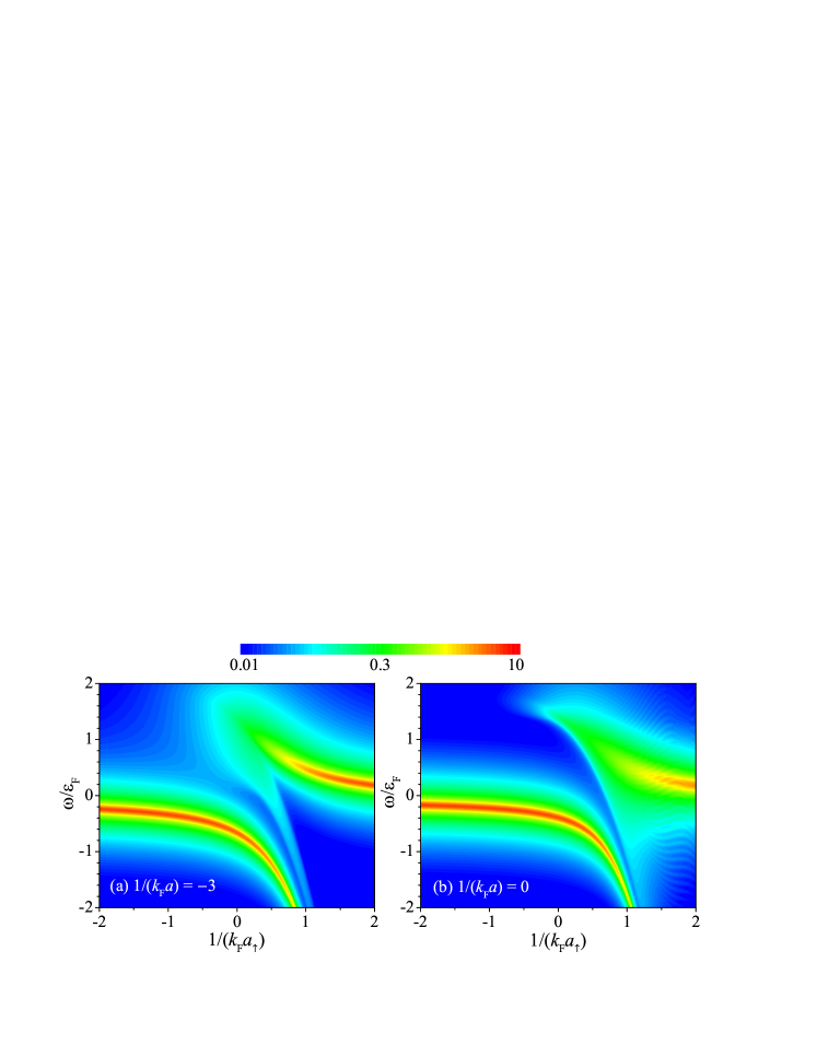
Figure 1: The evolution of the zero-momentum impurity spectral function $A(\mathbf{k}=0,\omega$) as a function of the scattering length $a_{\uparrow}$ between the impurity and spin-up atoms, with a weakly-interacting Fermi gas background (i.e., $1/(k_{F}a)=-3$ in (a)) or with a unitary Fermi superfluid background ($1/(k_{F}a)=0$ in (b)). The interaction parameter between the impurity and spin-down atoms is set to be $1/(k_{F}a_{\downarrow})=-5$. A small linewidth broadening factor $\eta=0.05\varepsilon_{F}$ has been introduced to better illustrate the $\delta$-function peak of attractive polaron branch. The spectral function is in units of $\varepsilon_{F}^{-1}$, where $\varepsilon_{F}\equiv\hbar^{2}k_{F}^{2}/(2m)$ is the Fermi energy. We always take the equal mass for the impurity and atoms, $m_{I}=m$, except the realistic experimental case in Fig. 6.

II.1 BCS Fermi superfluid

The above expressions for the two-particle vertex function and impurity self-energy are quantitatively useful, provided that the Green functions $\mathcal{G}_{ij}(\mathcal{K})$ of the background Fermi superfluid are known to a certain accuracy. Here, we are interested in understanding the general picture of the crossover polaron, with the help of the qualitatively reliable mean-field theory for Fermi superfluids. The consideration of strong pair fluctuations to $\mathcal{G}_{ij}(\mathcal{K})$ at the BEC-BCS crossover is postponed to a future study.

In the mean-field framework, the single-particle Green functions $\mathcal{G}_{ij}(\mathcal{K})$ are well-known (Leggett1980, ; Hu2006, ):

$$\mathcal{G}_{11}\left(\mathcal{K}\right) = \frac{u_{\mathbf{k}}^{2}}{i\omega_{m}-E_{\mathbf{k}}}+\frac{v_{\mathbf{k}}^{2}}{i\omega_{m}+E_{\mathbf{k}}},$$ (9)

$$\mathcal{G}_{12}\left(\mathcal{K}\right) = \frac{u_{\mathbf{k}}v_{\mathbf{k}}}{i\omega_{m}-E_{\mathbf{k}}}+\frac{u_{\mathbf{k}}v_{\mathbf{k}}}{i\omega_{m}+E_{\mathbf{k}}},$$ (10)

where $E_{\mathbf{k}}\equiv\sqrt{\xi_{\mathbf{k}}^{2}+\Delta^{2}}$ with $\xi_{\mathbf{k}}\equiv\epsilon_{\mathbf{k}}-\mu=\hbar^{2}\mathbf{k}^{2}/(2m)-\mu$ is the Bogoliubov quasiparticle energy for a Fermi superfluid with chemical potential $\mu$ and pairing gap $\Delta$, and $u_{\mathbf{k}}^{2}=[1+\xi_{\mathbf{k}}/E_{\mathbf{k}}]/2$, $v_{\mathbf{k}}^{2}=1-u_{\mathbf{k}}^{2}$, and $u_{\mathbf{k}}v_{\mathbf{k}}=\Delta/(2E_{\mathbf{k}})$ are the quasiparticle wavefunctions. Both $\mu$ and $\Delta$ can be calculated for a given dimensionless interaction parameter $1/(k_{F}a)$ (Leggett1980, ), where $a$ is the $s$-wave length between unlike atoms and $k_{F}=(3\pi^{2}n)^{1/3}$ is Fermi wavevector at the number density $n$ of the Fermi superfluid. After plugging the above $\mathcal{G}_{ij}(\mathcal{K})$ and the free impurity Green function $G_{0}(\mathcal{Q}-\mathcal{K})$ into the expressions of the two-particle propagators, we find that at zero temperature,

$$\chi_{dd}\left(\mathcal{Q}\right) = -\sum_{\mathbf{p}}\left[\frac{u_{\mathbf{p}}^{2}}{i\nu_{n}-E_{\mathbf{p}}-\epsilon_{\mathbf{q}-\mathbf{p}}^{(I)}}+\frac{2m_{r}}{\hbar^{2}\mathbf{p}^{2}}\right],$$ (11)

$$\chi_{12}\left(\mathcal{Q}\right) = -\sum_{\mathbf{p}}\frac{u_{\mathbf{p}}v_{\mathbf{p}}}{i\nu_{n}-E_{\mathbf{p}}-\epsilon_{\mathbf{q}-\mathbf{p}}^{(I)}},$$ (12)

and $\chi_{11}(\mathcal{Q})=m_{r}/(2\pi\hbar^{2}a_{\uparrow})+\chi_{dd}(\mathcal{Q})$ and $\chi_{22}(\mathcal{Q})=m_{r}/(2\pi\hbar^{2}a_{\downarrow})+\chi_{dd}(\mathcal{Q})$. Using the fact that there is no macroscopic population of the impurity state, we can analytically perform the Matsubara frequency summation in the expressions of $\Sigma_{ij}(\mathcal{K})$ (Combescot2007, ). Thus, after analytic continuation ($i\omega_{m}\rightarrow\omega^{+}\equiv\omega+i0^{+}$) we obtain the zero-temperature retarded self-energies,

$$\Sigma_{11}\left(\mathbf{k},\omega\right) = +\sum_{\mathbf{q}}v_{\mathbf{q}-\mathbf{k}}^{2}\Gamma_{11}\left(\mathbf{q},\omega^{+}-E_{\mathbf{q}-\mathbf{k}}\right),$$ (13)

$$\Sigma_{12}\left(\mathbf{k},\omega\right) = -\sum_{\mathbf{q}}u_{\mathbf{q}-\mathbf{k}}v_{\mathbf{q}-\mathbf{k}}\Gamma_{12}\left(\mathbf{q},\omega^{+}-E_{\mathbf{q}-\mathbf{k}}\right),$$ (14)

$$\Sigma_{22}\left(\mathbf{k},\omega\right) = +\sum_{\mathbf{q}}v_{\mathbf{q}-\mathbf{k}}^{2}\Gamma_{22}\left(\mathbf{q},\omega^{+}-E_{\mathbf{q}-\mathbf{k}}\right).$$ (15)

The retarded interacting impurity Green function is then given by $G(\mathbf{k},\omega)=1/[\omega-\epsilon_{\mathbf{k}}^{(I)}-\Sigma(\mathbf{k},\omega)]$, and its pole position determines the polaron energy, i.e.,

$$\mathcal{E}_{P}\left(\mathbf{k}\right)=\epsilon_{\mathbf{k}}^{(I)}+\Sigma\left[\mathbf{k},\mathcal{E}_{P}\left(\mathbf{k}\right)\right].$$ (16)

By expanding the self-energy near the zero momentum $\mathbf{k}=0$ and the ground-state polaron energy $\mathcal{E}_{P}\equiv\mathcal{E}_{P}\left(\mathbf{0}\right)$, we can calculate directly the polaron residue $\mathcal{Z}^{-1}=1-\partial\textrm{Re}\Sigma(0,\omega)/\partial\omega$ and the effective mass $m_{*}/m_{I}=\mathcal{Z}^{-1}/[1+\partial\textrm{Re}\Sigma(\mathbf{k},\mathcal{E}_{P})/\partial\epsilon_{\mathbf{k}}^{(I)}]$.

II.2 Link to Chevy’s ansatz

At this stage, it is beneficial to clarify the connection of our many-body $T$-matrix formalism to Chevy’s variational ansatz (Chevy2006, ; Combescot2007, ). Let us focus on the simplest case with zero interaction between the impurity and spin-down atoms ($a_{\downarrow}=0^{-}$), where $\chi_{22}\rightarrow-\infty$ so the only remaining two-particle vertex function is $\Gamma_{11}$. It is readily seen that the equation for the polaron energy Eq. (16) can be rewritten as,

$$\mathcal{E}_{P}\left(\mathbf{k}\right) = \epsilon_{\mathbf{k}}^{(I)}+\sum_{\mathbf{q}}v_{\mathbf{q}}^{2}\left[\frac{m_{r}}{2\pi\hbar^{2}a_{\uparrow}}-\sum_{\mathbf{p}}\frac{2m_{r}}{\hbar^{2}\mathbf{p}^{2}}\right.$$ (17)

$$\left.+\sum_{\mathbf{p}}\frac{u_{\mathbf{p}}^{2}}{E_{\mathbf{p}}+\epsilon_{\mathbf{k}+\mathbf{q}-\mathbf{p}}^{(I)}+E_{\mathbf{q}}-\mathcal{E}_{P}\left(\mathbf{k}\right)}\right]^{-1}.$$

In the case of an ideal Fermi gas background with a vanishing pairing gap $\Delta=0$, we have $v_{\mathbf{q}}^{2}=\Theta(k_{F}-q)$, $u_{\mathbf{p}}^{2}=\Theta(p-k_{F})$, $E_{\mathbf{p}}=\epsilon_{\mathbf{p}}-\mu$ and $E_{\mathbf{q}}=\mu-\epsilon_{\mathbf{q}}$, where $\Theta(x)$ is the Heaviside step function. Thus, we recover the celebrated equation for polaron energy from Chevy’s variational ansatz (see Eq. (2) in the seminal work (Combescot2007, )). For the alternative derivation of Eq. (17) by using Chevy’s ansatz with the standard BCS variational wave-function, we refer to Appendix A.

II.3 Remarks on the BEC limit

The above formalisms are quantitatively applicable to the BCS limit and are qualitatively applicable in the unitary or crossover regime. Towards the BEC limit, the fermionic degree of freedom, as characterized by the Green functions $\mathcal{G}_{ij}(\mathcal{K})$, is suppressed. The new bosonic degree of freedom, represented by the vertex function of the Fermi superfluid NSR1985 ; Hu2006 , become dominant. As a result, our formalisms based on the non-self-consistent $T$-matrix theory fail. We need to construct a theory beyond the ladder approximation, by considering the exact three-body interaction vertex involving a Cooper pair and the impurity that describes the dressing of the impurity with the gapless phonon excitations of the Fermi superfluid Hu2006 . In this way, we are anticipated to recover Bose polarons occurring in the weakly-interacting BEC limit Rath2013 ; PenaArdila2019 .

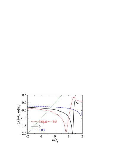
Figure 2: The zero-momentum impurity self-energy at different background Fermi superfluids characterized by the interaction parameter, $1/(k_{F}a)=-0.5$ (red dashed line), $0$ (black solid line), and $+0.5$ (blue dot-dashed line). The thin green dashed line shows the straight line $h(\omega)=\omega$. The intersection of the straight line and the self-energy curve determines the polaron energy at zero momentum. Here, we take the impurity-atom interactions: $1/(k_{F}a_{\uparrow})=0$ and $a_{\downarrow}=0^{-}$. The two times pairing gap for each curve is: $2\Delta\simeq 0.804\varepsilon_{F}$ at $1/(k_{F}a)=-0.5$, $2\Delta\simeq 1.373\varepsilon_{F}$ in the unitary limit, and $2\Delta\simeq 2.033\varepsilon_{F}$ at $1/(k_{F}a)=+0.5$.

III Results and discussions

Before we present the results, let us briefly discuss how the paired Fermi superfluid background is affected by the moving impurity. Dynamically, if we take a snapshot, an impurity will excite density fluctuations of the total density (i.e., charge degree of freedom) and of the spin density (i.e., spin degree of freedom) at the impurity site, which propagate over the whole Fermi superfluid. As the impurity moves, the fluctuations generated at different time interfere and after a timescale set by the inverse Fermi energy the fluctuations fade away. In the limit of a single impurity, therefore in equilibrium the Fermi superfluid is essentially not perturbed, since the perturbation strength scales like $1/N$, where $N$ is the total number of fermions of the background system.

The situation may dramatically change if the mass of the impurity is very large. For example, an infinitely heavy impurity will create a static scattering potential and therefore lead to a permanent local distortion of the Fermi superfluid near the impurity. For a static non-magnetic impurity scattering (i.e., $a_{\uparrow}=a_{\downarrow}$), the single-particle energy spectrum of the Fermi superfluid is essentially unchanged, according to Anderson’s theorem Anderson1959 ; Balatsky2006 . For a static magnetic impurity scattering ($a_{\uparrow}\neq a_{\downarrow}$) that lifts the Kramers degeneracy of the pairing states (or breaks the time-reversal symmetry) and excites spin-density fluctuations, a non-trivial Yu-Shiba-Rusinov (YSR) bound state appears within the energy gap $2\Delta$ Yu1965 ; Shiba1968 ; Rusinov1969 ; Vernier2011 ; Jiang2011 .

The existence of the YSR bound state in the case of a moving impurity requires a further investigation. Naïvely, we may anticipate the appearance of a sub-gap band of YSR states, whose number is proportional to the number of impurities or impurity density (which scales to zero in the single impurity limit). In our non-self-consistent $T$-matrix approach, we consider the single-impurity limit and hence neglect again the coupling of the YSR bound state to the polaron in the thermodynamic limit. Nevertheless, in the static limit the impurity properties could be profoundly affected by the YSR bound state, since we probe exactly the neighborhood of the impurity (instead of the whole system for a moving impurity).

III.1 The significance of a pairing gap

Appendix A shows that Eq. (17) can be understood as an extension of Chevy’s ansatz in the case of a Fermi superfluid background. It describes the virtual process of dressing the impurity with simultaneous particle- and hole-like excitations, each of which has the possibility $u_{\mathbf{p}}^{2}$ or $v_{\mathbf{q}}^{2}$, and energy $E_{\mathbf{p}}$ or $E_{\mathbf{q}}$. The appearance of the summation $E_{\mathbf{p}}+E_{\mathbf{q}}$ in the denominator of Eq. (17) is a direct consequence of breaking a Cooper pair during the virtual excitation. It naturally leads to a threshold $2\Delta$ for the one-particle-hole excitation, which may change the polaron spectrum in a non-trivial way.

To see this, in Fig. 1 we show the impurity spectral function $A(\mathbf{k},\omega)\equiv-\textrm{(1/$\pi$)Im}G(\mathbf{k},\omega)$ at zero momentum $\mathbf{k}=0$ as a function of the dimensionless impurity-atom interaction $1/(k_{F}a_{\uparrow})$. For a negligible pairing gap in (a), we find the typical spectrum for a Fermi polaron with both attractive branch and repulsive branch (Massignan2011, ), and a narrow molecule-hole continuum in between (Massignan2011, ; Parish2021, ). There are notable changes in the spectrum when we take a unitary Fermi gas as the background with a significant (mean-field) pairing gap $\Delta\simeq 0.69\varepsilon_{F}$. The repulsive branch becomes much blurred, indicating the shorter lifetime of repulsive polarons. At the same time, the parameter window for their existence shrinks. The molecule-hole continuum also disappears. In contrast, the attractive branch remains well-defined, but the ground-state energy of attractive polarons seems to increase systematically.

As the repulsive polaron can be naïvely viewed as the excited state of the molecule (with the dressing of particle-hole excitations), the less well-defined repulsive polaron may be understood from the fact that the molecule consisting of the impurity and spin-up atoms becomes more difficult to form due to the energy cost for Cooper pair-breaking. This idea is consistent with the disappearance of the molecule-hole continuum.

On the other hand, the upshift of the attractive polaron energy can be easily understood from the particle-hole excitation threshold $2\Delta$, which leads to a larger self-energy for the impurity, as shown in Fig. 2, where we plot the zero-momentum self-energy at various superfluid pairing gaps and at the unitary coupling between the impurity and spin-up atoms (i.e., $1/(k_{F}a_{\uparrow})=0$). By increasing the background interaction parameter $1/(k_{F}a)$ and hence the pairing gap, the impurity self-energy shifts up at the negative frequency. As a result, the polaron energy of the solution $\mathcal{E}_{P}=\Sigma(0,\mathcal{E}_{P})$, which is given by the intersection of the straight line $h(\omega)=\omega$ and the self-energy curve $\Sigma(0,\omega)$, becomes larger.

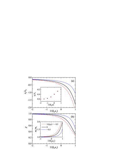
Figure 3: Polaron energy (a), residue (b) and effective mass (the inset in (b)) as a function of the dimensionless impurity-atom interaction parameter $1/(k_{F}a_{\uparrow})$ at three different background Fermi superfluids with $1/(k_{F}a)=-0.5$ (red dashed line), $0$ (black solid line), and $+0.5$ (blue dot-dashed line). The inset in (a) shows the polaron energy as a function of $1/(k_{F}a)$ at the unitary coupling $1/(k_{F}a_{\uparrow})=0$. For all the plots in the figure, we consider the non-interacting limit between the impurity and spin-down atoms (i.e., $a_{\downarrow}=0^{-}$).

III.2 Equal mass case

From now on, let us concentrate on well-defined attractive polarons, which are easier to measure in experiments (Schirotzek2009, ). In Fig. 3(a), we present the polaron energy as a function of $1/(k_{F}a_{\uparrow})$ at $a_{\downarrow}=0^{-}$ and at three different Fermi superfluid background. The increase of the polaron energy as a function of the background interaction parameter $1/(k_{F}a)$ is highlighted in the inset, where we take a unitary coupling ($a_{\uparrow}\rightarrow\pm\infty$) between the impurity and spin-up atoms. This is the most interesting case, in which we may define a universal energy parameter (Hu2006, ) for crossover polarons, i.e., $\mathcal{E}_{P}=\xi(1/k_{F}a)\varepsilon_{F}$. From the inset, we find that towards the BCS limit of Fermi superfluid the energy parameter $\xi$ quickly saturates to the well-known result for Fermi polarons, i.e., $\xi(a=0^{-})\simeq-0.607$ (Chevy2006, ; Combescot2007, ). For a unitary Fermi superfluid background, it increases to $\xi(a=\pm\infty)\simeq-0.396$. Although the difference between these two values $\Delta\xi=\xi(a=\pm\infty)-\xi(a=0^{-})\simeq 0.211$ is not significant, it is slightly larger than the experimental resolution in determining the polaron energy via the radio-frequency spectroscopy (i.e., $\sim 0.1\varepsilon_{F}$) Schirotzek2009 ; Scazza2017 ; Zan2019 and therefore might be experimentally measured. We note that, the difference $\Delta\xi$ may also quantitatively change, if we go beyond the mean-field treatment of the strongly interacting Fermi superfluid background.

In line with the decreasing absolute value of the polaron energy within a strongly interacting Fermi superfluid, the residue and effective mass of the polaron increases and decreases, respectively, as reported in Fig. 3(b). In particular, at the unitary impurity-atom coupling ($a_{\uparrow}=\pm\infty$), we obtain a residue $Z\simeq 0.90$ and an effective mass $m_{*}/m_{I}\simeq 1.07$ with a unitary Fermi superfluid, in comparison to the predictions of $Z\simeq 0.78$ and $m_{*}/m_{I}\simeq 1.17$ in the case of Fermi polarons (Combescot2007, ).

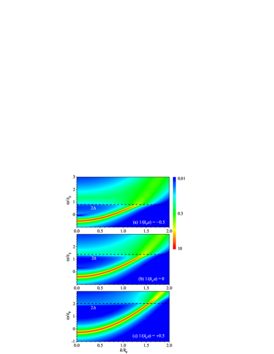
Figure 4: Two-dimensional contour plot of the impurity spectral function $A(k,\omega)$ at three different background Fermi superfluids with $1/(k_{F}a)=-0.5$ (a), $0$ (b), and $+0.5$ (c). We consider the unitary coupling between the impurity and spin-up atoms ($a_{\uparrow}=\pm\infty$) and zero coupling between the impurity and spin-down atoms ($a_{\downarrow}=0^{-}$). The black dashed lines indicate the particle-hole excitation thresholds, $2\Delta\simeq 0.804\varepsilon_{F}$ in (a) $2\Delta\simeq 1.373\varepsilon_{F}$ in (b) and $2\Delta\simeq 2.033\varepsilon_{F}$ in (c). We use a small linewidth broadening factor $\eta=0.05\varepsilon_{F}$ to better show the $\delta$-peak of attractive polaron branch. The spectral function is in units of $\varepsilon_{F}^{-1}$.

We consider so far the ground-state polaron at zero momentum. At finite momentum, in general the polaron will have a finite lifetime, once its energy reaches the minimum energy of the particle-hole continuum. For Fermi polarons, this occurs at zero energy $\omega=0$ in the absence of two-body molecular bound states (i.e., $a_{\uparrow}\leq 0$). For crossover polarons with a significant background pairing gap $\Delta\sim O(\varepsilon_{F})$, Eq. (17) indicates that we have a threshold $2\Delta$ for particle-hole excitations and therefore the crossover polaron should remain as a long-lived quasiparticle as long as its energy is smaller than $2\Delta$. This anticipation is examined in Fig. 4, where we present two-dimensional contour plots of the finite-momentum impurity spectral function $A(\mathbf{k},\omega)$ at three background Fermi superfluids. The threshold $2\Delta$ has been shown in the figures by using black dashed lines. It is readily seen that the polaron remains as a $\delta$-function peak, provided that $\mathcal{E}_{P}+\hbar^{2}k^{2}/(2m_{*})<2\Delta$. This gives rise to a characteristic momentum $k_{c}=\sqrt{2m^{*}(2\Delta-\mathcal{E}_{P})}/\hbar$, below which the polaron is long-lived. We find that $k_{c}$ increases with increasing pairing gap, suggesting the polaron becomes more robust with a strongly interacting Fermi superfluid background. Finally, if the impurity spectral function can be experimentally measured by the momentum-resolved radio-frequency spectroscopy, one may directly determine the threshold $2\Delta$. This provides a possible way to measure the pairing gap of the Fermi superfluid background.

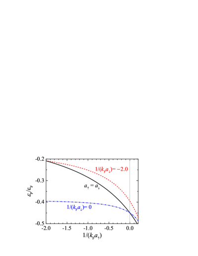
Figure 5: The effect of the interaction between the impurity and spin-down atoms on the polaron energy. Here, we consider a unitary Fermi superfluid as the background ($a=\pm\infty$) and three cases for the interaction between the impurity and spin-down atom: $1/(k_{F}a_{\downarrow})=-0.5$ (red dashed line), $1/(k_{F}a_{\uparrow})$ (black solid line), and $0$ (blue dot-dashed line).

III.3 Role of the interaction with spin-down atoms

In previous calculations, we take a negligible interaction between the impurity and spin-down atoms. This is the typical situation in experiments since it is difficult to tune the two scattering lengths $a_{\uparrow}$ and $a_{\downarrow}$ to be large simultaneously. In Fig. 5, we report the exceptional case that the impurity interacts strongly with both spins. At the unitary coupling ($a_{\uparrow}=a_{\downarrow}=\pm\infty$) with a unitary Fermi superfluid background ($a=\pm\infty$), we find the polaron energy $\mathcal{E}_{P}\simeq-0.450\varepsilon_{F}$.

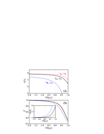
Figure 6: Polaron energy (a), residue (b) and effective mass (the inset in (b)) as a function of the dimensionless impurity-atom interaction parameter $1/(k_{F}a_{\uparrow})$ for the mixtures of ⁶Li-⁴¹K (red dashed line), ⁶Li-⁷Li (black line) and ⁴⁰K-⁷Li (blue dot-dashed line). We consider a unitary Fermi superfluid as the background ($a=\pm\infty$) and take $1/(k_{F}a_{\downarrow})=-5$ for the interaction between the impurity and spin-down atoms.

III.4 Experimental relevance

Let us finally explore the possibility of experimentally observing the predicted crossover polaron. A straightforward idea is to use the recently realized dual Bose-Fermi superfluid (FerrierBarbut2014, ; Yao2016, ; Roy2017, ). In the limit of small bosonic density, the bosons can be treated as independent impurities and their properties can be directly measured by using rf (Schirotzek2009, ) or Raman spectroscopy (Ness2020, ). Fermi-Fermi mixtures involving a (majority) two-component Fermi superfluid and another (minority) normal Fermi gas, such as a paired ⁶Li superfluid with ⁴⁰K atoms as impurities, may also be possible candidates.

In Fig. 6, we show the polaron energy, residue and effective mass in three Bose-Fermi mixtures with different mass ratio $m_{I}/m$. For a lighter impurity, quasiparticle properties appear to have a more sensitive dependence on the impurity-atom interaction.

The experimental challenge of realizing a crossover polaron lies in the difficulty of independently tuning the impurity-atom interaction $a_{\uparrow}$, in addition to the control of the scattering length $a$ for the background Fermi superfluid. This would require a significant overlap between two Feshbach resonances for enlarging $a_{\uparrow}$ and $a$, respectively. A careful search for the best candidate system, through detailed two-body calculations for various $s$-wave scattering lengths, will be addressed in future works.

IV Conclusions and outlooks

In summary, we have presented a many-body $T$-matrix theory for a novel type of crossover polaron, which can be potentially realized in dual Bose-Fermi superfluids, where the minority bosonic atoms can be treated as impurities. By using a mean-field description for the background strongly interacting Fermi superfluid, we have qualitatively clarified the role played by the pairing gap on polaron physics. We have found that the repulsive polaron branch ceases to exist. In contrast, attractive polarons become robust at finite momentum. In the near future, we will investigate quantitative corrects to the polaron quasiparticle properties due to strong pair fluctuations in the background Fermi superfluid. Another interesting possibility is to consider a topological Fermi superfluid as the background and to study how the polaron physics changes near the topological phase transition (Bai2018, ).

In our work, we do not consider the Efimov trimer bound states, which may become important under specific conditions (with fine-tuning interaction parameters). To address these trimer states and their interplay with polaron states, we need to go beyond the current non-self-consistent many-body $T$-matrix approach as discussed in Sec. IIC. A simple way is to include the non-trivial vertex correction to the vertex function $\Gamma(\mathcal{Q})$. In other words, we need to consider the contribution of particle-hole diagrams to $\Gamma(\mathcal{Q})$, together with the particle-particle ladder diagrams as given in Eqs. (3), (4) and (5). The particle-hole diagrams take into account the multiple particle-hole excitations near Fermi surfaces and capture the contribution of Efimov states Punk2009 ; Nishida2015 ; Yi2015 ; Pierce2019 . This non-trivial extension of the many-body $T$-matrix theory will be considered in future studies.

Appendix A Variational Ansatz Approach

Here we give the details on deriving the polaron energy relation, i.e., Eq. (17) in the main text, by using an extended Chevy’s ansatz approach with the standard BCS variational wave-functions for the case of a vanishing interaction $g_{\downarrow}=0$ between the impurity and spin-down fermions.

The Hamiltonian is given by $\mathcal{H}=\mathcal{H}_{I}+\mathcal{H}_{{\rm int}}+\mathcal{H}_{{\rm sf}}$. The first term is the Hamiltonian for the impurity, $\mathcal{H}_{I}=\sum_{\mathbf{k}}\epsilon_{\mathbf{k}}^{(I)}c_{\mathbf{k}}^{\dagger}c_{\mathbf{k}}$, with $\epsilon_{\mathbf{k}}^{(I)}=\hbar^{2}\mathbf{k}^{2}/(2m_{I})$. Here, $c_{\mathbf{k}}^{\dagger}$ and $c_{\mathbf{k}}$ are the annihilation and creation field operators for the impurity, respectively. The impurity-fermion interaction is given by (the system volume $V=1$)

$$\mathcal{H}_{\text{int }}=g_{\uparrow}\sum_{\mathbf{q},\mathbf{k},\mathbf{k}^{\prime}}\psi_{\mathbf{k}\uparrow}^{\dagger}c_{\mathbf{q}-\mathbf{k}}^{\dagger}c_{\mathbf{q}-\mathbf{k}^{\prime}}\psi_{\mathbf{k}^{\prime}\uparrow}$$ (18)

for the $g_{\downarrow}=0$ case, and the Hamiltonian for the two-component Fermi superfluid is given by

$$\mathcal{H}_{{\rm sf}}=\sum_{\sigma=\uparrow,\downarrow}\sum_{\mathbf{k}}\left(\epsilon_{\mathbf{k}}-\mu\right)\psi_{\mathbf{k}\sigma}^{\dagger}\psi_{\mathbf{k}\sigma}+g\sum_{\mathbf{k},\mathbf{k}^{\prime},\mathbf{q}}\psi_{\mathbf{k}\uparrow}^{\dagger}\psi_{\mathbf{q}-\mathbf{k}\downarrow}^{\dagger}\psi_{\mathbf{q}-\mathbf{k}^{\prime}\downarrow}\psi_{\mathbf{k}^{\prime}\uparrow},$$ (19)

where $\epsilon_{\mathbf{k}}=\hbar^{2}\mathbf{k}^{2}/(2m)$ is the dispersion relation for a free fermion; $\mu$ is the chemical potential; $\psi_{\sigma}^{\dagger}$ and $\psi_{\sigma}$ are the annihilation and creation field operators for the $\sigma$-component ($\sigma=\uparrow,\downarrow$) fermion, respectively. The bare interaction strength $g_{\uparrow}$ (or $g$) should be regularized by using the $s$-wave scattering length $a_{\uparrow}$ (or $a$) via the standard regularization relation. For example, $g_{\uparrow}^{-1}=m_{r}/\left(2\pi\hbar^{2}a_{\uparrow}\right)-\sum_{\mathbf{p}}2m_{r}/\left(\hbar^{2}\mathbf{p}^{2}\right)$, with the reduced mass $m_{r}\equiv mm_{I}/\left(m+m_{I}\right)$.

In a standard mean-field approach of studying the BCS-BEC crossover, the superfluid Hamiltonian can be approximated by

$$\mathcal{H}_{{\rm sf}}\approx\langle\mathcal{H}_{{\rm sf}}\rangle_{{\rm MF}}+\sum_{\sigma=\uparrow,\downarrow}\sum_{\mathbf{k}}E_{\mathbf{k}}\alpha_{\mathbf{k}\sigma}^{\dagger}\alpha_{\mathbf{k}\sigma},$$ (20)

where the mean-field ground state energy

$$\langle\mathcal{H}_{{\rm sf}}\rangle_{{\rm MF}}=-\frac{\Delta^{2}}{g}+\sum_{\mathbf{k}}(\epsilon_{\mathbf{k}}-\mu-E_{\mathbf{k}})=-\frac{m\Delta^{2}}{4\pi\hbar^{2}a}+\sum_{\mathbf{k}}(\epsilon_{\mathbf{k}}-\mu-E_{\mathbf{k}}+\frac{\Delta^{2}}{2\epsilon_{\mathbf{k}}})$$ (21)

is a constant and will be neglected hereafter. Here, $\Delta=g\sum_{\mathbf{k}}\langle\psi_{-\mathbf{k}\downarrow}\psi_{\mathbf{k}\uparrow}\rangle$ is the mean-field pairing gap. The quasi-particle excitation spectrum $E_{\mathbf{k}}=\sqrt{\xi_{\mathbf{k}}^{2}+\Delta^{2}}\equiv\sqrt{(\epsilon_{\mathbf{k}}-\mu)^{2}+\Delta^{2}}$ and the corresponding creation (annihilation) operators $\alpha_{\mathbf{k}\sigma}^{\dagger}$ ($\alpha_{\mathbf{k}\sigma}$) can be obtained by a Bogoliubov transformation

$$\left(\begin{array}[]{c}\alpha_{\mathbf{k}\uparrow}\\ \alpha_{-\mathbf{k}\downarrow}^{\dagger}\end{array}\right)=\left(\begin{array}[]{cc}u_{\mathbf{k}}&-v_{\mathbf{k}}\\ v_{\mathbf{k}}&u_{\mathbf{k}}\end{array}\right)\left(\begin{array}[]{c}\psi_{\mathbf{k}\uparrow}\\ \mathrm{\psi}_{-\mathbf{k}\downarrow}^{\dagger}\end{array}\right),$$ (22)

where $u_{\mathbf{k}}^{2}=\left[1+\xi_{\mathbf{k}}/E_{\mathbf{k}}\right]/2$, $v_{\mathbf{k}}^{2}=1-u_{\mathbf{k}}^{2}$, and $u_{\mathbf{k}}v_{\mathbf{k}}=\Delta/\left(2E_{\mathbf{k}}\right)$ are the quasiparticle wavefunctions. With the quasiparticle operators, the impurity-fermion interaction can be written as,

$$\begin{aligned} \mathcal{H}_{{\rm int}}&=g_{\uparrow}\sum_{\mathbf{k},\mathbf{k}^{\prime},\mathbf{q}}\left(u_{\mathbf{k}}\alpha_{\mathbf{k}\uparrow}^{\dagger}+v_{\mathbf{k}}\alpha_{-\mathbf{k}\downarrow}\right)c_{\mathbf{q}-\mathbf{k}}^{\dagger}c_{\mathbf{q}-\mathbf{k}^{\prime}}\left(u_{\mathbf{k}^{\prime}}\alpha_{\mathbf{k}^{\prime}\uparrow}+v_{\mathbf{k}^{\prime}}\alpha_{-\mathbf{k}^{\prime}\downarrow}^{\dagger}\right)\end{aligned}.$$ (23)

To find the polaron energy at momentum $\mathbf{k}$, i.e., $\mathcal{E}_{P}(\mathbf{k})$, we adopt an extended Chevy’s ansatz (Chevy2006, )

$$|\Psi_{P}(\mathbf{k})\rangle=\left(\phi_{0}\hat{\psi}_{\mathbf{k}}^{\dagger}+\sum_{\mathbf{q},\mathbf{p}}\phi_{\mathbf{q},\mathbf{p}}\hat{\psi}_{\mathbf{k}+\mathbf{q}-\mathbf{p}}^{\dagger}\alpha_{\mathbf{p}\uparrow}^{\dagger}\alpha_{\mathbf{-q}\downarrow}^{\dagger}\right)|0\rangle_{I}|{\rm BCS\rangle_{\uparrow\downarrow}},$$ (24)

which was suggested by Yi and Cui in an investigation of the $g_{\uparrow}=g_{\downarrow}$ case (Yi2015, ). Minimizing $\langle\Psi_{P}(\mathbf{k})|\mathcal{H}|\Psi_{P}(\mathbf{k})\rangle$ with respect to the coefficients $\phi_{0}$, $\phi_{\mathbf{q},\mathbf{p}}$ yields the following equations

$$\left[\mathcal{E}_{P}(\mathbf{k})-\epsilon_{\mathbf{k}}^{(I)}\right]\phi_{0}=g_{\uparrow}\sum_{\mathbf{q}}v_{\mathbf{q}}^{2}\phi_{0}+g_{\uparrow}\sum_{\mathbf{q},\mathbf{p}}v_{\mathbf{q}}u_{\mathbf{p}}\phi_{\mathbf{\mathbf{q}},\mathbf{p}},$$ (25)

$$\left[\mathcal{E}_{P}(\mathbf{k})-\left(\epsilon_{\mathbf{p}+\mathbf{q}-\mathbf{p}}^{(I)}+E_{\mathbf{p}}+E_{\mathbf{q}}\right)\right]\phi_{\mathbf{q},\mathbf{p}}=g_{\uparrow}v_{\mathbf{q}}u_{\mathbf{p}}\phi_{0}+g_{\uparrow}u_{\mathbf{p}}\sum_{\mathbf{p}^{\prime}}u_{\mathbf{p}^{\prime}}\phi_{\mathbf{q},\mathbf{p}^{\prime}}-g_{\uparrow}v_{\mathbf{q}}\sum_{\mathbf{q}^{\prime}}v_{\mathbf{q}^{\prime}}\phi_{\mathbf{q}^{\prime},\mathbf{p}}+g_{\uparrow}\sum_{\mathbf{q}^{\prime}}v_{\mathbf{q}^{\prime}}^{2}\phi_{\mathbf{q},\mathbf{p}}.$$ (26)

which can be solve self-consistently by introducing an auxiliary function

$$\chi_{\mathbf{q}}=g_{\uparrow}\left(v_{\mathbf{q}}\phi_{0}+\sum_{\mathbf{p}}u_{\mathbf{p}}\phi_{\mathbf{q},\mathbf{p}}\right).$$ (27)

Recall that renormalization would make $g_{\uparrow}$ and terms including $g_{\uparrow}\sum_{\mathbf{q^{\prime}}}v_{\mathbf{q}^{\prime}}...$ vanishingly small (since $v_{\mathbf{q}^{\prime}}\sim 1/q^{\prime 2}$), we can express $\phi_{0}$ and $\phi_{\mathbf{q},\mathbf{k}}$ as

$$\phi_{0}=\frac{1}{\mathcal{E}_{P}(\mathbf{k})-\epsilon_{\mathbf{k}}^{(I)}}\sum_{\mathbf{q}}v_{\mathbf{q}}\chi_{\mathbf{q}},$$ (28)

$$\phi_{\mathbf{q},\mathbf{p}}=\frac{1}{\mathcal{E}_{P}(\mathbf{k})-\epsilon_{\mathbf{p}+\mathbf{q}-\mathbf{p}}^{(I)}-E_{\mathbf{p}}-E_{\mathbf{q}}}\chi_{\mathbf{q}}u_{\mathbf{p}}$$ (29)

and insert them back to Eq. (27). Finally, we arrive at the equation

$$\left(\frac{1}{g_{\uparrow}}-\sum_{\mathbf{p}}\frac{u_{\mathbf{p}}^{2}}{\mathcal{E}_{P}(\mathbf{k})-\epsilon_{\mathbf{p}+\mathbf{q}-\mathbf{p}}^{(I)}-E_{\mathbf{p}}-E_{\mathbf{q}}}\right)\chi_{\mathbf{q}}=\frac{v_{\mathbf{q}}}{\mathcal{E}_{P}(\mathbf{k})-\epsilon_{\mathbf{k}}^{(I)}}\sum_{\mathbf{q}^{\prime}}v_{\mathbf{q^{\prime}}}\chi_{\mathbf{q}^{\prime}},$$ (30)

which gives Eq. (17) in the main text

$$\mathcal{E}_{P}(\mathbf{k})= \epsilon_{\mathbf{k}}^{(I)}+\sum_{\mathbf{q}}v_{\mathbf{q}}^{2}\left[\frac{1}{g_{\uparrow}}-\sum_{\mathbf{p}}\frac{u_{\mathbf{p}}^{2}}{\mathcal{E}_{P}(\mathbf{k})-\epsilon_{\mathbf{p}+\mathbf{q}-\mathbf{p}}^{(I)}-E_{\mathbf{p}}-E_{\mathbf{q}}}\right]^{-1},$$ (31)

$$= \epsilon_{\mathbf{k}}^{(I)}+\sum_{\mathbf{q}}v_{\mathbf{q}}^{2}\left[\frac{m_{r}}{2\pi\hbar^{2}a_{\uparrow}}-\sum_{\mathbf{p}}\frac{2m_{r}}{\hbar^{2}p^{2}}+\sum_{\mathbf{p}}\frac{u_{\mathbf{p}}^{2}}{\epsilon_{\mathbf{p}+\mathbf{q}-\mathbf{p}}^{(I)}+E_{\mathbf{p}}+E_{\mathbf{q}}-\mathcal{E}_{P}(\mathbf{k})}\right]^{-1},$$

after some manipulation of algebra.

References

- (1) P. Massignan, M. Zaccanti, and G. M. Bruun, Polarons, dressed molecules and itinerant ferromagnetism in ultracold Fermi gases, Rep. Prog. Phys. 77, 034401 (2014).
- (2) Z. Lan and C. Lobo, A single impurity in an ideal atomic Fermi gas: current understanding and some open problems, J. Indian Inst. Sci. 94, 179 (2014).
- (3) R. Schmidt, M. Knap, D. A. Ivanov, J.-S. You, M. Cetina, and E. Demler, Universal many-body response of heavy impurities coupled to a Fermi sea: a review of recent progress, Rep. Prog. Phys. 81, 024401 (2018).
- (4) I. Bloch, J. Dalibard, and W. Zwerger, Many-body physics with ultracold gases, Rev. Mod. Phys. 80, 885 (2008).
- (5) C. Chin, R. Grimm, P. Julienne, and E. Tiesinga, Feshbach resonances in ultracold gases, Rev. Mod. Phys. 82, 1225 (2010).
- (6) A. Schirotzek, C.-H. Wu, A. Sommer, and M.W. Zwierlein, Observation of Fermi Polarons in a Tunable Fermi Liquid of Ultracold Atoms, Phys. Rev. Lett. 102, 230402 (2009).
- (7) Y. Zhang, W. Ong, I. Arakelyan, and J. E. Thomas, Polaron-to-Polaron Transitions in the Radio-Frequency Spectrum of a Quasi-Two-Dimensional Fermi Gas, Phys. Rev. Lett. 108, 235302 (2012).
- (8) C. Kohstall, M. Zaccanti, M. Jag, A. Trenkwalder, P. Massignan, G.M. Bruun, F. Schreck, and R. Grimm, Metastability and coherence of repulsive polarons in a strongly interacting Fermi mixture, Nature (London) 485, 615 (2012).
- (9) M. Koschorreck, D. Pertot, E. Vogt, B. Fröhlich, M. Feld, and M. Köhl, Attractive and repulsive Fermi polarons in two dimensions, Nature (London) 485, 619 (2012).
- (10) M. Cetina, M. Jag, R. S. Lous, I. Fritsche, J. T. M.Walraven, R. Grimm, J. Levinsen, M. M. Parish, R. Schmidt, M. Knap, and E. Demler, Ultrafast many-body interferometry of impurities coupled to a Fermi sea, Science 354, 96 (2016).
- (11) M.-G. Hu, M. J. Van de Graaff, D. Kedar, J. P. Corson, E. A. Cornell, and D. S. Jin, Bose Polarons in the Strongly Interacting Regime, Phys. Rev. Lett. 117, 055301 (2016).
- (12) N. B. Jørgensen, L. Wacker, K. T. Skalmstang, M. M. Parish, J. Levinsen, R. S. Christensen, G. M. Bruun, and J. J. Arlt, Observation of Attractive and Repulsive Polarons in a Bose-Einstein Condensate, Phys. Rev. Lett. 117, 055302 (2016).
- (13) F. Scazza, G. Valtolina, P. Massignan, A. Recati, A. Amico, A. Burchianti, C. Fort, M. Inguscio, M. Zaccanti, and G. Roati, Repulsive Fermi Polarons in a Resonant Mixture of Ultracold 6Li Atoms, Phys. Rev. Lett. 118, 083602 (2017).
- (14) Z. Yan, P. B. Patel, B. Mukherjee, R. J. Fletcher, J. Struck, and M.W. Zwierlein, Boiling a Unitary Fermi Liquid, Phys. Rev. Lett. 122, 093401 (2019).
- (15) Z. Z. Yan, Y. Ni, C. Robens, and M.W. Zwierlein, Bose polarons near quantum criticality, Science 368, 190 (2020).
- (16) G. Ness, C. Shkedrov, Y. Florshaim, O. K. Diessel, J. von Milczewski, R. Schmidt, and Y. Sagi, Observation of a Smooth Polaron-Molecule Transition in a Degenerate Fermi Gas, Phys. Rev. X 10, 041019 (2020).
- (17) F. Chevy, Universal phase diagram of a strongly interacting Fermi gas with unbalanced spin populations, Phys. Rev. A 74, 063628 (2006).
- (18) C. Lobo, A. Recati, S. Giorgini, and S. Stringari, Normal State of a Polarized Fermi Gas at Unitarity, Phys. Rev. Lett. 97, 200403 (2006).
- (19) R. Combescot, A. Recati, C. Lobo, and F. Chevy, Normal State of Highly Polarized Fermi Gases: Simple Many-Body Approaches, Phys. Rev. Lett. 98, 180402 (2007).
- (20) N. Prokof’ev and B. Svistunov, Fermi-polaron problem: Diagrammatic Monte Carlo method for divergent sign-alternating series, Phys. Rev. B 77, 020408(R) (2008).
- (21) P. Massignan, G. M. Bruun, and H. T. C. Stoof, Twin peaks in rf spectra of Fermi gases at unitarity, Phys. Rev. A 77, 031601(R) (2008).
- (22) R. Combescot and S. Giraud, Normal State of Highly Polarized Fermi Gases: Full Many-Body Treatment, Phys. Rev. Lett. 101, 050404 (2008).
- (23) M. Punk, P. T. Dumitrescu, and W. Zwerger, Polaron-to-molecule transition in a strongly imbalanced Fermi gas, Phys. Rev. A 80, 053605 (2009).
- (24) X. Cui and H. Zhai, Stability of a fully magnetized ferromagnetic state in repulsively interacting ultracold Fermi gases, Phys. Rev. A 81, 041602(R) (2010).
- (25) P. Massignan and G. M. Bruun, Repulsive polarons and itinerant ferromagnetism in strongly polarized Fermi gases, Eur. Phys. J. D 65, 83 (2011).
- (26) C. J. M. Mathy, M. M. Parish, and D. A. Huse, Trimers, Molecules, and Polarons in Mass-Imbalanced Atomic Fermi Gases, Phys. Rev. Lett. 106, 166404 (2011).
- (27) R. Schmidt, T. Enss, V. Pietilä, and E. Demler, Fermi polarons in two dimensions, Phys. Rev. A 85, 021602(R) (2012).
- (28) M. M. Parish and J. Levinsen, Highly polarized Fermi gases in two dimensions, Phys. Rev. A 87, 033616 (2013).
- (29) J. Vlietinck, J. Ryckebusch, and K. Van Houcke, Quasiparticle properties of an impurity in a Fermi gas, Phys. Rev. B 87, 115133 (2013).
- (30) S. P. Rath and R. Schmidt, Field-theoretical study of the Bose polaron, Phys. Rev. A 88, 053632 (2013).
- (31) E. V. H. Doggen and J. J. Kinnunen, Energy and Contact of the One-Dimensional Fermi Polaron at Zero and Finite Temperature, Phys. Rev. Lett. 111, 025302 (2013).
- (32) W. Li and S. Das Sarma, Variational study of polarons in Bose-Einstein condensates, Phys. Rev. A 90, 013618 (2014).
- (33) P. Kroiss and L. Pollet, Diagrammatic Monte Carlo study of a mass-imbalanced Fermi-polaron system, Phys. Rev. B 91, 144507 (2015).
- (34) J. Levinsen, M. M. Parish, and G. M. Bruun, Impurity in a Bose-Einstein Condensate and the Efimov Effect, Phys. Rev. Lett. 115, 125302 (2015).
- (35) H. Hu, A.-B. Wang, S. Yi, and X.-J. Liu, Fermi polaron in a one-dimensional quasiperiodic optical lattice: The simplest many-body localization challenge, Phys. Rev. A 93, 053601 (2016).
- (36) O. Goulko, A. S. Mishchenko, N. Prokof’ev, B. Svistunov, Dark continuum in the spectral function of the resonant Fermi polaron, Phys. Rev. A 94, 051605(R) (2016).
- (37) H. Hu, B. C. Mulkerin, J. Wang, and X.-J. Liu, Attractive Fermi polarons at nonzero temperatures with a finite impurity concentration, Phys. Rev. A 98, 013626 (2018).
- (38) H. Tajima and S. Uchino, Many Fermi polarons at nonzero temperature, New J. Phys. 20, 073048 (2018).
- (39) H. Tajima and S. Uchino, Thermal crossover, transition, and coexistence in Fermi polaronic spectroscopies, Phys. Rev. A 99, 063606 (2019).
- (40) L. A. Peña Ardila, N. B. Jørgensen, T. Pohl, S. Giorgini, G. M. Bruun, and J. J. Arlt, Analyzing a Bose polaron across resonant interactions, Phys. Rev. A 99, 063607 (2019).
- (41) B. C. Mulkerin, X.-J. Liu, and H. Hu, Breakdown of the Fermi polaron description near Fermi degeneracy at unitarity, Ann. Phys. (NY) 407, 29 (2019).
- (42) W. E. Liu, J. Levinsen, and M. M. Parish, Variational Approach for Impurity Dynamics at Finite Temperature, Phys. Rev. Lett. 122, 205301 (2019).
- (43) J. Wang, X.-J. Liu, and H. Hu, Roton-Induced Bose Polaron in the Presence of Synthetic Spin-Orbit Coupling, Phys. Rev. Lett. 123, 213401 (2019).
- (44) M. M. Parish, H. S. Adlong, W. E. Liu, and J. Levinsen, Thermodynamic signatures of the polaron-molecule transition in a Fermi gas, Phys. Rev. A 103, 023312 (2021).
- (45) F. Isaule, I. Morera, P. Massignan, and B. Juliá-Díaz, Renormalization-group study of Bose polarons, Phys. Rev. A 104, 023317 (2021).
- (46) R. Pessoa, S. A. Vitiello, and L. A. Peña Ardila, Finite-range effects in the unitary Fermi polaron, Phys. Rev. A 104, 043313 (2021).
- (47) A. J. Leggett, Cooper pairing in spin-polarized Fermi systems, J. Phys. (Paris) 42, C7 (1980).
- (48) P. Nozières and S. Schmitt-Rink, Bose condensation in an attractive fermion gas: From weak to strong coupling superconductivity, J. Low Temp. Phys. 59, 195 (1985).
- (49) H. Hu, X.-J. Liu, and P. D. Drummond, Equation of state of a superfluid Fermi gas in the BCS-BEC crossover, Europhys. Lett. 74, 574 (2006).
- (50) I. Ferrier-Barbut, M. Delehaye, S. Laurent, A. T. Grier, M. Pierce, B. S. Rem, F. Chevy, and C. Salomon, A mixture of Bose and Fermi superfluids, Science 345, 1035 (2014).
- (51) X.-C. Yao, H.-Z. Chen, Y.-P.Wu, X.-P. Liu, X.-Q.Wang, X. Jiang, Y. Deng, Y.-A. Chen, and J.-W. Pan, Observation of Coupled Vortex Lattices in a Mass-Imbalance Bose and Fermi Superfluid Mixture, Phys. Rev. Lett. 117, 145301 (2016).
- (52) R. Roy, A. Green, R. Bowler, and S. Gupta, Two-Element Mixture of Bose and Fermi Superfluids, Phys. Rev. Lett. 118, 055301 (2017).
- (53) Y. Nishida, Polaronic Atom-Trimer Continuity in Three-Component Fermi Gases, Phys. Rev. Lett. 114, 115302 (2015).
- (54) W. Yi and X. Cui, Polarons in ultracold Fermi superfluids, Phys. Rev. A 92, 013620 (2015).
- (55) M. Pierce, X. Leyronas, and F. Chevy, Few Versus Many-Body Physics of an Impurity Immersed in a Superfluid of Spin 1/2 Attractive Fermions, Phys. Rev. Lett. 123, 080403 (2019).
- (56) P. W. Anderson, Knight Shift in Superconductors, Phys. Rev. Lett. 3, 325 (1959).
- (57) A. V. Balatsky, I. Vekhter, and J.-X. Zhu, Impurity-induced states in conventional and unconventional superconductors, Rev. Mod. Phys. 78, 373 (2006).
- (58) L. Yu, Bound state in superconductors with paramagnetic impurities, Acta. Phys. Sin. 21, 75 (1965).
- (59) H. Shiba, Classical spin in superconductors, Prog. Theor. Phys. 40, 435 (1968).
- (60) A. I. Rusinov, Superconductivity near a paramagnetic impurity, JETP Lett. (USSR) 9, 85 (1969).
- (61) E. Vernier, D. Pekker, M. W. Zwierlein, and E. Demler, Bound states of a localized magnetic impurity in a superfluid of paired ultracold fermions, Phys. Rev. A 83, 033619 (2011).
- (62) L. Jiang, L. O. Baksmaty, H. Hu, Y. Chen, and H. Pu, Single impurity in ultracold Fermi superfluids, Phys. Rev. A 83, 061604(R) (2011).
- (63) X.-D. Bai, J. Wang, X.-J. Liu, J. Xiong, F.-G. Deng, and H. Hu, Polaron in a non-Abelian Aubry-André-Harper model with -wave superfluidity, Phys. Rev. A 98, 023627 (2018).