Convergent adaptive hybrid higher-order
schemes for convex minimization

Abstract

This paper proposes two convergent adaptive mesh-refining algorithms for the hybrid high-order method in convex minimization problems with two-sided $p$-growth. Examples include the p-Laplacian, an optimal design problem in topology optimization, and the convexified double-well problem. The hybrid high-order method utilizes a gradient reconstruction in the space of piecewise Raviart-Thomas finite element functions without stabilization on triangulations into simplices or in the space of piecewise polynomials with stabilization on polytopal meshes. The main results imply the convergence of the energy and, under further convexity properties, of the approximations of the primal resp. dual variable. Numerical experiments illustrate an efficient approximation of singular minimizers and improved convergence rates for higher polynomial degrees. Computer simulations provide striking numerical evidence that an adopted adaptive HHO algorithm can overcome the Lavrentiev gap phenomenon even with empirical higher convergence rates.

Key words.

convex minimization, degenerate convex, convexity control, hybrid high-order, $p$-Laplacian, optimal design problem, double-well problem, a posteriori, adaptive mesh-refining, convergence, Lavrentiev gap

AMS subject classifications.

65N12, 65N30, 65Y20

1 Introduction

Adaptive mesh-refining is vital in the computational sciences and engineering with optimal rates known in many linear problems [54, 29, 21, 19]. Besides eigenvalue problems [33, 24, 23, 6] much less is known for stationary nonlinear PDEs. The few positive results in the literature concern mainly conforming FEM with plain convergence results [56, 4, 22, 41, 12]. An important exception is the $p$-Laplacian in [5], where the notion of a quasi-norm enables two-sided error control. The next larger class of convex minimization problems from [27] emerged in the relaxation of non-convex minimization problems with enforced microstructures and this is in the focus of this paper. This class is characterized by a two-sided growth condition on a $C^{1}$ energy density $W$ with an additional convexity control that enables a unique stress $\mathrm{D}W(\mathrm{D}u)$ independent of the multiple minimizers $u$ on the continuous level. In fact, there is no further control of the convex closed set of minimizers in beyond a priori boundedness. This leads to the reliability-efficiency gap [14] in the a posteriori error control: If the mesh-size tends to zero, the known guaranteed lower and upper error bounds converge with a different convergence rate. In other words, the efficiency index tends to infinity. This dramatic loss of sharp error control does not prevent convergence of an adaptive algorithm in general, but it makes the analysis of plain convergence much harder and seemingly disables any proof of optimal rates.

The numerical experiments in [38, 28] motivate this paper on the adaptive HHO. The only nonconforming scheme known to converge for general convex minimization problems is [52] for the first-order Crouzeix-Raviart schemes and, according to the knowledge of the authors, there is no contribution for the convergence of an adaptive higher-order nonconforming scheme for nonlinear PDEs in the literature. In fact, this paper is the first one to guarantee plain convergence even for linear PDEs for the HHO schemes at all. The reason is a negative power of the mesh-size in the stabilization terms that is overcome in dG schemes for linear PDEs by over-penalization in [7] to be close to conforming approximations (and then enable arguments for optimal convergence rates) and recently by generalized Galerkin solutions in a limit space in [47] for plain convergence. One advantage of the HHO methodology is the absence of a stabilization parameter and, hence, this argument is not employed in this paper.

The main contributions of this paper are adaptive HHO methods with and without stabilization with guaranteed plain convergence for the class of convex minimization problems from [27]. Three types of results are available for those schemes.

1. If $W$ is $C^{1}$ and convex with two-sided $p$-growth, then the minimal discrete energies converge to the exact minimal energy.

2. If furthermore $W$ satisfies the convexity control in the class of degenerate convex minimization problems of [27], then the discrete stress approximations converge to the (unique) exact stress $\sigma$.

3. If $W$ is even strongly convex, then the discrete approximations of the gradients converge to the gradient $\mathrm{D}u$ of the (unique) exact minimizer $u$.

The two-sided growth condition excludes problems that exhibit the Lavrentiev gap phenomenon [48] and so we only comment on the lowest-order schemes that overcome the Lavrentiev gap owing to the Jensen inequality.

Numerical experiments are carried out on simplicial meshes, but the design of the stabilized HHO method allows for polytopal meshes for a fairly flexible mesh-design, e.g., in 3D. The mesh-refinement of those schemes is less elaborated (e.g., in comparison with [55] on simplicial meshes) and remains as an important aspect for future research.

The remaining parts of this paper are organized as follows. Section 2 introduces the continuous minimization problem, the adaptive mesh-refining algorithm, and the main results of this paper. Section 3 reviews the discretization with the HHO methodology on simplicial triangulations without stabilization. Section 4 departs from discrete compactness, proves the plain convergence of an adaptive scheme, and concludes with an application to the Lavrentiev gap. Section 5 treats HHO methods on general polytopal meshes with stabilization and proves the results of Subsection 4.2. Numerical results for three model examples from Subsection 2.4 below are presented in Section 6 with conclusions drawn from the numerical experiments.

2 Mathematical setting and main results

This paper analyzes the convergence of an adaptive mesh-refining algorithm based on the hybrid high-order methodology [37, 35, 39] for convex minimization problems with a two-sided $p$-growth.

2.1 Continuous problem

Given a bounded polyhedral Lipschitz domain $\Omega\subset\mathbb{R}^{n}$ and $1<p<\infty$, let $W\in C^{1}(\mathbb{M})$ with $\mathbb{M}\coloneqq\mathbb{R}^{m\times n}$ satisfy

1. (convexity) $W$ is convex;

2. (two-sided growth) $c_{1}|A|^{p}-c_{2}\leq W(A)\leq c_{3}|A|^{p}+c_{4}$ for all $A\in\mathbb{M}$.

The constants $c_{\ref{cnst:growth-left-1}},c_{\ref{cnst:growth-right-1}}>0$ and $c_{\ref{cnst:growth-left-2}},c_{\ref{cnst:growth-right-2}}\geq 0$ are universal in this paper and independent of the argument $A\in\mathbb{M}$; the same universality applies to $c_{\ref{cnst:cc-primal}},c_{\ref{cnst:cc-stress}}$ in (2.5)–(2.6). Throughout this paper, the boundary $\partial\Omega$ of the domain $\Omega$ is divided into a compact Dirichlet part $\Gamma_{\mathrm{D}}$ with positive surface measure and a relatively open (and possibly empty) Neumann part $\Gamma_{\mathrm{N}}=\partial\Omega\setminus\Gamma_{\mathrm{D}}$. Given $f\in L^{p^{\prime}}(\Omega;\mathbb{R}^{m})$, $g\in L^{p^{\prime}}(\Gamma_{\mathrm{N}};\mathbb{R}^{m})$ with $1/p+1/p^{\prime}=1$, and $u_{\mathrm{D}}\in V\coloneqq W^{1,p}(\Omega;\mathbb{R}^{m})$, minimize the energy functional

$$E(v)\coloneqq\int_{\Omega}(W(\mathrm{D}v)-f\cdot v)\,\mathrm{d}x-\int_{\Gamma_{\mathrm{N}}}g\cdot v\,\mathrm{d}s$$ (2.1)

amongst admissible functions $v\in\mathcal{A}\coloneqq u_{\mathrm{D}}+V_{\mathrm{D}}$ subject to the Dirichlet boundary condition $v|_{\Gamma_{\mathrm{D}}}=u_{\mathrm{D}}|_{\Gamma_{\mathrm{D}}}$ and $V_{\mathrm{D}}\coloneqq\{v\in V:v|_{\Gamma_{\mathrm{D}}}\equiv 0\}$.

2.2 Adaptive hybrid high-order method (AHHO)

The adaptive algorithm computes a sequence of discrete approximations of the minimal energy $\min E(\mathcal{A})$ in the affine space $\mathcal{A}=u_{\mathrm{D}}+V_{\mathrm{D}}$ of admissible functions in a successive loop over the steps outlined below. The first version of the adaptive algorithm focuses on the newest-vertex-bisection (NVB) [55] and the first HHO method without stabilization on triangulations into simplices. It will be generalized to polytopal meshes in Section 5.

1. The input is a regular initial triangulation $\mathcal{T}_{0}$ of $\Omega$ into simplices, a polynomial degree $k\geq 0$, a positive parameter $0<\varepsilon\leq k+1$, and a bulk parameter $0<\theta<1$.

2. Let $\mathcal{T}_{\ell}$ denote the triangulation associated to the level $\ell\in\mathbb{N}_{0}$ with the set of all sides $\mathcal{F}_{\ell}$. The hybrid high-order method utilizes the discrete ansatz space $V(\mathcal{T}_{\ell})\coloneqq P_{k}(\mathcal{T}_{\ell};\mathbb{R}^{m})\times P_{k}(\mathcal{F}_{\ell};\mathbb{R}^{m})$ with a split of the discrete variables $v_{\ell}=(v_{\mathcal{T}_{\ell}},v_{\mathcal{F}_{\ell}})$ into a volume variable $v_{\mathcal{T}_{\ell}}\in P_{k}(\mathcal{T}_{\ell};\mathbb{R}^{m})$ and a skeleton variable $v_{\mathcal{F}_{\ell}}\in P_{k}(\mathcal{F}_{\ell};\mathbb{R}^{m})$ of polynomial degree at most $k\geq 0$ with respect to the simplices ($\mathcal{T}_{\ell}$) and the sides ($\mathcal{F}_{\ell}$) in the triangulation $\mathcal{T}_{\ell}$. The proposed numerical scheme replaces $\mathrm{D}v$ in (2.1) by a gradient reconstruction $\mathcal{G}_{\ell}$ in the space of piecewise Raviart-Thomas finite element functions $\Sigma(\mathcal{T}_{\ell})=\mathrm{RT}_{k}^{\mathrm{pw}}(\mathcal{T}_{\ell};\mathbb{M})$ for a shape-regular triangulation $\mathcal{T}_{\ell}$ of $\Omega$ into simplices. The details on the gradient reconstruction $\mathcal{G}_{\ell}$ are postponed to Subsection 3.4. The discrete problem computes a discrete minimizer $u_{\ell}$ of

   $$E_{\ell}(v_{\ell})\coloneqq\int_{\Omega}(W(\mathcal{G}v_{\ell})-f\cdot v_{\mathcal{T}_{\ell}})\,\mathrm{d}x-\int_{\Gamma_{\mathrm{N}}}g\cdot v_{\mathcal{F}_{\ell}}\,\mathrm{d}s$$ (2.2)

   among $v_{\ell}=(v_{\mathcal{T}_{\ell}},v_{\mathcal{F}_{\ell}})\in\mathcal{A}(\mathcal{T}_{\ell})$ with the discrete analog $\mathcal{A}(\mathcal{T}_{\ell})$ of $\mathcal{A}$ so that $v_{\mathcal{F}_{\ell}}|_{F}=\Pi_{F}^{k}u_{\mathrm{D}}$ for any Dirichlet side $F\in\mathcal{F}_{\ell}(\Gamma_{\mathrm{D}})$, where $\Pi_{F}^{k}$ is the $L^{2}$ projection onto the polynomials $P_{k}(F)$ of degree at most $k$. Let $\sigma_{\ell}\coloneqq\Pi_{\Sigma(\mathcal{T}_{\ell})}\mathrm{D}W(\mathcal{G}u_{\ell})\in\Sigma(\mathcal{T}_{\ell})$ be the $L^{2}$ projection of $\mathrm{D}W(\mathcal{G}u_{\ell})$ onto $\Sigma(\mathcal{T}_{\ell})$. Further details on the hybrid high-order method follow in Section 3 below.

3. The computation of the refinement indicator $\eta_{\ell}$ utilizes an elliptic potential reconstruction $\mathcal{R}_{\ell}u_{\ell}\in P_{k+1}(\mathcal{T}_{\ell};\mathbb{R}^{m})$ of the discrete minimizer $u_{\ell}=(u_{\mathcal{T}_{\ell}},u_{\mathcal{F}_{\ell}})\in\mathcal{A}(\mathcal{T}_{\ell})$ computed in SOLVE. The definition of $\mathcal{R}_{\ell}u_{\ell}$ follows in (3.4)–(3.5) below. Any interior side $F\in\mathcal{F}_{\ell}(\Omega)$ is shared by two simplices $T_{+},T_{-}\in\mathcal{T}_{\ell}$ with $F=T_{+}\cap T_{-}$. The jump $[\mathcal{R}_{\ell}u_{\ell}]_{F}$ along $F$ is defined by $[\mathcal{R}_{\ell}u_{\ell}]_{F}\coloneqq(\mathcal{R}_{\ell}u_{\ell})|_{T_{+}}-(\mathcal{R}_{\ell}u_{\ell})|_{T_{-}}\in P_{k+1}(F;\mathbb{R}^{m})$. Given a positive parameter $0<\varepsilon\leq k+1$, compute the local refinement indicator

   $$\eta_{\ell}^{(\varepsilon)}(T) \coloneqq|T|^{(\varepsilon p-p)/n}\|\Pi_{T}^{k}(\mathcal{R}_{\ell}u_{\ell}-u_{T})\|_{L^{p}(T)}^{p}+|T|^{\varepsilon p^{\prime}/n}\|\sigma_{\ell}-\mathrm{D}W(\mathcal{G}u_{\ell})\|_{L^{p^{\prime}}(T)}^{p^{\prime}}$$

   $$\quad+|T|^{p^{\prime}/n}\|(1-\Pi_{T}^{k})f\|_{L^{p^{\prime}}(T)}^{p^{\prime}}+|T|^{1/n}\sum_{F\in\mathcal{F}_{\ell}(T)\cap\mathcal{F}_{\ell}(\Gamma_{\mathrm{N}})}\|(1-\Pi_{F}^{k})g\|_{L^{p^{\prime}}(F)}^{p^{\prime}}$$

   $$\quad+|T|^{(\varepsilon p+1-p)/n}\Big{(}\sum_{F\in\mathcal{F}_{\ell}(T)\cap\mathcal{F}_{\ell}(\Gamma_{\mathrm{D}})}\|\mathcal{R}_{\ell}u_{\ell}-u_{\mathrm{D}}\|_{L^{p}(F)}^{p}$$ (2.3)

   $$\quad+\sum_{F\in\mathcal{F}_{\ell}(T)\cap\mathcal{F}_{\ell}(\Omega)}\|[\mathcal{R}_{\ell}u_{\ell}]_{F}\|_{L^{p}(F)}^{p}+\sum_{F\in\mathcal{F}_{\ell}(T)}\|\Pi_{F}^{k}((\mathcal{R}_{\ell}u_{\ell})|_{T}-u_{F})\|_{L^{p}(F)}^{p}\Big{)}$$

   for all $T\in\mathcal{T}_{\ell}$ of volume $|T|$ and sides $\mathcal{F}_{\ell}(T)$ with the abbreviation $u_{T}\coloneqq u_{\mathcal{T}_{\ell}}|_{T}$ and $u_{F}\coloneqq u_{\mathcal{F}_{\ell}}|_{F}$. Let $\eta_{\ell}^{(\varepsilon)}\coloneqq\sum_{T\in\mathcal{T}_{\ell}}\eta_{\ell}^{(\varepsilon)}(T)$. The refinement indicator is motivated by the discrete compactness from Theorem 4.1 below. In fact, if $\lim_{\ell\to\infty}\eta_{\ell}^{(\varepsilon)}=0$, then there exists a $v\in\mathcal{A}$ such that, up to a subsequence, $\mathcal{G}_{\ell}u_{\ell}\rightharpoonup\nabla v$ weakly in $L^{p}(\Omega;\mathbb{M})$ and $u_{\mathcal{T}_{\ell}}\rightharpoonup v$ weakly in $L^{p}(\Omega;\mathbb{R}^{m})$ as $\ell\to\infty$. It turns out that $v$ is a minimizer of the continuous energy $E$ from (2.1).

4. Given a positive bulk parameter $0<\theta<1$, select a subset $\mathfrak{M}_{\ell}\subset\mathcal{T}_{\ell}$ of minimal cardinality such that

   $$\theta\eta_{\ell}^{(\varepsilon)}\leq\eta_{\ell}^{(\varepsilon)}(\mathfrak{M}_{\ell})\coloneqq\sum_{T\in\mathfrak{M}_{\ell}}\eta_{\ell}^{(\varepsilon)}(T).$$ (2.4)

   This marking strategy is known as Dörfler marking. The marked simplices are refined by the newest-vertex bisection [55] to define $\mathcal{T}_{\ell+1}$.

5. The output is a sequence of shape-regular triangulations $(\mathcal{T}_{\ell})_{\ell\in\mathbb{N}_{0}}$, the corresponding discrete minimizers $(u_{\ell})_{\ell\in\mathbb{N}_{0}}$, discrete stresses $(\sigma_{\ell})_{\ell\in\mathbb{N}_{0}}$, and the refinement indicators $(\eta_{\ell}^{(\varepsilon)})_{\ell\in\mathbb{N}_{0}}$. On each level $\ell\geq 0$, let $\mathcal{J}_{\ell}u_{\ell}\in V$ denote the conforming post-processing of $u_{\ell}$ from Lemma 3.4 below.

2.3 Main results

The main results establish the convergence of the sequence $(E_{\ell}(u_{\ell}))_{\ell\in\mathbb{N}_{0}}$ of minimal discrete energies computed by AHHO towards the exact minimal energy.

Theorem 2.1 (plain convergence).

Given the input $\mathcal{T}_{0}$, $k\in\mathbb{N}_{0}$, $0<\varepsilon\leq k+1$, $0<\theta<1$, let $(\mathcal{T}_{\ell})_{\ell\in\mathbb{N}_{0}}$, $(u_{\ell})_{\ell\in\mathbb{N}_{0}}$, and $(\sigma_{\ell})_{\ell\in\mathbb{N}_{0}}$ be the output of the adaptive algorithm AHHO from Subsection 2.2. Assume that $W$ satisfies (A1)–(A2), then (a)–(d) hold.

1. $\lim_{\ell\to\infty}E_{\ell}(u_{\ell})=\min E(\mathcal{A})$.

2. The sequence of the post-processing $(\mathcal{J}_{\ell}u_{\ell})_{\ell\in\mathbb{N}_{0}}$ is bounded in $V=W^{1,p}(\Omega;\mathbb{R}^{n})$ and any weak accumulation point of $(\mathcal{J}_{\ell}u_{\ell})_{\ell\in\mathbb{N}_{0}}$ in $V$ minimizes $E$ in $\mathcal{A}$.

3. Suppose there exists $c_{5}>0$ such that $W$ satisfies, for all $A,B\in\mathbb{M}$,

   $$|A-B|^{r}\leq c_{\ref{cnst:cc-primal}}(1+|A|^{s}+|B|^{s})(W(A)-W(B)-\mathrm{D}W(B):(A-B))$$ (2.5)

   with parameters $r,s$ from Table 1. Then the minimizer $u$ of $E$ in $\mathcal{A}$ is unique and $\lim_{\ell\to\infty}\mathcal{G}_{\ell}u_{\ell}=\mathrm{D}u$ (strongly) in $L^{p}(\Omega;\mathbb{M})$ holds for the entire sequence.

4. Suppose there exists $c_{6}>0$ such that $W$ satisfies, for all $A,B\in\mathbb{M}$,

   $$\begin{split}|\mathrm{D}W(A)-\mathrm{D}W(B)|^{\widetilde{r}}&\leq c_{\ref{cnst:cc-stress}}(1+|A|^{\widetilde{s}}+|B|^{\widetilde{s}})\\ &\quad\times(W(A)-W(B)-\mathrm{D}W(B):(A-B))\end{split}$$ (2.6)

   with parameters $\widetilde{r},\widetilde{s}$ from Table 1. Then the stress $\sigma\coloneqq\mathrm{D}W(\mathrm{D}u)\in L^{p^{\prime}}(\Omega;\mathbb{M})$ is unique (independent of the choice of a (possibly nonunique) minimizer $u$) and $\lim_{\ell\to\infty}\mathrm{D}W(\mathcal{G}_{\ell}u_{\ell})=\sigma$ (strongly) in $L^{p^{\prime}}(\Omega;\mathbb{M})$ and $\sigma_{\ell}\rightharpoonup\sigma$ (weakly) in $L^{p^{\prime}}(\Omega;\mathbb{M})$ hold for the entire sequence.

case	$r$	$s$	$t$	$\widetilde{r}$	$\widetilde{s}$	$\widetilde{t}$
$2\leq p<\infty$	$p$	0	1	2	$p-2$	$2/p^{\prime}$
$1<p<2$	2	$2-p$	$2/p$	$p^{\prime}$	0	1

Table 1: Parameters $r$, $s$, $\widetilde{r}$, $\widetilde{s}$ in Theorem 2.1 and $t,\widetilde{t}$ in Subsection 4.2

A second focus is on the classical HHO method [37, 35, 34] on general polytopal meshes $\mathcal{M}_{\ell}$ with a stabilization $\mathrm{s}_{\ell}(\bullet,\bullet)$ defined in (5.1) below. The convergence of AHHO for the stabilized HHO method on polytopal meshes is established under two assumptions (M1)–(M2). Further details on (M1)–(M2) and on the stabilized HHO method follow in Section 5.

Theorem 2.2 (plain convergence for stabilized HHO).

Given the input $\mathcal{M}_{0}$, $k\in\mathbb{N}_{0}$, $0<\varepsilon\leq\min\{k+1,(k+1)/(p-1)\}$, $0<\theta<1$, let $(\mathcal{M}_{\ell})_{\ell\in\mathbb{N}_{0}}$, $(u_{\ell})_{\ell\in\mathbb{N}_{0}}$, and $(\sigma_{\ell})_{\ell\in\mathbb{N}_{0}}$ be the output of the adaptive algorithm from Subsection 2.2. Suppose that (M1)–(M2) hold, then (a)–(d) from Theorem 2.1 hold verbatim and $\lim_{\ell\to\infty}\mathrm{s}_{\ell}(u_{\ell};u_{\ell})=0$.

Notice that an additional restriction on the parameter $\varepsilon$ is imposed in Theorem 2.2 to control the stabilization $\mathrm{s}_{\ell}$. The proofs of Theorem 2.1 and 2.2 are postponed to Section 4 and 5.

2.4 Examples

Theorem 2.1 applies to the following scalar examples with $m=1$.

2.4.1 $p$-Laplace

The minimization of the energy $E:\mathcal{A}\to\mathbb{R}$ with the energy density $W\in C^{1}(\mathbb{R}^{n})$,

$$W(a)\coloneqq|a|^{p}/p\quad\text{for any }a\in\mathbb{R}^{n}\text{ with }1<p<\infty,$$

is related to the nonlinear PDE $-\mathrm{div}\sigma=f\in L^{p^{\prime}}(\Omega)$ with $\sigma\coloneqq\nabla W(\nabla u)=|\nabla u|^{p-2}\nabla u\in L^{p^{\prime}}(\Omega;\mathbb{R}^{n})$ subject to the boundary conditions $\sigma\nu=g$ on $\Gamma_{\mathrm{N}}$ and $u=u_{\mathrm{D}}$ on $\Gamma_{\mathrm{D}}$. The energy density $W$ satisfies (A1)–(A2) and (2.5)–(2.6) [44, 15]. It is worth noticing that the convergence results of this paper are new even for a linear model problem with $p=2$ for the two HHO algorithms.

2.4.2 Optimal design problem

The optimal design problem seeks the optimal distribution of two materials with fixed amounts to fill a given domain for maximal torsion stiffness [46, 4]. For fixed parameters $0<\xi_{1}<\xi_{2}$ and $0<\mu_{1}<\mu_{2}$ with $\xi_{1}\mu_{2}=\xi_{2}\mu_{1}$, the energy density $W(a)\coloneqq\psi(\xi)$, $a\in\mathbb{R}^{n}$, $\xi\coloneqq|a|\geq 0$ with

$$\psi(\xi)\coloneqq\begin{cases}\mu_{2}\xi^{2}/2&\mbox{if }0\leq\xi\leq\xi_{1},\\ \xi_{1}\mu_{2}(\xi-\xi_{1}/2)&\mbox{if }\xi_{1}\leq\xi\leq\xi_{2},\\ \mu_{1}\xi^{2}/2-\xi_{1}\mu_{2}(\xi_{1}/2-\xi_{2}/2)&\mbox{if }\xi_{2}\leq\xi\end{cases}$$

satisfies (A1)–(A2) and (2.6) [4, Prop. 4.2].

2.4.3 Relaxed two-well problem

Given distinct $F_{1},F_{2}\in\mathbb{R}^{n}$ in the two-well problem of [30], the convex envelope $W$ of $|F-F_{1}|^{2}|F-F_{2}|^{2}$ for $F\in\mathbb{R}^{n}$ reads

$$W(F)=\max\{0,|F-B|^{2}-|A|^{2}\}^{2}+4\big{(}|A|^{2}|F-B|^{2}-(A\cdot(F-B))^{2}\big{)}$$

with $A=(F_{2}-F_{1})/2$, $B=(F_{1}+F_{2})/2$, and satisfies (A1)–(A2) and (2.6) [27, 22].

2.5 Notation

Standard notation for Sobolev and Lebesgue functions applies throughout this paper with the abbreviations $V\coloneqq W^{1,p}(\Omega;\mathbb{R}^{m})=W^{1,p}(\Omega)^{m}$ and $V_{\mathrm{D}}\coloneqq W^{1,p}_{\mathrm{D}}(\Omega;\mathbb{R}^{m})=\{v\in V:v|_{\Gamma_{\mathrm{D}}}=0\}$. In particular, $(\bullet,\bullet)_{L^{2}(\Omega)}$ denotes the scalar product of $L^{2}(\Omega)$ and $W^{p^{\prime}}(\mathrm{div},\Omega;\mathbb{M})\coloneqq W^{p^{\prime}}(\mathrm{div},\Omega)^{m}$ is the matrix-valued version of

$$W^{p^{\prime}}(\mathrm{div},\Omega)\coloneqq\{\tau\in L^{p^{\prime}}(\Omega;\mathbb{R}^{n}):\mathrm{div}\tau\in L^{p^{\prime}}(\Omega)\}.$$ (2.7)

For any $A,B\in\mathbb{M}\coloneqq\mathbb{R}^{m\times n}$, $A:B$ denotes the Euclidean scalar product of $A$ and $B$, which induces the Frobenius norm $|A|\coloneqq(A:A)^{1/2}$ in $\mathbb{M}$. The context-depending notation $|\bullet|$ denotes the length of a vector, the Frobenius norm of a matrix, the Lebesgue measure of a subset of $\mathbb{R}^{n}$, or the counting measure of a discrete set. For $1<p<\infty$, $p^{\prime}=p/(p-1)$ denotes the Hölder conjugate of $p$ with $1/p+1/p^{\prime}=1$. The notation $A\lesssim B$ abbreviates $A\leq CB$ for a generic constant $C$ independent of the mesh-size and $A\approx B$ abbreviates $A\lesssim B\lesssim A$.

3 Hybrid high-order method without stabilization

This section recalls the discrete ansatz space and reconstruction operators from the HHO methodology [37, 35, 39] for convenient reading.

3.1 Triangulation

A regular triangulation $\mathcal{T}_{\ell}$ of $\Omega$ in the sense of Ciarlet is a finite set of closed simplices $T$ of positive volume $|T|>0$ with boundary $\partial T$ and outer unit normal $\nu_{T}$ such that $\cup_{T\in\mathcal{T}_{\ell}}T=\overline{\Omega}$ and two distinct simplices are either disjoint or share one common (lower-dimensional) subsimplex (vertex or edge in 2D and vertex, edge, or face in 3D). Let $\mathcal{F}_{\ell}(T)$ denote the set of the $n+1$ hyperfaces of $T$, called sides of $T$. Define the set of all sides $\mathcal{F}_{\ell}\coloneqq\cup_{T\in\mathcal{T}_{\ell}}\mathcal{F}_{\ell}(T)$, the set of interior sides $\mathcal{F}_{\ell}(\Omega)\coloneqq\mathcal{F}_{\ell}\setminus\{F\in\mathcal{F}_{\ell}:F\subset\partial\Omega\}$, the set of Dirichlet sides $\mathcal{F}_{\ell}(\Gamma_{\mathrm{D}})\coloneqq\{F\in\mathcal{F}_{\ell}:F\subset\Gamma_{\mathrm{D}}\}$, and the set of Neumann sides $\mathcal{F}_{\ell}(\Gamma_{\mathrm{N}})\coloneqq\{F\in\mathcal{F}_{\ell}:F\subset\Gamma_{\mathrm{N}}\}$ of $\mathcal{T}_{\ell}$.

For any interior side $F\in\mathcal{F}_{\ell}(\Omega)$, there exist exactly two simplexes $T_{+},T_{-}\in\mathcal{T}_{\ell}$ such that $\partial T_{+}\cap\partial T_{-}=F$. The orientation of the outer normal unit $\nu_{F}=\nu_{T_{+}}|_{F}=-\nu_{T_{-}}|_{F}$ along $F$ is fixed beforehand. Define the side patch $\omega_{F}\coloneqq\mathrm{int}(T_{+}\cup T_{-})$ of $F$. Let $[v]_{F}\coloneqq(v|_{T_{+}})|_{F}-(v|_{T_{-}})|_{F}\in L^{1}(F)$ denote the jump of $v\in L^{1}(\omega_{F})$ with $v\in W^{1,1}(T_{+})$ and $v\in W^{1,1}(T_{-})$ across $F$ (with the abbreviations $W^{1,1}(T_{+})\coloneqq W^{1,1}(\mathrm{int}(T_{+}))$ and $W^{1,1}(T_{-})\coloneqq W^{1,1}(\mathrm{int}(T_{-}))$). For any boundary side $F\in\mathcal{F}_{\ell}(\partial\Omega)\coloneqq\mathcal{F}_{\ell}\setminus\mathcal{F}_{\ell}(\Omega)$, there is a unique $T\in\mathcal{T}_{\ell}$ with $F\in\mathcal{F}_{\ell}(T)$. Then $\omega_{F}=\mathrm{int}(T)$, $\nu_{F}\coloneqq\nu_{T}$, and $[v]_{F}\coloneqq(v|_{T})|_{F}$. The differential operators $\mathrm{div}_{\mathrm{pw}}$ and $\mathrm{D}_{\mathrm{pw}}$ depend on the triangulation $\mathcal{T}_{\ell}$ and denote the piecewise application of $\mathrm{div}$ and $\mathrm{D}$ without explicit reference to $\mathcal{T}_{\ell}$.

The shape regularity of a triangulation $\mathcal{T}$ is the minimum $\min_{T\in\mathcal{T}}\varrho(T)$ of all ratios $\varrho(T)\coloneqq r_{i}/r_{c}\leq 1$ of the maximal radius $r_{i}$ of an inscribed ball and the minimal radius $r_{c}$ of a circumscribed ball for a simplex $T\in\mathcal{T}$.

3.2 Discrete spaces

The discrete ansatz space of the HHO methods consists of piecewise polynomials on the triangulation $\mathcal{T}_{\ell}$ and on the skeleton $\partial\mathcal{T}_{\ell}\coloneqq\cup\mathcal{F}_{\ell}$. For a simplex or a side $M\subset\mathbb{R}^{n}$ of diameter $h_{M}$, let $P_{k}(M)$ denote the space of polynomials of degree at most $k\in\mathbb{N}_{0}$ regarded as functions defined in $M$. The $L^{2}$ projection $\Pi_{M}^{k}v\in P_{k}(M)$ of $v\in L^{1}(M)$ is defined by $\Pi_{M}^{k}v\in P_{k}(M)$ with

$$\int_{M}\varphi_{k}(1-\Pi_{M}^{k})v\,\mathrm{d}x=0\quad\text{for any }\varphi_{k}\in P_{k}(M).$$

The gradient reconstruction in $T\in\mathcal{T}_{\ell}$ maps in the space of Raviart-Thomas finite element functions

$$\mathrm{RT}_{k}(T) \coloneqq P_{k}(T;\mathbb{R}^{n})+xP_{k}(T)\subset P_{k+1}(T;\mathbb{R}^{n}).$$

Let $P_{k}(\mathcal{T}_{\ell})$, $P_{k}(\mathcal{F}_{\ell})$, and $\mathrm{RT}^{\mathrm{pw}}_{k}(\mathcal{T}_{\ell})$ denote the space of piecewise functions with respect to the mesh $\mathcal{T}_{\ell}$ or $\mathcal{F}_{\ell}$ and with restrictions to $T$ or $F$ in $P_{k}(T)$, $P_{k}(F)$, and $\mathrm{RT}_{k}(T)$. The $L^{2}$ projections $\Pi_{\mathcal{T}_{\ell}}^{k}$ and $\Pi_{\mathcal{F}_{\ell}}^{k}$ onto the discrete spaces $P_{k}(\mathcal{T}_{\ell})$ and $P_{k}(\mathcal{F}_{\ell})$ are the global versions of $\Pi_{T}^{k}$ and $\Pi_{F}^{k}$, e.g., $(\Pi_{\mathcal{T}_{\ell}}^{k}v)|_{T}\coloneqq\Pi_{T}^{k}(v|_{T})$ for $v\in L^{1}(\Omega)$. For vector-valued functions $v\in L^{1}(\Omega;\mathbb{R}^{m})$, the $L^{2}$ projection $\Pi_{\mathcal{T}_{\ell}}^{k}$ onto $P_{k}(\mathcal{T}_{\ell};\mathbb{R}^{m})\coloneqq P_{k}(\mathcal{T}_{\ell})^{m}$ applies componentwise. This convention extends to the $L^{2}$ projections onto $P_{k}(M;\mathbb{R}^{m})\coloneqq P_{k}(M)^{m}$ and $P_{k}(\mathcal{F}_{\ell};\mathbb{R}^{m})\coloneqq P_{k}(\mathcal{F}_{\ell})^{m}$. The space of lowest-order Crouzeix-Raviart finite element functions reads

$$\begin{split}\mathrm{CR}^{1}(\mathcal{T}_{\ell})\coloneqq\{v_{\mathrm{CR}}\in P_{1}(\mathcal{T}_{\ell})&:v_{\mathrm{CR}}\text{ is continuous}\\ &~{}~{}\text{at midpoints of }F\text{ for all }F\in\mathcal{F}_{\ell}(\Omega)\}.\end{split}$$ (3.1)

Define the mesh-size function $h_{\ell}\in P_{0}(\mathcal{T}_{\ell})$ with $h_{\ell}|_{T}\equiv|T|^{1/n}$ for all $T\in\mathcal{T}_{\ell}$, the (volume data) oscillation $\mathrm{osc}(f,\mathcal{T}_{\ell})^{p^{\prime}}\coloneqq\sum_{T\in\mathcal{T}_{\ell}}h_{T}\|(1-\Pi_{T}^{k})f\|_{L^{p^{\prime}}(\Omega)}^{p^{\prime}}$, and the (Neumann data) oscillation $\mathrm{osc}_{\mathrm{N}}(g,\mathcal{F}_{\ell}(\Gamma_{\mathrm{N}}))^{p^{\prime}}\coloneqq\sum_{F\in\mathcal{F}_{\ell}(\Gamma_{\mathrm{N}})}h_{F}\|(1-\Pi_{F}^{k})g\|_{L^{p^{\prime}}(F)}^{p^{\prime}}$ with the diameter $h_{F}=\mathrm{diam}(F)$ of $F\in\mathcal{F}_{\ell}$. (Notice that the shape regularity of $\mathcal{T}_{\ell}$ implies the equivalence $h_{F}\approx h_{T}\approx|T|^{1/n}$ for all $T\in\mathcal{T}_{\ell},F\in\mathcal{F}_{\ell}(T)$.)

3.3 HHO ansatz space

For fixed $k\in\mathbb{N}_{0}$, let $V(\mathcal{T}_{\ell})\coloneqq P_{k}(\mathcal{T}_{\ell};\mathbb{R}^{m})\times P_{k}(\mathcal{F}_{\ell};\mathbb{R}^{m})$ denote the discrete ansatz space for $V$ in HHO methods [37, 35]. The notation $v_{\ell}\in V(\mathcal{T}_{\ell})$ means that $v_{\ell}=(v_{\mathcal{T}_{\ell}},v_{\mathcal{F}_{\ell}})=((v_{T})_{T\in\mathcal{T}_{\ell}},(v_{F})_{F\in\mathcal{F}_{\ell}})$ for some $v_{\mathcal{T}_{\ell}}\in P_{k}(\mathcal{T}_{\ell};\mathbb{R}^{m})$ and $v_{\mathcal{F}_{\ell}}\in P_{k}(\mathcal{F}_{\ell};\mathbb{R}^{m})$ with the identification $v_{T}\coloneqq v_{\mathcal{T}_{\ell}}|_{T}\in P_{k}(T;\mathbb{R}^{m})$ and $v_{F}\coloneqq v_{\mathcal{F}_{\ell}}|_{F}\in P_{k}(F;\mathbb{R}^{m})$ for all $T\in\mathcal{T}_{\ell}$, $F\in\mathcal{F}_{\ell}$. The discrete space $V(\mathcal{T}_{\ell})$ is endowed with the seminorm

$$\|v_{\ell}\|_{\ell}^{p}\coloneqq\|\mathrm{D}_{\mathrm{pw}}v_{\mathcal{T}_{\ell}}\|_{L^{p}(\Omega)}^{p}+\sum_{T\in\mathcal{T}_{\ell}}\sum_{F\in\mathcal{F}_{\ell}(T)}h_{F}^{1-p}\|v_{T}-v_{F}\|_{L^{p}(F)}^{p}$$ (3.2)

for any $v_{\ell}=(v_{\mathcal{T}_{\ell}},v_{\mathcal{F}_{\ell}})\in V(\mathcal{T}_{\ell})$. The set $\mathcal{F}_{\ell}\setminus\mathcal{F}_{\ell}(\Gamma_{\mathrm{D}})$ of non-Dirichlet sides gives rise to the space $P_{k}(\mathcal{F}_{\ell}\setminus\mathcal{F}_{\ell}(\Gamma_{\mathrm{D}});\mathbb{R}^{m})$ of piecewise polynomials $v_{\mathcal{F}_{\ell}}\in P_{k}(\mathcal{F}_{\ell};\mathbb{R}^{m})$ with the convention $v_{\mathcal{F}_{\ell}}|_{F}\equiv 0$ on $F\in\mathcal{F}_{\ell}(\Gamma_{\mathrm{D}})$ to model homogenous Dirichlet boundary conditions along the side $F\subset\Gamma_{\mathrm{D}}$. The discrete linear space $V_{\mathrm{D}}(\mathcal{T}_{\ell})\coloneqq P_{k}(\mathcal{T}_{\ell};\mathbb{R}^{m})\times P_{k}(\mathcal{F}_{\ell}\setminus\mathcal{F}_{\ell}(\Gamma_{\mathrm{D}});\mathbb{R}^{m})\subset V(\mathcal{T}_{\ell})$, equipped with the norm $\|\bullet\|_{\ell}$ from (3.2), is the discrete analogue to $V_{\mathrm{D}}=W^{1,p}_{\mathrm{D}}(\Omega;\mathbb{R}^{m})$. The interpolation

$$\mathrm{I}_{\ell}:V\to V(\mathcal{T}_{\ell}),v\mapsto(\Pi_{\mathcal{T}_{\ell}}^{k}v,\Pi_{\mathcal{F}_{\ell}}^{k}v)$$ (3.3)

gives rise to the discrete space $\mathcal{A}(\mathcal{T}_{\ell})\coloneqq\mathrm{I}_{\ell}u_{\mathrm{D}}+V_{\mathrm{D}}(\mathcal{T}_{\ell})$ of admissible functions.

3.4 Reconstruction operators

The reconstruction operators defined in this section link the two components of $v_{\ell}\in V(\mathcal{T}_{\ell})$ and provide discrete approximations $\mathcal{R}_{\ell}v_{\ell}$ and $\mathcal{G}_{\ell}v_{\ell}$ of the displacement $v\in V$ and its derivative $\mathrm{D}v\in L^{2}(\Omega;\mathbb{M})$.

Potential reconstruction.

Given $T\in\mathcal{T}_{\ell}$ and $v_{\ell}=(v_{\mathcal{T}_{\ell}},v_{\mathcal{F}_{\ell}})\in V(\mathcal{T}_{\ell})$ with the convention $v_{T}=v_{\mathcal{T}_{\ell}}|_{T}$ and $v_{F}=v_{\mathcal{F}_{\ell}}|_{F}$ for all $F\in\mathcal{F}_{\ell}(T)$ from Subsection 3.3, the local potential reconstruction $\mathcal{R}_{T}v_{\ell}\in P_{k+1}(T;\mathbb{R}^{m})$ satisfies

$$\begin{split}&\int_{T}\mathrm{D}\mathcal{R}_{T}v_{\ell}:\mathrm{D}\varphi_{k+1}\,\mathrm{d}x\\ &\qquad=-\int_{T}\Delta\varphi_{k+1}\cdot v_{T}\,\mathrm{d}x+\sum_{F\in\mathcal{F}(T)}\int_{F}v_{F}\cdot(\mathrm{D}\varphi_{k+1}\nu_{T})|_{F}\,\mathrm{d}s\end{split}$$ (3.4)

for all $\varphi_{k+1}\in P_{k+1}(T;\mathbb{R}^{m})$. The bilinear form $(\mathrm{D}\bullet,\mathrm{D}\bullet)_{L^{2}(T)}$ on the left-hand side of (3.4) defines a scalar product in the quotient space $P_{k+1}(T;\mathbb{R}^{m})/\mathbb{R}^{m}$ and the right-hand side of (3.4) is a linear functional in $P_{k+1}(T;\mathbb{R}^{m})/\mathbb{R}^{m}$. The Riesz representation $\mathcal{R}_{T}v_{\ell}\in P_{k+1}(T;\mathbb{R}^{m})$ of this linear functional in $P_{k+1}(T;\mathbb{R}^{m})/\mathbb{R}^{m}$ equipped with the energy scalar product is selected by

$$\int_{T}\mathcal{R}_{T}v_{\ell}\,\mathrm{d}x=\int_{T}v_{T}\,\mathrm{d}x.$$ (3.5)

The unique solution $\mathcal{R}_{T}v_{\ell}\in P_{k+1}(T;\mathbb{R}^{m})$ to (3.4)–(3.5) gives rise to the potential reconstruction operator $\mathcal{R}_{\ell}:V(\mathcal{T}_{\ell})\to P_{k+1}(\mathcal{T}_{\ell};\mathbb{R}^{m})$ with restriction $(\mathcal{R}_{\ell}v_{\ell})|_{T}\coloneqq\mathcal{R}_{T}v_{\ell}$ on each simplex $T\in\mathcal{T}_{\ell}$ for any $v_{\ell}\in V(\mathcal{T}_{\ell})$.

Gradient reconstruction.

The gradient is reconstructed in the space $\Sigma(\mathcal{T}_{\ell})=\mathrm{RT}_{k}^{\mathrm{pw}}(\mathcal{T}_{\ell};\mathbb{M})$ of piecewise Raviart-Thomas finite element functions [1, 28]. Given $v_{\ell}=(v_{\mathcal{T}_{\ell}},v_{\mathcal{F}_{\ell}})\in V(\mathcal{T}_{\ell})$, its gradient reconstruction $\mathcal{G}_{\ell}v_{\ell}\in\Sigma(\mathcal{T}_{\ell})$ solves

$$\int_{\Omega}\mathcal{G}_{\ell}v_{\ell}:\tau_{\ell}\,\mathrm{d}x =-\int_{\Omega}v_{\mathcal{T}_{\ell}}\cdot\mathrm{div}_{\mathrm{pw}}\tau_{\ell}\,\mathrm{d}x+\sum_{F\in\mathcal{F}_{\ell}}\int_{F}v_{F}\cdot[\tau_{\ell}\nu_{F}]_{F}\,\mathrm{d}s$$ (3.6)

for all $\tau_{\ell}\in\Sigma(\mathcal{T}_{\ell})$. In other words, $\mathcal{G}_{\ell}v_{\ell}$ is the Riesz representation of the linear functional on the right-hand side of (3.6) in the Hilbert space $\Sigma(\mathcal{T}_{\ell})$ endowed with the $L^{2}$ scalar product. Since $\mathrm{D}_{\mathrm{pw}}P_{k+1}(\mathcal{T}_{\ell};\mathbb{R}^{m})\subset\Sigma(\mathcal{T}_{\ell})$, it follows that $\mathrm{D}_{\mathrm{pw}}\mathcal{R}_{\ell}v_{\ell}$ is the $L^{2}$ projection of $\mathcal{G}_{\ell}v_{\ell}$ onto $\mathrm{D}_{\mathrm{pw}}P_{k+1}(\mathcal{T}_{\ell};\mathbb{R}^{m})$.

Lemma 3.1 (properties of $\mathcal{G}$).

Any $v\in V$ and $v_{\ell}\in V(\mathcal{T}_{\ell})$ satisfy (a) $\|v_{\ell}\|_{\ell}\approx\|{\mathcal{G}_{\ell}v_{\ell}}\|_{L^{p}(\Omega)}$ and (b) $\Pi_{\Sigma(\mathcal{T}_{\ell})}\mathrm{D}v=\mathcal{G}_{\ell}\mathrm{I}_{\ell}v$. There exist positive constants $C_{\mathrm{dF}}$ and $C_{\mathrm{dtr}}$ that only depend on $\Omega$, the shape regularity of $\mathcal{T}_{\ell}$, $k$, and $p$ such that (c) $\|v_{\mathcal{T}_{\ell}}\|_{L^{p}(\Omega)}\leq C_{\mathrm{dF}}\|{\mathcal{G}_{\ell}v_{\ell}}\|_{L^{p}(\Omega)}$ and (d) $\|v_{\mathcal{F}_{\ell}}\|_{L^{p}(\Gamma_{\mathrm{N}})}\leq C_{\mathrm{dtr}}\|{\mathcal{G}_{\ell}v_{\ell}}\|_{L^{p}(\Omega)}$ hold for all $v_{\ell}=(v_{\mathcal{T}_{\ell}},v_{\mathcal{F}_{\ell}})\in V_{\mathrm{D}}(\mathcal{T}_{\ell})$.

Proof.

The proofs of (a)–(b) are outlined in [1, 28]. The discrete Sobolev embedding $\|v_{\mathcal{T}_{\ell}}\|_{L^{p}(\Omega)}\lesssim\|v_{\ell}\|_{\ell}$ follows as in [11, 36, 34]. Theorem 4.4 in [11] and (c) lead to $\|v_{\mathcal{T}_{\ell}}\|_{L^{p}(\Gamma_{\mathrm{N}})}\lesssim\|v_{\ell}\|_{\ell}$. This and the triangle inequality $\|v_{\mathcal{F}_{\ell}}\|_{L^{p}(\Gamma_{\mathrm{N}})}\leq\|v_{\mathcal{T}_{\ell}}\|_{L^{p}(\Gamma_{\mathrm{N}})}+\|v_{\mathcal{T}_{\ell}}-v_{\mathcal{F}_{\ell}}\|_{L^{p}(\Gamma_{\mathrm{N}})}$ imply $\|v_{\mathcal{F}_{\ell}}\|_{L^{p}(\Gamma_{\mathrm{N}})}\lesssim\|v_{\ell}\|_{\ell}+\|v_{\mathcal{T}_{\ell}}-v_{\mathcal{F}_{\ell}}\|_{L^{p}(\Gamma_{\mathrm{N}})}$. The latter term is controlled by $\mathrm{diam}(\Omega)^{1/p^{\prime}}\|v_{\ell}\|_{\ell}$. This concludes the proof of (d). ∎

3.5 Discrete problem

Lemma 3.1 implies the coercivity of $E_{\ell}$ in $\mathcal{A}(\mathcal{T}_{\ell})$ with respect to the discrete seminorm $\|\mathcal{G}_{\ell}\bullet\|_{L^{p}(\Omega)}$ and the existence and the boundedness of discrete minimizers $u_{\ell}$ below.

Theorem 3.2 (discrete minimizers).

The minimal discrete energy $\inf E_{\ell}(\mathcal{A}(\mathcal{T}_{\ell}))$ is attained. There exists a positive constant $C_{1}>0$ that depends only on $c_{\ref{cnst:growth-left-1}}$, $c_{\ref{cnst:growth-left-2}}$, $\Omega$, $\Gamma_{\mathrm{D}}$, $u_{\mathrm{D}}$, $f$, $g$, the shape regularity of $\mathcal{T}_{\ell}$, $k$, and $p$ with $\|\mathcal{G}_{\ell}u_{\ell}\|_{L^{p}(\Omega)}\leq C_{\ref{cnst:G-u-h}}$ for all discrete minimizers $u_{\ell}\in\arg\min E_{\ell}(\mathcal{A}(\mathcal{T}_{\ell}))$. Any discrete stress $\sigma_{\ell}\coloneqq\Pi_{\Sigma(\mathcal{T}_{\ell})}\mathrm{D}W(\mathcal{G}_{\ell}u_{\ell})\in L^{p^{\prime}}(\Omega;\mathbb{M})$ satisfies the discrete Euler-Lagrange equations

$$\int_{\Omega}\sigma_{\ell}:\mathcal{G}_{\ell}v_{\ell}\,\mathrm{d}x=\int_{\Omega}f\cdot v_{\mathcal{T}_{\ell}}\,\mathrm{d}x+\int_{\Gamma_{\mathrm{N}}}g\cdot v_{\mathcal{F}_{\ell}}\,\mathrm{d}s$$ (3.7)

for all $v_{\ell}=(v_{\mathcal{T}_{\ell}},v_{\mathcal{F}_{\ell}})\in V_{\mathrm{D}}(\mathcal{T}_{\ell})$. If $W$ satisfies (2.5), then $u_{\ell}=\arg\min E_{\ell}(\mathcal{A}(\mathcal{T}_{\ell}))$ is unique. If $W$ satisfies (2.6), then $\mathrm{D}W(\mathcal{G}_{\ell}u_{\ell})\in L^{p^{\prime}}(\Omega;\mathbb{M})$ is unique (independent of the choice of a (possibly non-unique) discrete minimizer $u_{\ell}$).

Proof.

The boundedness $\inf E_{\ell}(\mathcal{A}(\mathcal{T}_{\ell}))>-\infty$ of $E_{\ell}$ in $\mathcal{A}(\mathcal{T}_{\ell})$ follows from the lower $p$-growth of $W$, the discrete Friedrichs, and the discrete trace inequality from Lemma 3.1, cf., e.g., [27, 32, 28]. The direct method in the calculus of variations [32] implies the existence of discrete minimizers $u_{\ell}\in\arg\min E_{\ell}(\mathcal{A}(\mathcal{T}_{\ell}))$. The bound $\|\mathcal{G}_{\ell}u_{\ell}\|_{L^{p}(\Omega)}\leq C_{\ref{cnst:G-u-h}}$ is a consequence of the coercivity of $E_{\ell}$ in $\mathcal{A}(\mathcal{T}_{\ell})$ with respect to $\|\bullet\|_{\ell}$ as in [28]. If $W$ satisfies (2.5), then $W$ is strictly convex and the discrete minimizer $u_{\ell}\in\arg\min E_{\ell}(\mathcal{A}(\mathcal{T}_{\ell}))$ is unique. If $W$ satisfies (2.6), then the uniqueness of $\mathrm{D}W(\mathcal{G}_{\ell}u_{\ell})$ follows as in [27, 16, 28]. ∎

Remark 3.3 ($H(\mathrm{div})$ conformity).

The discrete Euler-Lagrange equations (3.7) imply the continuity of the normal jumps $[\sigma_{\ell}\nu_{F}]_{F}$ of $\sigma_{\ell}=\Pi_{\Sigma(\mathcal{T}_{\ell})}\mathrm{D}W(\mathcal{G}_{\ell}u_{\ell})$ along all interior side $F\in\mathcal{F}_{\ell}(\Omega)$ [28, Theorem 3.2]. In other words, $\sigma_{\ell}\in\Sigma(\mathcal{T}_{\ell})\cap W^{p^{\prime}}(\mathrm{div},\Omega;\mathbb{M})$ with $\mathrm{div}\sigma_{\ell}=-\Pi_{\mathcal{T}_{\ell}}^{k}f$ and $\sigma_{\ell}\nu_{F}=\Pi_{F}^{k}g$ for all $F\in\mathcal{F}_{\ell}(\Gamma_{\mathrm{N}})$.

3.6 Conforming companion

The companion operator $\mathcal{J}_{\ell}:V(\mathcal{T}_{\ell})\to V$ is a right-inverse of the interpolation $\mathrm{I}_{\ell}:V\to V(\mathcal{T}_{\ell})$ in spirit of [23, 18, 42, 26]. In particular, $\mathcal{J}_{\ell}$ preserves the moments

$$\Pi_{\mathcal{T}_{\ell}}^{k}\mathcal{J}_{\ell}v_{\ell}=v_{\mathcal{T}_{\ell}}\quad\text{and}\quad\Pi_{\mathcal{F}_{\ell}}^{k}\mathcal{J}_{\ell}v_{\ell}=v_{\mathcal{F}_{\ell}}\quad\text{for any }v_{\ell}=(v_{\mathcal{T}_{\ell}},v_{\mathcal{F}_{\ell}})\in V(\mathcal{T}_{\ell}).$$ (3.8)

An explicit construction of $\mathcal{J}_{\ell}v_{\ell}$ on simplicial meshes is presented in [42, Section 4.3] for simplicial triangulations with the following properties.

Lemma 3.4 (right-inverse).

There exists a linear operator $\mathcal{J}_{\ell}:V(\mathcal{T}_{\ell})\to V$ with (3.8) such that any $v_{\ell}=(v_{\mathcal{T}_{\ell}},v_{\mathcal{F}_{\ell}})\in V(\mathcal{T}_{\ell})$ satisfies, for all $T\in\mathcal{T}_{\ell}$,

$$\|\mathcal{G}_{\ell}v_{\ell}-\mathrm{D}\mathcal{J}_{\ell}v_{\ell}\|_{L^{p}(T)}^{p}\lesssim\sum_{E\in\mathcal{F}_{\ell}(\Omega),E\cap T\neq\emptyset}h_{E}^{1-p}\|[\mathcal{R}_{\ell}v_{\ell}]_{E}\|_{L^{p}(E)}^{p}$$ (3.9)

$$\qquad+\sum_{F\in\mathcal{F}_{\ell}(T)}h_{F}^{1-p}\|\Pi_{F}^{k}((\mathcal{R}_{\ell}v_{\ell})_{T}-v_{F})\|_{L^{p}(F)}^{p}+h_{T}^{-p}\|\Pi_{T}^{k}(\mathcal{R}_{\ell}v_{\ell}-v_{T})\|_{L^{p}(T)}^{p}.$$

In particular, $\mathcal{J}_{\ell}$ is stable in the sense that $\|\mathrm{D}\mathcal{J}_{\ell}v_{\ell}\|_{L^{p}(\Omega)}\leq\Lambda_{0}\|v_{\ell}\|_{\ell}$ holds with the constant $\Lambda_{0}$ that exclusively depends on $k$, $p$, and the shape regularity of $\mathcal{T}_{\ell}$.

Proof.

For $p=2$, the right-hand side of (3.9) is an upper bound for $\|\mathrm{D}(\mathcal{R}_{\ell}v_{\ell}-\mathcal{J}_{\ell}v_{\ell})\|_{L^{2}(T)}^{2}$, cf. [42, Proof of Proposition 4.7], and scaling arguments confirm this for $1<p<\infty$. The $L^{p}$ stability of the $L^{2}$ projection [34, Lemma 3.2] and the orthogonality $\mathcal{G}_{\ell}v_{\ell}-\mathrm{D}\mathcal{J}_{\ell}v_{\ell}\perp\mathrm{RT}_{k}(T;\mathbb{M})$ in $L^{2}(T;\mathbb{M})$ imply $\|\mathcal{G}_{\ell}v_{\ell}-\mathrm{D}\mathcal{J}_{\ell}v_{\ell}\|_{L^{p}(T)}\lesssim\|\mathrm{D}(\mathcal{R}_{\ell}v_{\ell}-\mathcal{J}_{\ell}v_{\ell})\|_{L^{p}(T)}$. This proves (3.9). The right-hand side of (3.9) can be bounded by

$$\sum_{E\in\mathcal{F}_{\ell}(\Omega),E\cap T\neq\emptyset}h_{E}^{1-p}\|[\mathcal{R}_{\ell}v_{\ell}]_{E}\|_{L^{p}(E)}^{p}+\sum_{F\in\mathcal{F}_{\ell}(T)}h_{F}^{1-p}\|\Pi_{F}^{k}((\mathcal{R}_{\ell}v_{\ell})_{T}-v_{F})\|_{L^{p}(F)}^{p}$$ (3.10)

$$\qquad+h_{T}^{-p}\|\Pi_{T}^{k}(\mathcal{R}_{\ell}v_{\ell}-v_{T})\|_{L^{p}(T)}^{p}\lesssim\sum_{K\in\mathcal{T}_{\ell},K\cap T\neq\emptyset}\sum_{E\in\mathcal{F}_{\ell}(K)}h_{E}^{1-p}\|v_{K}-v_{F}\|_{L^{p}(E)}^{p}$$

with a hidden constant that only depends on the shape regularity of $\mathcal{T}_{\ell}$, $k$, and $p$ [42, Proof of Proposition 4.7]. The sum of this over all simplices $T\in\mathcal{T}_{\ell}$, a triangle inequality, and the shape regularity of $\mathcal{T}_{\ell}$ imply $\|\mathcal{G}_{\ell}v_{\ell}-\mathrm{D}\mathcal{J}_{\ell}v_{\ell}\|_{L^{p}(\Omega)}\lesssim\|v_{\ell}\|_{\ell}$. This, a reverse triangle inequality, and the norm equivalence from Lemma 3.1.a conclude the stability $\|\mathrm{D}\mathcal{J}_{\ell}v_{\ell}\|_{L^{p}(\Omega)}\lesssim\|v_{\ell}\|_{\ell}$. ∎

4 Proof of Theorem 2.1

This section is devoted to the proof of the convergence results in Theorem 2.1.

4.1 Discrete compactness

The proof of Theorem 2.1 departs from a discrete compactness in spirit of [11, 36, 34] and generalizes [34]. Recall the mesh-size function $h_{\ell}\in P_{0}(\mathcal{T}_{\ell})$ from Subsection 3.2 with $h_{\ell}|_{T}\coloneqq|T|^{1/n}$ for $T\in\mathcal{T}_{\ell}$ and the seminorm $\|\bullet\|_{\ell}$ in $V(\mathcal{T}_{\ell})$ from (3.2).

Theorem 4.1 (discrete compactness).

Given a uniformly shape-regular sequence $(\mathcal{T}_{\ell})_{\ell\in\mathbb{N}_{0}}$ of triangulations and $(v_{\ell})_{\ell\in\mathbb{N}_{0}}$ with $v_{\ell}=(v_{\mathcal{T}_{\ell}},v_{\mathcal{F}_{\ell}})\in\mathcal{A}(\mathcal{T}_{\ell})$ for all $\ell\in\mathbb{N}_{0}$. Suppose that the sequence $(\|v_{\ell}\|_{\ell})_{\ell\in\mathbb{N}_{0}}$ is bounded and suppose that $\lim_{\ell\to\infty}\mu_{\ell}(v_{\ell})=0$ with

$$\mu_{\ell}(v_{\ell})\coloneqq\|h_{\ell}^{k+1}(\mathcal{G}_{\ell}v_{\ell}-\mathrm{D}\mathcal{J}_{\ell}v_{\ell})\|_{L^{p}(\Omega)}^{p}+\sum_{F\in\mathcal{F}_{\ell}(\Gamma_{\mathrm{D}})}h_{F}^{kp+1}\|\mathcal{J}_{\ell}v_{\ell}-u_{\mathrm{D}}\|_{L^{p}(F)}^{p}.$$ (4.1)

Then there exist a subsequence $(v_{\ell_{j}})_{j\in\mathbb{N}_{0}}$ of $(v_{\ell})_{\ell\in\mathbb{N}_{0}}$ and a weak limit $v\in\mathcal{A}$ such that $\mathcal{J}_{\ell_{j}}v_{\ell_{j}}\rightharpoonup v$ weakly in $V$ and $\mathcal{G}_{\ell_{j}}v_{\ell_{j}}\rightharpoonup\mathrm{D}v$ weakly in $L^{p}(\Omega;\mathbb{M})$ as $j\to\infty$.

Proof.

The first part of the proof proves the uniform boundedness

$$\|\mathcal{J}_{\ell}v_{\ell}\|_{W^{1,p}(\Omega)}\lesssim\|v_{\ell}\|_{\ell}+\|u_{\mathrm{D}}\|_{W^{1,p}(\Omega)}\lesssim 1$$ (4.2)

of the sequence $\mathcal{J}_{\ell}v_{\ell}$ in $W^{1,p}(\Omega;\mathbb{R}^{m})$. Since $\|\mathrm{D}\mathcal{J}_{\ell}v_{\ell}\|_{L^{p}(\Omega)}\lesssim\|v\|_{\ell}$ from the stability of $\mathcal{J}_{\ell}$ in Lemma 3.4, it remains to show $\|\mathcal{J}_{\ell}v_{\ell}\|_{L^{p}(\Omega)}\lesssim\|v_{\ell}\|_{\ell}+\|u_{\mathrm{D}}\|_{W^{1,p}(\Omega)}$ to obtain (4.2). The triangle inequality implies

$$\|\mathcal{J}_{\ell}v_{\ell}\|_{L^{p}(\Omega)}\leq\|\mathcal{J}_{\ell}v_{\ell}-v_{\mathcal{T}_{\ell}}\|_{L^{p}(\Omega)}+\|v_{\mathcal{T}_{\ell}}-\Pi_{\mathcal{T}_{\ell}}^{k}u_{\mathrm{D}}\|_{L^{p}(\Omega)}+\|\Pi_{\mathcal{T}_{\ell}}^{k}u_{\mathrm{D}}\|_{L^{p}(\Omega)}.$$ (4.3)

The right-inverse $\mathcal{J}_{\ell}$ of the interpolation $\mathrm{I}_{\ell}$ from Lemma 3.4 satisfies the $L^{2}$ orthogonality $\mathcal{J}_{\ell}v_{\ell}-v_{\mathcal{T}_{\ell}}\perp P_{k}(\mathcal{T}_{\ell};\mathbb{R}^{m})$. This, a piecewise application of the Poincaré inequality, a triangle inequality, and $\|h_{\ell}\|_{L^{\infty}(\Omega)}\leq\mathrm{diam}(\Omega)$ lead to

$$\|\mathcal{J}_{\ell}v_{\ell}-v_{\mathcal{T}_{\ell}}\|_{L^{p}(\Omega)} \lesssim\|h_{\ell}\mathrm{D}_{\mathrm{pw}}(\mathcal{J}_{\ell}v_{\ell}-v_{\mathcal{T}_{\ell}})\|_{L^{p}(\Omega)}$$

$$\lesssim\|\mathrm{D}\mathcal{J}_{\ell}v_{\ell}\|_{L^{p}(\Omega)}+\|\mathrm{D}_{\mathrm{pw}}v_{\mathcal{T}_{\ell}}\|_{L^{p}(\Omega)}.$$ (4.4)

Since $v_{\ell}-\mathrm{I}_{\ell}u_{\mathrm{D}}\in V_{\mathrm{D}}(\mathcal{T}_{\ell})$, the Sobolev embedding from Lemma 3.1.c and a triangle inequality show $\|v_{\mathcal{T}_{\ell}}-\Pi_{\mathcal{T}_{\ell}}^{k}u_{\mathrm{D}}\|_{L^{p}(\Omega)}\lesssim\|\mathcal{G}_{\ell}(v_{\ell}-\mathrm{I}_{\ell}u_{\mathrm{D}})\|_{L^{p}(\Omega)}\leq\|\mathcal{G}_{\ell}v_{\ell}\|_{L^{p}(\Omega)}+\|\mathcal{G}_{\ell}\mathrm{I}_{\ell}u_{\mathrm{D}}\|_{L^{p}(\Omega)}$. This, the equivalence $\|\mathcal{G}_{\ell}v_{\ell}\|_{L^{p}(\Omega)}\approx\|v_{\ell}\|_{\ell}$ from Lemma 3.1.a, the commutativity $\mathcal{G}_{\ell}\mathrm{I}_{\ell}u_{\mathrm{D}}=\Pi_{\Sigma(\mathcal{T}_{\ell})}\mathrm{D}u_{\mathrm{D}}$ from Lemma 3.1.b, and the $L^{p}$ stability of the $L^{2}$ projection $\Pi_{\Sigma(\mathcal{T}_{\ell})}$ [34, Lemma 3.2] provide

$$\|v_{\mathcal{T}_{\ell}}-\Pi_{\mathcal{T}_{\ell}}^{k}u_{\mathrm{D}}\|_{L^{p}(\Omega)}\lesssim\|v_{\ell}\|_{\ell}+\|\mathrm{D}u_{\mathrm{D}}\|_{L^{p}(\Omega)}.$$ (4.5)

Lemma 3.4 and the definition of the discrete norm $\|v_{\ell}\|_{\ell}$ in (3.2) prove that the right-hand side of (4.4) is controlled by $\|v_{\ell}\|_{\ell}$. Hence, the combination of (4.3)–(4.5) conclude (4.2).

The Banach-Alaoglu theorem [10, Theorem 3.18] ensures the existence of a (not relabelled) subsequence of $(\mathcal{J}_{\ell}v_{\ell})_{\ell\in\mathbb{N}_{0}}$ and a weak limit $v\in V$ such that $\mathcal{J}_{\ell}v_{\ell}\rightharpoonup v$ weakly in $V$ as $\ell\to\infty$. Lemma 3.1.a assures that the sequence $(\mathcal{G}_{\ell}v_{\ell})_{\ell\in\mathbb{N}_{0}}$ is uniformly bounded in $L^{p}(\Omega;\mathbb{M})$. Hence there exist a (not relabelled) subsequence of $(v_{\ell})_{\ell\in\mathbb{N}_{0}}$ and its weak limit $G\in L^{p}(\Omega;\mathbb{M})$ such that $\mathcal{G}_{\ell}v_{\ell}\rightharpoonup G$ weakly in $L^{p}(\Omega;\mathbb{M})$ as $\ell\to\infty$. The second part of the proof verifies $\mathrm{D}v=G$ in $\Omega$ and $v=u_{\mathrm{D}}$ on $\Gamma_{\mathrm{D}}$ (and so $v\in\mathcal{A}$). Since $\mathrm{I}_{\ell}\mathcal{J}_{\ell}v_{\ell}=v_{\ell}$, the commutativity $\mathcal{G}_{\ell}v_{\ell}=\Pi_{\Sigma(\mathcal{T}_{\ell})}\mathrm{D}\mathcal{J}_{\ell}v_{\ell}$ from Lemma 3.1.b proves the $L^{2}$ orthogonality $\mathcal{G}_{\ell}v_{\ell}-\mathrm{D}\mathcal{J}_{\ell}v_{\ell}\perp\Sigma(\mathcal{T}_{\ell})$. This and an integration by parts verify, for all $\Phi\in C^{\infty}(\overline{\Omega};\mathbb{M})$ with $\Phi\equiv 0$ on $\Gamma_{\mathrm{N}}$, that

$$\int_{\Omega}\mathcal{G}_{\ell}v_{\ell}:\Phi\,\mathrm{d}x =\int_{\Omega}(\mathcal{G}_{\ell}v_{\ell}-\mathrm{D}\mathcal{J}_{\ell}v_{\ell}):\Phi\,\mathrm{d}x+\int_{\Omega}\mathrm{D}\mathcal{J}_{\ell}v_{\ell}:\Phi\,\mathrm{d}x$$

$$\begin{split}&=\int_{\Omega}(\mathcal{G}_{\ell}v_{\ell}-\mathrm{D}\mathcal{J}_{\ell}v_{\ell}):(1-\Pi_{\Sigma(\mathcal{T}_{\ell})})\Phi\,\mathrm{d}x-\int_{\Omega}\mathcal{J}_{\ell}v_{\ell}\cdot\mathrm{div}\Phi\,\mathrm{d}x\\ &\qquad+\int_{\Gamma_{\mathrm{D}}}(\mathcal{J}_{\ell}v_{\ell}-u_{\mathrm{D}})\cdot\Phi\nu\,\mathrm{d}s+\int_{\Gamma_{\mathrm{D}}}u_{\mathrm{D}}\cdot\Phi\nu\,\mathrm{d}s.\end{split}$$ (4.6)

The approximation property of piecewise polynomials, also known under the name Bramble-Hilbert lemma [9, Lemma 4.3.8], leads to

$$\|h_{\ell}^{-(k+1)}(1-\Pi_{\Sigma(\mathcal{T}_{\ell})})\Phi\|_{L^{p^{\prime}}(\Omega)}\lesssim|\Phi|_{W^{k+1,p^{\prime}}(\Omega)}.$$ (4.7)

This and a Hölder inequality imply

$$\begin{split}\int_{\Omega}(\mathcal{G}_{\ell}v_{\ell}-\mathrm{D}\mathcal{J}_{\ell}v_{\ell})&:(1-\Pi_{\Sigma(\mathcal{T}_{\ell})})\Phi\,\mathrm{d}x\\ &\lesssim\|h_{\ell}^{k+1}(\mathcal{G}_{\ell}v_{\ell}-\mathrm{D}\mathcal{J}_{\ell}v_{\ell})\|_{L^{p}(\Omega)}|\Phi|_{W^{k+1,p^{\prime}}(\Omega)}.\end{split}$$ (4.8)

The $L^{2}$ orthogonality $(\mathcal{J}_{\ell}u_{\ell}-u_{\mathrm{D}})|_{F}\perp P_{k}(F;\mathbb{R}^{m})$ for each side $F\in\mathcal{F}_{\ell}(\Gamma_{\mathrm{D}})$ on the Dirichlet boundary, a piecewise application of the trace inequality, and (4.7) imply

$$\int_{\Gamma_{\mathrm{D}}}(\mathcal{J}_{\ell}v_{\ell}-u_{\mathrm{D}})\cdot\Phi\nu\,\mathrm{d}s\lesssim\Big{(}\sum_{F\in\mathcal{F}_{\ell}(\Gamma_{\mathrm{D}})}h_{F}^{kp+1}\|\mathcal{J}_{\ell}v_{\ell}-u_{\mathrm{D}}\|_{L^{p}(F)}^{p}\Big{)}^{1/p}|\Phi|_{W^{k+1,p^{\prime}}(\Omega)}.$$ (4.9)

The right-hand sides of (4.8)–(4.9) vanish in the limit as $\ell\to\infty$ by assumption (4.1). This, (4.6), $\mathcal{G}_{\ell}v_{\ell}\rightharpoonup G$ in $L^{p}(\Omega;\mathbb{M})$, and $\mathcal{J}_{\ell}v_{\ell}\rightharpoonup v$ in $V$ prove

$$\int_{\Omega}(G:\Phi+v\cdot\mathrm{div}\Phi)\,\mathrm{d}x-\int_{\Gamma_{\mathrm{D}}}u_{\mathrm{D}}\cdot\Phi\nu\,\mathrm{d}s=0$$

for all $\Phi\in C^{\infty}(\overline{\Omega};\mathbb{M})$ with $\Phi\equiv 0$ on $\Gamma_{\mathrm{N}}$. This implies $\mathrm{D}v=G$ a.e. in $\Omega$ with $v=u_{\mathrm{D}}$ on $\Gamma_{\mathrm{D}}$ and concludes the proof. ∎

Since $\mathcal{J}_{\ell}v_{\ell}$ cannot attain the exact value $u_{\mathrm{D}}$ on $\Gamma_{\mathrm{D}}$ in general, a (Dirichlet boundary data) oscillation arises in (4.1), but is controlled by the contributions of $\eta_{\ell}^{(\varepsilon)}$.

Lemma 4.2 (Dirichlet boundary data oscillation).

Given $F\in\mathcal{F}_{\ell}(\Gamma_{\mathrm{D}})$, let $T\in\mathcal{T}_{\ell}$ be the unique simplex with $F\in\mathcal{F}_{\ell}(T)\cap\mathcal{F}_{\ell}(\Gamma_{\mathrm{D}})$. Then it holds, for all $v_{\ell}=(v_{\mathcal{T}_{\ell}},v_{\mathcal{F}_{\ell}})\in V(\mathcal{T}_{\ell})$, that

$$\|\mathcal{J}_{\ell}v_{\ell}-u_{\mathrm{D}}\|_{L^{p}(F)}^{p} \lesssim\sum_{E\in\mathcal{F}_{\ell}(\Omega),E\cap F\neq\emptyset}\|[\mathcal{R}_{\ell}v_{\ell}]_{E}\|_{L^{p}(E)}^{p}$$

$$\qquad+\|\Pi_{F}^{k}(\mathcal{R}_{\ell}v_{\ell}-v_{F})\|_{L^{p}(F)}^{p}+\|\mathcal{R}_{\ell}v_{\ell}-u_{\mathrm{D}}\|_{L^{p}(F)}^{p}.$$

Proof.

The proof of Lemma 4.2 utilizes standard averaging and bubble-function techniques, cf., e.g, [20, 58, 57, 42]; further details are therefore omitted. ∎

4.2 Plain convergence

Before the remaining parts of this subsection prove Theorem 2.1, the following lemma establishes the reduction of the mesh-size function $h_{\ell}$ with $h_{\ell}|_{T}\equiv|T|^{1/n}$ for all $T\in\mathcal{T}_{\ell}$.

Lemma 4.3 (mesh-size reduction).

Given the output $(\mathcal{T}_{\ell})_{\ell\in\mathbb{N}_{0}}$ of AHHO from Subsection 2.2, let $\Omega_{\ell}\coloneqq\mathrm{int}(\cup(\mathcal{T}_{\ell}\setminus\mathcal{T}_{\ell+1}))$ for all level $\ell\in\mathbb{N}_{0}$. Then it holds

$$\lim_{\ell\to\infty}\|h_{\ell}\|_{L^{\infty}(\Omega_{\ell})}=0.$$ (4.10)

Proof.

The proof is omitted for two reasons. First this is known from [50, Lemma 9] and second it is a particular case of Lemma 5.2 below. ∎

Proof of Theorem 2.1.

This proof is motivated by [22, 4, 49, 52, 50, 13] and is divided into five steps.

1. Since no suitable residual-based a posteriori control is available in the general setting (A1)–(A2), standard arguments, e.g., reliability, efficiency, or estimator reduction [49, 22, 41] fail. The proof of Step 1 rather relies on a positive power of the mesh-size that arises from the smoothness of test functions in Theorem 4.1. This is done in [52] for a similar setting and in [11, 36, 34] for uniform mesh-refinements. Let $\mu_{\ell}^{(\varepsilon)}(T)$ abbreviate some contributions of $\eta_{\ell}^{(\varepsilon)}(T)$ from (2.3) related to $\mu_{\ell}(u_{\ell})$ in (4.1), namely

   $$\mu_{\ell}^{(\varepsilon)}(T)\coloneqq|T|^{(\varepsilon p-p)/n}\|\Pi_{T}^{k}(\mathcal{R}_{\ell}u_{\ell}-u_{T})\|_{L^{p}(T)}^{p}$$

   $$\quad+|T|^{(\varepsilon p+1-p)/n}\Big{(}\sum_{F\in\mathcal{F}_{\ell}(T)\cap\mathcal{F}_{\ell}(\Gamma_{\mathrm{D}})}\|\mathcal{R}_{\ell}u_{\ell}-u_{\mathrm{D}}\|_{L^{p}(F)}^{p}$$ (4.11)

   $$\quad+\sum_{F\in\mathcal{F}_{\ell}(T)\cap\mathcal{F}_{\ell}(\Omega)}\|[\mathcal{R}_{\ell}u_{\ell}]_{F}\|_{L^{p}(F)}^{p}+\sum_{F\in\mathcal{F}_{\ell}(T)}\|\Pi_{F}^{k}((\mathcal{R}_{\ell}u_{\ell})|_{T}-u_{F})\|_{L^{p}(F)}^{p}\Big{)}.$$

   Denote $\mu_{\ell}^{(\varepsilon)}(\mathcal{T}_{\ell}\setminus\mathcal{T}_{\ell+1})\coloneqq\sum_{T\in\mathcal{T}_{\ell}\setminus\mathcal{T}_{\ell+1}}\mu_{\ell}^{(\varepsilon)}(T)$. Given any $T\in\mathcal{T}_{\ell}$ and $F\in\mathcal{F}_{\ell}(\Gamma_{\mathrm{N}})$, the $L^{p^{\prime}}$ stability of the $L^{2}$ projection $\Pi_{\mathrm{RT}_{k}(T;\mathbb{M})}$ resp. $\Pi_{T}^{k}$ or $\Pi_{F}^{k}$ [34, Lemma 3.2] implies $\|\sigma_{\ell}-\mathrm{D}W(\mathcal{G}_{\ell}u_{\ell})\|_{L^{p^{\prime}}(T)}\lesssim\|\mathrm{D}W(\mathcal{G}_{\ell}u_{\ell})\|_{L^{p^{\prime}}(T)}$ resp. $\|(1-\Pi_{T}^{k})f\|_{L^{p^{\prime}}(T)}\lesssim\|f\|_{L^{p^{\prime}}(T)}$ or $\|(1-\Pi_{F}^{k})g\|_{L^{p^{\prime}}(F)}\lesssim\|g\|_{L^{p^{\prime}}(F)}$. Since $\mu_{\ell}^{(\varepsilon)}(\mathcal{T}_{\ell}\setminus\mathcal{T}_{\ell+1})\leq\|h_{\ell}\|_{L^{\infty}(\Omega_{\ell})}^{\varepsilon p}\mu_{\ell}^{(0)}(\mathcal{T}_{\ell}\setminus\mathcal{T}_{\ell+1})$ with $\|h_{\ell}\|_{L^{\infty}(\Omega_{\ell})}=\sup_{T\in\mathcal{T}_{\ell}\setminus\mathcal{T}_{\ell+1}}|T|^{1/n}$ and $\Omega_{\ell}=\mathrm{int}(\cup(\mathcal{T}_{\ell}\setminus\mathcal{T}_{\ell+1}))$ from Lemma 4.3, this leads to

   $$\eta_{\ell}^{(\varepsilon)}(\mathcal{T}_{\ell}\setminus\mathcal{T}_{\ell+1}) \lesssim\|h_{\ell}\|_{L^{\infty}(\Omega_{\ell})}^{\varepsilon p}\mu_{\ell}^{(0)}(\mathcal{T}_{\ell}\setminus\mathcal{T}_{\ell+1})+\|h_{\ell}\|_{L^{\infty}(\Omega_{\ell})}^{\varepsilon p^{\prime}}\|\mathrm{D}W(\mathcal{G}u_{\ell})\|_{L^{p^{\prime}}(\Omega)}^{p^{\prime}}$$

   $$\qquad+\|h_{\ell}\|_{L^{\infty}(\Omega_{\ell})}^{p^{\prime}}\|f\|_{L^{p^{\prime}}(\Omega)}^{p^{\prime}}+\|h_{\ell}\|_{L^{\infty}(\Omega_{\ell})}\|g\|_{L^{p^{\prime}}(\Gamma_{\mathrm{N}})}^{p^{\prime}}.$$ (4.12)

   The two-sided growth $|A|^{p}-1\lesssim W(A)\lesssim|A|^{p}+1$ implies $|\mathrm{D}W(A)|^{p^{\prime}}\lesssim|A|^{p}+1$ [28, Lemma 2.1] and so Theorem 3.2 provides $\|\mathrm{D}W(\mathcal{G}_{\ell}u_{\ell})\|_{L^{p^{\prime}}(\Omega)}^{p^{\prime}}\lesssim\|\mathcal{G}_{\ell}u_{\ell}\|_{L^{p}(\Omega)}^{p}+|\Omega|\lesssim 1$. This and (4.10) prove

   $$\begin{split}\lim_{\ell\to\infty}\Big{(}&\|h_{\ell}\|_{L^{\infty}(\Omega_{\ell})}^{\varepsilon p^{\prime}}\|\mathrm{D}W(\mathcal{G}u_{\ell})\|_{L^{p^{\prime}}(\Omega)}^{p^{\prime}}\\ &+\|h_{\ell}\|_{L^{\infty}(\Omega_{\ell})}^{p^{\prime}}\|f\|_{L^{p^{\prime}}(\Omega)}^{p^{\prime}}+\|h_{\ell}\|_{L^{\infty}(\Omega_{\ell})}\|g\|_{L^{p^{\prime}}(\Gamma_{\mathrm{N}})}^{p^{\prime}}\Big{)}=0,\end{split}$$ (4.13)

   whence, in order to obtain $\lim_{\ell\to\infty}\eta_{\ell}^{(\varepsilon)}(\mathcal{T}_{\ell}\setminus\mathcal{T}_{\ell+1})=0$, it suffices to prove that $\mu_{\ell}^{(0)}(\mathcal{T}_{\ell}\setminus\mathcal{T}_{\ell+1})$ is uniformly bounded. The estimate (3.10) provides control over all but only one contribution of $\mu_{\ell}^{(0)}(T)$ in (4.11); that is $\|h_{F}^{-1/p^{\prime}}(\mathcal{R}_{\ell}u_{\ell}-u_{\mathrm{D}})\|_{L^{p}(F)}$ for any $F\in\mathcal{F}_{\ell}(\Gamma_{\mathrm{D}})$. Triangle inequalities and $u_{F}=\Pi_{F}^{k}u_{\mathrm{D}}$ imply

   $$\begin{split}&\|h_{F}^{-1/p^{\prime}}(\mathcal{R}_{\ell}u_{\ell}-u_{\mathrm{D}})\|_{L^{p}(F)}\leq\|h_{F}^{-1/p^{\prime}}(1-\Pi_{F}^{k})\mathcal{R}_{\ell}u_{\ell}\|_{L^{p}(F)}\\ &\quad+\|h_{F}^{-1/p^{\prime}}\Pi_{F}^{k}(\mathcal{R}_{\ell}u_{\ell}-u_{F})\|_{L^{p}(F)}+\|h_{F}^{-1/p^{\prime}}(1-\Pi_{F}^{k})u_{\mathrm{D}}\|_{L^{p}(F)}.\end{split}$$ (4.14)

   Given any $F\in\mathcal{F}_{\ell}(\Gamma_{\mathrm{D}})$, let $T\in\mathcal{T}_{\ell}$ be the unique simplex with $F\in\mathcal{F}_{\ell}(T)\cap\mathcal{F}_{\ell}(\Gamma_{\mathrm{D}})$. The $L^{p}$ stability of the $L^{2}$ projection $\Pi_{F}^{k}$ [34, Lemma 3.2] and a trace inequality show $\|h_{F}^{-1/p^{\prime}}(1-\Pi_{F}^{k})u_{\mathrm{D}}\|_{L^{p}(F)}\lesssim\|\mathrm{D}u_{\mathrm{D}}\|_{L^{p}(T)}$ and $\|h_{F}^{-1/p^{\prime}}(1-\Pi_{F}^{k})(\mathcal{R}_{\ell}u_{\ell})|_{F}\|_{L^{p}(F)}\lesssim\|\mathrm{D}\mathcal{R}_{\ell}u_{\ell}\|_{L^{p}(T)}$. Recall that $\mathrm{D}\mathcal{R}_{\ell}u_{\ell}$ is the $L^{2}$ projection of $\mathcal{G}_{\ell}u_{\ell}$ onto $\mathrm{D}_{\mathrm{pw}}P_{k+1}(\mathcal{T})$, whence the $L^{p}$ stability of $L^{2}$ projections [34, Lemma 3.2] proves $\|\mathrm{D}\mathcal{R}_{\ell}u_{\ell}\|_{L^{p}(T)}\lesssim\|\mathcal{G}_{\ell}u_{\ell}\|_{L^{p}(T)}$. Hence, the right-hand side of (4.14) is controlled by $\|\mathcal{G}_{\ell}u_{\ell}\|_{L^{p}(T)}+\|\mathrm{D}u_{\mathrm{D}}\|_{L^{p}(T)}+\|h_{F}^{-1/p^{\prime}}\Pi_{F}^{k}(\mathcal{R}_{\ell}u_{\ell}-u_{F})\|_{L^{p}(F)}$. This, (3.10), and $\|u_{\ell}\|_{\ell}\approx\|\mathcal{G}_{\ell}u_{\ell}\|_{L^{p}(\Omega)}\leq C_{\ref{cnst:G-u-h}}$ from Lemma 3.1.a and Theorem 3.2 lead to

   $$\mu_{\ell}^{(0)}(\mathcal{T}_{\ell}\setminus\mathcal{T}_{\ell+1})\leq\mu_{\ell}^{(0)}\coloneqq\sum_{T\in\mathcal{T}_{\ell}}\mu_{\ell}^{(0)}(T)\lesssim\|u_{\ell}\|_{\ell}^{p}+\|\mathrm{D}u_{\mathrm{D}}\|_{L^{p}(\Omega)}^{p}\lesssim 1.$$

   Hence, the combination of (4.12)–(4.13) with $\lim_{\ell\to\infty}\|h_{\ell}\|_{L^{\infty}(\Omega_{\ell})}=0$ in (4.10) confirms $\lim_{\ell\to\infty}\eta_{\ell}^{(\varepsilon)}(\mathcal{T}_{\ell}\setminus\mathcal{T}_{\ell+1})=0$.

2. Recall the set $\mathfrak{M}_{\ell}$ of marked simplices on level $\ell\in\mathbb{N}_{0}$ from Subsection 2.2. Since all simplices in $\mathfrak{M}_{\ell}\subset\mathcal{T}_{\ell}\setminus\mathcal{T}_{\ell+1}$ are refined and the Dörfler marking enforces $\eta_{\ell}^{(\varepsilon)}\leq\theta^{-1}\eta_{\ell}^{(\varepsilon)}(\mathfrak{M}_{\ell})\leq\theta^{-1}\eta_{\ell}^{(\varepsilon)}(\mathcal{T}_{\ell}\setminus\mathcal{T}_{\ell+1})$ in (2.4), the convergence $\lim_{\ell\to\infty}\eta_{\ell}^{(\varepsilon)}(\mathcal{T}_{\ell}\setminus\mathcal{T}_{\ell+1})=0$ in Step 1 implies $\lim_{\ell\to\infty}\eta_{\ell}^{(\varepsilon)}=0$.

3. $$\begin{split}\mathrm{LEB}_{\ell}\coloneqq E_{\ell}(u_{\ell})&+\int_{\Omega}(1-\Pi_{\Sigma(\mathcal{T}_{\ell})})\mathrm{D}W(\mathcal{G}_{\ell}u_{\ell}):\mathrm{D}u\,\mathrm{d}x\\ &-C_{\ref{cnst:oscillation}}\big{(}\mathrm{osc}(f,\mathcal{T}_{\ell})+\mathrm{osc}_{\mathrm{N}}(g,\mathcal{F}_{\ell}(\Gamma_{\mathrm{N}}))\big{)}\leq E(u).\end{split}$$ (4.15)

   The convexity of $W\in C^{1}(\mathbb{M})$ implies $\mathrm{D}W(\mathcal{G}_{\ell}u_{\ell}):(\mathrm{D}u-\mathcal{G}_{\ell}u_{\ell})\leq W(\mathrm{D}u)-W(\mathcal{G}_{\ell}u_{\ell})$ a.e. in $\Omega$. The integral of this inequality with $\sigma_{\ell}\coloneqq\Pi_{\Sigma(\mathcal{T}_{\ell})}\mathrm{D}W(\mathcal{G}_{\ell}u_{\ell})$ reads

   $$0\leq\int_{\Omega}\big{(}W(\mathrm{D}u)-W(\mathcal{G}_{\ell}u_{\ell}) -(1-\Pi_{\Sigma(\mathcal{T}_{\ell})})\mathrm{D}W(\mathcal{G}_{\ell}u_{\ell}):\mathrm{D}u\big{)}\,\mathrm{d}x$$

   $$-\int_{\Omega}\sigma_{\ell}:(\mathrm{D}u-\mathcal{G}_{\ell}u_{\ell})\,\mathrm{d}x.$$ (4.16)

   The commutativity $\Pi_{\Sigma(\mathcal{T}_{\ell})}\mathrm{D}u=\mathcal{G}_{\ell}\mathrm{I}_{\ell}u$ from Lemma 3.1.b and the discrete Euler-Lagrange equations (3.7) lead to

   $$\int_{\Omega}\sigma_{\ell}:(\mathrm{D}u-\mathcal{G}_{\ell}u_{\ell})\,\mathrm{d}x=\int_{\Omega}f\cdot(\Pi_{\mathcal{T}_{\ell}}^{k}u-u_{\mathcal{T}_{\ell}})\,\mathrm{d}x+\int_{\Gamma_{\mathrm{N}}}g\cdot(\Pi_{\mathcal{F}_{\ell}}^{k}u-u_{\mathcal{F}_{\ell}})\,\mathrm{d}x.$$

   The substitution of this in (4.16), the definition of $E$ in (2.1), and the definition of $E_{h}$ in (2.2) result in

   $$\begin{split}0&\leq E(u)-E_{\ell}(u_{\ell})-\int_{\Omega}(1-\Pi_{\Sigma(\mathcal{T}_{\ell})})\mathrm{D}W(\mathcal{G}_{\ell}u_{\ell}):\mathrm{D}u\,\mathrm{d}x\\ &\quad+\int_{\Omega}(u-\Pi_{\mathcal{T}_{\ell}}^{k}u)\cdot(f-\Pi_{\mathcal{T}_{\ell}}^{k}f)\,\mathrm{d}s+\int_{\Gamma_{\mathrm{N}}}(u-\Pi_{\mathcal{F}_{\ell}}^{k}u)\cdot(g-\Pi_{\mathcal{F}_{\ell}}^{k}g)\,\mathrm{d}s.\end{split}$$ (4.17)

   The final two integrals on the right-hand side of (4.17) give rise to the data oscillations $\mathrm{osc}(f,\mathcal{T}_{\ell})$ and $\mathrm{osc}_{\mathrm{N}}(g,\mathcal{F}_{\ell}(\Gamma_{\mathrm{N}}))$ defined in Subsection 3.2. In fact, a Hölder inequality and a piecewise application of the Poincaré inequality show

   $$\int_{\Omega}(u-\Pi_{\mathcal{T}_{\ell}}^{k}u)\cdot(f-\Pi_{\mathcal{T}_{\ell}}^{k}f)\,\mathrm{d}x\lesssim\|\mathrm{D}u\|_{L^{p}(\Omega)}\mathrm{osc}(f,\mathcal{T}_{\ell}).$$

   A trace inequality and the Bramble-Hilbert lemma [9, Lemma 4.3.8] leads, for all $F\in\mathcal{F}_{\ell}(\Gamma_{\mathrm{N}})$ and the unique $T\in\mathcal{T}_{\ell}$ with $F\in\mathcal{F}_{\ell}(T)\cap\mathcal{F}_{\ell}(\Gamma_{\mathrm{N}})$, to $\|h_{F}^{-1/p^{\prime}}(u-\Pi_{F}^{k}u)\|_{L^{p}(F)}\lesssim\|\mathrm{D}u\|_{L^{p}(T)}$. Consequently,

   $$\int_{\Gamma_{\mathrm{N}}}(u-\Pi_{\mathcal{F}_{\ell}}^{k}u)\cdot(g-\Pi_{\mathcal{F}_{\ell}}^{k}g)\,\mathrm{d}s\lesssim\|\mathrm{D}u\|_{L^{p}(\Omega)}\mathrm{osc}_{\mathrm{N}}(g,\mathcal{F}_{\ell}(\Gamma_{\mathrm{N}})).$$

   The lower $p$-growth $c_{\ref{cnst:growth-left-1}}|A|^{p}-c_{\ref{cnst:growth-left-2}}\leq W(A)$ for all $A\in\mathbb{M}$ implies the coercivity of $E$ in the seminorm $\|\mathrm{D}\bullet\|_{L^{p}(\Omega)}$ and so the bound $\|\mathrm{D}u\|_{L^{p}(\Omega)}\leq C_{2}$ with a positive constant $C_{\ref{cnst:Du}}$, that exclusively depends on $c_{\ref{cnst:growth-left-1}}$, $c_{\ref{cnst:growth-left-2}}$, $\Omega$, $\Gamma_{\mathrm{D}}$, $f$, $g$, and $u_{\mathrm{D}}$, cf., e.g, [32, Theorem 4.1]. Thus there exists a positive constant $C_{3}$ independent of the mesh-size with

   $$\begin{split}\int_{\Omega}(u-\Pi_{\mathcal{T}_{\ell}}^{k}u)\cdot(f-\Pi_{\mathcal{T}_{\ell}}^{k}f)\,\mathrm{d}s&+\int_{\Gamma_{\mathrm{N}}}(u-\Pi_{\mathcal{F}_{\ell}}^{k}u)\cdot(g-\Pi_{\mathcal{F}_{\ell}}^{k}g)\,\mathrm{d}s\\ &\leq C_{\ref{cnst:oscillation}}\big{(}\mathrm{osc}(f,\mathcal{T}_{\ell})+\mathrm{osc}_{\mathrm{N}}(g,\mathcal{F}_{\ell}(\Gamma_{\mathrm{N}}))\big{)}.\end{split}$$ (4.18)

   The combination of this with (4.17) concludes the proof of (4.15).

4. On the one hand, the discrete compactness from Theorem 4.1 and the weak lower semicontinuity of the energy functional imply $E(u)\leq\liminf_{\ell\to\infty}\mathrm{LEB}_{\ell}$. On the other hand, $\mathrm{LEB}_{\ell}\leq E(u)$ from (4.15). This proves $\lim_{\ell\to\infty}E_{\ell}(u_{\ell})=E(u)$ as follows. Given any $\Phi\in C^{\infty}(\Omega;\mathbb{M})$, the definition $\sigma_{\ell}\coloneqq\Pi_{\Sigma(\mathcal{T}_{\ell})}\mathrm{D}W(\mathcal{G}_{\ell}u_{\ell})$, a Hölder inequality, and (4.7) show

   $$\Big{|}\!\int_{\Omega}(\sigma_{\ell}-\mathrm{D}W(\mathcal{G}_{\ell}u_{\ell})):\Phi\,\mathrm{d}x\Big{|} =\Big{|}\!\int_{\Omega}(\sigma_{\ell}-\mathrm{D}W(\mathcal{G}_{\ell}u_{\ell})):(1-\Pi_{\Sigma(\mathcal{T}_{\ell})})\Phi\,\mathrm{d}x\Big{|}$$ (4.19)

   $$\lesssim\|h_{\ell}^{k+1}(\sigma_{\ell}-\mathrm{D}W(\mathcal{G}_{\ell}u_{\ell}))\|_{L^{p^{\prime}}(\Omega)}|\Phi|_{W^{k+1,p}(\Omega)}.$$

   Since $\|h_{\ell}^{k+1}(\sigma_{\ell}-\mathrm{D}W(\mathcal{G}_{\ell}u_{\ell}))\|_{L^{p^{\prime}}(\Omega)}^{p^{\prime}}\leq\eta_{\ell}^{(k+1)}\lesssim\eta_{\ell}^{(\varepsilon)}\to 0$ as $\ell\to\infty$ from Step 2, the right-hand side of (4.19) vanishes in the limit as $\ell\to\infty$. This, the density of $C^{\infty}(\Omega;\mathbb{M})$ in $L^{p}(\Omega;\mathbb{M})$, and the uniform boundedness of the sequence $(\sigma_{\ell}-\mathrm{D}W(\mathcal{G}_{\ell}u_{\ell}))_{\ell\in\mathbb{N}_{0}}$ in $L^{p^{\prime}}(\Omega;\mathbb{M})$ prove $\sigma_{\ell}-\mathrm{D}W(\mathcal{G}_{\ell}u_{\ell})\rightharpoonup 0$ (weakly) in $L^{p^{\prime}}(\Omega;\mathbb{M})$ as $\ell\to\infty$. In particular,

   $$\lim_{\ell\to\infty}\int_{\Omega}(\sigma_{\ell}-\mathrm{D}W(\mathcal{G}_{\ell}u_{\ell})):\mathrm{D}u\,\mathrm{d}x=0.$$ (4.20)

   Recall $\mu_{\ell}(u_{\ell})$ from (4.1) and $\mu_{\ell}^{(\varepsilon)}$ from (4.11). The combination of (3.9) with the bound of the Dirichlet data oscillation from Lemma 4.2 and the equivalence $h_{F}\approx h_{T}\approx|T|^{1/n}$ for all $T\in\mathcal{T}_{\ell}$, $F\in\mathcal{F}_{\ell}(T)$ from the shape regularity of $\mathcal{T}_{\ell}$ result in

   $$\mu_{\ell}(u_{\ell})\lesssim\mu_{\ell}^{(k+1)}\leq\operatorname{diam}(\Omega)^{(k+1-\varepsilon)p}\mu_{\ell}^{(\varepsilon)}\lesssim\eta_{\ell}^{(\varepsilon)}.$$

   This and $\lim_{\ell\to\infty}\eta_{\ell}^{(\varepsilon)}=0$ from Step 2 imply $\lim_{\ell\to\infty}\mu_{\ell}(u_{\ell})=0$. Since $\|u_{\ell}\|_{\ell}\approx\|\mathcal{G}_{\ell}u_{\ell}\|_{L^{p}(\Omega)}\leq C_{\ref{cnst:G-u-h}}$ from Lemma 3.1.a and Theorem 3.2, the discrete compactness from Theorem 4.1 leads to a (not relabelled) subsequence of $(u_{\ell})_{\ell\in\mathbb{N}_{0}}$ and a weak limit $v\in\mathcal{A}$ such that $\mathcal{J}_{\ell}u_{\ell}\rightharpoonup v$ weakly in $V$ and $\mathcal{G}_{\ell}u_{\ell}\rightharpoonup\mathrm{D}v$ weakly in $L^{p}(\Omega;\mathbb{M})$ as $\ell\to\infty$. The boundedness of the linear trace operator $\gamma:V\to L^{p}(\partial\Omega;\mathbb{R}^{m})$ [10, Chapter 9] implies $(\mathcal{J}_{\ell}u_{\ell})|_{\partial\Omega}\rightharpoonup v|_{\partial\Omega}$ (weakly) in $L^{p}(\partial\Omega;\mathbb{R}^{m})$. Hence

   $$\lim_{\ell\to\infty}\int_{\Gamma_{\mathrm{N}}}g\cdot\mathcal{J}_{\ell}u_{\ell}\,\mathrm{d}s=\int_{\Gamma_{\mathrm{N}}}g\cdot v\,\mathrm{d}s.$$

   This, $\mathcal{J}_{\ell}u_{\ell}\rightharpoonup v$ (weakly) in $V$, $\mathcal{G}_{\ell}u_{\ell}\rightharpoonup\mathrm{D}v$ (weakly) in $L^{p}(\Omega;\mathbb{M})$, the sequential weak lower semicontinuity of the functional $\int_{\Omega}W(\bullet)\,\mathrm{d}x$ in $L^{p}(\Omega;\mathbb{M})$, and (3.8) verify

   $$E(v) \leq\liminf_{\ell\to\infty}\Big{(}\int_{\Omega}(W(\mathcal{G}_{\ell}u_{\ell})-f\cdot\mathcal{J}_{\ell}u_{\ell})\,\mathrm{d}x-\int_{\Gamma_{\mathrm{N}}}g\cdot\mathcal{J}_{\ell}u_{\ell}\,\mathrm{d}s\Big{)}$$ (4.21)

   $$=\liminf_{\ell\to\infty}\Big{(}E_{\ell}(u_{\ell})-\int_{\Omega}\mathcal{J}_{\ell}u_{\ell}\cdot(1-\Pi_{\mathcal{T}_{\ell}}^{k})f\,\mathrm{d}x-\int_{\Gamma_{\mathrm{N}}}\mathcal{J}_{\ell}u_{\ell}\cdot(1-\Pi_{\mathcal{F}_{\ell}}^{k})g\,\mathrm{d}s\Big{)}.$$

   As in (4.18), a piecewise application of the Poincaré inequality, the trace inequality, the approximation property of polynomials, and the uniform bound $\|\mathrm{D}\mathcal{J}_{\ell}u_{\ell}\|_{L^{p}(\Omega)}\lesssim 1$ from (4.2) confirm

   $$\begin{split}\Big{|}\!\int_{\Omega}\mathcal{J}_{\ell}u_{\ell}\cdot(1-\Pi_{\mathcal{T}_{\ell}}^{k})f\,\mathrm{d}x\Big{|}&+\Big{|}\!\int_{\Gamma_{\mathrm{N}}}\mathcal{J}_{\ell}u_{\ell}\cdot(1-\Pi_{\mathcal{F}_{\ell}}^{k})g\,\mathrm{d}s\Big{|}\\ &\quad\lesssim\mathrm{osc}(f,\mathcal{T}_{\ell})+\mathrm{osc}_{\mathrm{N}}(g,\mathcal{F}_{\ell}(\Gamma_{\mathrm{N}})).\end{split}$$ (4.22)

   Since $\mathrm{osc}(f,\mathcal{T}_{\ell})^{p^{\prime}}+\mathrm{osc}_{\mathrm{N}}(g,\mathcal{F}_{\ell}(\Gamma_{\mathrm{N}}))^{p^{\prime}}\lesssim\eta_{\ell}^{(\varepsilon)}$ and $\lim_{\ell\to\infty}\eta_{\ell}^{(\varepsilon)}=0$ from Step 2, the LEB from (4.15) and (4.20)–(4.22) lead to

   $$E(u)\leq E(v)\leq\liminf_{\ell\to\infty}E_{\ell}(u_{\ell})=\liminf_{\ell\to\infty}\mathrm{LEB}_{\ell}\leq E(u).$$

   Hence $\lim_{\ell\to\infty}E_{\ell}(u_{\ell})=\lim_{\ell\to\infty}\mathrm{LEB}_{\ell}=E(u)$ for a (not relabelled) subsequence of $(u_{\ell})_{\ell\in\mathbb{N}_{0}}$. Since the above arguments from Step 4 apply to all subsequences of $(u_{\ell})_{\ell\in\mathbb{N}_{0}}$ and the limit $E(u)$ is unique, this holds for the entire sequence.

5. Suppose that $W$ satisfies (2.5). Then the arguments from [27, 28] show, for all $\varrho,\xi\in L^{p}(\Omega;\mathbb{M})$ and $r,t$ from Table 1, that

   $$\begin{split}\|\varrho-\xi\|_{L^{p}(\Omega)}^{r}&\leq 3c_{\ref{cnst:cc-primal}}(|\Omega|+\|\varrho\|^{p}_{L^{p}(\Omega)}+\|\xi\|_{L^{p}(\Omega)}^{p})^{t/t^{\prime}}\\ &\qquad\times\int_{\Omega}(W(\varrho)-W(\xi)-\mathrm{D}W(\xi):(\varrho-\xi))\,\mathrm{d}x.\end{split}$$ (4.23)

   The choice $\varrho\coloneqq\mathrm{D}u$ and $\xi\coloneqq\mathcal{G}_{\ell}u_{\ell}$ in (4.23) and the bounds $\|\mathrm{D}u\|_{L^{p}(\Omega)}\leq C_{\ref{cnst:Du}}$ and $\|\mathcal{G}_{\ell}u_{\ell}\|_{L^{p}(\Omega)}\leq C_{\ref{cnst:G-u-h}}$ lead, with the constant $C_{4}\coloneqq 3c_{\ref{cnst:cc-primal}}(|\Omega|+C_{\ref{cnst:G-u-h}}^{p}+C_{\ref{cnst:Du}}^{p})^{t/t^{\prime}}$, to

   $$\begin{split}&C_{\ref{cnst:a-posteriori-case-I}}^{-1}\|\mathrm{D}u-\mathcal{G}_{\ell}u_{\ell}\|_{L^{p}(\Omega)}^{r}\\ &\qquad\leq\int_{\Omega}(W(\mathrm{D}u)-W(\mathcal{G}_{\ell}u_{\ell})-\mathrm{D}W(\mathcal{G}_{\ell}u_{\ell}):(\mathrm{D}u-\mathcal{G}_{\ell}u_{\ell}))\,\mathrm{d}x.\end{split}$$ (4.24)

   The right-hand side of (4.24) coincides with the right-hand side of (4.16). The latter is bounded by the right-hand side of (4.15) in Step 3. This implies

   $$C_{\ref{cnst:a-posteriori-case-I}}^{-1}\|\mathrm{D}u-\mathcal{G}_{\ell}u_{\ell}\|_{L^{p}(\Omega)}^{r}\leq E(u)-\mathrm{LEB}_{\ell}.$$ (4.25)

   Step 4 proves that $E(u)-\mathrm{LEB}_{\ell}$ vanishes in the limit as $\ell\to\infty$. Thus,

   $$\lim_{\ell\to\infty}\mathcal{G}_{\ell}u_{\ell}=\mathrm{D}u\text{ (strongly) in }L^{p}(\Omega;\mathbb{M}).$$

   If $W$ satisfies (2.6), then [28, Lemma 4.2] implies, for all $\varrho,\xi\in L^{p}(\Omega;\mathbb{M})$ and $\widetilde{r},\widetilde{t}$ from Table 1, that

   $$\begin{split}\|\mathrm{D}W(\varrho)-\mathrm{D}W(\xi)\|_{L^{p}(\Omega)}^{\widetilde{r}}&\leq 3c_{\ref{cnst:cc-stress}}(|\Omega|+\|\varrho\|^{p}_{L^{p}(\Omega)}+\|\xi\|_{L^{p}(\Omega)}^{p})^{\widetilde{t}/\widetilde{t}^{\prime}}\\ &\qquad\times\int_{\Omega}(W(\varrho)-W(\xi)-\mathrm{D}W(\xi):(\varrho-\xi))\,\mathrm{d}x,\end{split}$$ (4.26)

   whence the left-hand side of (4.25) can be replaced by $C_{\ref{cnst:a-posteriori-case-II}}^{-1}\|\sigma-\mathrm{D}W(\mathcal{G}_{\ell}u_{\ell})\|_{L^{p^{\prime}}(\Omega)}^{\widetilde{r}}$ with $C_{5}\coloneqq 3c_{\ref{cnst:cc-stress}}(|\Omega|+C_{\ref{cnst:G-u-h}}^{p}+C_{\ref{cnst:Du}}^{p})^{\widetilde{t}/\widetilde{t}^{\prime}}$. This and Step 4 conclude the proof of

   $$\lim_{\ell\to\infty}\mathrm{D}W(\mathcal{G}_{\ell}u_{\ell})=\sigma\text{ (strongly) in }L^{p^{\prime}}(\Omega;\mathbb{M}).$$ ∎

Remark 4.4 (necessity of $\varepsilon>0$).

The counter example in [52, Subsection 3.4] shows that the restriction $\varepsilon>0$ is necessary. Indeed, for $k=0$, the data $W$, $\Omega$, $\Gamma_{\mathrm{D}}$, $\Gamma_{\mathrm{N}}$, $f$, $g$, $u_{\mathrm{D}}$, and $(\mathcal{T}_{\ell})_{\ell\in\mathbb{N}_{0}}$ from [52, Subsection 3.4], there exists a sequence of discrete minimizers $(u_{\ell})_{\ell\in\mathbb{N}_{0}}$ such that $\mathcal{J}_{\ell}u_{\ell}\rightharpoonup 0$ weakly in $V$ and $\mathcal{G}_{\ell}u_{\ell}\rightharpoonup 0$ weakly in $L^{p}(\Omega;\mathbb{M})$ as $\ell\to\infty$, but $\lim_{\ell\to\infty}\eta_{\ell}^{(\varepsilon)}\neq 0$.

4.3 The Lavrentiev gap

A particular challenge in the computational calculus of variations is the Lavrentiev phenomenon $\inf E(\mathcal{A})<\inf E(\mathcal{A}\cap W^{1,\infty}(\Omega))$ [48]. Its presence is equivalent to the failure of standard conforming FEMs [17, Theorem 2.1] in the sense that a wrong minimal energy is approximated. As a remedy, the nonconforming Crouzeix-Raviart FEM in [51, 52, 3] can overcome the Lavrentiev gap under fairly general assumptions on $W$: Throughout the remaining parts of this section, let $W\in C^{1}(\mathbb{M})$ be convex with the one-sided lower growth

$$c_{\ref{cnst:growth-left-1}}|A|^{p}-c_{\ref{cnst:growth-left-2}}\leq W(A)\text{ for all }A\in\mathbb{M}\text{ and some }1<p<\infty.$$

(A two-sided growth of $W$ excludes a Lavrentiev gap.) Since there is no upper growth of $W$, the dual variable $\sigma\coloneqq\mathrm{D}W(\mathrm{D}u)$ is not guaranteed to be in $L^{p^{\prime}}(\Omega;\mathbb{M})$. This denies an access to the Euler-Lagrange equations and, therefore, the convergence analysis of [51, 52] solely relies on the Jensen inequality. For $k=0$, HHO methods can overcome the Lavrentiev gap because the Crouzeix-Raviart FEM can.

Lemma 4.5 (lower-energy bound for $k=0$).

Let $k=0$. There exists a positive constant $C_{6}$ such that, for all level $\ell\in\mathbb{N}_{0}$,

$$\min E_{\ell}(\mathcal{A}(\mathcal{T}_{\ell}))-C_{\ref{cnst:HHOk=0LEB}}\big{(}\|h_{\ell}f\|_{L^{p^{\prime}}(\Omega)}-\mathrm{osc}_{\mathrm{N}}(g,\mathcal{F}_{\ell}(\Gamma_{\mathrm{N}}))\big{)}\leq\min E(\mathcal{A}).$$

Proof.

Recall the discrete space $\mathrm{CR}^{1}(\mathcal{T}_{\ell};\mathbb{R}^{m})$ of Crouzeix-Raviart finite element functions from (3.1). Define

$$\mathrm{CR}^{1}_{\mathrm{D}}(\mathcal{T}_{\ell};\mathbb{R}^{m})\coloneqq\{v_{\mathrm{CR}}\in\mathrm{CR}^{1}(\mathcal{T}_{\ell};\mathbb{R}^{m}):v_{\mathrm{CR}}(\operatorname{mid}(F))=0\text{ for all }F\in\mathcal{F}_{\ell}(\Gamma_{\mathrm{D}})\}$$

and the nonconforming interpolation $\mathrm{I}_{\mathrm{CR}}:V\to\mathrm{CR}^{1}(\mathcal{T}_{\ell};\mathbb{R}^{m})$ [31] with

$$\mathrm{I}_{\mathrm{CR}}v(\operatorname{mid}(F))\coloneqq\int_{F}v\,\mathrm{d}s/|F|\quad\text{for all }F\in\mathcal{F}_{\ell},v\in V.$$

The discrete CR-FEM minimizes the non-conforming energy

$$E_{\mathrm{NC}}(v_{\mathrm{CR}})\coloneqq\int_{\Omega}(W(\mathrm{D}_{\mathrm{pw}}v_{\mathrm{CR}})-\Pi_{\mathcal{T}_{\ell}}^{0}f\cdot v_{\mathrm{CR}})\,\mathrm{d}x-\int_{\Gamma_{\mathrm{N}}}\Pi_{\mathcal{F}_{\ell}}^{0}g\cdot v_{\mathrm{CR}}\,\mathrm{d}s$$

among $v_{\mathrm{CR}}\in\mathcal{A}_{\mathrm{NC}}\coloneqq\mathrm{I}_{\mathrm{NC}}u_{\mathrm{D}}+\mathrm{CR}^{1}_{\mathrm{D}}(\mathcal{T}_{\ell};\mathbb{R}^{m})$. A straight-forward modification of the proof of [52, Lemma 4] shows, for a positive constant $C_{\ref{cnst:HHOk=0LEB}}>0$, that

$$\min E_{\mathrm{NC}}(\mathcal{A}_{\mathrm{NC}})-C_{\ref{cnst:HHOk=0LEB}}\big{(}\|h_{\ell}f\|_{L^{p^{\prime}}(\Omega)}-\mathrm{osc}_{\mathrm{N}}(g,\mathcal{F}_{\ell}(\Gamma_{\mathrm{N}}))\big{)}\leq\min E(\mathcal{A})$$ (4.27)

Notice that $\mathrm{I}_{\mathrm{CR}}$ does not provide the $L^{2}$ orthogonality $\mathrm{I}_{\mathrm{CR}}v-v\perp P_{0}(\mathcal{T}_{\ell};\mathbb{R}^{m})$ in $L^{2}(\Omega;\mathbb{R}^{m})$, but $(\mathrm{I}_{\mathrm{CR}}v-v)|_{F}\perp P_{0}(F;\mathbb{R}^{m})$ in $L^{2}(F;\mathbb{R}^{m})$ for all $F\in\mathcal{F}_{\ell}(\Gamma_{\mathrm{N}})$ and $v\in V$. Hence the Neumann boundary data oscillations $\mathrm{osc}_{\mathrm{N}}(g,\mathcal{F}_{\ell}(\Gamma_{\mathrm{N}}))$ arise in (4.27), but $\|h_{\ell}f\|_{L^{p^{\prime}}(\Omega)}$ cannot be replaced by $\mathrm{osc}(f,\mathcal{T}_{\ell})$. For any $v_{\mathrm{CR}}\in\mathcal{A}_{\mathrm{NC}}$, $v_{\ell}\coloneqq(\Pi_{\mathcal{T}_{\ell}}^{0}v_{\mathrm{CR}},\Pi_{\mathcal{F}_{\ell}}^{0}v_{\mathrm{CR}})\in\mathcal{A}(\mathcal{T}_{\ell})$ satisfies $\mathcal{G}_{\ell}v_{\ell}=\mathrm{D}_{\mathrm{pw}}v_{\mathrm{CR}}$ and hence, $\min E_{\ell}(\mathcal{A}(\mathcal{T}_{\ell}))\leq\min E_{\mathrm{NC}}(\mathcal{A}_{\mathrm{NC}})$. This and (4.27) conclude the proof. ∎

The discrete compactness from Theorem 4.1, the LEB in (4.27), and straightforward modifications of the proof of Theorem 2.1 lead to $\lim_{\ell\to\infty}E_{\ell}(u_{\ell})=\min E(\mathcal{A})$ for the output $(u_{\ell})_{\ell\in\mathbb{N}_{0}}$ of the adaptive algorithm in Subsection 2.2 with the refinement indicator, for all $T\in\mathcal{T}_{\ell}$,

$$\eta_{\ell}^{(\varepsilon)}(T)\coloneqq\mu_{\ell}^{(\varepsilon)}(T)+|T|^{p^{\prime}/n}\|f\|_{L^{p^{\prime}}(T)}^{p^{\prime}}+|T|^{1/n}\sum_{F\in\mathcal{F}_{\ell}(T)\cap\mathcal{F}_{\ell}(\Gamma_{\mathrm{N}})}\|(1-\Pi_{F}^{0})g\|_{L^{p^{\prime}}(F)}^{p^{\prime}}.$$

For $k\geq 1$, the consistency error $\sigma_{\ell}-\mathrm{D}W(\mathcal{G}_{\ell}u_{\ell})$ arises in (4.15), but is not guaranteed to be bounded in $L^{p^{\prime}}(\Omega;\mathbb{M})$ in the limit as $\ell\to\infty$ in general. Thus, in the absence of further conditions, the convergence $\lim_{\ell\to\infty}E_{\ell}(u_{\ell})=\min E(\mathcal{A})$ cannot be proven for $k\geq 1$ with this methodology.

5 Stabilized HHO method on polytopal meshes

The classical HHO methodology [37, 35] allows even polytopal partitions of the domain $\Omega$. The assumption (M1) on the mesh follow the works [40, 37, 35].

5.1 Polytopal meshes

Let $\mathcal{M}_{\ell}$ be a finite collection of closed polytopes of positive volume with overlap of volume measure zero that cover $\overline{\Omega}=\cup_{K\in\mathcal{M}_{\ell}}K$. A side $S$ of the mesh $\mathcal{M}_{\ell}$ is the (in general disconnected) closed subset of a hyperplane $H_{S}\subset\Omega$ with positive ($(n-1)$-dimensional) surface measure such that either (a) there exist $K_{1},K_{2}\in\mathcal{M}_{\ell}$ with $S=\partial K_{1}\cap\partial K_{2}\cap H_{S}$ (interior side) or (b) there exists $K\in\mathcal{M}_{\ell}$ with $S=\partial K\cap\partial\Omega\cap H_{S}$ (boundary side). Let $\Sigma_{\ell}$ denote the set of all sides of $\mathcal{M}_{\ell}$ and adapt the notation $\Sigma_{\ell}(K)$, $\Sigma_{\ell}(\Omega)$, $\Sigma_{\ell}(\Gamma_{\mathrm{D}})$, and $\Sigma_{\ell}(\Gamma_{\mathrm{N}})$ from Subsection 3.1. The convergence results of this section are established under the assumptions (M1)–(M2) below.

1. Assume that there exists a universal constant $\varrho>0$ such that, for all level $\ell\in\mathbb{N}_{0}$, $\mathcal{M}_{\ell}$ admits a shape-regular simplicial subtriangulation $\mathcal{T}_{\ell}$ with the shape regularity $\geq\varrho$ defined in Subsection 3.1 and, for each simplex $T\in\mathcal{T}_{\ell}$, there exists a unique cell $K\in\mathcal{M}_{\ell}$ with $T\subseteq K$ and $\varrho h_{K}\leq h_{T}$.

2. Assume the existence of a universal constant $0<\gamma<1$ such that, $|\widehat{K}|\leq\gamma|K|$ holds for all $K\in\mathcal{M}_{\ell}\setminus\mathcal{M}_{\ell+1}$, $\widehat{K}\in\mathcal{M}_{\ell+1}$ with $\widehat{K}\subset K$, and level $\ell\in\mathbb{N}_{0}$, i.e., the volume measure of all children $\widehat{K}$ of a refined cell $K$ is at most $\gamma|K|$.

The assumption (M1) is typical for the error analysis of HHO methods on polytopal meshes, cf., e.g., [40, 37, 35, 34, 42]. The assumption (M2) holds for the newest-vertex bisection on simplicial triangulations with $\gamma=1/2$.

Remark 5.1 (equivalence of side lengths).

The assumption (M1) ensures that $h_{S}\approx h_{K}\approx|K|^{1/n}$ holds for all $K\in\mathcal{M}_{\ell}$ and $S\in\Sigma_{\ell}(K)$ with equivalence constants that exclusively depend on the universal constant $\varrho$ in (M1) [40, Lemma 1.42].

Lemma 5.2 (mesh-size reduction).

Suppose that the sequence $(\mathcal{M}_{\ell})_{\ell\in\mathbb{N}_{0}}$ satisfies (M2), then the mesh-size function $h_{\ell}\in P_{0}(\mathcal{M}_{\ell})$ with $h_{\ell}|_{K}\coloneqq|K|^{1/n}$ for all $K\in\mathcal{M}_{\ell}$ satisfies $\lim_{\ell\to\infty}\|h_{\ell}\|_{L^{\infty}(\Omega_{\ell})}=0$ for $\Omega_{\ell}\coloneqq\mathrm{int}(\cup(\mathcal{M}_{\ell}\setminus\mathcal{M}_{\ell+1}))$.

Proof.

Given any $j\in\mathbb{N}_{0}$ and $\alpha_{j}\coloneqq\gamma^{j}|\Omega|$, define the set $\mathcal{M}(j)\subset\cup_{\ell\in\mathbb{N}_{0}}\mathcal{M}_{\ell}$ of all polytopes $K$ with volume measure $\alpha_{j+1}<|K|\leq\alpha_{j}$. Since the volume measure of any refined polytope is at least reduced by the factor $\gamma$, the polytopes of $\mathcal{M}(j)$ are not children of each other and so $|K\cap T|=0$ holds for any two distinct polytopes $K,T\in\mathcal{M}(j)$. This implies that the cardinality $|\mathcal{M}(j)|$ of $\mathcal{M}(j)$ satisfies $|\mathcal{M}(j)|<\gamma^{-(j+1)}$. For any level $\ell\in\mathbb{N}_{0}$, select some $K_{\ell}\in\mathcal{M}_{\ell}\setminus\mathcal{M}_{\ell+1}$ with $|K_{\ell}|=\|h_{\ell}\|_{L^{\infty}(\Omega_{\ell})}^{n}$. Since $K_{\ell}\notin\mathcal{M}_{j}$ for all $j>\ell$, the polytopes $K_{0},K_{1},K_{2},\dots$ are pairwise distinct. Given $N\in\mathbb{N}_{0}$, the number $|\{\ell\in\mathbb{N}_{0}:|K_{\ell}|>\alpha_{N+1}\}|$ of all indices $\ell\in\mathbb{N}_{0}$ with $|K_{\ell}|>\alpha_{N+1}$ is bounded by $|\mathcal{M}(0)|+|\mathcal{M}(1)|+\dots+|\mathcal{M}(N)|\leq(\gamma^{-(N+1)}-1)/(1-\gamma)$. Hence there exists a maximal index $L$ such that $\|h_{\ell}\|^{n}_{L^{\infty}(\Omega_{\ell})}=|K_{\ell}|\leq\alpha_{N+1}$ for all $\ell\geq L$. Notice that Lemma 4.3 follows for simplicial triangulations with $\gamma=1/2$. ∎

5.2 Stabilization

The classical HHO method [34, 1] utilizes a gradient reconstruction $\mathcal{G}_{\ell}:V(\mathcal{M}_{\ell})\to\Sigma(\mathcal{M}_{\ell})$ in the space $\Sigma(\mathcal{M}_{\ell})\coloneqq P_{k}(\mathcal{M}_{\ell};\mathbb{M})$ of matrix-valued piecewise polynomials of total degree at most $k$. The discrete seminorm $\|\bullet\|_{\ell}$ of $V(\mathcal{M}_{\ell})$ and the operators $\mathrm{I}_{\ell}$, $\mathcal{R}_{\ell}$, $\mathcal{G}_{\ell}$ of this section are defined by the formulas (3.2)–(3.6) in Subsection 3.3 with adapted notation, i.e., $\mathcal{T}_{\ell}$ (resp. $\mathcal{F}_{\ell}$) is replaced by $\mathcal{M}_{\ell}$ (resp. $\Sigma_{\ell}$).

Remark 5.3 (need of stabilization).

The kernel of the gradient reconstruction $\mathcal{G}_{\ell}$ restricted to $V_{\mathrm{D}}(\mathcal{M}_{\ell})$ is not trivial. For instance, any $v_{\ell}=(v_{\mathcal{M}_{\ell}},0)\in V_{\mathrm{D}}(\mathcal{M}_{\ell})$ with $v_{\mathcal{M}_{\ell}}\in P_{k}(\mathcal{M}_{\ell};\mathbb{R}^{m})$ and $v_{\mathcal{M}_{\ell}}\perp P_{k-1}(\mathcal{M}_{\ell};\mathbb{R}^{m})$ (with the convention $P_{-1}(\mathcal{M}_{0};\mathbb{R}^{m})\coloneqq\{0\}$) satisfies $\mathcal{G}_{\ell}v_{\ell}=0$ and the norm equivalence in Lemma 3.1.a fails. On simplicial meshes, a gradient reconstruction in any discrete space $\Sigma(\mathcal{M}_{\ell})$ with $\mathrm{RT}_{k}(\mathcal{M}_{\ell};\mathbb{M})\subset\Sigma(\mathcal{M}_{\ell})$ is stable, but the commutativity from Lemma 3.1.b may fail if $\Sigma(\mathcal{M}_{\ell})$ is too large, e.g., $\Sigma(\mathcal{M}_{\ell})=P_{k+1}(\mathcal{M}_{\ell};\mathbb{M})$ [1].

The stabilization function $\mathrm{s}_{\ell}:V(\mathcal{M}_{\ell})\times V(\mathcal{M}_{\ell})\to\mathbb{R}$ in the HHO methodology is defined, for any $u_{\ell},v_{\ell}=(v_{\mathcal{M}_{\ell}},v_{\Sigma_{\ell}})\in V(\mathcal{M}_{\ell})$ and any side $S\in\Sigma_{\ell}(K)$ of $K\in\mathcal{M}_{\ell}$ with diameter $h_{S}=\mathrm{diam}(S)$, by $\mathrm{s}_{\ell}(u_{\ell};v_{\ell})\coloneqq\sum_{K\in\mathcal{M}_{\ell}}\mathrm{s}_{K}(u_{\ell};v_{\ell})$ and

$$\begin{split}\mathcal{S}_{K,S}v_{\ell}\coloneqq\Pi_{S}^{k}(v_{S}-v_{K}-(1-\Pi_{K}^{k})(\mathcal{R}_{\ell}v_{\ell})|_{K})\in P_{k}(S;\mathbb{R}^{m}),\\ \mathrm{s}_{K}(u_{\ell};v_{\ell})\coloneqq\sum_{S\in\Sigma_{\ell}(K)}h_{S}^{1-p}\int_{S}|{\mathcal{S}_{K,S}u_{\ell}}|^{p-2}\mathcal{S}_{K,S}u_{\ell}\cdot\mathcal{S}_{K,S}v_{\ell}\,\mathrm{d}s.\end{split}$$ (5.1)

Notice that $\mathrm{s}_{\ell}(\bullet;\bullet)$ is linear in the second component, but not in the first unless $p=2$. The relevant properties of $\mathrm{s}_{\ell}(\bullet;\bullet)$ are summarized below.

Lemma 5.4 (stabilization).

Any $u_{\ell},v_{\ell}=(v_{\mathcal{M}_{\ell}},v_{\Sigma_{\ell}})\in V(\mathcal{M}_{\ell})$, $v\in V$, and $K\in\mathcal{M}_{\ell}$ satisfy (a)–(e) with parameters $p,r,s,t$ from Table 1.

1. $\|v_{\ell}\|_{\ell}^{p}\approx\|\mathcal{G}_{\ell}v_{\ell}\|_{L^{p}(\Omega)}^{p}+\mathrm{s}_{\ell}(v_{\ell};v_{\ell})$.

2. $s_{K}(\mathrm{I}_{\ell}v;\mathrm{I}_{\ell}v)^{1/p}\lesssim\min_{\varphi_{h}\in P_{k+1}(K;\mathbb{R}^{m})}\|\mathrm{D}(v-\varphi_{h})\|_{L^{p}(K)}$. In particular, if $v\in W^{k+2,p}(K;\mathbb{R}^{m})$, then $s_{K}(\mathrm{I}_{\ell}v;\mathrm{I}_{\ell}v)^{1/p}\lesssim h_{K}^{k+1}|v|_{W^{k+2,p}(K)}$.

3. $\begin{aligned} \mathrm{s}_{K}(v_{\ell};v_{\ell})&\lesssim h_{K}^{-p}\|\Pi_{K}^{k}(\mathcal{R}_{\ell}v_{\ell}-v_{K})\|_{L^{p}(K)}^{p}\\ &\qquad+\sum_{S\in\Sigma_{\ell}(K)}h_{S}^{1-p}\|\Pi_{S}^{k}((\mathcal{R}_{\ell}v_{\ell})_{K}-v_{S})\|_{L^{p}(S)}^{p}.\end{aligned}$

4. $\mathrm{s}_{K}(u_{\ell};v_{\ell})\leq\mathrm{s}_{K}(u_{\ell};u_{\ell})^{1/p^{\prime}}\mathrm{s}_{K}(v_{\ell};v_{\ell})^{1/p}$.

5. $\begin{aligned} &\sum_{K\in\mathcal{M}_{\ell}}\sum_{S\in\Sigma_{\ell}(K)}\|h_{S}^{-1/p^{\prime}}\mathcal{S}_{K,S}(u_{\ell}-v_{\ell})\|_{L^{p}(S)}^{r}\\ &\lesssim\big{(}1+\mathrm{s}_{\ell}(u_{\ell};u_{\ell})+\mathrm{s}_{\ell}(v_{\ell};v_{\ell})\big{)}^{t/t^{\prime}}(\mathrm{s}_{\ell}(v_{\ell};v_{\ell})/p-\mathrm{s}_{\ell}(u_{\ell};v_{\ell})+\mathrm{s}_{\ell}(u_{\ell};u_{\ell})/p^{\prime}).\end{aligned}$

Proof.

The norm equivalence in (a) is established [37, Lemma 4] for $p=2$ and extended to $1\leq p<\infty$ in [34, Lemma 5.2]; the approximation property (b) is [42, Lemma 3.2]. The upper bound (c) follows immediately from a triangle and a discrete trace inequality. The proof of (d) concerns $K\in\mathcal{M}_{\ell}$ and $S\in\Sigma_{\ell}(K)$. A Hölder inequality with the exponents $p$, $p^{\prime}$ and $1-p+1/p^{\prime}=(1-p)/p^{\prime}$ show

$$h_{S}^{1-p}\int_{S}|\mathcal{S}_{K,S}u_{\ell}|^{p-2}\mathcal{S}_{K,S}u_{\ell}\cdot\mathcal{S}_{K,S}v_{\ell}\,\mathrm{d}s$$

$$\quad\leq\|h_{S}^{(1-p)/p^{\prime}}|\mathcal{S}_{K,S}u_{\ell}|^{p-2}\mathcal{S}_{K,S}u_{\ell}\|_{L^{p^{\prime}}(S)}\|h_{S}^{-1/p^{\prime}}\mathcal{S}_{K,S}v_{\ell}\|_{L^{p}(S)}$$

$$\quad=\|h_{S}^{-1/p^{\prime}}\mathcal{S}_{K,S}u_{\ell}\|_{L^{p}(S)}^{p/p^{\prime}}\|h_{S}^{-1/p^{\prime}}\mathcal{S}_{K,S}v_{\ell}\|_{L^{p}(S)}.$$

The sum of this over all $S\in\Sigma_{\ell}(K)$ and a Cauchy inequality prove (d). The proof of (e) departs from the function $W(a)\coloneqq|a|^{p}/p$ for $a\in\mathbb{R}^{m}$ with the convexity control (2.5). The integral of (2.5) over the side $S$ leads to (4.23) for all $\varrho,\xi\in L^{p}(S;\mathbb{R}^{m})$ and $\Omega$ (resp. $\mathbb{M}$) replaced by $S$ (resp. $\mathbb{R}^{m}$). The choice $\varrho\coloneqq h_{S}^{-1/p^{\prime}}\mathcal{S}_{K,S}v_{\ell}$ and $\xi\coloneqq h_{S}^{-1/p^{\prime}}\mathcal{S}_{K,S}u_{\ell}$ in (4.23) leads to

$$(3c_{\ref{cnst:cc-primal}})^{-1}(|S|+\|h_{S}^{-1/p^{\prime}}\mathcal{S}_{K,S}u_{\ell}\|_{L^{p}(S)}^{p}+\|h_{S}^{-1/p^{\prime}}\mathcal{S}_{K,S}v_{\ell}\|_{L^{p}(S)}^{p})^{-t/t^{\prime}}$$

$$\quad\times\|h_{S}^{-1/p^{\prime}}\mathcal{S}_{K,S}(u_{\ell}-v_{\ell})\|_{L^{p}(S)}^{r}\leq\|h_{S}^{-1/p^{\prime}}\mathcal{S}_{K,S}v_{\ell}\|^{p}_{L^{p}(S)}/p$$ (5.2)

$$\quad\qquad-\int_{S}h_{S}^{1-p}|\mathcal{S}_{K,S}u_{\ell}|^{p-2}\mathcal{S}_{K,S}u_{\ell}\cdot\mathcal{S}_{K,S}v_{\ell}\,\mathrm{d}s+\|h_{S}^{-1/p^{\prime}}\mathcal{S}_{K,S}u_{\ell}\|_{L^{p}(S)}^{p}/p^{\prime}.$$

The sum of this over all $S\in\Sigma_{\ell}(K)$ and $K\in\mathcal{M}_{\ell}$ concludes the proof of (e). ∎

5.3 Stabilized HHO method on a polytopal mesh

The discrete problem minimizes the discrete energy

$$E_{\ell}(v_{\ell})\coloneqq\int_{\Omega}(W(\mathcal{G}_{\ell}v_{\ell})-f\cdot v_{\mathcal{M}_{\ell}})\,\mathrm{d}x-\int_{\Gamma_{\mathrm{N}}}g\cdot v_{\Sigma_{\ell}}\,\mathrm{d}s+\mathrm{s}_{\ell}(v_{\ell};v_{\ell})/p$$ (5.3)

among $v_{\ell}=(v_{\mathcal{M}_{\ell}},v_{\Sigma_{\ell}})\in\mathcal{A}(\mathcal{M}_{\ell})$.

Theorem 5.5 (discrete minimizers).

The minimal discrete energy $\inf E_{\ell}(\mathcal{A}(\mathcal{M}_{\ell}))$ is attained. There exists a positive constant $C_{7}>0$ that merely depends on $c_{\ref{cnst:growth-left-1}}$, $c_{\ref{cnst:growth-left-2}}$, $\Omega$, $\Gamma_{\mathrm{D}}$, $u_{\mathrm{D}}$, $f$, $g$, $\varrho$ in (M1), $k$, and $p$ with $\|\mathcal{G}_{\ell}u_{\ell}\|_{L^{p}(\Omega)}^{p}+\mathrm{s}_{\ell}(u_{\ell};u_{\ell})\leq C_{\ref{cnst:G-u-h-sHHO}}^{p}$ for any discrete minimizer $u_{\ell}\in\arg\min E_{\ell}(\mathcal{A}(\mathcal{M}_{\ell}))$. Any discrete stress $\sigma_{\ell}\coloneqq\Pi_{\mathcal{M}_{\ell}}^{k}\mathrm{D}W(\mathcal{G}_{\ell}u_{\ell})$ satisfies the discrete Euler-Lagrange equations

$$\int_{\Omega}\sigma_{\ell}:\mathcal{G}_{\ell}v_{\ell}\,\mathrm{d}x=\int_{\Omega}f\cdot v_{\mathcal{M}_{\ell}}\,\mathrm{d}x+\int_{\Gamma_{\mathrm{N}}}g\cdot v_{\Sigma_{\ell}}\,\mathrm{d}s-\mathrm{s}_{\ell}(u_{\ell};v_{\ell})$$ (5.4)

for all $v_{\ell}=(v_{\mathcal{M}_{\ell}},v_{\Sigma_{\ell}})\in V_{\mathrm{D}}(\mathcal{M}_{\ell})$. If $W$ satisfies (2.5), then $u_{\ell}=\arg\min E_{\ell}(\mathcal{A}(\mathcal{M}_{\ell}))$ is unique. If $W$ satisfies (2.6), then $\mathrm{D}W(\mathcal{G}_{\ell}u_{\ell})\in L^{p^{\prime}}(\Omega;\mathbb{M})$ is unique (independent of the choice of a (possibly non-unique) discrete minimizer $u_{\ell}$).

Proof.

The proof follows that of Theorem 3.2. The norm equivalence in Lemma 5.4.a and the lower growth of $W$ lead to the coercivity of $E_{\ell}$ in $\mathcal{A}(\mathcal{M}_{\ell})$ with respect to the seminorm $\|\bullet\|_{\ell}^{p}\approx\|\mathcal{G}_{\ell}\bullet\|_{L^{p}(\Omega)}^{p}+\mathrm{s}_{\ell}(\bullet;\bullet)$ from Lemma 5.4.a. This implies the existence of discrete minimizers and the bound $\|\mathcal{G}_{\ell}u_{\ell}\|_{L^{p}(\Omega)}^{p}+\mathrm{s}_{\ell}(u_{\ell};u_{\ell})\leq C_{\ref{cnst:G-u-h-sHHO}}^{p}$ for all $u_{\ell}\in\arg\min E_{\ell}(\mathcal{A}(\mathcal{M}_{\ell}))$. If $W$ satisfies (2.5), then the strict convexity of $W$ and of $\mathrm{s}_{\ell}$ in Lemma 5.4.c leads to the uniqueness of $u_{\ell}=\arg\min E_{\ell}(\mathcal{A}(\mathcal{M}_{\ell}))$. If $W$ satisfies (2.6), then the uniqueness of $\mathrm{D}W(\mathcal{G}_{\ell}u_{\ell})$ follows as in [27, 16, 28]. ∎

The following lemma extends Lemma 3.4 to polytopal meshes.

Lemma 5.6.

There exists a linear operator $\mathcal{J}_{\ell}:V(\mathcal{M}_{\ell})\to V$ such that any $v_{\ell}=(v_{\mathcal{M}_{\ell}},v_{\Sigma_{\ell}})\in V(\mathcal{M}_{\ell})$ satisfies

$$\Pi_{\mathcal{M}_{\ell}}^{k}\mathcal{J}_{\ell}v_{\ell}=v_{\mathcal{M}_{\ell}}\quad\text{and}\quad\Pi_{\Sigma_{\ell}}^{k}\mathcal{J}_{\ell}v_{\ell}=v_{\Sigma_{\ell}}$$ (5.5)

and, for any $K\in\mathcal{M}_{\ell}$, the estimate

$$\begin{split}&\|\mathcal{G}_{\ell}v_{\ell}-\mathrm{D}\mathcal{J}_{\ell}v_{\ell}\|_{L^{p}(K)}^{p}\lesssim\sum_{S\in\Sigma_{\ell}(\Omega),S\cap K\neq\emptyset}h_{S}^{1-p}\|[\mathcal{R}_{\ell}v_{\ell}]_{S}\|_{L^{p}(S)}^{p}\\ &\qquad+\sum_{S\in\Sigma_{\ell}(K)}h_{S}^{1-p}\|(\mathcal{R}_{\ell}v_{\ell})|_{K}-v_{S}\|_{L^{p}(S)}^{p}+h_{K}^{-p}\|\mathcal{R}_{\ell}v_{\ell}-v_{K}\|_{L^{p}(K)}^{p}.\end{split}$$ (5.6)

In particular, $\mathcal{J}_{\ell}$ is stable in the sense that $\|\mathrm{D}\mathcal{J}_{\ell}v_{\ell}\|_{L^{p}(\Omega)}\leq\Lambda_{1}\|v_{\ell}\|_{\ell}$ holds with the constant $\Lambda_{1}$ that exclusively depends on $k$, $p$, and $\varrho$ in (M1).

Proof.

The construction of the conforming operator $\mathcal{J}_{\ell}$ on polytopal meshes in [42, Section 5] utilizes averaging and bubble-function techniques on the subtriangulation $\mathcal{T}_{\ell}$ and give rise an upper bound of $\|\mathcal{G}_{\ell}v_{\ell}-\mathrm{D}\mathcal{J}_{\ell}v_{\ell}\|_{L^{p}(K)}^{p}$, namely

$$\begin{split}\sum_{S\in\Sigma_{\ell}(\Omega),S\cap K\neq\emptyset}h_{S}^{1-p}\|[\mathcal{R}_{\ell}v_{\ell}]_{S}\|_{L^{p}(S)}^{p}+\sum_{T\in\mathcal{T}_{\ell},T\subset K}h_{T}^{-p}\|\Pi_{T}^{k}(\mathcal{R}_{\ell}v_{\ell}-v_{K})\|^{p}_{L^{p}(T)}\\ +\sum_{S\in\Sigma_{\ell}(K)}\sum_{F\in\mathcal{F}_{\ell},F\subset S}h_{F}^{1-p}\|\Pi_{F}((\mathcal{R}_{\ell}v_{\ell})|_{K}-v_{S})\|^{p}_{L^{p}(F)}.\end{split}$$ (5.7)

Since the $L^{2}$ projection $\Pi_{T}^{k}$ (resp. $\Pi_{F}^{k}$) is stable in $L^{p}(T;\mathbb{R}^{m})$ (resp. $L^{p}(F;\mathbb{R}^{m})$) [34, Lemma 3.2], it can be omitted in (5.7). This, the equivalence $h_{T}\approx h_{K}$ for all $K\in\mathcal{M}_{\ell}$, $T\in\mathcal{T}_{\ell}$ with $T\subset K$ from (M1), and $h_{F}\approx h_{S}$ for all $S\in\Sigma_{\ell}$, $F\in\mathcal{F}_{\ell}$ with $F\subset S$ from (M1) and Remark 5.1 show (5.6). This implies the stability $\|\mathrm{D}\mathcal{J}_{\ell}v_{\ell}\|_{L^{p}(\Omega)}\lesssim\|v_{\ell}\|_{\ell}$, cf., e.g., [42, Subsection 4.3] for more details. Notice that the computation of the right-hand side of (5.6) does not require explicit information on the subtriangulation $\mathcal{T}_{\ell}$. ∎

Remark 5.7 (discrete compactness).

The discrete compactness from Theorem 4.1 holds verbatim with $\mathcal{T}_{\ell}$ (resp. $\mathcal{F}_{\ell}$) replaced by $\mathcal{M}_{\ell}$ (resp. $\Sigma_{\ell}$). Notice that $\mathcal{G}_{\ell}$ from Subsection 5.2 and $\mathcal{J}_{\ell}$ from Lemma 5.6 in this section are different objects. With adapted notation, all arguments from the proof of Theorem 4.1 apply verbatim. Indeed, the commutativity $\Pi_{\Sigma(\mathcal{M}_{\ell})}\mathrm{D}v=\mathcal{G}_{\ell}\mathrm{I}_{\ell}v$ for all $v\in V$ from Lemma 3.1.b remains valid [34, 1]. This and (5.5) imply the $L^{2}$ orthogonality $\mathcal{G}_{\ell}v_{\ell}-\mathrm{D}\mathcal{J}_{\ell}v_{\ell}\perp\Sigma(\mathcal{M}_{\ell})$ for any $v_{\ell}\in V(\mathcal{M}_{\ell})$. This is the key argument in the proof of Theorem 4.1 and provides a positive power of the mesh-size in (4.1).

5.4 Proof of Theorem 2.2

Given any $K\in\mathcal{M}_{\ell}$, Lemma 5.6 motivates the refinement indicator

$$\eta_{\ell}^{(\varepsilon)}(K) \coloneqq\mu_{\ell}^{(\varepsilon)}(K)+|K|^{\varepsilon p^{\prime}/n}\|\sigma_{\ell}-\mathrm{D}W(\mathcal{G}_{\ell}u_{\ell})\|_{L^{p^{\prime}}(K)}^{p^{\prime}}$$

$$\quad+|K|^{p^{\prime}/n}\|(1-\Pi_{K}^{k})f\|_{L^{p^{\prime}}(K)}^{p^{\prime}}+|K|^{1/n}\sum_{S\in\Sigma_{\ell}(K)\cap\Sigma_{\ell}(\Gamma_{\mathrm{N}})}\|(1-\Pi_{S}^{k})g\|_{L^{p^{\prime}}(S)}^{p^{\prime}}$$

with $\begin{aligned} &\mu_{\ell}^{(\varepsilon)}(K)\coloneqq|K|^{(\varepsilon p-p)/n}\|\mathcal{R}_{\ell}u_{\ell}-u_{K}\|_{L^{p}(K)}^{p}\\ &~{}+|K|^{(\varepsilon p+1-p)/n}\Big{(}\sum_{S\in\Sigma_{\ell}(K)\cap\Sigma_{\ell}(\Gamma_{\mathrm{D}})}\|\mathcal{R}_{\ell}u_{\ell}-u_{\mathrm{D}}\|_{L^{p}(S)}^{p}\\ &~{}+\sum_{S\in\Sigma_{\ell}(K)\cap\Sigma_{\ell}(\Omega)}\|[\mathcal{R}_{\ell}u_{\ell}]_{S}\|_{L^{p}(S)}^{p}+\sum_{S\in\Sigma_{\ell}(K)}\|(\mathcal{R}_{\ell}u_{\ell})|_{K}-u_{S}\|_{L^{p}(S)}^{p}\Big{)}.\end{aligned}$
The remaining parts of this section are devoted to the proof of the convergence results in Theorem 2.2.

Proof of Theorem 2.2.

The proof follows that of Theorem 2.1.

1. The key argument from Step 1 of the proof of Theorem 2.1 is the positive power of the mesh size in $\eta_{\ell}^{(\varepsilon)}$ in the sense that

   $$\eta_{\ell}^{(\varepsilon)}(\mathcal{M}_{\ell}\setminus\mathcal{M}_{\ell+1}) \lesssim\|h_{\ell}\|_{L^{\infty}(\Omega_{\ell})}^{\varepsilon p}(\|u_{\ell}\|_{\ell}^{p}+\|\mathrm{D}u_{\mathrm{D}}\|_{L^{p}(\Omega)}^{p})+\|h_{\ell}\|_{L^{\infty}(\Omega_{\ell})}^{\varepsilon p^{\prime}}\|\mathrm{D}W(\mathcal{G}_{\ell}u_{\ell})\|_{L^{p^{\prime}}(\Omega)}^{p^{\prime}}$$

   $$\qquad+\|h_{\ell}\|_{L^{\infty}(\Omega_{\ell})}^{p^{\prime}}\|f\|_{L^{p^{\prime}}(\Omega)}^{p^{\prime}}+\|h_{\ell}\|_{L^{\infty}(\Omega_{\ell})}\|g\|_{L^{p^{\prime}}(\Gamma_{\mathrm{N}})}^{p^{\prime}}.$$

   Hence $\lim_{\ell\to\infty}\|h_{\ell}\|_{L^{\infty}(\Omega_{\ell})}=0$ from Lemma 5.2 implies $\lim_{\ell\to\infty}\eta_{\ell}^{(\varepsilon)}(\mathcal{M}_{\ell}\setminus\mathcal{M}_{\ell+1})=0$. This and the Dörfler marking in (2.4) conclude $\lim_{\ell\to\infty}\eta_{\ell}^{(\varepsilon)}=0$.

2. $$\mathrm{LEB}_{\ell} \coloneqq E_{\ell}(u_{\ell})+\int_{\Omega}(1-\Pi_{\mathcal{M}_{\ell}}^{k})\mathrm{D}W(\mathcal{G}_{\ell}u_{\ell}):\mathrm{D}u\,\mathrm{d}x-\mathrm{s}_{\ell}(u_{\ell};\mathrm{I}_{\ell}u)$$ (5.8)

   $$\quad-C_{\ref{cnst:oscillation}}\big{(}\mathrm{osc}(f,\mathcal{M}_{\ell})+\mathrm{osc}_{\mathrm{N}}(g,\Sigma_{\ell}(\Gamma_{\mathrm{N}}))\big{)}\leq E(u)-\mathrm{s}_{\ell}(u_{\ell};u_{\ell})/p^{\prime}\leq E(u).$$

   The commutativity $\Pi_{\Sigma(\mathcal{M}_{\ell})}\mathrm{D}u=\mathcal{G}_{\ell}\mathrm{I}_{\ell}u$ from Lemma 3.1.b and the discrete Euler-Lagrange equations (5.4) show that

   $$\begin{split}\int_{\Omega}\sigma_{\ell}:(\mathrm{D}u-\mathcal{G}_{\ell}u_{\ell})\,\mathrm{d}x&=\int_{\Omega}f\cdot(\Pi_{\mathcal{M}_{\ell}}^{k}u-u_{\mathcal{M}_{\ell}})\,\mathrm{d}x\\ &\quad\int_{\Gamma_{\mathrm{N}}}g\cdot(\Pi_{\Sigma_{\ell}}^{k}u-u_{\Sigma_{\ell}})\,\mathrm{d}x-\mathrm{s}_{\ell}(u_{\ell};\mathrm{I}_{\ell}u-u_{\ell}).\end{split}$$ (5.9)

   This, (4.16), and (4.18) (with adapted notation) conclude the proof of (5.8).

3. Notice from (5.6) that $\eta_{\ell}^{(\varepsilon)}$ is an upper bound for $\mu_{\ell}(u_{\ell})$ in (4.1). Hence the discrete compactness (from Remark 5.7) implies the existence of a (not relabelled) subsequence of $(u_{\ell})_{\ell\in\mathbb{N}_{0}}$ and a weak limit $v\in\mathcal{A}$ such that $\mathcal{J}_{\ell}u_{\ell}\rightharpoonup v$ weakly in $V$ and $\mathcal{G}_{\ell}u_{\ell}\rightharpoonup\mathrm{D}v$ weakly in $L^{p}(\Omega;\mathbb{M})$ as $\ell\to\infty$. The only difference between the LEB in (5.8) and that in (4.15) for simplicial meshes is the additional term $\mathrm{s}_{\ell}(u_{\ell};\mathrm{I}u)$ in this proof.

   Lemma 5.8 (convergence of $\mathrm{s}_{\ell}(u_{\ell};\mathrm{I}u)$).

   Given a sequence $(u_{\ell})_{\ell\in\mathbb{N}_{0}}$ with $u_{\ell}\in V(\mathcal{M}_{\ell})$ for all $\ell\in\mathbb{N}_{0}$, suppose that $\mathrm{s}_{\ell}(u_{\ell};u_{\ell})\leq C_{8}$ for a universal constant $C_{\ref{cnst:stabilization}}$ independent of the level $\ell$ and $\lim_{\ell\to\infty}\eta_{\ell}^{(\varepsilon)}=0$ with $\varepsilon\leq\min\{k+1,(k+1)/(p-1)\}$. Then

   $$\lim_{\ell\to\infty}\mathrm{s}_{\ell}(u_{\ell};\mathrm{I}u)=0.$$ (5.10)

   Proof of Lemma 5.8.

   The proof of (5.10) first establishes this for smooth functions. Given any $\varphi\in C^{\infty}(\overline{\Omega};\mathbb{R}^{m})$, the Hölder inequality from Lemma 5.4.d, $h_{K}\approx|K|^{1/n}$ from Remark 5.1, and the interpolation error from Lemma 5.4.b prove

   $$\begin{split}|\mathrm{s}_{\ell}(u_{\ell};\mathrm{I}_{\ell}\varphi)|&\leq\sum_{K\in\mathcal{M}_{\ell}}\mathrm{s}_{K}(u_{\ell};u_{\ell})^{1/p^{\prime}}\mathrm{s}_{K}(\mathrm{I}_{\ell}\varphi;\mathrm{I}_{\ell}\varphi)^{1/p}\\ &\lesssim\Big{(}\sum_{K\in\mathcal{M}_{\ell}}|K|^{(k+1)p^{\prime}/n}\mathrm{s}_{K}(u_{\ell};u_{\ell})\Big{)}^{1/p^{\prime}}|\varphi|_{W^{k+2,p}(\Omega)}.\end{split}$$ (5.11)

   Lemma 5.4.c implies that $\eta_{\ell}^{(\varepsilon)}$ controls the stabilization in the sense that

   $$\sum_{K\in\mathcal{M}_{\ell}}|K|^{(k+1)p^{\prime}/n}\mathrm{s}_{K}(u_{\ell};u_{\ell})\lesssim\|h_{\ell}\|_{L^{\infty}(\Omega)}^{((k+1)p^{\prime}-\varepsilon p)/n}\eta_{\ell}^{(\varepsilon)}.$$ (5.12)

   The restriction $\varepsilon\leq(k+1)/(p-1)$ provides $(k+1)p^{\prime}-\varepsilon p>0$. Hence $\lim_{\ell\to\infty}\eta_{\ell}^{(\varepsilon)}=0$ implies that the right-hand side of (5.12) vanishes in the limit as $\ell\to\infty$. This and (5.11)–(5.12) lead to $\lim_{\ell\to\infty}\mathrm{s}_{\ell}(u_{\ell};\mathrm{I}_{\ell}\varphi)=0$ for all $\varphi\in C^{\infty}(\overline{\Omega};\mathbb{R}^{m})$. Given any $\delta>0$, let $\varphi\in C^{\infty}(\overline{\Omega};\mathbb{R}^{m})$ such that $\|\mathrm{D}(u-\varphi)\|_{L^{p}(\Omega)}\leq\delta$. The interpolation error from Lemma 5.4.b proves $\mathrm{s}_{\ell}(\mathrm{I}_{\ell}(u-\varphi);\mathrm{I}_{\ell}(u-\varphi))\leq C_{9}^{p}\|{\mathrm{D}(u-\varphi)}\|_{L^{p}(\Omega)}^{p}\leq C_{\ref{cnst:sHHO:plain_convergence_stability}}^{p}\delta^{p}$ with a universal constant $C_{\ref{cnst:sHHO:plain_convergence_stability}}>0$. The convergence $\lim_{\ell\to\infty}\mathrm{s}_{\ell}(u_{\ell};\mathrm{I}_{\ell}\varphi)=0$ implies the existence of $N\in\mathbb{N}_{0}$ with $|\mathrm{s}_{\ell}(u_{\ell};\mathrm{I}_{\ell}\varphi)|\leq\delta$ for all $\ell\geq N$. This, a triangle inequality, a Hölder inequality, and the bound $\mathrm{s}_{\ell}(u_{\ell};u_{\ell})\leq C_{\ref{cnst:stabilization}}$ (by assumption) verify

   $$|\mathrm{s}_{\ell}(u_{\ell};\mathrm{I}_{\ell}u)| \leq|\mathrm{s}_{\ell}(u_{\ell};\mathrm{I}_{\ell}\varphi)|+|\mathrm{s}_{\ell}(u_{\ell};\mathrm{I}_{\ell}(u-\varphi))|\leq|\mathrm{s}_{\ell}(u_{\ell};\mathrm{I}_{\ell}\varphi)|$$

   $$\qquad+\mathrm{s}_{\ell}(u_{\ell};u_{\ell})^{1/p^{\prime}}\mathrm{s}_{\ell}(\mathrm{I}_{\ell}(u-\varphi);\mathrm{I}_{\ell}(u-\varphi))^{1/p}\leq(1+C_{\ref{cnst:stabilization}}^{1/p^{\prime}}C_{\ref{cnst:sHHO:plain_convergence_stability}})\delta.$$

   This concludes the proof of $\lim_{\ell\to\infty}\mathrm{s}_{\ell}(u_{\ell};\mathrm{I}u)=0$ in (5.10). ∎

   We return to proof of Theorem 2.2 and recall $\mathrm{s}_{\ell}(u_{\ell};u_{\ell})\leq C_{\ref{cnst:G-u-h-sHHO}}^{p}$ from Theorem 5.5 and $\lim_{\ell\to\infty}\eta_{\ell}^{(\varepsilon)}=0$ from Step 1. Hence Lemma 5.8 applies and (5.10) follows. With this additional argument (5.10) and the remaining conclusions, that lead to (4.21) in the proof of Theorem 2.1, $E(u)\leq E(v)\leq\liminf_{\ell\to\infty}\mathrm{LEB}_{\ell}\leq E(u)$ follows for the weak limit $v$. This implies $\lim_{\ell\to\infty}E_{\ell}(u_{\ell})=\lim_{\ell\to\infty}\mathrm{LEB}_{\ell}=E(u)$. Since $\mathrm{s}_{\ell}(u_{\ell};u_{\ell})/p^{\prime}\leq E(u)-\mathrm{LEB}_{\ell}$ from (5.8), $\mathrm{s}_{\ell}(u_{\ell};u_{\ell})$ vanishes in the limit as $\ell\to\infty$. If $W$ satisfies (2.5), then the choice $\varrho\coloneqq\mathrm{D}u$ and $\xi\coloneqq\mathcal{G}_{\ell}u_{\ell}$ in (4.23), (5.9) and the data oscillations from (4.18) imply

   $$C_{\ref{cnst:a-posteriori-case-I-sHHO}}^{-1}\|\mathrm{D}u-\mathcal{G}_{\ell}u_{\ell}\|_{L^{p}(\Omega)}^{r}+\mathrm{s}_{\ell}(u_{\ell};u_{\ell})/p^{\prime}\leq E(u)-\mathrm{LEB}_{\ell}$$ (5.13)

   with the constant $C_{10}\coloneqq 3c_{\ref{cnst:cc-primal}}(|\Omega|+C_{\ref{cnst:Du}}^{p}+C_{\ref{cnst:G-u-h-sHHO}}^{p})^{t/t^{\prime}}$ and $r,t$ from Table 1. This shows $\lim_{\ell\to\infty}\mathcal{G}_{\ell}u_{\ell}=\mathrm{D}u$ (strongly) in $L^{p}(\Omega;\mathbb{M})$. If $W$ satisfies (2.6), then (4.26) holds and $C_{\ref{cnst:a-posteriori-case-I-sHHO}}^{-1}\|\mathrm{D}u-\mathcal{G}_{\ell}u_{\ell}\|_{L^{p}(\Omega)}^{r}$ on the left-hand side of (5.13) can be replaced by $C_{\ref{cnst:a-posteriori-case-II-sHHO}}^{-1}\|\sigma-\mathrm{D}W(\mathcal{G}_{\ell}u_{\ell})\|_{L^{p^{\prime}}(\Omega)}^{\widetilde{r}}$ with $C_{11}\coloneqq 3c_{\ref{cnst:cc-stress}}(|\Omega|+C_{\ref{cnst:Du}}^{p}+C_{\ref{cnst:G-u-h-sHHO}}^{p})^{\widetilde{t}/\widetilde{t}^{\prime}}$ and $\widetilde{r},\widetilde{t}$ from Table 1. Hence $\lim_{\ell\to\infty}\mathrm{D}W(\mathcal{G}_{\ell}u_{\ell})=\sigma$ (strongly) in $L^{p^{\prime}}(\Omega;\mathbb{M})$.∎

6 Numerical examples

Some remarks on the implementation precede the numerical benchmarks for the three examples of Subsection 2.4 and the experiments in the Foss-Hrusa-Mizel example with the Lavrentiev gap in Subsection 6.5.

6.1 Implementation

The realization in MATLAB follows that of [28, Subsubsetion 5.1.1] with the parameters $\texttt{FunctionTolerance}=\texttt{OptimalityTolerance}=\texttt{StepTolerance}=10^{-15}$ and $\texttt{MaxIterations}=\texttt{Inf}$ for improved accuracy.

The class of minimization problems at hand allows, in general, for multiple exact and discrete solutions. The numerical experiments select one (of those) by the approximation in fminunc with the initial value computed as follows. On the coarse initial triangulations $\mathcal{T}_{0}$, the initial value $v_{0}=(v_{\mathcal{T}_{0}},v_{\mathcal{F}_{0}})\in V(\mathcal{T}_{0})$ is defined by $v_{\mathcal{T}_{0}}\equiv 1$, $v_{\mathcal{F}_{0}}|_{F}\equiv 1$ on any $F\in\mathcal{F}_{0}(\Omega)$, and $v_{\mathcal{F}_{0}}|_{F}=\Pi_{F}^{k}u_{\mathrm{D}}$ for all $F\in\mathcal{F}_{0}(\Gamma_{\mathrm{D}})$. On each refinement $\mathcal{T}_{\ell+1}$ of some triangulation $\mathcal{T}_{\ell}$, the initial approximation is defined by a prolongation of the output $u_{\ell}$ of the call fminunc on the coarse triangulation $\mathcal{T}_{\ell}$. The prolongation maps $u_{\ell}$ onto $v_{\ell+1}\coloneqq\mathrm{I}_{\ell+1}\mathcal{J}_{\ell}u_{\ell}\in V(\mathcal{T}_{\ell+1})$.

The numerical integration of polynomials is exact with the quadrature formula in [45]: For non-polynomial functions such as $W(\mathcal{G}_{\ell}v_{\ell})$ with $v_{\ell}\in V(\mathcal{T}_{\ell})$, the number of chosen quadrature points allows for exact integration of polynomials of order $p(k+1)$ with the growth $p$ of $W$ and the polynomial order $k$ of the discretization; the same quadrature formula also applies to the integration of the dual energy density $W^{*}$ in (6.2). The implementation is based on the in-house AFEM software package in MATLAB [2, 8]. Adaptive computations are carried out with $\theta=0.5$, $\varepsilon=(k+1)/100$, and the polynomial degrees $k$ from Figure 1. Undisplayed computer experiments suggest only marginal influence of the choice of $\varepsilon$ on the convergence rates of the errors.

The uniform or adaptive mesh-refinement leads to convergence history plots of the energy error $|E(u)-E_{\ell}(u_{\ell})|$ or the stress error $\|\sigma-\nabla W(\mathcal{G}_{\ell}u_{\ell})\|_{L^{p^{\prime}}(\Omega)}^{2}$ plotted against the number of degrees of freedom (ndof) in Figure 2–Figure 11 below. (Recall the scaling $\mathrm{ndof}\propto h_{\max}^{2}$ in 2D for uniform mesh refinements with maximal mesh size $h_{\max}$ in a log-log plot.) In the numerical experiments without a priori knowledge of $u$, the reference value displayed for $\min E(\mathcal{A})$ stems from an Aitken extrapolation of the numerical results for a sequence of uniformly refined triangulations.

Figure 1: Polynomial degrees $k=0,\dots,4$ in the numerical benchmarks of Section 6

6.2 The $p$-Laplace equation

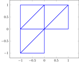
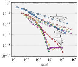
Figure 2: Initial triangulation $\mathcal{T}_{0}$ (left) of the L-shaped domain and convergence history plot (right) of $|E(u)-E_{\ell}(u_{\ell})|$ with $k$ from Figure 1 on uniform (dashed line) and adaptive (solid line) triangulations for the $p$-Laplace benchmark in Subsection 6.2

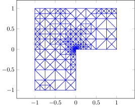
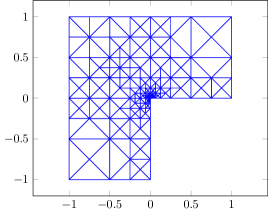
Figure 3: Adaptive triangulations of the L-shaped domain into 492 triangles (1238 dofs) for $k=0$ (left) and 490 triangles (7824 dofs) for $k=3$ (right) for the $p$-Laplace benchmark in Subsection 6.2

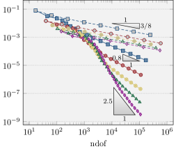
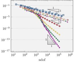
Figure 4: Convergence history plot of $\|\nabla u-\mathcal{G}_{\ell}u_{\ell}\|_{L^{4}(\Omega)}^{2}$ (left) and $\|\sigma-\nabla W(\mathcal{G}_{\ell}u_{\ell})\|_{L^{4/3}(\Omega)}^{2}$ (right) with $k$ from Figure 1 on uniform (dashed line) and adaptive (solid line) triangulations for the $p$-Laplace benchmark in Subsection 6.2

The third numerical benchmark from [15, Section 6] for the $p$-Laplace problem in Subsection 2.4.1 considers $p=4$, the right-hand side

$$f(r,\varphi)\coloneqq 343/2048r^{-11/8}\sin(7\varphi/8),$$

on the L-shaped domain $\Omega\coloneqq(-1,1)^{2}\setminus([0,1)\times(-1,0])$ with the initial triangulation $\mathcal{T}_{0}$ displayed in Figure 2.a, the Dirichlet boundary data $u_{\mathrm{D}}(r,\varphi)\coloneqq r^{7/8}\sin(7\varphi/8)$ $\Gamma_{\mathrm{D}}\coloneqq({0}\times[-1,0])\cup([0,1]\times{0})$, and the Neumann boundary data

$$g(r,\varphi)\coloneqq 343/512r^{-3/8}(-\sin(\varphi/8),\cos(\varphi/8))\cdot\nu$$

in polar coordinates with the outer normal unit vector $\nu$ on $\Gamma_{\mathrm{N}}\coloneqq\partial\Omega\setminus\Gamma_{\mathrm{D}}$. The minimal energy $\min E(\mathcal{A})=-1.4423089582447$ is attained at the unique minimizer

$$u(r,\varphi)\coloneqq r^{7/8}\sin(7\varphi/8).$$

Since $u$ is singular at the origin, reduced convergence rates are expected for uniform mesh-refining. Figure 2.b displays the suboptimal convergence rates $0.75$ for the energy error $|E(u)-E_{\ell}(u_{\ell})|$ and all polynomial degrees $k=0,\dots,4$. The adaptive mesh-refining algorithm refines towards the origin as depicted in Figure 3 and we observed a stronger local refinement for larger polynomial degree $k$. Since $W$ satisfies (2.5)–(2.6), the interest is on the displacement error $\|\nabla u-\mathcal{G}_{\ell}u_{\ell}\|_{L^{4}(\Omega)}$ and the stress error $\|\sigma-\nabla W(\mathcal{G}_{\ell}u_{\ell})\|_{L^{4/3}(\Omega)}$. On uniformly refined meshes, $\|\nabla u-\mathcal{G}_{\ell}u_{\ell}\|_{L^{4}(\Omega)}^{2}$ converges with the suboptimal convergence rate $0.375$ and adaptive computation improves the convergence rate to $0.8$ for $k=0$ and $2.5$ for $k=4$ as depicted in Figure 4.a. Figure 4.b displays the convergence rate $1$ for the stress error $\|\sigma-\nabla W(\mathcal{G}_{\ell}u_{\ell})\|_{L^{4/3}(\Omega)}^{2}$ on uniform triangulations for all $k=0,\dots,4$. This is optimal for $k=0$, but not for $k\geq 1$. The adaptive mesh-refining algorithm recovers the optimal convergence rates $k+1$ for $k\geq 1$.

6.3 The optimal design problem

Consider $W$ from Subsection 2.4.2 for $\mu_{1}=1$, $\mu_{2}=2$, $\xi_{1}=\sqrt{2\lambda\mu_{1}/\mu_{2}}$, and $\xi_{2}=\mu_{2}\xi_{1}/\mu_{1}$ with the fixed parameter $\lambda=0.0145$ on the L-shaped domain $\Omega\coloneqq(-1,1)^{2}\setminus([0,1)\times(-1,0])$ from [4, Figure 1.1]. Let $f\equiv 1$ in $\Omega$ and $u_{\mathrm{D}}\equiv 0$ on $\Gamma_{\mathrm{D}}=\partial\Omega$ with the reference value $\min E(\mathcal{A})=-0.0745512$.

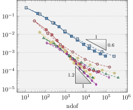
Figure 5: Material distribution of the L-shaped domain (left) and convergence history plot (right) of $\mathrm{RHS}_{\ell}$ in (6.1) with $k$ from Figure 1 on uniform (dashed line) and adaptive (solid line) triangulations for the optimal design problem in Subsection 6.3

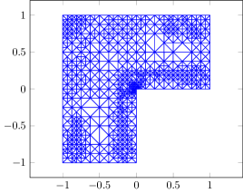
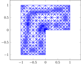
Figure 6: Adaptive triangulation of the L-shaped domain into 1510 triangles (3721 dofs) for $k=0$ (left) and 1351 triangles (21450 dofs) for $k=3$ (right) for the optimal design problem in Subsection 6.3

The material distribution in Figure 5.a consists of two homogenous phases, an interior (red) and a boundary (yellow) layer, and a transition layer, also called microstructure zone with a fine mixture of the two materials [4, 16, 25, 28]. The approximated volume fractions $\Lambda(|\Pi_{\mathcal{T}_{\ell}}^{0}\mathcal{G}_{\ell}u_{\ell}|)$ for a discrete minimizer $u_{\ell}$ with $\Lambda(\xi)=0$ if $0\leq\xi\leq\xi_{1}$, $\Lambda(\xi)=(\xi-\xi_{1})/(\xi_{2}-\xi_{1})$ if $\xi_{1}\leq\xi\leq\xi_{2}$, and $\Lambda(\xi)=1$ if $\xi\geq\xi_{2}$, define the colour map of the fraction plot of Figure 5. Since $W$ satisfies (2.6), Theorem 2.1 implies the convergence of $|E(u)-E_{\ell}(u_{\ell})|$ and $\|\sigma-\nabla W(\mathcal{G}_{\ell}u_{\ell})\|_{L^{2}(\Omega)}$. Since the exact solution is unknown, the numerical experiment computes $\mathrm{RHS}_{\ell}$ in

$$\begin{split}&\|\sigma-\nabla W(\mathcal{G}_{\ell}u_{\ell})\|_{L^{2}(\Omega)}^{2}+|E(u)-E_{\ell}(u_{\ell})|\\ &\qquad\lesssim\mathrm{RHS}_{\ell}\coloneqq E_{\ell}(u_{\ell})-E^{*}(\sigma_{\ell})+\mathrm{osc}(f,\mathcal{T}_{\ell})+\|\mathcal{G}_{\ell}u_{\ell}-\nabla\mathcal{J}_{\ell}u_{\ell}\|_{L^{2}(\Omega)}^{2}\end{split}$$ (6.1)

from [28, Theorem 4.6] with the convex conjugate $W^{*}\in C(\mathbb{M})$ [53, Corollary 12.2.2] and the dual energy

$$E^{*}(\sigma_{\ell})\coloneqq-\int_{\Omega}W^{*}(\sigma_{\ell})\,\mathrm{d}x.$$ (6.2)

Figure 5.b displays the suboptimal convergence rate 0.4 for $\mathrm{RHS}_{\ell}$ on uniform triangulations. The adaptive algorithm refines towards the reentrant corner and the boundaries of the microstructure zone as displayed in Figure 6. This improves the convergence rates up to $1.2$ for $k=4$. Undisplayed computer experiments show significant improvement for the convergence rates of $\mathrm{RHS}_{\ell}$ for examples with small microstructure zones in agreement with the related empirical observations in [25].

6.4 The relaxed two-well benchmark

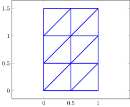
Figure 7: Initial triangulation (left) of the rectangular domain $\Omega$ and convergence history plot (right) of $|E(u)-E_{\ell}(u_{\ell})|$ with $k$ from Figure 1 on uniform (dashed line) and adaptive (solid line) triangulations for the two-well benchmark in Subsection 6.4

Let $\Omega\coloneqq(0,1)\times(0,3/2)$ with pure Dirichlet boundary $\Gamma_{\mathrm{D}}\coloneqq\partial\Omega$. The computational benchmark from [15] considers the two distinct wells $F_{1}=-(3,2)/\sqrt{13}=-F_{2}$ in the definition of $W$ from Subsection 2.4.3 and introduces an additional quadratic term $\|\zeta-v\|_{L^{2}(\Omega)}^{2}$ in the energy

$$E(v)\coloneqq\int_{\Omega}(W(\nabla v)-fv)\,\mathrm{d}x+\|\zeta-v\|_{L^{2}(\Omega)}^{2}/2$$

for all $v\in\mathcal{A}\coloneqq u_{\mathrm{D}}+W^{1,4}_{0}(\Omega)$ with $f(x,y)\coloneqq-3\varrho^{5}/128-\varrho^{3}/3$, $\zeta(x,y)\coloneqq\varrho^{3}/24+\varrho$,

$$u(x,y)\coloneqq u_{\mathrm{D}}(x,y)\coloneqq\begin{cases}f(x,y)&\mbox{if }-1/2\leq\varrho\leq 0,\\ \zeta(x,y)&\mbox{if }0\leq\varrho\leq 1/2\end{cases}$$

at $(x,y)\in\mathbb{R}^{2}$ and $\varrho\coloneqq(3(x-1)+2y)/\sqrt{13}$. Since $E$ is strictly convex in $\mathcal{A}$, the minimal energy $\min E(\mathcal{A})=E(u)=0.1078147674$ is attained at the unique minimizer $u$. The discrete minimizer $u_{\ell}=(u_{\mathcal{T}_{\ell}},u_{\mathcal{F}_{\ell}})$ of the discrete energy

$$E_{\ell}(v_{\ell})\coloneqq\int_{\Omega}(W(\mathcal{G}_{\ell}v_{\ell})-fv_{\mathcal{T}_{\ell}})\,\mathrm{d}x+\|\zeta-v_{\mathcal{T}_{\ell}}\|_{L^{2}(\Omega)}^{2}/2\text{ among }v_{\ell}=(v_{\mathcal{T}_{\ell}},v_{\mathcal{F}_{\ell}})\in\mathcal{A}(\mathcal{T}_{\ell})$$

is unique in the volume component $u_{\mathcal{T}_{\ell}}$ only. The convergence analysis can be extended to the situation at hand with the refinement indicator $\widetilde{\eta}_{\ell}^{(\varepsilon)}(T)\coloneqq\eta_{\ell}^{(\varepsilon)}(T)+|T|\|(1-\Pi_{T}^{k})\zeta\|_{L^{2}(T)}^{2}$ and leads to $\lim_{\ell\to\infty}E_{\ell}(u_{\ell})=E(u)$, $\lim_{\ell\to\infty}\nabla W(\mathcal{G}_{\ell}u_{\ell})=\sigma$ (strongly) in $L^{4/3}(\Omega;\mathbb{R}^{2})$, and $\lim_{\ell\to\infty}u_{\mathcal{T}_{\ell}}=u$ (strongly) in $L^{4}(\Omega)$.

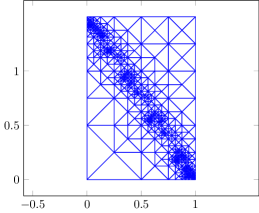
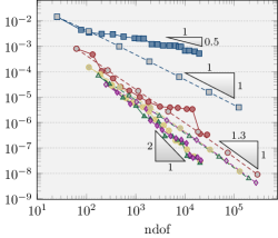
Figure 8: Adaptive triangulation (left) of the rectangular domain $\Omega$ into 1192 triangles (7104 dofs) for $k=1$ and convergence history plot (right) of $\|u-u_{\mathcal{T}_{\ell}}\|_{L^{2}(\Omega)}^{2}$ with $k$ from Figure 1 on uniform (dashed line) and adaptive (solid line) triangulations for the two-well benchmark in Subsection 6.4

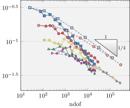
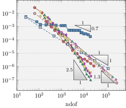
Figure 9: Convergence history plot of $\|\nabla u-\mathcal{G}_{\ell}u_{\ell}\|_{L^{4}(\Omega)}^{2}$ (left) and $\|\sigma-\nabla W(\mathcal{G}_{\ell}u_{\ell})\|_{L^{4/3}(\Omega)}^{2}$ (right) with $k$ from Figure 1 on uniform (dashed line) and adaptive (right) triangulations for the two-well benchmark in Subsection 6.4

The exact solution $u$ is piecewise smooth and the derivative $\nabla u$ jumps across the interface $\Gamma=\mathrm{conv}\{(1,0),(0,3/2)\}$. For an aligned initial triangulation, where $\Gamma$ coincides with the sides of the triangulation, the numerical results from [28] display optimal convergence rates $k+1$ for $|E(u)-E_{\ell}(u_{\ell})|$, $\|\sigma-\sigma_{\ell}\|_{L^{4/3}(\Omega)}^{2}$ $\|u-u_{\mathcal{T}_{\ell}}\|_{L^{2}(\Omega)}^{2}$, and $\|\nabla u-\mathcal{G}_{\ell}u_{\ell}\|_{L^{4}(\Omega)}^{2}$ on uniformly refined meshes. Since a priori information on $u$ is not available in general, this numerical benchmark considers the non-aligned initial triangulation $\mathcal{T}_{0}$ in Figure 7.a, where $\Gamma$ cannot be resolved exactly (even not with adaptively refined triangulations of $\mathcal{T}_{0}$). In this case, [14] predicted

$$\|(1-\Pi_{\mathcal{T}_{\ell}}^{0})u\|_{L^{4}(\Omega)}+\|(1-\Pi_{\mathcal{T}_{\ell}}^{0})\sigma\|_{L^{4/3}(\Omega)}\lesssim H_{\ell},\|(1-\Pi_{\mathcal{T}_{\ell}}^{0})\nabla u\|_{L^{4}(\Omega)}\lesssim H_{\ell}^{1/4}$$

for $H_{\ell}\coloneqq\|h_{\ell}\|_{L^{\infty}(\Omega)}$. These expected (optimal) convergence rates on uniform meshes are indeed observed empirically for the lowest-order HHO scheme. Figure 7.b, Figure 8.b, and Figure 9 displays the convergence rate $1$, $1$, $1/4$, and $1$ for $|E(u)-E_{\ell}(u_{\ell})|$, $\|u-u_{\mathcal{T}_{\ell}}\|_{L^{2}(\Omega)}^{2}$, $\|\nabla u-\mathcal{G}_{\ell}u_{\ell}\|_{L^{4}(\Omega)}^{2}$, and $\|\sigma-\nabla W(\mathcal{G}_{\ell}u_{\ell})\|_{L^{4/3}(\Omega)}^{2}$, respectively. This improves the convergence rate $3/4$ of the stress error from the lowest-order Courant FEM in [14]. The adaptive algorithm generates adaptive meshes with a strong local mesh-refinement near the interface $\Gamma$ and improve the convergence rate of $|E(u)-E_{\ell}(u_{\ell})|$ to $2.2$ in Figure 7.b, of $\|u-u_{\mathcal{T}_{\ell}}\|_{L^{2}(\Omega)}^{2}$ to $2$ in Figure 8.b, and of $\|\sigma-\nabla W(\mathcal{G}_{\ell}u_{\ell})\|_{L^{4/3}(\Omega)}^{2}$ to $2.5$ in Figure 9.b for polynomial degrees $k\geq 2$. For $k=1$, adaptive mesh refinements only leads to marginal improvements. Since optimal convergence rates are obtained for $\|u-u_{\mathcal{T}_{\ell}}\|_{L^{2}(\Omega)}$ and $\|\sigma-\nabla W(\mathcal{G}_{\ell}u_{\ell})\|_{L^{4/3}(\Omega)}$ with $k=0$ on uniform meshes, there is not much gain from adaptive computation.

6.5 Modified Foss-Hrusa-Mizel benchmark

The final example considers a modified Foss-Hrusa-Mizel [43] benchmark in [52], extended to the domain $\Omega\coloneqq(-1,1)\times(0,1)$ with $\Gamma_{1}\coloneqq[-1,0]\times\{0\}$, $\Gamma_{2}\coloneqq[0,1]\times\{0\}$, $\Gamma_{3}\coloneqq\{x=(x_{1},x_{2})\in\partial\Omega:x_{1}=-1\text{ or }x_{1}=1\text{ or }x_{2}=1\}$, and the initial triangulation $\mathcal{T}_{0}$ of Figure 10.a. Define the energy density $W(A)\coloneqq(|A|^{2}-2\det A)^{4}+|A|^{2}/2$ for all $A\in\mathbb{M}\coloneqq\mathbb{R}^{2\times 2}$, the set

$$\mathcal{A}\coloneqq\{v=(v_{1},v_{2})\in W^{1,2}(\Omega;\mathbb{R}^{2}):v_{1}\equiv 0\text{ on }\Gamma_{1},v_{2}\equiv 0\text{ on }\Gamma_{2},v=u_{\mathrm{D}}\text{ on }\Gamma_{3}\}$$

of admissible functions in $W^{1,2}(\Omega;\mathbb{R}^{2})$ with $u_{\mathrm{D}}\coloneqq(\cos(\varphi/2),\sin(\varphi/2))$ in polar coordinates, and the vanishing right-hand side $f\equiv 0$. The minimal energy $E(u)=\min E(\mathcal{A})=0.88137023556$ of

$$E(v)\coloneqq\int_{\Omega}W(\mathrm{D}v)\,\mathrm{d}x\text{ among }v\in\mathcal{A}$$

is attained at $u\coloneqq r^{1/2}(\cos(\varphi/2),\sin(\varphi/2))$ in polar coordinates. The energy density $W\in C^{1}(\mathbb{M})$ is convex and satisfies the lower growth $W(A)\geq|A|^{2}/2$ of order $p=2$, but no upper growth of order $2$.

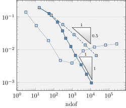
Figure 10: Initial triangulation $\mathcal{T}_{0}$ (left) of $\Omega$ and empirical verification of the Lavrentiev gap (right) for the modified Foss-Hrusa-Mizel benchmark in Subsection 6.5: convergence history plot of $|E(u)-E_{\ell}(u_{\ell})|$ for the Courant FEM (dotted line) and the lowest-order HHO method on uniform (dashed line) and adaptive (solid line) triangulations

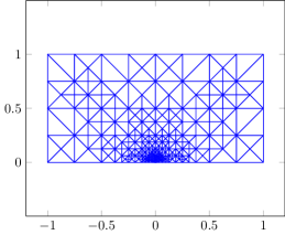
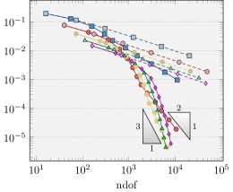
Figure 11: Adaptive triangulation of $\Omega$ (left) into 614 triangles (7336 dofs) for $k=1$ and convergence history plot (right) of $|E(u)-E_{\ell}(u_{\ell})|$ with $k$ from Figure 1 on uniform (dashed line) and adaptive (solid line) triangulations for the modified Foss-Hrusa-Mizel benchmark in Subsection 6.5

The application of the discrete compactness to this model example with free boundary requires the modified refinement indicator

$$\eta_{\ell}^{(\varepsilon)}(T)\coloneqq|T|^{\varepsilon-1}\|\Pi_{T}^{k}((\mathcal{R}_{\ell}u_{\ell})|_{T}-u_{T})\|^{2}_{L^{2}(T)}+|T|^{\varepsilon-1/2}$$

$$\qquad\times\Big{(}\sum_{F\in\mathcal{F}_{\ell}(T)\cap\mathcal{F}_{\ell}(\Gamma_{1})}\|(\mathcal{R}_{\ell}u_{\ell})|_{F}\cdot e_{1}\|_{L^{2}(F)}^{2}+\sum_{F\in\mathcal{F}_{\ell}(T)\cap\mathcal{F}_{\ell}(\Gamma_{2})}\|(\mathcal{R}_{\ell}u_{\ell})|_{F}\cdot e_{2}\|_{L^{2}(F)}^{2}$$

$$\qquad\qquad+\sum_{F\in\mathcal{F}_{\ell}(T)\cap\mathcal{F}_{\ell}(\Gamma_{3})}\|(\mathcal{R}_{\ell}u_{\ell})|_{F}-u_{\mathrm{D}}\|_{L^{2}(F)}^{2}+\sum_{E\in\mathcal{F}_{\ell}(T)\cap\mathcal{F}_{\ell}(\Omega)}\|[\mathcal{R}_{\ell}u_{\ell}]_{F}\|_{L^{2}(F)}^{2}$$

$$\qquad\qquad+\sum_{F\in\mathcal{F}_{\ell}(T)}\|\Pi_{F}((\mathcal{R}_{\ell}u_{\ell})_{T}-u_{F})\|_{L^{2}(F)}^{2}\Big{)}$$

with the $j$-th canonical unit vector $e_{j}\in\mathbb{R}^{2}$. Since the presence of the Lavrentiev gap is equivalent to the failure of conforming FEMs [17, Theorem 2.1], the lowest-order HHO can be utilized to detect the Lavrentiev gap, cf. Subsection 4.3. Figure 10.b provides empirical evidence that there is a Lavrentiev gap: $|E(u)-E_{\ell}(u_{\ell})|$ converges with the suboptimal convergence rate $0.5$ on uniformly refined meshes, but the Courant FEM seems to approximate a wrong energy. The adaptive mesh-refining algorithm refines towards the origin as depicted in Figure 11.a. It is outlined in Subsection 4.3 that a convergence proof of AHHO for minimization problems with the Lavrentiev gap is impossible with the known mathematical methodology for $k\geq 1$. It comes as a welcome surprise that optimal convergence rates $k+1$ are obtained for any polynomial degrees $k$ on adaptively refined meshes in Figure 11.b.

6.6 Conclusions

The numerical results from Section 6 confirm the theoretical findings in Theorem 2.1. In particular, the convergence of the energy $\lim_{\ell\to\infty}\min E_{\ell}(\mathcal{A}(\mathcal{T}_{\ell}))=\min E(\mathcal{A})$ is observed in all examples. The introduced adaptive mesh-refining algorithm of Subsection 2.2 provides efficient approximations of singular solutions and even leads to improved empirical convergence rates. The choice of the parameter $\varepsilon$ only has marginal influence on the convergence rates and convergence is observed for $\varepsilon=0$ in undisplayed computer experiments. Better convergence rates are obtained for larger polynomial degrees $k$. The computer experiments provide empirical evidence that the HHO method can overcome the Lavrentiev gap for any polynomial degree $k$.

Acknowledgement.

This work has been supported by the Deutsche Forschungsgemeinschaft (DFG) in the Priority Program 1748 Reliable simulation techniques in solid mechanics: Development of non-standard discretization methods, mechanical and mathematical analysis under the project CA 151/22.

References

- [1] M. Abbas, A. Ern and N. Pignet “Hybrid high-order methods for finite deformations of hyperelastic materials” In Comput. Mech. 62.4, 2018, pp. 909–928 DOI: 10.1007/s00466-018-1538-0
- [2] Jochen Alberty, Carsten Carstensen and Stefan A. Funken “Remarks around 50 lines of Matlab: short finite element implementation” In Numer. Algorithms 20.2-3, 1999, pp. 117–137 DOI: 10.1023/A:1019155918070
- [3] Anna Kh. Balci, Christoph Ortner and Johannes Storn “Crouzeix-Raviart finite element method for non-autonomous variational problems with Lavrentiev gap” In arXiv:2106. 06837, 2021
- [4] Sören Bartels and Carsten Carstensen “A convergent adaptive finite element method for an optimal design problem” In Numer. Math. 108.3, 2008, pp. 359–385 DOI: 10.1007/s00211-007-0122-x
- [5] Liudmila Belenki, Lars Diening and Christian Kreuzer “Optimality of an adaptive finite element method for the -Laplacian equation” In IMA J. Numer. Anal. 32.2, 2012, pp. 484–510 DOI: 10.1093/imanum/drr016
- [6] Daniele Boffi, Dietmar Gallistl, Francesca Gardini and Lucia Gastaldi “Optimal convergence of adaptive FEM for eigenvalue clusters in mixed form” In Math. Comp. 86.307, 2017, pp. 2213–2237 DOI: 10.1090/mcom/3212
- [7] Andrea Bonito and Ricardo H. Nochetto “Quasi-optimal convergence rate of an adaptive discontinuous Galerkin method” In SIAM J. Numer. Anal. 48.2, 2010, pp. 734–771 DOI: 10.1137/08072838X
- [8] Susanne C. Brenner and Carsten Carstensen “Finite Element Methods” In Encyclopedia of Computational Mechanics Second Edition American Cancer Society, 2017, pp. 1–47 DOI: https://doi.org/10.1002/9781119176817.ecm2003
- [9] Susanne C. Brenner and L. Ridgway Scott “The mathematical theory of finite element methods” 15, Texts in Applied Mathematics Springer, New York, 2008, pp. xviii+397 DOI: 10.1007/978-0-387-75934-0
- [10] Haim Brezis “Functional analysis, Sobolev spaces and partial differential equations”, Universitext Springer, New York, 2011, pp. xiv+599
- [11] Annalisa Buffa and Christoph Ortner “Compact embeddings of broken Sobolev spaces and applications” In IMA J. Numer. Anal. 29.4, 2009, pp. 827–855 DOI: 10.1093/imanum/drn038
- [12] C. Carstensen and G. Dolzmann “Convergence of adaptive finite element methods for a nonconvex double-well minimisation problem” In Math. Comp. 84, 2015, pp. 2111–2135 DOI: 10.1090/S0025-5718-2015-02947-0
- [13] C. Carstensen and G. Dolzmann “Convergence of adaptive finite element methods for a nonconvex double-well minimization problem” In Math. Comp. 84.295, 2015, pp. 2111–2135 DOI: 10.1090/S0025-5718-2015-02947-0
- [14] C. Carstensen and K. Jochimsen “Adaptive finite element methods for microstructures? Numerical experiments for a 2-well benchmark” In Computing 71.2, 2003, pp. 175–204 DOI: 10.1007/s00607-003-0027-1
- [15] C. Carstensen and R. Klose “A posteriori finite element error control for the p-Laplace problem” In SIAM J. Sci. Comput. 25, 2003, pp. 792–814
- [16] C. Carstensen and D. J. Liu “Nonconforming FEMs for an optimal design problem” In SIAM J. Numer. Anal. 53.2, 2015, pp. 874–894 URL: https://doi.org/10.1137/130927103
- [17] C. Carstensen and C. Ortner “Analysis of a class of penalty methods for computing singular minimizers” In Comput. Methods Appl. Math. 10.2, 2010, pp. 137–163 DOI: 10.2478/cmam-2010-0008
- [18] C. Carstensen and S. Puttkammer “How to prove the discrete reliability for nonconforming finite element methods” In J. Comput. Math 38.1, 2020, pp. 142–175 DOI: https://doi.org/10.4208/jcm.1908-m2018-0174
- [19] C. Carstensen and H. Rabus “Axioms of adaptivity with separate marking for data resolution” In SIAM J. Numer. Anal. 55.6, 2017, pp. 2644–2665 DOI: 10.1137/16M1068050
- [20] C. Carstensen, M. Eigel, R. H. W. Hoppe and C. Löbhard “A review of unified a posteriori finite element error control” In Numer. Math. Theory Methods Appl. 5.4, 2012, pp. 509–558 DOI: 10.4208/nmtma.2011.m1032
- [21] C. Carstensen, M. Feischl, M. Page and D. Praetorius “Axioms of adaptivity” In Comput. Math. Appl. 67.6, 2014, pp. 1195–1253 DOI: 10.1016/j.camwa.2013.12.003
- [22] Carsten Carstensen “Convergence of an adaptive FEM for a class of degenerate convex minimization problems” In IMA J. Numer. Anal. 28.3, 2008, pp. 423–439 DOI: 10.1093/imanum/drm034
- [23] Carsten Carstensen, Dietmar Gallistl and Mira Schedensack “Adaptive nonconforming Crouzeix-Raviart FEM for eigenvalue problems” In Math. Comp. 84.293, 2015, pp. 1061–1087 DOI: 10.1090/S0025-5718-2014-02894-9
- [24] Carsten Carstensen and Joscha Gedicke “An adaptive finite element eigenvalue solver of asymptotic quasi-optimal computational complexity” In SIAM J. Numer. Anal. 50.3, 2012, pp. 1029–1057 DOI: 10.1137/090769430
- [25] Carsten Carstensen, David Günther and Hella Rabus “Mixed finite element method for a degenerate convex variational problem from topology optimization” In SIAM J. Numer. Anal. 50.2, 2012, pp. 522–543 DOI: 10.1137/100806837
- [26] Carsten Carstensen and Neela Nataraj “A priori and a posteriori error analysis of the Crouzeix-Raviart and Morley FEM with original and modified right-hand sides” In Comput. Methods Appl. Math. 21.2, 2021, pp. 289–315 DOI: 10.1515/cmam-2021-0029
- [27] Carsten Carstensen and Petr Plecháč “Numerical solution of the scalar double-well problem allowing microstructure” In Math. Comp. 66.219, 1997, pp. 997–1026 URL: https://doi.org/10.1090/S0025-5718-97-00849-1
- [28] Carsten Carstensen and Tien Tran “Unstabilized Hybrid High-order Method for a Class of Degenerate Convex Minimization Problems” In SIAM J. Numer. Anal. 59.3, 2021, pp. 1348–1373 DOI: 10.1137/20M1335625
- [29] J. Manuel Cascon, Christian Kreuzer, Ricardo H. Nochetto and Kunibert G. Siebert “Quasi-optimal convergence rate for an adaptive finite element method” In SIAM J. Numer. Anal. 46.5, 2008, pp. 2524–2550 DOI: 10.1137/07069047X
- [30] Michel Chipot and Charles Collins “Numerical approximations in variational problems with potential wells” In SIAM J. Numer. Anal. 29.4, 1992, pp. 1002–1019 DOI: 10.1137/0729061
- [31] M. Crouzeix and P.-A. Raviart “Conforming and nonconforming finite element methods for solving the stationary Stokes equations. I” In RAIRO Sér. Rouge 7.R-3, 1973, pp. 33–75
- [32] B. Dacorogna “Direct methods in the calculus of variations” 78, Applied Mathematical Sciences Springer, New York, 2008, pp. xii+619
- [33] Xiaoying Dai, Jinchao Xu and Aihui Zhou “Convergence and optimal complexity of adaptive finite element eigenvalue computations” In Numer. Math. 110.3, 2008, pp. 313–355 DOI: 10.1007/s00211-008-0169-3
- [34] Daniele A. Di Pietro and Jérôme Droniou “A hybrid high-order method for Leray-Lions elliptic equations on general meshes” In Math. Comp. 86.307, 2017, pp. 2159–2191 DOI: 10.1090/mcom/3180
- [35] Daniele A. Di Pietro and Alexandre Ern “A hybrid high-order locking-free method for linear elasticity on general meshes” In Comput. Methods Appl. Mech. Engrg. 283, 2015, pp. 1–21 DOI: 10.1016/j.cma.2014.09.009
- [36] Daniele A. Di Pietro and Alexandre Ern “Discrete functional analysis tools for discontinuous Galerkin methods with application to the incompressible Navier-Stokes equations” In Math. Comp. 79.271, 2010, pp. 1303–1330 DOI: 10.1090/S0025-5718-10-02333-1
- [37] Daniele A. Di Pietro, Alexandre Ern and Simon Lemaire “An arbitrary-order and compact-stencil discretization of diffusion on general meshes based on local reconstruction operators” In Comput. Methods Appl. Math. 14.4, 2014, pp. 461–472 DOI: 10.1515/cmam-2014-0018
- [38] Daniele A. Di Pietro and Ruben Specogna “An a posteriori-driven adaptive mixed high-order method with application to electrostatics” In J. Comput. Phys. 326, 2016, pp. 35–55 DOI: 10.1016/j.jcp.2016.08.041
- [39] Daniele Antonio Di Pietro and Jérôme Droniou “The hybrid high-order method for polytopal meshes” Design, analysis, and applications 19, MS&A. Modeling, Simulation and Applications Springer, Cham, [2020] ©2020, pp. 525
- [40] Daniele Antonio Di Pietro and Alexandre Ern “Mathematical aspects of discontinuous Galerkin methods” 69, Mathématiques & Applications (Berlin) [Mathematics & Applications] Springer, Heidelberg, 2012, pp. xviii+384 DOI: 10.1007/978-3-642-22980-0
- [41] Lars Diening and Christian Kreuzer “Linear convergence of an adaptive finite element method for the -Laplacian equation” In SIAM J. Numer. Anal. 46.2, 2008, pp. 614–638 DOI: 10.1137/070681508
- [42] Alexandre Ern and Pietro Zanotti “A quasi-optimal variant of the hybrid high-order method for elliptic partial differential equations with loads” In IMA J. Numer. Anal. 40.4, 2020, pp. 2163–2188 DOI: 10.1093/imanum/drz057
- [43] M. Foss, W. J. Hrusa and V. J. Mizel “The Lavrentiev gap phenomenon in nonlinear elasticity” In Arch. Ration. Mech. Anal. 167.4, 2003, pp. 337–365 DOI: 10.1007/s00205-003-0249-6
- [44] R. Glowinski and A. Marrocco “Sur l’approximation, par éléments finis d’ordre un, et la résolution, par pénalisation-dualité, d’une classe de problèmes de Dirichlet non linéaires” In RAIRO Sér. Rouge Anal. Numér. 9.R-2, 1975, pp. 41–76
- [45] P. C. Hammer, O. J. Marlowe and A. H. Stroud “Numerical integration over simplexes and cones” In Math. Tables Aids Comput. 10, 1956, pp. 130–137
- [46] Robert V. Kohn and Gilbert Strang “Optimal design and relaxation of variational problems. I” In Comm. Pure Appl. Math. 39.1, 1986, pp. 113–137 DOI: 10.1002/cpa.3160390107
- [47] Christian Kreuzer and Emmanuil H. Georgoulis “Corrigendum to “Convergence of adaptive, discontinuous Galerkin methods”” In Math. Comp. 90.328, 2021, pp. 637–640 DOI: 10.1090/mcom/3611
- [48] M. Lavrentieff “Sur quelques problèmes du calcul des variations” In Ann. Mat. Pura Appl. 4.1, 1927, pp. 7–28 DOI: 10.1007/BF02409983
- [49] Pedro Morin, Kunibert G. Siebert and Andreas Veeser “A basic convergence result for conforming adaptive finite elements” In Math. Models Methods Appl. Sci. 18.5, 2008, pp. 707–737 DOI: 10.1142/S0218202508002838
- [50] Ricardo H. Nochetto and Andreas Veeser “Primer of adaptive finite element methods” In Multiscale and adaptivity: modeling, numerics and applications 2040, Lecture Notes in Math. Springer, Heidelberg, 2012, pp. 125–225 DOI: 10.1007/978-3-642-24079-9
- [51] Christoph Ortner “Nonconforming finite-element discretization of convex variational problems” In IMA J. Numer. Anal. 31.3, 2011, pp. 847–864 DOI: 10.1093/imanum/drq004
- [52] Christoph Ortner and Dirk Praetorius “On the convergence of adaptive nonconforming finite element methods for a class of convex variational problems” In SIAM J. Numer. Anal. 49.1, 2011, pp. 346–367 DOI: 10.1137/090781073
- [53] R. Tyrrell Rockafellar “Convex analysis”, Princeton Mathematical Series, No. 28 Princeton University Press, Princeton, N.J., 1970, pp. xviii+451
- [54] Rob Stevenson “Optimality of a standard adaptive finite element method” In Found. Comput. Math. 7.2, 2007, pp. 245–269 DOI: 10.1007/s10208-005-0183-0
- [55] Rob Stevenson “The completion of locally refined simplicial partitions created by bisection” In Math. Comp. 77.261, 2008, pp. 227–241 DOI: 10.1090/S0025-5718-07-01959-X
- [56] Andreas Veeser “Convergent adaptive finite elements for the nonlinear Laplacian” In Numer. Math. 92.4, 2002, pp. 743–770 DOI: 10.1007/s002110100377
- [57] Andreas Veeser and Pietro Zanotti “Quasi-optimal nonconforming methods for symmetric elliptic problems. II—Overconsistency and classical nonconforming elements” In SIAM J. Numer. Anal. 57.1, 2019, pp. 266–292 DOI: 10.1137/17M1151651
- [58] Rüdiger Verfürth “A posteriori error estimation techniques for finite element methods”, Numerical Mathematics and Scientific Computation Oxford University Press, Oxford, 2013, pp. xx+393 DOI: 10.1093/acprof:oso/9780199679423.001.0001